SHARP VIII: J 0924+0219 lens mass distribution and time-delay prediction through adaptive-optics imaging

Abstract

Strongly lensed quasars can provide measurements of the Hubble constant ($H_{0}$) independent of any other methods. One of the key ingredients is exquisite high-resolution imaging data, such as Hubble Space Telescope (HST) imaging and adaptive-optics (AO) imaging from ground-based telescopes, which provide strong constraints on the mass distribution of the lensing galaxy. In this work, we expand on the previous analysis of three time-delay lenses with AO imaging (RXJ 1131$-$1231, HE 0435$-$1223, and PG 1115$+$080), and perform a joint analysis of J 0924+0219 by using AO imaging from the Keck Telescope, obtained as part of the SHARP (Strong lensing at High Angular Resolution Program) AO effort, with HST imaging to constrain the mass distribution of the lensing galaxy. Under the assumption of a flat $\Lambda$CDM model with fixed $\Omega_{\rm m}=0.3$, we show that by marginalizing over two different kinds of mass models (power-law and composite models) and their transformed mass profiles via a mass-sheet transformation, we obtain $\Delta t_{\rm BA}h\hat{\sigma}_{v}^{-2}=6.89\begin{subarray}{c}+0.8\\ -0.7\end{subarray}$ days, $\Delta t_{\rm CA}h\hat{\sigma}_{v}^{-2}=10.7\begin{subarray}{c}+1.6\\ -1.2\end{subarray}$ days, and $\Delta t_{\rm DA}h\hat{\sigma}_{v}^{-2}=7.70\begin{subarray}{c}+1.0\\ -0.9\end{subarray}$ days, where $h=H_{0}/100~{}\rm km\,s^{-1}\,Mpc^{-1}$ is the dimensionless Hubble constant and $\hat{\sigma}_{v}=\sigma^{\rm ob}_{v}/(280~{}\rm km\,s^{-1})$ is the scaled dimensionless velocity dispersion. Future measurements of time delays with 10% uncertainty and velocity dispersion with 5% uncertainty would yield a $H_{0}$ constraint of $\sim 15$% precision.

1 Introduction

Measuring the Hubble constant is one of the most important tasks in modern cosmology especially since not only it sets the age, the size, and the critical density of the Universe but also the recent direct $H_{0}$ measurements from Type Ia supernovae (SNe), calibrated by the traditional Cepheid distance ladder (SH0ES collaboration; Riess et al., 2019), show a $4.4\sigma$ tension with the Planck results under the assumption of $\Lambda$CDM model (e.g., Komatsu et al., 2011; Hinshaw et al., 2013; Planck Collaboration et al., 2018; Anderson et al., 2014; Kazin et al., 2014; Ross et al., 2015). However, a recent measurement of $H_{0}$ from SNe Ia calibrated by the Tip of the Red Giant Branch (TRGB) by the Carnegie-Chicago Hubble Program (CCHP) agrees with both the Planck and SH0ES results within the errors (Freedman et al., 2019, 2020). These results clearly demonstrate that it is crucial to test any single measurement by independent probes.

Strongly lensed quasars provide an independent way to measure the Hubble constant (Refsdal, 1964; Suyu et al., 2017; Treu & Marshall, 2016). With the combination of time delays, high-resolution imaging, the velocity dispersion of the lensing galaxy, and the description of the mass along the line of sight (so-called external mass-sheet transformation; see details in Falco et al., 1985; Gorenstein et al., 1988; Fassnacht et al., 2002; Suyu et al., 2013; Greene et al., 2013; Collett et al., 2013), the TDCOSMO collaboration (Millon et al., 2020) has shown that one can provide robust constraints on both the angular diameter distance to the lens ($D_{\textrm{d}}$; Jee et al., 2015) and the time-delay distance which is a ratio of the angular diameter distances in the system:

$$D_{\Delta\textrm{t}}\equiv\left(1+z_{\rm d}\right)\frac{D_{\textrm{d}}D_{\textrm{s}}}{D_{\textrm{ds}}}\propto H_{0}^{-1},$$ (1)

where $z_{\rm d}$ is the redshift of the lens, $D_{\textrm{s}}$ is the distance to the background source, and $D_{\textrm{ds}}$ is the distance between the lens and the source. These distances are used to determine cosmological parameters, primarily $H_{0}$ (e.g., Suyu et al., 2014; Bonvin et al., 2016; Birrer et al., 2019; Chen et al., 2019; Rusu et al., 2019; Wong et al., 2020; Jee et al., 2019; Taubenberger et al., 2019; Shajib et al., 2020).

A blind analysis done by Wong et al. (2020) with this technique as part of the H0LiCOW program (Suyu et al., 2017), in collaboration with the COSMOGRAIL (e.g., Courbin et al., 2018) and SHARP (Chen et al., 2019, Fassnacht et al. in prep) programs, combined the data from six gravitational lens systems, and inferred $H_{0}=73.3\begin{subarray}{c}+1.7\\ -1.8\end{subarray}~{}\rm km\,s^{-1}\,Mpc^{-1}$, a value that was $3.8\sigma$ away from the Planck results. The above work marginalized over two different kinds of mass profiles for the lensing galaxies in order to better estimate the uncertainties. The first description consists of a NFW dark matter halo (Navarro et al., 1996) plus a constant mass-to-light ratio stellar distribution (the “composite model”). The second description models the three dimensional total mass density distribution, i.e., luminous plus dark matter, of the galaxy as a power law (Barkana, 1998), i.e., $\rho(r)\propto r^{-\gamma}$ (the power-law model). Millon et al. (2020) later combined six lenses from Wong et al. (2020) with one additional lens analyzed by Shajib et al. (2020) in the STRIDES program (Treu et al., 2018), and showed that even if we separate these two descriptions of the mass distribution of the lensing galaxy, the $H_{0}$ measurements are consistent well within 1%. An independent check by Chen et al. (2019) using ground-based high-resolution adaptive optics (AO) imaging data from SHARP with three strongly lensed quasar also shows consistent results with Wong et al. (2020) and is 3.5$\sigma$ away from Planck results.

Given the growing statistical tension between $H_{0}$ measurements, efforts by the TDCOSMO collaboration have gone into studying potential systematic uncertainties (Millon et al., 2020; Gilman et al., 2020). A crucial potential source of uncertainty is the assumptions on the radial density profile. Birrer et al. (2020) introduced a flexible parametrization on the mass model that is maximally degenerate with $H_{0}$ through the mass-sheet trasformation (so-called internal MST; see also Schneider & Sluse, 2013; Xu et al., 2016; Kochanek, 2020, 2021; Chen et al., 2020), as a way to express departures from the standard assumptions in previous work (Blum et al., 2020; Shajib et al., 2021). With this parametrization, the main factor determining the precision of the cosmological inference is the stellar kinematics in the lensing galaxy (see discussion by Treu & Koopmans, 2002; Koopmans et al., 2003; Jee et al., 2016; Birrer et al., 2016; Chen et al., 2020). With the MST parametrization, the uncertainty on $H_{0}$ based on the 7 lens sample of Millon et al. (2020) goes from $\sim$2% to $\sim 8\%$, in a standard $\Lambda$CDM cosmology.

To further constrain the $H_{0}$ value contributed from the MST and anisotropy parameters, Birrer et al. (2020) developed a hierarchical Bayesian framework by including external datasets, assuming they are drawn from the same population. When assuming that the TDCOSMO lenses and the SLACS samples are drawn from the single stellar-orbit anisotropy distribution (Bolton et al., 2004, 2006; Auger et al., 2010), Birrer et al. (2020) inferred $73.3\pm 5.8~{}\rm km\,s^{-1}\,Mpc^{-1}$. Assuming that TDCOSMO and SLACS are also drawn from the same population in terms of both anisotropy and mass density profile, the inference on $H_{0}$ shifted to $67.4\begin{subarray}{c}+4.1\\ -3.2\end{subarray}~{}\rm km\,s^{-1}\,Mpc^{-1}$, which statistically agree with both Planck and SH0ES results. Increasing the number of the time-delay lens systems and using different external datasets are crucial to assess whether the difference between SLACS and TDCOSMO is real or a statistical fluctuation (Birrer & Treu, 2021).

To expand the sample of analyzed AO-observed time-delay lenses (Chen et al., 2019) we study the J 0924+0219 lens system, which has AO imaging and archival HST imaging. In this work, we take into account both the internal and external MST and forecast the time delays. Since the velocity dispersion of the lensing galaxy is not yet measured, we predict the time delay based on the imaging data with the expected precision of the kinematic data. In Section 2, we describe the basic information on J 0924+0219 and describe the data acquisition and analysis; in Section 3, we describe the models we used for fitting the imaging; in Section 4, we make a time-delay prediction based on imaging data under the assumption of a flat $\Lambda$CDM model with fixed $\Omega_{\rm m}=0.3$. The conclusion is in Section 5.

2 J 0924+0219

The J 0924+0219 system (J2000: 09 ${}^{\textrm{h}}$24${}^{\textrm{m}}$55.87, 02°19′24$\aas@@fstack{\prime\prime}$9) is a quadruply-lensed quasar discovered by Inada et al. (2003). The main lensing galaxy is at a redshift of $z_{\rm d}=0.394\pm 0.001$ (Eigenbrod et al., 2006), and the source redshift is $z_{\rm s}=1.524\pm 0.001$ (Inada et al., 2003). The analysis in this paper is based on new Keck AO and archival HST observations of J 0924+0219. We describe the data acquisition and analysis in Section 2.1 and Section 2.2. We show the data from three HST bands and one Keck AO K^′-band in Figure 1.

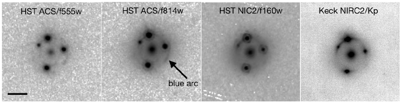
Figure 1: HST and Adaptive optics images of J 0924+0219 gravitational lens systems. The solid horizontal line represents 1″scale. The foreground main lens is located in the center of the lens system. The multiple lensed images and the extended arc around the lensing galaxy are from the background AGN and its host galaxy.

Figure 2: The left figure is the reconstructed AO PSF of J 0924+0219. The right panel is the comparison of the radial average intensity of the reconstructed PSFs from all four AO lenses from previous work (Chen et al., 2019). All the reconstructed PSFs show core structures and extended wings.

2.1 Hubble Space Telescope Imaging

We use optical and near-infrared imaging of the system obtained from the HST archive. The archival data include NICMOS images through the F160W filter (total exposure time: 5311.52 seconds) taken with HST on November 23, 2003 and ACS/WFC images though the F814W filter (total exposure time: 2296 seconds) and F555W filter (total exposure time: 2188 seconds) taken with HST on November 18, 2003 (PID:9744, PI: C. Kochanek). We process the data using AstroDrizzle with standard settings, which removes the geometric distortions, corrects for sky background variations, and flags cosmic-rays. The final drizzled HST images with a scale of 0.05″ per pixel are presented in Figure 1.

2.2 Keck Adaptive Optics Imaging

The AO imaging was obtained at K^′-band with the Near-infrared Camera 2 (NIRC2), as part of the SHARP AO effort (Fassnacht et al., in prep). The target was observed with the narrow camera setup, which provides a roughly 10$\times$10″ field of view and a pixel scale of 10 milliarcsec (mas). There are three exposures of 300 seconds on December 30, 2011, seven exposures of 300 seconds on May 16, 2012, and four exposures of 300 seconds on May 18, 2012. The total exposure time was 4200 seconds. We follow our previous work (Chen et al., 2016, 2019) and use the SHARP python-based pipeline, which performs a flat-field correction, sky subtraction, correction of the optical distortion in the images, and a coadditon of the exposures. For the distortion correction step, the images are resampled to produce final pixel scales of 10 mas pix^-1 for the narrow camera. The narrow camera pixels samples well the AO PSF, which has typical FWHM values of 60–90 mas. To improve the modeling efficiency for the narrow camera data, we perform a 2$\times$2 binning of the images produced by the pipeline to obtain images that have a 20 mas pix^-1 scale. The final HST images are presented in Figure 1.

Figure 3: The comparison of the radial average intensity of the reconstructed AO PSFs and HST PSF of J 0924+0219.

3 J0924+0219 modeling

We describe the PSF models in Section 3.1, lens modeling in Section 3.2, kinematics modeling in Section 3.3, and time-delay prediction model in Section 3.4.

3.1 The PSF of J0924

For the F160W band HST imaging, we use Tinytim (Krist & Hook, 1997) to generate the PSFs with different spectral index, $\hat{\eta}_{v}$, of a power-law from $-0.4$ to $-2.5$ and different focuses from 0 to 10. Given the F160W band HST imaging, we find that the best-fit to the imaging is the PSF with focus equal to 0 and spectral index equal to $-1.3$. We use this Tinytim PSF as the initial guess and then apply the PSF-correction method of Chen et al. (2016) while modeling the F160W HST imaging. For the F814W and F555W bands, that were observed with the ACS with a larger field of view, we use one of the nearby bright stars as the initial guess of the PSF and apply the PSF-correction until the residuals stabilized. For the AO imaging, we follow the criteria described in Section 4.4.3 of Chen et al. (2016) and perform 9 iterative steps to create the final PSF and make sure the size of the PSF for convolution is large enough ($1.18\arcsec\times 1.18\arcsec$) such that the results are stable. The full width half maximum (FWHM) of the AO PSF is $\sim 75$ mas. We show the reconstructed AO PSF in Figure 2 and the comparison of AO and HST PSF in Figure 3.

3.2 Lens imaging modeling

Eigenbrod et al. (2006) first modeled this system with HST imaging and suspected that the second set of bluer arcs in F814W band (see Figure 1) inside and outside the area delimited by the red arcs in F160W band could be either a second source in different redshift or a star forming region in the source galaxy. We examine the possibility of a second source plane existing at a lower redshift than the source ($z=1.52$) due to bluer color and find that the scenario is very unlikely, as the macro model determined by the red arc cannot reproduce a reasonable source for the blue arcs given a possible range of the source redshift from $z=0.5$ to $z<1.52$. In contrast, we do find that a star forming region can be reconstructed at the same source redshift. Faure et al. (2011) modeled the lens with high-resolution H and Ks imaging obtained using the ESO VLT with adaptive optics and the laser guide star system. They identified a luminous object, located $\sim 0.3\arcsec$ to the north of the lens galaxy, but showed that it cannot be responsible for the anomalous flux ratios. Many studies (e.g., Metcalf & Madau, 2001; Bradač et al., 2002; Dalal & Kochanek, 2002; Pooley et al., 2012; Schechter et al., 2014; Glikman et al., 2018; Badole et al., 2020) have shown that the macro model cannot explain the flux ratio, which suggested the presence of microlensing or dark matter substructures. Thus, to avoid possible biases caused by flux ratios, we only use the lensed quasar positions and the extended arc to constrain the mass model, which is also the standard procedure for $H_{0}$ measurements in TDCOSMO collaboration. Gilman et al. (2020) also show that the presence of substructures do not bias $H_{0}$ above the percent level. We use glee, a strong lens modeling code to model three HST bands and one Keck AO band simultaneously (Suyu & Halkola, 2010; Suyu et al., 2012). We describe the models in the following for fitting the high resolution imaging data.

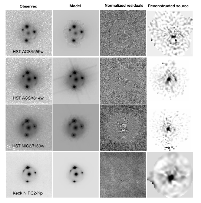
Figure 4: J 0924+0219 HST and AO image reconstruction of the most probable model with a source grid of $53\times 53$ pixels. We use $59\times 59$ pixels of the AO PSF and $29\times 29$ pixels of the HST PSF for convolution of spatially extended images. From left column to right column: observed imaging, model imaging, normalized residuals, and reconstructed source.

We show the imaging, models, normalized residuals, and reconstructed sources in Figure 4. Note that since the source in F555W band has more clumpy star forming region, the reconstructed source is less regular with small-scale structures and more noise. In addition, the noise-overfitting problem is due to the fact that the outer region of the source plane is under-regularized, but this effect will not underestimate the uncertainty because the uncertainty will be dominated by the time-delay and velocity dispersion measurements. Besides, we model the imaging with different source resolutions and marginalize over them to control the systematics.

Table 1: Lens model parameters for power-law model

Description	Parameter	Marginalized
		Constraints
Lens mass distribution
Centroid of G in $\theta_{1}$ (arcsec)	$\theta_{1}$$\clubsuit$	$3.01^{+0.08}_{-0.05}$
Centroid of G in $\theta_{2}$ (arcsec)	$\theta_{2}$	$3.02^{+0.03}_{-0.04}$
Axis ratio of G	$q$	$0.61\pm 0.01$
Position angle of G	$\theta$$\spadesuit$	$-0.04\pm 0.01$
Einstein radius of G (arcsec)	$\theta_{\rm E}$	$0.940^{+0.004}_{-0.003}$
Radial slope of G	$\gamma$	$2.270^{+0.007}_{-0.003}$
External shear strength	$\gamma^{\prime}$	$0.017^{+0.001}_{-0.003}$
External shear angle	$\theta_{\gamma^{\prime}}$	$4.24^{+0.01}_{-0.03}$

• Note: The mass model parameters of power-law model. The source pixel parameters are marginalized. The confidence interval represents 1 $\sigma$ uncertainty. Position angle is counter clockwise from +x in radians.

Figure 5: Marginalized mass-model parameter distributions from the J 0924+0219 power-law lens model results. The description of the parameters are: $q$ is axis ratio of power-law mass profile, $\theta$ is the position angle of power-law mass profile, $\theta_{\rm E}$ is the Einstein radius, $\gamma$ is the slope, $\gamma^{\prime}$ is the strength of the external shear, and $\theta_{\gamma^{\prime}}$ is the orientation of the shear strength. The contours represent the $68.3\%$ and $95.4\%$ quantiles. Position angle is counter clockwise from +x in radians.

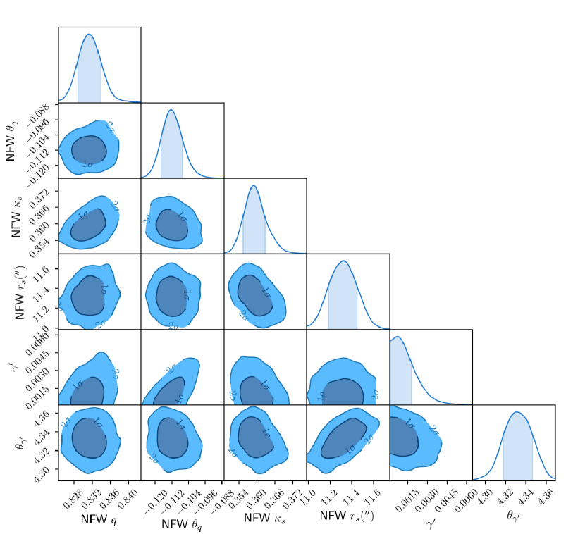
Figure 6: Marginalized parameter distributions from the J 0924+0219 composite lens model results. NFW $q$ is axis ratio of NFW profile, NFW $\theta_{q}$ is the position angle of NFW, NFW $r_{\rm s}$ is the scale radis of NFW profile, $\gamma^{\prime}$ is the strength of the external shear, $\theta_{\gamma^{\prime}}$ is the orientation of the shear strength. The contours represent the $68.3\%$ and $95.4\%$ quantiles. Position angle is counter clockwise from +x in radians.

• Power-law mass model+shear+S$\acute{\text{e}}$rsic light model: we first choose the softened power-law elliptical mass distributions (SPEMD; Barkana, 1998) density profile with the softening length close to zero – the main parameters include radial slope ($\gamma$), Einstein radius ($\theta_{\rm E}$), Position angle ($\theta_{q}$) and the axis ratio of the elliptical isodensity contour ($q$) – to simultaneously model the extended arcs seen in the three HST bands and one AO band, and reconstruct the source structure on a pixelated grid (Suyu et al., 2006). The power-law model is motivated by many studies which have shown that a power-law model provides a good description of the lensing galaxies and dynamical studies for galaxy-galaxy lensing (e.g., Koopmans et al., 2006; Koopmans et al., 2009; Suyu et al., 2009; Auger et al., 2010; Barnabè et al., 2011; Sonnenfeld et al., 2013; Cappellari et al., 2015; Shajib et al., 2021). In the modeling, we found that two concentric S$\acute{\text{e}}$rsic profiles are sufficient to describe the lensing light distribution of the HST F555W and HST F160W bands, while three concentric S$\acute{\text{e}}$rsic profiles are needed for the HST F814W band and Keck AO band. Except for the parameters that describe the lens light center ($\theta_{1,\rm Light}$ and $\theta_{2,\rm Light}$), which are linked together for the light profiles, the light parameters (position angles, ellipticities, and S$\acute{\text{e}}$rsic index) are free. We list all parameters in Table 1 and Table 2, and show the important marginalised mass model parameters in Figure 5.

• Composite mass model+shear+chameleon light profile: we follow Chen et al. (2019) and test a composite (baryonic + dark matter) model. For the dark matter component we adopt the standard NFW profile (Navarro et al., 1996) with the following parameters: halo normalization (NFW $\kappa_{\rm s}$), halo scale radius (NFW $r_{\rm s}$), halo minor-to-major axis ratio (NFW $q$), and associated position angle (NFW $\theta_{q}$). This is motivated by Dutton & Treu (2014), who find that non-contracted NFW profiles are a good representation for the dark matter halos of massive elliptical galaxies (See also Shajib et al., 2021). The baryonic component is modeled by multiplying the lens surface brightness distribution by a constant M/L ratio parameter. For computational efficiency, we model the surface brightness with chameleon profile. The chameleon profile is the difference of two isothermal profiles and is a good approximation to a S$\acute{\text{e}}$rsic profile over the range of interest (see details in Dutton et al., 2011). We link the baryonic matter to the chameleon light profiles of the F160W bands because it probes the rest-frame near-infrared and thus should be the best tracer of stellar mass (See also Chen et al., 2019; Wong et al., 2017). Since the degeneracy between the wings of the AO PSF and lens light could bias the inferred baryonic component, we do not use AO lens light to infer the baryonic distribution (Chen et al., 2019). However, when combining with HST imaging, the well-known HST PSF can provide the information of baryonic distribution (Chen et al., 2019). Future AO imaging with AO PSF reconstructed from telemetry data can break the degeneracy and directly infer the baryonic matter without the need of HST imaging (Chen et al., 2021). We set a Gaussian prior of $r_{s}=15.0\pm 2.0\arcsec$ based on the results of Gavazzi et al. (2007) for lenses in the SLACS sample, which encompasses the redshift of J 0924+0219. We list all parameters in Table 3 and Table 4, and show the important marginalised parameters in Figure 6.

Table 2: Lens light model parameters for power-law model

Lens light as S$\acute{\text{e}}$rsic profiles
Description	Parameter	F555W	F814W	F160W	Keck AO
Centroid of S in $\theta_{1}$ (arcsec)	$\theta_{1,\rm Light}$	$3.0092\pm 0.0002$	$3.0092\pm 0.0002$	$3.0092\pm 0.0002$	$3.0092\pm 0.0002$
Centroid of S in $\theta_{2}$ (arcsec)	$\theta_{2,\rm Light}$	$2.9935\pm 0.0002$	$2.9935\pm 0.0002$	$2.9935\pm 0.0002$	$2.9935\pm 0.0002$
Axis ratio of S1	$q_{\rm S1}$	$0.88^{+0.03}_{-0.04}$	$0.67^{+0.02}_{-0.03}$	$0.89^{+0.02}_{-0.01}$	$0.76\pm 0.03$
Position angle of S1	$\theta_{\rm S1}$	$5.2\pm 0.4$	$6.55^{+0.02}_{-0.06}$	$3.8\pm 0.1$	$-9.12^{+0.07}_{-0.08}$
Amplitude of S1	$I_{\rm s,S1}$$\dagger$	$0.2\pm 0.2$	$0.071^{+0.004}_{-0.01}$	$0.669^{+0.005}_{-0.007}$	$0.41\pm 0.02$
Effective radius of S1 (arcsec)	$R_{\rm eff,S1}$	$0.105\pm 0.005$	$0.95\pm 0.03$	$0.112\pm 0.001$	$0.96\pm 0.03$
Index of S1	$n_{\text{S1}}$	$0.6\pm 0.1$	$0.9\pm 0.1$	$1.25\pm 0.02$	$0.366^{+0.005}_{-0.007}$
Axis ratio of S2	$q_{\rm S2}$	$0.93\pm 0.05$	$0.89^{+0.04}_{-0.08}$	$0.76\pm 0.05$	$0.82^{+0.05}_{-0.06}$
Position angle of S2	$\theta_{\rm S2}$	$0.8\pm 0.1$	$6.7\pm 0.2$	$0.55\pm 0.07$	$-1.7\pm 0.1$
Amplitude of S2	$I_{\rm s,S2}$$\dagger$	$0.00632^{+0.00008}_{-0.0004}$	$2.1\pm 0.1$	$0.023^{+0.002}_{-0.001}$	$6.3^{+1.5}_{-2.2}$
Effective radius of S2 (arcsec)	$R_{\rm eff,S2}$	$1.3\pm 0.1$	$0.104^{+0.007}_{-0.004}$	$0.79^{+0.04}_{-0.07}$	$0.145\pm 0.01$
Index of S2	$n_{\text{S2}}$	$3.2^{+0.4}_{-0.6}$	$1.1^{+0.1}_{-0.1}$	$0.368\pm 0.003$	$0.9\pm 0.2$
Axis ratio of S3	$q_{\rm S3}$	…	$0.52^{+0.08}_{-0.04}$	…	$0.7\pm 0.1$
Position angle of S3	$\theta_{\rm S3}$	…	$7.82^{+0.03}_{-0.04}$	…	$-2.9\pm 0.2$
Amplitude of S3	$I_{\rm s,S3}$$\dagger$	…	$0.29\pm 0.05$	…	$0.29\pm 0.05$
Effective radius of S3 (arcsec)	$R_{\rm eff,S3}$	…	$0.27\pm 0.01$	…	$0.28\pm 0.01$
Index of S3	$n_{\text{S3}}$	…	$0.6^{+0.2}_{-0.1}$	…	$0.5^{+0.2}_{-0.1}$

• Note: The lens lights of all 4 bands share the common centroid. The source pixel parameters are marginalized and are thus not listed. The confidence interval represents 1 $\sigma$ uncertainty. Position angle is counter clockwise from +x in radians.

Table 3: Lens mass model parameters for composite model. The Baryonic component are described by two chameleon profiles that mimic the S$\acute{\text{e}}$rsic profiles. Each chameleon profile is composed of two cored isothermal profiles. We label the two chameleon profiles as B1 and B2.

Description	Parameter	Marginalized
		or Optimized
		Constraints
Lens mass distribution
Mass to light ratio	M/L	$12.1\pm 0.2$
Centroid of B1 in $\theta_{1}$ (arcsec)	$\theta_{1,\rm B1}$$\clubsuit$	$3.0096\pm 0.0002$
Centroid of B1 in $\theta_{2}$ (arcsec)	$\theta_{2,\rm B1}$	$2.9906\pm 0.0002$
Axis ratio of B1	$q_{\rm B1}$	$0.811^{+0.007}_{-0.008}$
Position angle of B1	$\phi_{\rm B1}$$\spadesuit$	$-33.05\pm 0.02$
Amplitude of B1	$I_{\rm s,B1}$$\dagger$	$2.72\pm 0.01$
core radius 1 of B1	$r_{\rm c,1,B1}$	$0.105\pm 0.002$
core radius 2 of B1	$r_{\rm c,2,B2}$	$0.182\pm 0.001$
Axis ratio of B2	$q_{\rm B2}$	$0.46\pm 0.01$
Position angle of B2	$\phi_{\rm B2}$$\spadesuit$	$-34.33\pm 0.02$
Amplitude of B2	$I_{\rm s,B2}$$\dagger$	$4.89\pm 0.01$
core radius 1 of B2	$r_{\rm c,1,B2}$	$0.020\pm 0.001$
core radius 2 of B2	$r_{\rm c,2,B2}$	$0.06\pm 0.02$
Centroid of NFW in $\theta_{1}$ (arcsec)	NFW $\theta_{1}$$\clubsuit$	$2.90\pm 0.03$
Centroid of NFW in $\theta_{2}$ (arcsec)	NFW $\theta_{2}$	$3.093^{+0.005}_{-0.05}$
Axis ratio of NFW	NFW $q$	$0.83\pm 0.02$
Position angle of NFW	NFW $\theta_{q}$$\spadesuit$	$-0.11^{+0.05}_{-0.04}$
Amplitude of NFW	NFW $\kappa_{\rm s}$$\dagger$	$0.359\pm 0.003$
core radius of NFW	NFW $r_{\rm s}(\arcsec)$	$11.3\pm 0.1$
External shear strength	$\gamma^{\prime}$	$0.001\pm 0.001$
External shear angle	$\theta_{\gamma^{\prime}}$	$4.3\pm 0.1$

• Note: The mass model parameters of composite model. The source pixel parameters are marginalized and are thus not listed. The confidence interval represents 1 $\sigma$ uncertainty. Position angle is counter clockwise from +x in radians.

Table 4: Lens model parameters for composite model.

Description	Parameter	F555W	F814W	F160W	Keck AO
Lens light as S$\acute{\text{e}}$rsic profiles
Axis ratio of S1	$q_{\rm S1}$	$0.92\pm 0.03$	$0.67^{+0.02}_{-0.03}$	…	$0.75\pm 0.03$
Position angle of S1	$\phi_{\rm S1}$	$4.9\pm 0.2$	$6.55^{+0.02}_{-0.06}$	…	$-9.11^{+0.07}_{-0.08}$
Amplitude of S1	$I_{\rm s,S1}$$\dagger$	$0.158\pm 0.007$	$0.072^{+0.004}_{-0.01}$	…	$0.40\pm 0.02$
Effective radius of S1 (arcsec)	$R_{\rm eff,S1}$	$0.175\pm 0.005$	$0.96^{+0.03}_{-0.02}$	…	$0.96^{+0.03}_{-0.02}$
Index of S1	$n_{\text{S}\acute{\text{e}}\text{rsic},\rm S1}$	$1.69\pm 0.09$	$0.86^{+0.1}_{-0.07}$	…	$0.365^{+0.006}_{-0.007}$
Axis ratio of S2	$q_{\rm S2}$	$0.72\pm 0.04$	$0.89^{+0.05}_{-0.08}$	…	$0.83^{+0.05}_{-0.06}$
Position angle of S2	$\phi_{\rm S2}$	$0.28\pm 0.07$	$6.6\pm 0.2$	…	$-1.7\pm 0.1$
Amplitude of S2	$I_{\rm s,S2}$$\dagger$	$0.0046\pm 0.0004$	$2.1\pm 0.1$	…	$6.3^{+1.5}_{-2.2}$
Effective radius of S2 (arcsec)	$R_{\rm eff,S2}$	$2.11^{+0.08}_{-0.07}$	$0.100^{+0.007}_{-0.004}$	…	$0.15\pm 0.01$
Index of S2	$n_{\text{S}\acute{\text{e}}\text{rsic},\rm S2}$	$1.1\pm 0.1$	$1.06^{+0.07}_{-0.1}$	…	$0.9^{+0.3}_{-0.2}$
Axis ratio of S3	$q_{\rm S3}$	…	$0.52^{+0.08}_{-0.04}$	…	$0.7\pm 0.1$
Position angle of S3	$\phi_{\rm S3}$	…	$7.82^{+0.03}_{-0.04}$	…	$-2.8\pm 0.2$
Amplitude of S3	$I_{\rm s,S3}$$\dagger$	…	$0.29\pm 0.04$	…	$0.28\pm 0.04$
Effective radius of S3 (arcsec)	$R_{\rm eff,S3}$	…	$0.27\pm 0.01$	…	$0.27\pm 0.02$
Index of S3	$n_{\text{S}\acute{\text{e}}\text{rsic},\rm S3}$	…	$0.6\pm 0.2$	…	$0.6^{+0.3}_{-0.2}$

• Note: The lens lights of all 4 bands share the common centroid. The source pixel parameters are marginalized and are thus not listed. S1, S2 and S3 represents three different Sérsic profiles. The confidence interval represents 1 $\sigma$ uncertainty. Position angle is counter clockwise from +x in radians. The lens light parameters for the F160W band are based on chameleon profiles and are used to describe the baryonic lens mass distribution through a constant M/L ratio. These chameleon parameter values for F160W are listed in Table 3.

3.3 Kinematic modeling

To predict the time delays under the presence of the MST, velocity dispersion information is required to constrain the normalization of the 3D de-projected mass model. We follow Sonnenfeld et al. (2012) and calculate the three-dimensional radial velocity dispersion by numerically integrating the solutions of the spherical Jeans equation (Binney & Tremaine, 1987)

$$\frac{1}{\rho_{\ast}}\frac{d(\rho_{\ast}\sigma_{\textrm{r}}^{2})}{dr}+2\frac{\beta_{\textrm{ani}}\sigma_{\textrm{r}}^{2}}{r}=-\frac{GM(r)}{r^{2}},$$ (2)

where $M(r)$ follows either the power-law mass or composite model. For the stellar component, we assume a Hernquist profile (Hernquist, 1990),

$$\rho_{\ast}=\frac{I_{0}a}{2\pi r(r+a)^{3}},$$ (3)

where $I_{0}$ is the normalization term and the scale radius can be related to the effective radius by $a=0.551r_{\textrm{eff}}$. To compare with the data, the seeing-convolved luminosity-weighted line-of-sight velocity dispersion can be expressed as

$$(\sigma^{\textrm{P}}_{v})^{2}=\frac{\int_{\mathcal{A}}[I(R)\sigma_{s}^{2}\ast\mathcal{P}]d\mathcal{A}}{\int_{\mathcal{A}}[I(R)\ast\mathcal{P}]d\mathcal{A}},$$ (4)

where $R$ is the projected radius, $I(R)$ is the light distribution, $\mathcal{P}$ is the PSF convolution kernel (Mamon & Łokas, 2005), and $\mathcal{A}$ is the aperture. The streaming motions (e.g. rotation) are assumed to be zero. The luminosity-weighted line-of-sight velocity dispersion is given by

$$I(R)\sigma_{s}^{2}=2\int^{\infty}_{R}(1-\beta_{\textrm{ani}}\frac{R^{2}}{r^{2}})\frac{\rho_{\ast}\sigma^{2}_{\textrm{r}}rdr}{\sqrt{r^{2}-R^{2}}}.$$ (5)

The predicted velocity dispersion can be simplified and well-approximated (Birrer et al., 2016, 2020; Chen et al., 2020) as

$$(\sigma_{v}^{\textrm{p}})^{2}=(1-\kappa_{\textrm{ext}})\lambda_{\textrm{int}}\left(\frac{D_{\textrm{s}}}{D_{\textrm{ds}}}\right)c^{2}J(\eta_{\textrm{lens}},\eta_{\textrm{light}},\beta_{\textrm{ani}}),$$ (6)

where $J$ contains the angular-dependent information including the parameters describing the 3D deprojected mass distribution, $\eta_{\textrm{lens}}$, the surface-brightness distribution in the lensing galaxy, $\eta_{\textrm{light}}$, and the stellar orbital anisotropy distribution, $\beta_{\textrm{ani}}$. $\kappa_{\textrm{ext}}$ and $\lambda_{\textrm{int}}$ represents the external MST and internal MST, respectively.

We assume the anisotropy component has the form of an anisotropy radius, $r_{\textrm{ani}}$, in the Osipkov-Merritt (OM) formulation (Osipkov, 1979; Merritt, 1985),

$$\beta_{\textrm{ani}}=\frac{r^{2}}{r^{2}_{\textrm{ani}}+r^{2}},$$ (7)

where $r_{\textrm{ani}}=0$ is pure radial orbits and $r_{\textrm{ani}}\rightarrow\infty$ is isotropic with equal radial and tangential velocity dispersions. In our models, we use a scaled version of the anisotropy parameter, $a_{\textrm{ani}}\equiv r_{\textrm{ani}}/r_{\textrm{eff}}$, where $r_{\textrm{eff}}=D_{\textrm{d}}\theta_{\textrm{eff}}$, and $\theta_{\textrm{eff}}$ is the effective radius in angular units. Note that since the LOS velocity dispersion has a degeneracy with the anisotropy parameters (Dejonghe, 1987), we follow Chen et al. (2019) and marginalize the sample of $a_{\textrm{ani}}$ over a uniform distribution $[0.5,5]$.

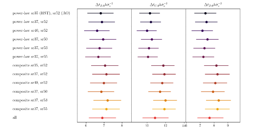
Figure 7: The predicted time delays from the power-law and composite models with different number of reconstructed source pixels for the HST imaging and AO imaging. "sr35 (HST)" represents that we use source grid with 35x35 to reconstructed the backgound source of the HST imaging. All three bands of the HST imaging share the same number of reconstructed sources.

3.4 Time-delay prediction model

The predicted time delay can be expressed as,

$$\Delta t=(1-\kappa_{\textrm{ext}})\lambda_{\textrm{int}}\frac{D_{\Delta\textrm{t}}}{c}\Delta\phi(\theta,\beta),$$ (8)

where $c$ is the speed of light and $\theta$, $\beta$, and $\phi(\theta)$ are the image coordinates, the source coordinates, and the Fermat potential (Blandford & Narayan, 1986) without the presence of internal or external MST respectively. In the case of single aperture velocity dispersion, we can replace the MST terms ($\lambda_{\textrm{int}}$ and $\kappa_{\textrm{ext}}$) with Equation (6) and the predicted time delays will directly relate to the velocity dispersion via

$$\Delta t=(1+z_{\rm d})\frac{D_{\textrm{d}}}{c}\frac{\Delta\phi(\theta,\beta)}{J(\eta_{\textrm{lens}},\eta_{\textrm{light}},a_{\textrm{ani}})}\frac{\sigma_{v}^{2}}{c^{2}}.$$ (9)

The MST-related terms (i.e., $\kappa_{\textrm{ext}}$ and $\lambda_{\textrm{int}}$) canceled out in Equation (9). Thus, the uncertainty of the predicted time delays do not depend on the uncertainty of the mass along the line of sight or transformed mass profile via MST, and only rely on the precision of the velocity dispersion measurement, the redshift of the lens, and the angular diameter distance to the lens (See also similar discussion in Koopmans, 2006). In other words, once the time delay and velocity dispersion are measured, the value of $D_{\textrm{d}}$ can be determined (Chen et al., 2020). When further including environmental information (which provide an estimation of $\kappa_{\textrm{ext}}$) and $D_{\textrm{s}}/D_{\textrm{ds}}$ information which comes from either external datasets or assumption of a cosmological model, one can further determine $\lambda_{\textrm{int}}$ (Birrer et al., 2020; Chen et al., 2020) and use it to further constrain $H_{0}$ with $D_{\Delta\textrm{t}}$ from the population point of view (Birrer et al., 2020). Note that Birrer et al. (2020) use both $D_{\textrm{d}}$ and $D_{\Delta\textrm{t}}$ information to constrain $H_{0}$.

4 Predicted time delays in $\Lambda$CDM cosmology

Due to the lack of velocity dispersion measurement, we express the observed velocity dispersion as $\sigma^{\rm ob}_{v}=\hat{\sigma}_{v}\times 280~{}\rm km\,s^{-1}$, which is created by assuming a flat $\Lambda$CDM with fixed $\Omega_{\rm m}=0.3$, $H_{0}=70~{}\rm km\,s^{-1}\,Mpc^{-1}$, and $\lambda_{\textrm{int}}=1$ (i.e., no internal mass-sheet transformation) in the power-law model (Chen et al., 2020). We fold in an expected $5\%$ uncertainty of the velocity dispersion measurement and present time delay predictions under the assumption of the $\Lambda$CDM model with fixed $\Omega_{\rm m}=0.3$. For the velocity dispersion calculation, we assume the seeing is $1.0\arcsec$ and the aperture size is $1\arcsec\times 1\arcsec$. We show the predicted time delays in Figure 7 with various source resolutions. When we marginalized over different source resolutions of the power-law model, the power-law model predicts $\Delta t_{\rm BA}h\hat{\sigma}_{v}^{-2}=6.75\begin{subarray}{c}+0.78\\ -0.68\end{subarray}$ days, $\Delta t_{\rm CA}h\hat{\sigma}_{v}^{-2}=10.2\begin{subarray}{c}+1.2\\ -1.0\end{subarray}$ days, and $\Delta t_{\rm DA}h\hat{\sigma}_{v}^{-2}=7.31\begin{subarray}{c}+0.86\\ -0.74\end{subarray}$ days. When we marginalized over different source resolutions of the composite model, the composite model predicts $\Delta t_{\rm BA}h\hat{\sigma}_{v}^{-2}=6.99\begin{subarray}{c}+0.81\\ -0.71\end{subarray}$ days, $\Delta t_{\rm CA}h\hat{\sigma}_{v}^{-2}=11.6\begin{subarray}{c}+1.4\\ -1.2\end{subarray}$ days, and $\Delta t_{\rm DA}h\hat{\sigma}_{v}^{-2}=8.10\begin{subarray}{c}+0.96\\ -0.82\end{subarray}$ days. When we marginalized power-law and composite model, we obtain $\Delta t_{\rm BA}h\hat{\sigma}_{v}^{-2}=6.89\begin{subarray}{c}+0.78\\ -0.74\end{subarray}$ days, $\Delta t_{\rm CA}h\hat{\sigma}_{v}^{-2}=10.7\begin{subarray}{c}+1.6\\ -1.2\end{subarray}$ days, and $\Delta t_{\rm DA}h\hat{\sigma}_{v}^{-2}=7.70\begin{subarray}{c}+0.97\\ -0.91\end{subarray}$ days. Given the expected short time delay of this system, it will be challenging to measure the time delays within $10\%$ uncertainty.

5 Conclusions

In this work, we use the high resolution Keck AO imaging data, collected by the SHARP team, and deep HST WFC3 images through the F160W filter, HST ACS/WFC images though F555W filter and F814W filter to simultaneously constrain the mass distribution of J 0924+0219 lens system. When assuming a $\Lambda$CDM model with fixed $\Omega_{\rm m}=0.3$, we find that the power-law model predicts $\Delta t_{\rm BA}h\hat{\sigma}_{v}^{-2}=6.75\begin{subarray}{c}+0.78\\ -0.68\end{subarray}$ days, $\Delta t_{\rm CA}h\hat{\sigma}_{v}^{-2}=10.2\begin{subarray}{c}+1.2\\ -1.0\end{subarray}$ days, and $\Delta t_{\rm DA}h\hat{\sigma}_{v}^{-2}=7.31\begin{subarray}{c}+0.86\\ -0.74\end{subarray}$ days; the composite model (i.e., a NFW dark matter halo (Navarro et al., 1996) plus a constant mass-to-light ratio stellar distribution) predicts $\Delta t_{\rm BA}h\hat{\sigma}_{v}^{-2}=6.99\begin{subarray}{c}+0.81\\ -0.71\end{subarray}$ days, $\Delta t_{\rm CA}h\hat{\sigma}_{v}^{-2}=11.6\begin{subarray}{c}+1.4\\ -1.2\end{subarray}$ days, and $\Delta t_{\rm DA}h\hat{\sigma}_{v}^{-2}=8.10\begin{subarray}{c}+0.96\\ -0.82\end{subarray}$ days. When we marginalized over the power-law and composite model, we obtain $\Delta t_{\rm BA}h\hat{\sigma}_{v}^{-2}=6.89\begin{subarray}{c}+0.78\\ -0.74\end{subarray}$ days, $\Delta t_{\rm CA}h\hat{\sigma}_{v}^{-2}=10.7\begin{subarray}{c}+1.6\\ -1.2\end{subarray}$ days, and $\Delta t_{\rm DA}h\hat{\sigma}_{v}^{-2}=7.70\begin{subarray}{c}+0.97\\ -0.91\end{subarray}$ days. Future measurements of time delays with 10% uncertainty and velocity dispersion with 5% uncertainty would yield a $H_{0}$ constraint of $\sim 15$% precision.

It is important to note that our analysis is truly blind since the time delays and velocity dispersion are not yet measured. Once the velocity dispersion measurement and time delays are measured, the derived posteriors can be used to constrain the $H_{0}$. As part of the TDCOSMO effort, we are getting everything for this lens to have a high-quality $H_{0}$ measurement under the assumptions of standard NFW profile and fixed M/L ratio. These assumptions are in general supported by Shajib et al. (2021) and are currently the standard in the TDCOSMO collaboration. Future work with including varying mass-to-light (M/L) ratio, allowing contracted/expanded NFW profile, and adapting axisymmetric Jeans equations are worth examining the systematics when spatially-resolved kinematics data are obtained.

References

- Anderson et al. (2014) Anderson L., et al., 2014, MNRAS, 441, 24
- Auger et al. (2010) Auger M. W., Treu T., Bolton A. S., Gavazzi R., Koopmans L. V. E., Marshall P. J., Moustakas L. A., Burles S., 2010, ApJ, 724, 511
- Badole et al. (2020) Badole S., Jackson N., Hartley P., Sluse D., Stacey H., Vives-Arias H., 2020, MNRAS, 496, 138
- Barkana (1998) Barkana R., 1998, ApJ, 502, 531
- Barnabè et al. (2011) Barnabè M., Czoske O., Koopmans L. V. E., Treu T., Bolton A. S., 2011, MNRAS, 415, 2215
- Binney & Tremaine (1987) Binney J., Tremaine S., 1987, Galactic dynamics. Princeton, NJ, Princeton University Press, 1987, 747 p.
- Birrer & Treu (2021) Birrer S., Treu T., 2021, A&A, 649, A61
- Birrer et al. (2016) Birrer S., Amara A., Refregier A., 2016, J. Cosmology Astropart. Phys., 8, 020
- Birrer et al. (2019) Birrer S., et al., 2019, MNRAS, 484, 4726
- Birrer et al. (2020) Birrer S., et al., 2020, arXiv e-prints, p. arXiv:2007.02941
- Blandford & Narayan (1986) Blandford R., Narayan R., 1986, ApJ, 310, 568
- Blum et al. (2020) Blum K., Castorina E., Simonović M., 2020, ApJ, 892, L27
- Bolton et al. (2004) Bolton A. S., Burles S., Schlegel D. J., Eisenstein D. J., Brinkmann J., 2004, AJ, 127, 1860
- Bolton et al. (2006) Bolton A. S., Burles S., Koopmans L. V. E., Treu T., Moustakas L. A., 2006, ApJ, 638, 703
- Bonvin et al. (2016) Bonvin V., Tewes M., Courbin F., Kuntzer T., Sluse D., Meylan G., 2016, A&A, 585, A88
- Bradač et al. (2002) Bradač M., Schneider P., Steinmetz M., Lombardi M., King L. J., Porcas R., 2002, A&A, 388, 373
- Cappellari et al. (2015) Cappellari M., et al., 2015, ApJ, 804, L21
- Chen et al. (2016) Chen G. C.-F., et al., 2016, MNRAS, 462, 3457
- Chen et al. (2019) Chen G. C. F., et al., 2019, MNRAS, p. 2193
- Chen et al. (2020) Chen G. C. F., Fassnacht C. D., Suyu S. H., Yıldırım A., Komatsu E., Bernal J. L., 2020, arXiv e-prints, p. arXiv:2011.06002
- Chen et al. (2021) Chen G. C. F., Treu T., Fassnacht C. D., Ragland S., Schmidt T., Suyu S. H., 2021, arXiv e-prints, p. arXiv:2106.11060
- Collett et al. (2013) Collett T. E., et al., 2013, MNRAS, 432, 679
- Courbin et al. (2018) Courbin F., et al., 2018, A&A, 609, A71
- Dalal & Kochanek (2002) Dalal N., Kochanek C. S., 2002, ApJ, 572, 25
- Dejonghe (1987) Dejonghe H., 1987, MNRAS, 224, 13
- Dutton & Treu (2014) Dutton A. A., Treu T., 2014, MNRAS, 438, 3594
- Dutton et al. (2011) Dutton A. A., et al., 2011, MNRAS, 417, 1621
- Eigenbrod et al. (2006) Eigenbrod A., Courbin F., Dye S., Meylan G., Sluse D., Vuissoz C., Magain P., 2006, A&A, 451, 747
- Falco et al. (1985) Falco E. E., Gorenstein M. V., Shapiro I. I., 1985, ApJ, 289, L1
- Fassnacht et al. (2002) Fassnacht C. D., Xanthopoulos E., Koopmans L. V. E., Rusin D., 2002, ApJ, 581, 823
- Faure et al. (2011) Faure C., Sluse D., Cantale N., Tewes M., Courbin F., Durrer P., Meylan G., 2011, A&A, 536, A29
- Freedman et al. (2019) Freedman W. L., et al., 2019, ApJ, 882, 34
- Freedman et al. (2020) Freedman W. L., et al., 2020, ApJ, 891, 57
- Gavazzi et al. (2007) Gavazzi R., Treu T., Rhodes J. D., Koopmans L. V. E., Bolton A. S., Burles S., Massey R. J., Moustakas L. A., 2007, ApJ, 667, 176
- Gilman et al. (2020) Gilman D., Birrer S., Treu T., 2020, arXiv e-prints, p. arXiv:2007.01308
- Glikman et al. (2018) Glikman E., Rusu C. E., Djorgovski S. G., Graham M. J., Stern D., Urrutia T., Lacy M., O’Meara J. M., 2018, arXiv e-prints, p. arXiv:1807.05434
- Gorenstein et al. (1988) Gorenstein M. V., Falco E. E., Shapiro I. I., 1988, ApJ, 327, 693
- Greene et al. (2013) Greene Z. S., et al., 2013, ApJ, 768, 39
- Hernquist (1990) Hernquist L., 1990, ApJ, 356, 359
- Hinshaw et al. (2013) Hinshaw G., et al., 2013, ApJS, 208, 19
- Inada et al. (2003) Inada N., et al., 2003, AJ, 126, 666
- Jee et al. (2015) Jee I., Komatsu E., Suyu S. H., 2015, J. Cosmology Astropart. Phys., 11, 033
- Jee et al. (2016) Jee I., Komatsu E., Suyu S. H., Huterer D., 2016, J. Cosmology Astropart. Phys., 4, 031
- Jee et al. (2019) Jee I., Suyu S. H., Komatsu E., Fassnacht C. D., Hilbert S., Koopmans L. V. E., 2019, Science, 365, 1134
- Kazin et al. (2014) Kazin E. A., et al., 2014, MNRAS, 441, 3524
- Kochanek (2020) Kochanek C. S., 2020, MNRAS, 493, 1725
- Kochanek (2021) Kochanek C. S., 2021, MNRAS, 501, 5021
- Komatsu et al. (2011) Komatsu E., et al., 2011, ApJS, 192, 18
- Koopmans (2006) Koopmans L. V. E., 2006, in Mamon G. A., Combes F., Deffayet C., Fort B., eds, EAS Publications Series Vol. 20, EAS Publications Series. pp 161–166 (arXiv:astro-ph/0511121), doi:10.1051/eas:2006064
- Koopmans et al. (2003) Koopmans L. V. E., et al., 2003, ApJ, 595, 712
- Koopmans et al. (2006) Koopmans L. V. E., Treu T., Bolton A. S., Burles S., Moustakas L. A., 2006, ApJ, 649, 599
- Koopmans et al. (2009) Koopmans L. V. E., et al., 2009, ApJ, 703, L51
- Krist & Hook (1997) Krist J. E., Hook R. N., 1997, in Casertano S., Jedrzejewski R., Keyes T., Stevens M., eds, The 1997 HST Calibration Workshop with a New Generation of Instruments, p. 192. p. 192
- Mamon & Łokas (2005) Mamon G. A., Łokas E. L., 2005, MNRAS, 363, 705
- Merritt (1985) Merritt D., 1985, AJ, 90, 1027
- Metcalf & Madau (2001) Metcalf R. B., Madau P., 2001, ApJ, 563, 9
- Millon et al. (2020) Millon M., et al., 2020, A&A, 639, A101
- Navarro et al. (1996) Navarro J. F., Frenk C. S., White S. D. M., 1996, ApJ, 462, 563
- Osipkov (1979) Osipkov L. P., 1979, Pis ma Astronomicheskii Zhurnal, 5, 77
- Planck Collaboration et al. (2018) Planck Collaboration et al., 2018, arXiv e-prints, p. arXiv:1807.06209
- Pooley et al. (2012) Pooley D., Rappaport S., Blackburne J. A., Schechter P. L., Wambsganss J., 2012, ApJ, 744, 111
- Refsdal (1964) Refsdal S., 1964, MNRAS, 128, 307
- Riess et al. (2019) Riess A. G., Casertano S., Yuan W., Macri L. M., Scolnic D., 2019, arXiv e-prints, p. arXiv:1903.07603
- Ross et al. (2015) Ross A. J., Samushia L., Howlett C., Percival W. J., Burden A., Manera M., 2015, MNRAS, 449, 835
- Rusu et al. (2019) Rusu C. E., Berghea C. T., Fassnacht C. D., More A., Seman E., Nelson G. J., Chen G. C. F., 2019, MNRAS, 486, 4987
- Schechter et al. (2014) Schechter P. L., Pooley D., Blackburne J. A., Wambsganss J., 2014, ApJ, 793, 96
- Schneider & Sluse (2013) Schneider P., Sluse D., 2013, A&A, 559, A37
- Shajib et al. (2020) Shajib A. J., et al., 2020, MNRAS, 494, 6072
- Shajib et al. (2021) Shajib A. J., Treu T., Birrer S., Sonnenfeld A., 2021, MNRAS, 503, 2380
- Sonnenfeld et al. (2012) Sonnenfeld A., Treu T., Gavazzi R., Marshall P. J., Auger M. W., Suyu S. H., Koopmans L. V. E., Bolton A. S., 2012, ApJ, 752, 163
- Sonnenfeld et al. (2013) Sonnenfeld A., Treu T., Gavazzi R., Suyu S. H., Marshall P. J., Auger M. W., Nipoti C., 2013, ApJ, 777, 98
- Suyu & Halkola (2010) Suyu S. H., Halkola A., 2010, A&A, 524, A94
- Suyu et al. (2006) Suyu S. H., Marshall P. J., Hobson M. P., Blandford R. D., 2006, MNRAS, 371, 983
- Suyu et al. (2009) Suyu S. H., Marshall P. J., Blandford R. D., Fassnacht C. D., Koopmans L. V. E., McKean J. P., Treu T., 2009, ApJ, 691, 277
- Suyu et al. (2012) Suyu S. H., et al., 2012, ApJ, 750, 10
- Suyu et al. (2013) Suyu S. H., et al., 2013, ApJ, 766, 70
- Suyu et al. (2014) Suyu S. H., et al., 2014, ApJ, 788, L35
- Suyu et al. (2017) Suyu S. H., et al., 2017, MNRAS, 468, 2590
- Taubenberger et al. (2019) Taubenberger S., et al., 2019, A&A, 628, L7
- Treu & Koopmans (2002) Treu T., Koopmans L. V. E., 2002, MNRAS, 337, L6
- Treu & Marshall (2016) Treu T., Marshall P. J., 2016, A&ARv, 24, 11
- Treu et al. (2018) Treu T., et al., 2018, MNRAS, 481, 1041
- Wong et al. (2017) Wong K. C., et al., 2017, MNRAS, 465, 4895
- Wong et al. (2020) Wong K. C., et al., 2020, MNRAS, 498, 1420
- Xu et al. (2016) Xu D., Sluse D., Schneider P., Springel V., Vogelsberger M., Nelson D., Hernquist L., 2016, MNRAS, 456, 739