Zooming in on heavy fermions in Kondo lattice models

Abstract

Resolving the heavy fermion band in the conduction electron momentum resolved spectral function of the Kondo lattice model is challenging since, in the weak coupling limit, its spectral weight is exponentially small. In this article we consider a composite fermion operator, consisting of a conduction electron dressed by spin fluctuations that shares the same quantum numbers as the electron operator. Using approximation free auxiliary field quantum Monte Carlo simulations we show that for the SU(2) spin-symmetric model on the square lattice at half filling, the composite fermion acts as a magnifying glass for the heavy fermion band. In comparison to the conduction electron residue that scales as $e^{-W/J_{k}}$ with $W$ the bandwidth and $J_{k}$ the Kondo coupling, the residue of the composite fermion tracks $J_{k}$. This result holds down to $J_{k}/W=0.05$, and confirms the point of view that magnetic ordering, present below $J_{k}/W=0.18$, does not destroy the heavy quasiparticle. We furthermore investigate the spectral function of the composite fermion in the ground state and at finite temperatures, for SU($N$) generalizations of the Kondo lattice model, as well as for ferromagnetic Kondo couplings, and compare our results to analytical calculations in the limit of high temperatures, large-$N$, large-$S$, and large $J_{k}$. Based on these calculations, we conjecture that the composite fermion operator provides a unique tool to study the destruction of the heavy fermion quasiparticle in Kondo breakdown transitions. The relation of our results to scanning tunneling spectroscopy and photoemission experiments is discussed.

I Introduction

A quasiparticle excitation is defined by its quantum numbers, spin-$1/2$, unit charge, and crystal momentum for the electron, and infinite lifetime. This leads to the generic form of the single particle retarded Green’s function:

$$G(\boldsymbol{k},\omega)=\frac{Z_{\boldsymbol{k}}}{\omega+i0^{+}-E(\boldsymbol{k})}+G^{inc}(\boldsymbol{k},\omega),$$ (1)

where $Z_{\boldsymbol{k}}$ is the quasiparticle residue, $E(\boldsymbol{k})$ the dispersion relation and $G^{inc}$ the incoherent background. Generically, one expects that any operator, $\hat{\psi}^{\dagger}_{\boldsymbol{k},\sigma}$, carrying the same quantum numbers as the quasiparticle, to reveal the same dispersion relation. However the quasiparticle residue, $Z_{\boldsymbol{k}}\equiv|\langle\Psi_{0}^{n+1}(\boldsymbol{k})|\hat{\psi}^{\dagger}_{\boldsymbol{k},\sigma}|\Psi_{0}^{n}\rangle|^{2}$, corresponding to the overlap between the ground state in the $n$-particle sector with an additional quasiparticle of momentum $\boldsymbol{k}$ and the ground state in the $n+1$ particle sector and and momentum $\boldsymbol{k}$, will depend on the specific form of the operator $\hat{\psi}^{\dagger}_{\boldsymbol{k},\sigma}$. For example, for an antiferromagnetic insulator, the quasiparticle should be understood in terms of a fermion dressed with spin fluctuations, a spin polaron Martinez and Horsch (1991); Brunner et al. (2000), or alternatively by a bound state of a spinon and holon Béran et al. (1996); Grusdt et al. (2018). If $Z_{\boldsymbol{k}}$ is small, then measuring the Green’s function of the electron may not be an optimal strategy. A workaround is to optimize the specific form of $\hat{\psi}^{\dagger}_{\boldsymbol{k},\sigma}$ so as to maximize $Z_{\boldsymbol{k}}$ Tsutsui et al. (1996). Such an approach is appealing since, provided that single particle excitations exist, it allows one to zoom in on them and understand the nature of the dressing of the bare electron. The failure to find an operator $\hat{\psi}^{\dagger}_{\boldsymbol{k},\sigma}$ with $Z_{\boldsymbol{k}}>0$ is even more interesting since it signals the breakdown of the quasiparticle picture. In one-dimensions, this is generic Giamarchi (2004). In higher dimensions, notions such as orthogonal metals with fractionalized fermions can be put forward Senthil et al. (2003); Hohenadler and Assaad (2018, 2019).

In this article, we will concentrate on the heavy fermion state as realized for example in CeCu₆ v. Löhneysen et al. (2007). These materials can be understood in terms of a lattice of magnetic impurities, stemming from the localized Ce-4$f$ electrons, embedded in a metallic host. In the local moment regime where charge fluctuations of the Ce-4$f$ electron can safely be omitted, the adequate model to describe these materials is the Kondo lattice model (KLM), with Kondo coupling $J_{k}$ between the localized spins and the spin degree of freedom of the conduction electrons. CeCu₆ has an effective mass that exceeds by many orders the magnitude of the bare electron mass. Numerical simulations Assaad (2004) as well as large-$N$ calculations of the KLM Burdin et al. (2000) show that the enhancement of the effective mass stems from the frequency dependence of the self-energy of the bare electron retarded Green’s function. In particular, the quasiparticle residue in the small $J_{k}/W$ limit tracks the Kondo scale $Z_{\boldsymbol{k}}\simeq e^{-W/J_{k}}$. Here $W$ corresponds to the bandwidth.

The question we will ask here is if we can define a fermion operator $\hat{\boldsymbol{\psi}}^{\dagger}_{\boldsymbol{k}}$ that enhances the spectral weight of the heavy fermion band. Let us first assume that the KLM can be derived from a periodic Anderson model (PAM) describing the same conduction electron band hybridizing with a narrow $f$-band. In the local moment regime, a canonical Schrieffer-Wolff Schrieffer and Wolff (1966) transformation provides a mapping between both models. In the paramagnetic phase Capponi and Assaad (2001), the conduction electron spectral function will exhibit heavy bands but with very low spectral weight. Since the heavy band has $f$-character, one should actually consider the $f$-single particle spectral function to resolve it. The mapping between the Kondo lattice and periodic Anderson models, provides a simple scheme to derive the fermion operator that one should compute in the realm of the KLM to resolve the heavy band. It merely corresponds to the Schrieffer-Wolff canonical transformation of the $f$-fermion operator in the PAM Raczkowski and Assaad (2019). For a conduction $\hat{\boldsymbol{c}}^{\dagger}_{{\boldsymbol{i}}}$ and impurity spin $\hat{\boldsymbol{S}}_{\boldsymbol{i}}$ in the unit cell ${\boldsymbol{i}}$, it reads:

$$\hat{\boldsymbol{\psi}}^{\dagger}_{{\boldsymbol{i}}}=\hat{\boldsymbol{c}}^{\dagger}_{{\boldsymbol{i}}}\boldsymbol{\sigma}\cdot\hat{\boldsymbol{S}}_{\boldsymbol{i}},$$ (2)

and corresponds to the form put forward in Refs. Costi (2000); Maltseva et al. (2009). This fermion operator is relevant for the understanding of scanning tunneling microscopy (STM) spectra of magnetic adatoms on metallic surfaces Toskovic et al. (2016); Moro-Lagares et al. (2019); Raczkowski and Assaad (2019); Danu et al. (2019); Figgins et al. (2019) and Kondo lattice materials Figgins and Morr (2010); Wölfle et al. (2010); Aynajian et al. (2010, 2012). In particular, within the single impurity Kondo model, it reveals the Kondo resonance Costi (2000); Raczkowski and Assaad (2019). Anderson and Appelbaum used $\hat{\boldsymbol{\psi}}^{\dagger}_{{\boldsymbol{i}}}$ to explain the zero-bias tunneling anomalies in $s$-$d$ exchange models Anderson (1966); Appelbaum (1967, 1966). The aim of this article is to take the step from the impurity to the lattice and compute, with approximation free quantum Monte Carlo methods, the momentum resolved spectral function of the composite fermion.

The richness of phenomena that can be captured by considering the fermion operator $\hat{\boldsymbol{\psi}}^{\dagger}_{{\boldsymbol{i}}}$ is remarkable and can be investigated by considering several limiting cases. First of all, $\hat{\boldsymbol{\psi}}^{\dagger}_{{\boldsymbol{i}}}$ is a composite object of a spin and fermion degrees of freedom. Hence if one neglects interactions between these two entities, the spectral function $A_{\psi}(\boldsymbol{k},\omega)$ will show a broad continuum of excitations corresponding to the convolution of the conduction electron spectral function and spin susceptibility of the impurity spins (see Sec. III.2). Poles in the spectral function of the composite fermion operator correspond to bound states of spins and conduction electrons. In fact, in the zero temperature and large-$N$ limits Raczkowski and Assaad (2020) one will show that $A_{\psi}(\boldsymbol{k},\omega)$ exhibits quasiparticle poles akin to the hybridized band picture of heavy fermions. The weight of these poles is proportional to the square of the hybridization mean-field order parameter $V$ (see Sec. III.3). Hence, within this approximation, the Kondo breakdown transition, characterized by $V=0$, is revealed by the vanishing of the heavy fermion pole in the composite fermion spectral function. Momentum integrated calculations of this quantity for a spin chain on a semi-metallic surface, support this point of view Danu et al. (2020). In the strong coupling limit, $A_{\psi}(\boldsymbol{k},\omega)$ can be computed and equally shows a pole structure (see Sec. III.4). Furthermore, one fundamental question in the realm of heavy fermion systems is the fate of Kondo screening in the magnetically ordered phase triggered by the Ruderman-Kittel-Kasuya-Yosida (RKKY) interaction Ruderman and Kittel (1954); Kasuya (1956); Yosida (1957). At the mean-field level the question boils down to a finite or vanishing value of the hybridization mean-field order parameter $V$, that is again revealed by the weight of the quasiparticle pole in $A_{\psi}(\boldsymbol{k},\omega)$. Finally, if Kondo screening is not present in the magnetically ordered phase, one can adopt a large-$S$ approximation (see Sec. III.5). In leading order in $S$, the spectral function $A_{\psi}(\boldsymbol{k},\omega)$ will correspond to the conduction electron spectral function shifted by the ordering wave vector $\boldsymbol{Q}$.

The organization of the article is as follows. In Sec. II we introduce the Kondo lattice Hamiltonian. Section III is devoted to a detailed discussion of the fermion $\hat{\boldsymbol{\psi}}^{\dagger}_{{\boldsymbol{i}}}$ operator. We will first discuss its symmetry properties and then make predictions concerning its spectral properties based on the high temperature, large-$N$ Burdin et al. (2000); Hazra and Coleman (2021), strong coupling Eder et al. (1997, 1998), and large-$S$ limits. In Sec. IV we summarize the details of the auxiliary field quantum Monte Carlo (QMC) simulations. In Sec. V we present our QMC results for the SU(2) and SU($N$) antiferromagnetic Kondo lattice models as well as for the SU(2) ferromagnetic KLM. In Sec. VI we conclude and provide outlooks.

II Model Hamiltonian

We start with the Kondo lattice Hamiltonian

$$\hat{H}_{KLM} = \sum_{{\boldsymbol{k}},\sigma}\epsilon_{{\boldsymbol{k}}}{\hat{c}}^{\dagger}_{{\boldsymbol{k}},\sigma}{\hat{c}}_{{\boldsymbol{k}},\sigma}+J_{k}\sum_{{\boldsymbol{i}}}\hat{\boldsymbol{S}}^{c}_{{\boldsymbol{i}}}\cdot\hat{\boldsymbol{S}}_{{\boldsymbol{i}}}.$$ (3)

Here, the operator ${\hat{c}}^{\dagger}_{{\boldsymbol{k}},\sigma}$ creates an electron with a wave vector ${\boldsymbol{k}}$ and $z$ component of spin $1/2(-1/2)$, $\epsilon_{\boldsymbol{k}}$ describes the band dispersion energy, and $J_{k}$ is the Kondo exchange coupling between conduction electron spins $\hat{\boldsymbol{S}}^{c}_{{\boldsymbol{i}}}=\frac{1}{2}\sum_{\sigma\sigma^{\prime}}{\hat{c}}^{\dagger}_{{\boldsymbol{i}},\sigma}\boldsymbol{\sigma}_{\sigma,\sigma^{\prime}}{\hat{c}}_{{\boldsymbol{i}},\sigma^{\prime}}$ and localized magnetic moments $\hat{\boldsymbol{S}}_{{\boldsymbol{i}}}$ with $\boldsymbol{\sigma}$ being the Pauli matrices. Specifically, we have considered a square KLM with the hopping amplitude $t$ restricted to nearest neighbors, see Fig. 1. Our aim is elucidate the response of the composite fermion operator in different parts of the phase diagram illustrated in Fig. 2.

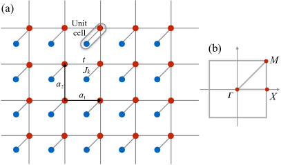
Figure 1: (a) Sketch of the square KLM with the nearest neighbor hopping $t$ and Kondo exchange coupling $J_{k}$: the conduction and localized orbitals are indicated by red and blue dots. (b) First Brillouin zone and its high symmetry points: $\Gamma=(0,0)$, $X=(\pi,0)$, and $M=(\pi,\pi)$.

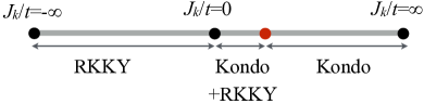
Figure 2: Conjectured ground state phase diagram for a square KLM at half filling. For $J_{k}/t>0$, a quantum critical point (red dot) separates the Kondo-screened and antiferromagnetically ordered phases. In the latter, the composite fermion spectral function is consistent with the coexistence of Kondo screening and the RKKY interaction; for $J_{k}/t<0$, the RKKY interaction is the only relevant energy scale.

III Composite fermion operator

To introduce the composite fermion operator, it is convenient to take a step back and assume that the KLM can be derived from a periodic Anderson model (PAM):

$$\hat{H}_{PAM} = \sum_{{\boldsymbol{k}},\sigma}\epsilon_{{\boldsymbol{k}}}{\hat{c}}^{\dagger}_{{\boldsymbol{k}},\sigma}{\hat{c}}_{{\boldsymbol{k}},\sigma}+V\sum_{{\boldsymbol{i}},\sigma}\big{(}\hat{c}^{\dagger}_{{\boldsymbol{i}},\sigma}\hat{f}^{\phantom{\dagger}}_{{\boldsymbol{i}},\sigma}+\text{H.c}\big{)}$$ (4)

$$+ \frac{U}{2}\sum_{{\boldsymbol{i}}}\big{(}\hat{n}_{{\boldsymbol{i}}}^{f}-1\big{)}^{2}.$$

The Hamiltonian $\hat{H}_{KLM}$ in Eq. (3) is obtained in the limit of strong Hubbard interaction $U$ on the $f$ orbitals by carrying out a canonical Schrieffer-Wolff Schrieffer and Wolff (1966) transformation of the PAM, $\hat{H}_{PAM}$. Hence, $e^{\hat{S}}$$\hat{H}_{PAM}$$e^{-\hat{S}}=\hat{H}_{KLM}$ with $\hat{S}^{\dagger}=-\hat{S}$. Then, the composite fermion operator is given by:

$$e^{\hat{S}}\hat{f}^{\dagger}_{{\boldsymbol{i}},\sigma^{\prime}}e^{-\hat{S}}\simeq\frac{2V}{U}\left({\hat{c}}^{\dagger}_{{\boldsymbol{i}},-\sigma^{\prime}}\hat{S}^{\sigma^{\prime}}_{{\boldsymbol{i}}}+\sigma^{\prime}{\hat{c}}^{\dagger}_{{\boldsymbol{i}},\sigma^{\prime}}\hat{S}^{z}_{\boldsymbol{i}}\right)\equiv\frac{2V}{U}\hat{\psi}^{\dagger}_{{\boldsymbol{i}},\sigma^{\prime}}.$$ (5)

In the above, it is understood that $\sigma^{\prime}$ takes the value $1$ ($-1$) for up (down) spin degrees of freedom, that $\hat{S}^{\sigma^{\prime}}_{{\boldsymbol{i}}}={\hat{f}}^{\dagger}_{{\boldsymbol{i}},\sigma^{\prime}}{\hat{f}}_{{\boldsymbol{i}},-\sigma^{\prime}}$ and that $\hat{S}^{z}_{{\boldsymbol{i}}}=\frac{1}{2}\sum_{\sigma^{\prime}}\sigma^{\prime}{\hat{f}}^{\dagger}_{{\boldsymbol{i}},\sigma^{\prime}}{\hat{f}}_{{\boldsymbol{i}},\sigma^{\prime}}$. This form matches that derived in Ref. Costi (2000) and a calculation of the former equation can be found in Ref. Raczkowski and Assaad (2019). An equivalent, but more transparent formulation is given in Ref. Maltseva et al. (2009) and reads:

$$\hat{\psi}^{\dagger}_{{\boldsymbol{i}},\sigma}=\sum_{\sigma^{\prime}}\hat{c}^{\dagger}_{{\boldsymbol{i}},\sigma^{\prime}}\boldsymbol{\sigma}_{\sigma^{\prime},\sigma}\cdot\hat{\boldsymbol{S}}_{\boldsymbol{i}}$$ (6)

where $\boldsymbol{\sigma}$ denotes the vector of Pauli spin matrices.

III.1 Symmetry properties of the composite fermion

As the composite fermion operator stems from a canonical transformation of the ${f}$-fermion operator, it must share identical symmetry properties. However, since the canonical transformation was carried out within perturbation theory, the statement is not exact and a calculation will show that the anti-commutation rules for the composite fermion operator read:

$$\big{\{}{\hat{\psi}}^{\dagger}_{\boldsymbol{i},\sigma},{\hat{\psi}}^{\phantom{\dagger}}_{\boldsymbol{j},\sigma^{\prime}}\big{\}}=\delta_{\boldsymbol{i},\boldsymbol{j}}\big{(}i\hat{\boldsymbol{S}}_{\boldsymbol{i}}\cdot\big{[}\big{(}\hat{\boldsymbol{c}}_{\boldsymbol{i}}^{\dagger}\boldsymbol{\sigma}\big{)}_{\sigma}\times\big{(}\boldsymbol{\sigma}\hat{\boldsymbol{c}}_{\boldsymbol{i}}^{\phantom{\dagger}}\big{)}_{\sigma^{\prime}}\big{]}$$

$$-\boldsymbol{\sigma}_{\sigma,\sigma^{\prime}}\cdot\hat{\boldsymbol{S}}_{\boldsymbol{i}}+\delta_{\sigma,\sigma^{\prime}}S(S+1)\big{)}$$ (7)

and

$$\big{\{}{\hat{\psi}}^{\dagger}_{\boldsymbol{i},\sigma},{\hat{\psi}}^{\dagger}_{\boldsymbol{j},\sigma^{\prime}}\big{\}}=\delta_{\boldsymbol{i},\boldsymbol{j}}\big{(}i\hat{\boldsymbol{S}}_{\boldsymbol{i}}\cdot\big{[}\big{(}\hat{\boldsymbol{c}}_{\boldsymbol{i}}^{\dagger}\boldsymbol{\sigma}\big{)}_{\sigma}\times\big{(}\boldsymbol{\sigma}\hat{\boldsymbol{c}}_{\boldsymbol{i}}^{\dagger}\big{)}_{\sigma^{\prime}}\big{]}\big{)}.$$ (8)

The above holds for the spin $S=1/2$ case. As a consequence the sum rule for a composite fermion spectral function defined as

$$A_{\psi}({\boldsymbol{k}},\omega)=-\frac{1}{\pi}\text{Im}G^{\text{r}et}_{\psi}({\boldsymbol{k}},\omega)$$ (9)

with

$$G^{\text{r}et}_{\psi}({\boldsymbol{k}},\omega)=-i\int^{\infty}_{0}dte^{i\omega t}\sum_{\sigma}\big{\langle}\big{\{}\hat{{\psi}}_{{\boldsymbol{k}},\sigma}(t),\hat{{\psi}}^{\dagger}_{{\boldsymbol{k}},\sigma}(0)\big{\}}\big{\rangle}$$ (10)

reads:

$$\int d\omega A_{\psi}({\boldsymbol{k}},\omega) =\sum_{\sigma}\big{\langle}\big{\{}\hat{{\psi}}^{\dagger}_{\boldsymbol{k},\sigma},\hat{{\psi}}^{\phantom{\dagger}}_{\boldsymbol{k},\sigma}\big{\}}\big{\rangle}$$

$$=-\frac{2}{N_{u}}\sum_{\boldsymbol{i}}\big{\langle}\hat{\boldsymbol{S}}_{\boldsymbol{i}}\cdot\hat{\boldsymbol{c}}^{\dagger}_{\boldsymbol{i}}\boldsymbol{\sigma}\hat{\boldsymbol{c}}^{\phantom{\dagger}}_{\boldsymbol{i}}\big{\rangle}+2S(S+1).$$

Since $-3/2<\langle\hat{\boldsymbol{S}}_{\boldsymbol{i}}\cdot\hat{\boldsymbol{c}}^{\dagger}_{\boldsymbol{i}}\boldsymbol{\sigma}\hat{\boldsymbol{c}}_{\boldsymbol{i}}\rangle<1/2$ the sum rule is, as expected, positive and is maximal for the antiferromagnetic alignment of impurity and conduction electron spins. Hence the sum rule lies in the interval $\left[0.5,4.5\right]$ and is hence very comparable to that of the conduction electron that takes a value of two.

We now show that the composite fermion transforms as an SU(2) spinor under global spin rotations. The generator for global spin rotations corresponds to the total spin:

$$\hat{\boldsymbol{S}}_{\text{tot}}=\sum_{\boldsymbol{i}}\big{(}\hat{\boldsymbol{S}}_{\boldsymbol{i}}+\frac{1}{2}\hat{\boldsymbol{c}}^{\dagger}_{\boldsymbol{i}}\boldsymbol{\sigma}\hat{\boldsymbol{c}}^{\phantom{\dagger}}_{\boldsymbol{i}}\big{)}$$ (12)

such that for

$$\hat{U}(\boldsymbol{e},\theta)=e^{-i\theta\boldsymbol{e}\cdot\hat{\boldsymbol{S}}_{\text{tot}}}$$ (13)

with $\boldsymbol{e}$ a unit vector in $\mathbb{R}^{3}$ and $\theta$ a real angle,

$$\hat{U}^{-1}(\boldsymbol{e},\theta)\hat{\boldsymbol{c}}^{\dagger}_{\boldsymbol{i}}\hat{U}(\boldsymbol{e},\theta)=\hat{\boldsymbol{c}}^{\dagger}_{\boldsymbol{i}}e^{i\frac{\theta}{2}\boldsymbol{e}\cdot\boldsymbol{\sigma}}$$ (14)

and

$$\hat{U}^{-1}(\boldsymbol{e},\theta)\hat{\boldsymbol{S}}_{\boldsymbol{i}}\hat{U}(\boldsymbol{e},\theta)=R(\boldsymbol{e},\theta)\hat{\boldsymbol{S}}_{\boldsymbol{i}}.$$ (15)

In the above, $R(\boldsymbol{e},\theta)$ is an SO(3) rotation around axis $\boldsymbol{e}$ with angle $\theta$. Since, $e^{i\frac{\theta}{2}\boldsymbol{e}\cdot\boldsymbol{\sigma}}\boldsymbol{\sigma}e^{-i\frac{\theta}{2}\boldsymbol{e}\cdot\boldsymbol{\sigma}}=R(\boldsymbol{e},\theta)\boldsymbol{\sigma}$, one will show that $\hat{\boldsymbol{\psi}}^{\dagger}_{\boldsymbol{i}}$ transforms as an SU(2) spinor:

$$\hat{U}^{-1}(\boldsymbol{e},\theta)\boldsymbol{\hat{\psi}}^{\dagger}_{\boldsymbol{i}}\hat{U}(\boldsymbol{e},\theta)=\boldsymbol{\hat{\psi}}^{\dagger}_{\boldsymbol{i}}e^{i\frac{\theta}{2}\boldsymbol{e}\cdot\boldsymbol{\sigma}}.$$ (16)

We will now discuss the behavior of the composite fermion spectral function upon neglecting vertex corrections in the large-$N$ and large-$S$ limits.

III.2 Omission of vertex contributions

Omitting vertex corrections, the composite fermion spectral function is given by a convolution of the spin susceptibility and the single particle spectral function. In particular, along the imaginary time, the bubble contribution to the correlation function reads:

$$\sum_{\sigma}\big{\langle}{\hat{\psi}}^{\phantom{\dagger}}_{\boldsymbol{i},\sigma}{\hat{\psi}}^{\dagger}_{\boldsymbol{j},\sigma}(\tau)\big{\rangle}=\sum_{\sigma}\big{\langle}\hat{\boldsymbol{S}}_{\boldsymbol{i}}\hat{\boldsymbol{S}}_{\boldsymbol{j}}(\tau)\big{\rangle}\big{\langle}\hat{c}^{\phantom{\dagger}}_{\boldsymbol{i},\sigma}\hat{c}^{\dagger}_{\boldsymbol{j},\sigma}(\tau)\big{\rangle}.$$ (17)

Transforming to real time and momentum space gives

$$A_{\psi}({\boldsymbol{k}},\omega)= \frac{1}{N_{u}}\sum_{\boldsymbol{p}}\int d\Omega A_{c}(\boldsymbol{p},\omega)\chi^{\prime\prime}(\boldsymbol{k}-\boldsymbol{p},\omega-\Omega)\times$$ (18)

$$\left[n_{B}(\omega-\Omega)-n_{F}(\Omega)\right].$$

In the above, $\chi^{\prime\prime}(\boldsymbol{k}-\boldsymbol{p},\omega-\Omega)$ corresponds to the imaginary part of the impurity spin susceptibility and $A_{c}(\boldsymbol{p},\omega)$ is the spectral function of the conduction electrons. $n_{B}(\omega-\Omega)$, $n_{F}(\omega)$ correspond respectively to the Bose-Einstein and Fermi-Dirac distributions at the considered temperature. Generically, the above convolution should yield a broad composite fermion spectral function. Consider for example a temperature scale where the spins are disordered such that the dynamical spin structure factor

$$S(\boldsymbol{q},\omega)=\chi^{\prime\prime}(\boldsymbol{q},\omega)n_{B}(\omega)$$ (19)

can be approximated by $S(\boldsymbol{q},\omega)\propto\delta(\omega)$, such that $\chi^{\prime\prime}(\boldsymbol{q},\omega)=0\,\,\forall\,\,\omega\neq 0$. In this case,

$$A_{\psi}({\boldsymbol{k}},\omega)\propto\frac{1}{N_{u}}\sum_{\boldsymbol{p}}A_{c}(\boldsymbol{p},\omega),$$ (20)

is $\boldsymbol{k}$-independent and corresponds to the density of states of the conduction electrons. We will see that our high temperature QMC data reproduce this form.

III.3 SU($N$) generalization and the large-$N$ limit

Here we generalize the SU(2) Kondo lattice model to SU($N$) in the totally antisymmetric self-conjugate representation. Let $T^{a}$ be the $N^{2}-1$ generators of SU($N$) that satisfy the normalization condition:

$$\mathop{\mathrm{Tr}}\left[T^{a}T^{b}\right]=\frac{1}{2}\delta_{a,b}.$$ (21)

For the SU(2) case, $T^{a}$ corresponds to the $\hat{T}=\frac{1}{2}\boldsymbol{\sigma}$ with $\boldsymbol{\sigma}$ a vector of the three Pauli spin matrices. The SU($N$) generalization of the KLM then reads:

$$\hat{H}^{N}_{KLM} = \sum_{{\boldsymbol{k}},\sigma=1}^{N}\epsilon_{{\boldsymbol{k}}}{\hat{c}}^{\dagger}_{{\boldsymbol{k}},\sigma}{\hat{c}}_{{\boldsymbol{k}},\sigma}+\frac{2J_{k}}{N}\sum_{{\boldsymbol{i}},a}\hat{T}_{{\boldsymbol{i}}}^{a,c}\hat{T}_{{\boldsymbol{i}}}^{a,f}.$$ (22)

where

$$\hat{T}^{a,c}_{{\boldsymbol{i}}}=\sum_{\sigma,\sigma^{\prime}=1}^{N}{\hat{c}}^{\dagger}_{{\boldsymbol{i}},\sigma}{T}^{a}_{\sigma,\sigma^{\prime}}{\hat{c}}^{\phantom{\dagger}}_{{\boldsymbol{i}},\sigma^{\prime}},\;\;\hat{T}^{a,f}_{{\boldsymbol{i}}}=\sum_{\sigma,\sigma^{\prime}=1}^{N}{\hat{f}}^{\dagger}_{{\boldsymbol{i}},\sigma}T^{a}_{\sigma,\sigma^{\prime}}{\hat{f}}^{\phantom{\dagger}}_{{\boldsymbol{i}},\sigma^{\prime}}.$$ (23)

The fermionic representation of the SU($N$) generators as well as the constraint

$$\sum_{\sigma=1}^{N}\hat{f}^{\dagger}_{{\boldsymbol{i}},\sigma}\hat{f}^{\phantom{\dagger}}_{{\boldsymbol{i}},\sigma}\equiv\hat{n}^{f}_{\boldsymbol{i}}=\frac{N}{2}$$ (24)

define the self-adjoint totally antisymmetric representation. To formulate the large-$N$ approximation, we use the relation:

$$\sum_{a}T^{a}_{\alpha,\beta}T^{a}_{\alpha^{\prime},\beta^{\prime}}=\frac{1}{2}\Big{(}\delta_{\alpha,\beta^{\prime}}\delta_{\alpha^{\prime},\beta}-\frac{1}{N}\delta_{\alpha,\beta}\delta_{\alpha^{\prime},\beta^{\prime}}\Big{)},$$ (25)

to show that in the constrained Hilbert space,

$$\frac{2J_{k}}{N}\sum_{a=1}^{N^{2}-1} \hat{T}^{a,c}_{{\boldsymbol{i}}}\hat{T}^{a,f}_{{\boldsymbol{i}}}=-\frac{J_{k}}{2N}\sum_{{\boldsymbol{i}}}\big{(}\hat{D}^{\dagger}_{{\boldsymbol{i}}}\hat{D}^{\phantom{\dagger}}_{{\boldsymbol{i}}}+\hat{D}^{\phantom{\dagger}}_{{\boldsymbol{i}}}\hat{D}^{\dagger}_{{\boldsymbol{i}}}\big{)}+\frac{J_{k}}{4}$$ (26)

with

$$\hat{D}^{\dagger}_{{\boldsymbol{i}}}=\sum_{\sigma=1}^{N}\hat{f}^{\phantom{\dagger}}_{{\boldsymbol{i}},\sigma}\hat{c}^{\dagger}_{{\boldsymbol{i}},\sigma}.$$

In the large-$N$ limit, $\hat{D}^{\dagger}_{{\boldsymbol{i}}}$ is of order $N$ and fluctuations around the mean-field are of order one, such that the square of the fluctuations can be neglected. The constraint, $\sum_{\sigma=1}^{N}\hat{f}^{\dagger}_{{\boldsymbol{i}},\sigma}\hat{f}^{\phantom{\dagger}}_{{\boldsymbol{i}},\sigma}$ is equally of order $N$ and since fluctuations around the mean are again of order one, it can be imposed on average.

The composite fermion operator is readily generalized to SU($N$) as:

$${\hat{\psi}}^{\dagger}_{{\boldsymbol{i}},\sigma}=\frac{4}{N}\sum_{\sigma^{\prime}=1}^{N}\sum_{a=1}^{N^{2}-1}\hat{c}^{\dagger}_{{\boldsymbol{i}},\sigma^{\prime}}T^{a}_{\sigma^{\prime},\sigma}\hat{T}^{a,f}_{{\boldsymbol{i}}}$$ (27)

where the pre-factor has to be chosen such that the above equation matches Eq. (2) at $N=2$. Using Eq. (25) and the constraint, we obtain

$$\hat{\psi}^{\dagger}_{{\boldsymbol{i}},\sigma}=\frac{2}{N}\big{[}\hat{f}^{\dagger}_{{\boldsymbol{i}},\sigma}\big{(}\hat{D}^{\dagger}_{{\boldsymbol{i}}}-\hat{f}^{\phantom{\dagger}}_{{\boldsymbol{i}},\sigma}\hat{c}^{\dagger}_{{\boldsymbol{i}},\sigma}\big{)}-\hat{c}^{\dagger}_{{\boldsymbol{i}},\sigma}\big{(}\hat{f}^{\dagger}_{{\boldsymbol{i}},\sigma}\hat{f}^{\phantom{\dagger}}_{{\boldsymbol{i}},\sigma}-1/2\big{)}\big{]}.$$ (28)

In the large-$N$ limit, $\hat{D}^{\dagger}_{{\boldsymbol{i}}}$ scales as $N$ and fluctuations of order one can be neglected such that

$${\hat{\psi}}^{\dagger}_{{\boldsymbol{i}},\sigma}\propto\hat{f}^{\dagger}_{{\boldsymbol{i}},\sigma}\frac{2}{N}\big{<}\hat{D}^{\dagger}_{{\boldsymbol{i}}}\big{>}.$$ (29)

In the heavy fermion state characterized by $\big{<}\hat{D}^{\dagger}_{{\boldsymbol{i}}}\big{>}\neq 0$ we expect the composite fermion operator to resolve the heavy fermion band since it is of dominant $f$-character.

Specifically, in the large-$N$ limit, the dispersion relation of the $f$-electron at finite hybridization $V=\frac{2}{N}\big{<}\hat{D}^{\dagger}_{{\boldsymbol{i}}}\big{>}=\frac{2}{N}\big{<}\hat{D}_{{\boldsymbol{i}}}\big{>}$ is given by

$$E_{{\boldsymbol{k}},\pm}=\frac{1}{2}\Big{(}\epsilon_{\boldsymbol{k}}\pm\sqrt{\epsilon^{2}_{\boldsymbol{k}}+J^{2}_{k}V^{2}}\Big{)}$$ (30)

with $\epsilon(\boldsymbol{k})=-2t\left(\cos{k_{x}}+\cos{k_{y}}\right)$. The $f$-electron spectral function $A_{f}({\boldsymbol{k}},\omega)=-\frac{1}{\pi}~{}\text{Im}~{}G^{\text{r}et}_{f}({\boldsymbol{k}},\omega)$ reads:

$$G^{\text{r}et}_{f}({\boldsymbol{k}},\omega)=\frac{|u_{\boldsymbol{k}}|^{2}}{\omega+i0^{+}-E^{-}_{{\boldsymbol{k}}}}+\frac{|v_{\boldsymbol{k}}|^{2}}{\omega+i0^{+}-E^{+}_{{\boldsymbol{k}}}}$$ (31)

with coherence factors:

$$|u_{\boldsymbol{k}}|^{2}=\frac{1}{2}\left(1+\frac{\epsilon_{\boldsymbol{k}}}{\sqrt{\epsilon^{2}_{\boldsymbol{k}}+(J_{k}V)^{2}}}\right),$$ (32)

$$|v_{\boldsymbol{k}}|^{2}=\frac{1}{2}\left(1-\frac{\epsilon_{\boldsymbol{k}}}{\sqrt{\epsilon^{2}_{\boldsymbol{k}}+(J_{k}V)^{2}}}\right).$$ (33)

Figure 3 plots $A_{f}({\boldsymbol{k}},\omega)$ as a function of energy and momentum. A dominant $f$-character of the low energy heavy fermion band can be noticed by thick black lines.

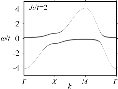
Figure 3: Spectral weight $A_{f}({\boldsymbol{k}},\omega)$ as a function of momentum ${\boldsymbol{k}}$ and energy $\omega/t$ for $J_{k}/t=2$ as obtained in the large-$N$ limit. The line thickness reflects the $f$-character of the band.

III.4 Strong coupling limit

An alternative way of understanding the composite fermion operator that becomes very transparent in the strong coupling limit, is in terms of bond operators between conduction electrons and spins Jurecka and Brenig (2001); Feldbacher et al. (2002). We consider the states:

$$\hat{s}^{\dagger}_{\boldsymbol{i}}\big{|}0\big{\rangle}=\frac{1}{\sqrt{2}}\left(\hat{c}^{\dagger}_{\boldsymbol{i},\uparrow}\hat{f}^{\dagger}_{\boldsymbol{i},\downarrow}-\hat{c}^{\dagger}_{\boldsymbol{i},\downarrow}\hat{f}^{\dagger}_{\boldsymbol{i},\uparrow}\right)\big{|}0\big{\rangle}$$

$$\hat{t}^{\dagger}_{\boldsymbol{i},0}\big{|}0\big{\rangle}=\frac{1}{\sqrt{2}}\left(\hat{c}^{\dagger}_{\boldsymbol{i},\uparrow}\hat{f}^{\dagger}_{\boldsymbol{i},\downarrow}+\hat{c}^{\dagger}_{\boldsymbol{i},\downarrow}\hat{f}^{\dagger}_{\boldsymbol{i},\uparrow}\right)\big{|}0\big{\rangle}$$

$$\hat{t}^{\dagger}_{\boldsymbol{i},\sigma}\big{|}0\big{\rangle}=\hat{c}^{\dagger}_{\boldsymbol{i},\sigma}\hat{f}^{\dagger}_{\boldsymbol{i},\sigma}\big{|}0\big{\rangle}$$

$$\hat{h}^{\dagger}_{\boldsymbol{i},\sigma}\big{|}0\big{\rangle}=\hat{f}^{\dagger}_{\boldsymbol{i},\sigma}\big{|}0\big{\rangle}$$

$$\hat{d}^{\dagger}_{\boldsymbol{i},\sigma}\big{|}0\big{\rangle}=\hat{c}^{\dagger}_{\boldsymbol{i},\uparrow}\hat{c}^{\dagger}_{\boldsymbol{i},\downarrow}\hat{f}^{\dagger}_{\boldsymbol{i},\sigma}\big{|}0\big{\rangle}.$$ (34)

Here, $\hat{s}^{\dagger}$ and $\hat{t}^{\dagger}_{1,0,-1}$ denote a singlet and three triplet states (triplons) with one conduction electron per site and $\hat{h}^{\dagger}_{\sigma}$ and $\hat{d}^{\dagger}_{\sigma}$ denote holons and doublons of the conduction electrons. We will assume that holons and doublons (singlets and triplets) are independent fermionic (bosonic) excitations such that $\{\hat{d}^{\#}_{\boldsymbol{i},\sigma},\hat{d}^{\#^{\prime}}_{\boldsymbol{j},\sigma^{\prime}}\}=\{\hat{h}^{\#}_{\boldsymbol{i},\sigma},\hat{h}^{\#^{\prime}}_{\boldsymbol{j},\sigma^{\prime}}\}=(1-\delta_{\#,\#^{\prime}})\delta_{\boldsymbol{i},\boldsymbol{j}}\delta_{\sigma,\sigma^{\prime}}$, $[\hat{t}_{\boldsymbol{i},m},\hat{t}^{\dagger}_{\boldsymbol{j},m^{\prime}}]=\delta_{\boldsymbol{i},\boldsymbol{j}}\delta_{m,m^{\prime}}$, $[\hat{s}_{\boldsymbol{i}},\hat{s}^{\dagger}_{\boldsymbol{j}}]=\delta_{\boldsymbol{i},\boldsymbol{j}}$ and $[\hat{t}_{\boldsymbol{i},m},\hat{t}_{\boldsymbol{j},m^{\prime}}]=[\hat{s}_{\boldsymbol{i}},\hat{s}_{\boldsymbol{j}}]=0$. Here $\#=\cdot,\dagger$, and the fermion and boson operators commute. To suppress the unphysical states, one then imposes the constraint:

$$\hat{s}^{\dagger}_{\boldsymbol{i}}\hat{s}_{\boldsymbol{i}}+\sum_{m=1,0,-1}\hat{t}^{\dagger}_{\boldsymbol{i},m}\hat{t}_{\boldsymbol{i},m}+\sum_{\sigma=\uparrow,\downarrow}(\hat{h}^{\dagger}_{\boldsymbol{i},\sigma}\hat{h}_{\boldsymbol{i},\sigma}+\hat{d}^{\dagger}_{\boldsymbol{i},\sigma}\hat{d}_{\boldsymbol{i},\sigma})=1.$$

In this representation the conduction electron and the composite fermion operators read:

$$\hat{c}^{\dagger}_{{\boldsymbol{i}},\sigma}=\frac{\sigma}{\sqrt{2}}(\hat{s}^{\dagger}_{\boldsymbol{i}}+\sigma\hat{t}^{\dagger}_{\boldsymbol{i},0})\hat{h}_{\boldsymbol{i},-\sigma}+\hat{t}^{\dagger}_{\boldsymbol{i},\sigma}\hat{h}_{\boldsymbol{i},\sigma}$$

$$-\frac{\hat{d}^{\dagger}_{\boldsymbol{i},\sigma}}{\sqrt{2}}(\hat{s}_{\boldsymbol{i}}-\sigma\hat{t}_{\boldsymbol{i},0})+\sigma\hat{d}^{\dagger}_{\boldsymbol{i},-\sigma}\hat{t}_{\boldsymbol{i},-\sigma}$$ (36)

$$2\hat{\psi}^{\dagger}_{{\boldsymbol{i}},\sigma}=-\frac{\sigma}{\sqrt{2}}(\hat{s}^{\dagger}_{\boldsymbol{i}}+\sigma\hat{t}^{\dagger}_{\boldsymbol{i},0})\hat{h}_{\boldsymbol{i},-\sigma}+(\hat{t}^{\dagger}_{\boldsymbol{i},\sigma}+2\hat{t}^{\dagger}_{\boldsymbol{i},-\sigma})\hat{h}_{{\boldsymbol{i}},\sigma}$$

$$-\frac{\hat{d}^{\dagger}_{\boldsymbol{i},\sigma}}{\sqrt{2}}(\hat{s}_{\boldsymbol{i}}-\sigma\hat{t}_{\boldsymbol{i},0})-\sigma d^{\dagger}_{\boldsymbol{i},-\sigma}(\hat{t}_{\boldsymbol{i},-\sigma}+2\hat{t}_{\boldsymbol{i},\sigma}).$$

As apparent both the conduction electron and composite fermion creation operators have very similar forms. In both cases a holon (triplon or singlet) can be annihilated to generate a triplon or singlet (doublon). We will now show that in the strong coupling limit, both the composite fermion and conduction electron spectral functions share the same features consisting of valence and conduction bands. In the limit $J_{k}\rightarrow\infty$ triplons can be neglected since in a given fixed particle number Hilbert space the triplon cost is set by $J_{k}$. Adopting this approximation,

$$2\hat{\psi}^{\dagger}_{{\boldsymbol{i}},\sigma}=-\frac{\sigma}{\sqrt{2}}\hat{s}^{\dagger}_{\boldsymbol{i}}\hat{h}_{\boldsymbol{i},-\sigma}-\frac{1}{\sqrt{2}}\hat{d}^{\dagger}_{\boldsymbol{i},\sigma}\hat{s}_{\boldsymbol{i}}$$ (38)

and the Hamiltonian reads:

$$\hat{H}_{KLM}= -\frac{t}{2}\sum_{\langle\boldsymbol{i},\boldsymbol{j}\rangle,\sigma}\left(\hat{s}^{\dagger}_{\boldsymbol{i}}\hat{h}_{\boldsymbol{i},-\sigma}\hat{h}^{\dagger}_{\boldsymbol{j},-\sigma}\hat{s}_{\boldsymbol{j}}+\hat{d}^{\dagger}_{\boldsymbol{i},\sigma}\hat{s}_{\boldsymbol{i}}\hat{s}^{\dagger}_{\boldsymbol{j}}\hat{d}^{\phantom{\dagger}}_{\boldsymbol{j},\sigma}+\text{H.c.}\right)$$ (39)

$$-\frac{3J_{k}}{4}\sum_{\boldsymbol{i}}\hat{s}^{\dagger}_{\boldsymbol{i}}\hat{s}^{\phantom{\dagger}}_{\boldsymbol{i}}.$$

In the above, we have neglected terms such as $\hat{d}^{\dagger}_{\boldsymbol{i},\sigma}\hat{h}^{\dagger}_{\boldsymbol{j},-\sigma}\hat{s}_{\boldsymbol{i}}\hat{s}_{\boldsymbol{j}}$ that create holon doublon excitations since these processes, in a given fixed particle-number Hilbert space, involve an excitation gap of $3J_{k}/2$. At $T=0$ and at half filling where the ground state corresponds to a product state of singlets, the retarded Green’s function reads:

$$4G^{\text{r}et}_{\psi}({\boldsymbol{k}},\omega) = \frac{1}{\omega-\left(\frac{3J_{k}}{4}+\frac{\epsilon(\boldsymbol{k})}{2}\right)+i0^{+}}$$ (40)

$$+ \frac{1}{\omega-\left(-\frac{3J_{k}}{4}+\frac{\epsilon(\boldsymbol{k})}{2}\right)+i0^{+}}$$

with $\epsilon(\boldsymbol{k})=-2t\left(\cos{k_{x}}+\cos{k_{y}}\right)$ the conduction electron dispersion relation. The valence and conduction bands are separated by an indirect gap since the maximal (minimal) energy of the valence (conduction) band is at $\boldsymbol{k}=(\pi,\pi)$ ($\boldsymbol{k}=(0,0)$). An equivalent form can be obtained for the conduction electron spectral function. The obtained dispersion relation compares with the strong coupling expansion presented in Ref. Tsunetsugu et al. (1997).

III.5 Large-$S$ limit

We now consider the large-$S$ limit. Here we systematically enhance the dimension of the representation of the SU(2) group of the impurity spins such that the Hamiltonian is identical to that of Eq. (3) but with

$$\hat{\boldsymbol{S}}_{{\boldsymbol{i}}}^{2}=S(S+1)$$ (41)

for half integer spins. Since we are working on bipartite lattices, we foresee antiferromagnetic order and choose the following Holstein-Primakov representation of the spin algebra on the A

$$\hat{S}^{z}_{{\boldsymbol{i}}}=S-\hat{b}^{\dagger}_{{\boldsymbol{i}}}\hat{b}^{\phantom{\dagger}}_{{\boldsymbol{i}}},\,\,\hat{S}^{+}_{{\boldsymbol{i}}}=\sqrt{2S-\hat{b}^{\dagger}_{{\boldsymbol{i}}}\hat{b}^{\phantom{\dagger}}_{{\boldsymbol{i}}}}\,\hat{b}^{\phantom{\dagger}}_{{\boldsymbol{i}}}$$ (42)

and B sub-lattices

$$\hat{S}^{z}_{{\boldsymbol{i}}}=\hat{b}^{\dagger}_{{\boldsymbol{i}}}\hat{b}^{\phantom{\dagger}}_{{\boldsymbol{i}}}-S,\,\,\hat{S}^{+}_{{\boldsymbol{i}}}=\hat{b}^{\dagger}_{{\boldsymbol{i}}}\sqrt{2S-\hat{b}^{\dagger}_{{\boldsymbol{i}}}\hat{b}^{\phantom{\dagger}}_{{\boldsymbol{i}}}}.$$ (43)

The Néel state corresponds to the vacuum of the boson operator $\hat{b}_{{\boldsymbol{i}}}$. Hence in the large-$S$ limit and in the Néel state we will assume that $\langle\hat{b}^{\dagger}_{{\boldsymbol{i}}}\hat{b}^{\phantom{\dagger}}_{{\boldsymbol{i}}}\rangle<<2S$ allowing one to expand the square root. With this approximation, and including the RKKY interaction,

$$J_{RKKY}\sum_{\left<{\boldsymbol{i}},{\boldsymbol{j}}\right>}\hat{\boldsymbol{S}}_{\boldsymbol{i}}\cdot\hat{\boldsymbol{S}}_{\boldsymbol{j}}$$ (44)

to the KLM, we obtain:

$$\hat{H}= \sum_{{\boldsymbol{k}},\sigma}\epsilon_{{\boldsymbol{k}}}{\hat{c}}^{\dagger}_{{\boldsymbol{k}},\sigma}\hat{c}_{{\boldsymbol{k}},\sigma}+\frac{J_{k}}{2}S\sum_{{\boldsymbol{i}}}e^{i\boldsymbol{Q}\cdot\boldsymbol{i}}\hat{\boldsymbol{c}}^{\dagger}_{{\boldsymbol{i}}}\boldsymbol{\sigma}^{z}\hat{\boldsymbol{c}}_{{\boldsymbol{i}}}+$$

$$+ \frac{J_{RKKY}S}{2}\sum_{{\boldsymbol{i}},\boldsymbol{\delta}}\big{(}2\hat{b}^{\dagger}_{{\boldsymbol{i}}}\hat{b}^{\phantom{\dagger}}_{{\boldsymbol{i}}}+\hat{b}^{\phantom{\dagger}}_{{\boldsymbol{i}}}\hat{b}^{\phantom{\dagger}}_{{\boldsymbol{i}}+\boldsymbol{\delta}}+\hat{b}^{\dagger}_{{\boldsymbol{i}}}\hat{b}^{\dagger}_{{\boldsymbol{i}}+\boldsymbol{\delta}}\big{)}$$

$$+ J_{k}\sqrt{\frac{S}{2}}\sum_{{\boldsymbol{i}}\in A}\big{(}\hat{c}^{\dagger}_{{\boldsymbol{i}},\uparrow}\hat{c}^{\phantom{\dagger}}_{{\boldsymbol{i}},\downarrow}\hat{b}_{{\boldsymbol{i}}}^{\dagger}+\mathrm{H.c.}\big{)}+$$

$$+ J_{k}\sqrt{\frac{S}{2}}\sum_{{\boldsymbol{i}}\in B}\big{(}\hat{c}^{\dagger}_{{\boldsymbol{i}},\uparrow}\hat{c}^{\phantom{\dagger}}_{{\boldsymbol{i}},\downarrow}\hat{b}_{{\boldsymbol{i}}}^{\phantom{\dagger}}+\mathrm{H.c.}\big{)}+\cdots.$$ (45)

In the above, the ellipsis corresponds to terms in lower order in $S$, $\boldsymbol{\delta}$ runs over the nearest neighbors of a given site, and $e^{i\boldsymbol{Q}\cdot\boldsymbol{i}}$ takes the value $1$ ($-1$) on the A (B) sub-lattice.

We now turn our attention to the composite fermion operator. Using the Holstein-Primakov representation we obtain:

$$\hat{\boldsymbol{\psi}}^{\dagger}_{{\boldsymbol{i}}}= S\hat{\boldsymbol{c}}^{\dagger}_{{\boldsymbol{i}}}\sigma^{z}e^{i\boldsymbol{Q}\cdot\boldsymbol{i}}+\sqrt{\frac{S}{2}}\hat{\boldsymbol{c}}^{\dagger}_{{\boldsymbol{i}}}\frac{1+e^{i\boldsymbol{Q}\cdot\boldsymbol{i}}}{2}\big{(}\sigma^{+}\hat{b}^{\dagger}_{{\boldsymbol{i}}}+\sigma^{-}\hat{b}^{\phantom{\dagger}}_{{\boldsymbol{i}}}\big{)}$$

$$+ \sqrt{\frac{S}{2}}\hat{\boldsymbol{c}}^{\dagger}_{{\boldsymbol{i}}}\frac{1-e^{i\boldsymbol{Q}\cdot\boldsymbol{i}}}{2}\big{(}\sigma^{+}\hat{b}^{\phantom{\dagger}}_{{\boldsymbol{i}}}+\sigma^{-}\hat{b}^{\dagger}_{{\boldsymbol{i}}}\big{)}+\cdots.$$ (46)

In the above the ellipsis again refers to lower order terms in $S$ and $\sigma^{\pm}=\sigma^{x}\pm i\sigma^{y}$. Retaining terms only up to order $S$, the Hamiltonian of Eq. (45) corresponds to electrons subject to a static staggered magnetic field of magnitude $J_{k}S$ in the $z$-direction as well as spin waves. The composite fermion operator reduces to the conduction electron operator with a phase shift such that

$$\sum_{\sigma}\big{\langle}\hat{{\psi}}^{\phantom{\dagger}}_{{\boldsymbol{i}},\sigma}(0)\hat{{\psi}}^{\dagger}_{{\boldsymbol{j}},\sigma}(\tau)\big{\rangle}= S^{2}\sum_{\sigma}\big{\langle}\hat{c}^{\phantom{\dagger}}_{{\boldsymbol{i}},\sigma}(0)\hat{c}^{\dagger}_{{\boldsymbol{j}},\sigma}(\tau)\big{\rangle}e^{i\boldsymbol{Q}\cdot(\boldsymbol{j}-\boldsymbol{i})}$$

$$+ \cdots.$$ (47)

Hence in the large-$S$ limit, the composite fermion Green’s function should correspond to the $c$-Green’s function with a momentum shift of $\boldsymbol{Q}$. We note that the above equation can also be motivated from Eq. (17) with $\langle\hat{\boldsymbol{S}}_{i}\hat{\boldsymbol{S}}_{j}(\tau)\rangle\propto S^{2}e^{i\boldsymbol{Q}\cdot(\boldsymbol{j}-\boldsymbol{i})}$ as appropriate for a long ranged antiferromagnetic state.

IV Quantum Monte Carlo

We consider the SU($N$) generalization of the Kondo lattice Hamiltonian given in Eq. (3):

$$\hat{H} = \hat{H}_{t}-\frac{J_{k}}{4N}\sum_{\boldsymbol{i}}\Big{\{}\big{(}\boldsymbol{\hat{c}}^{\dagger}_{\boldsymbol{i}}\boldsymbol{\hat{f}}_{\boldsymbol{i}}+\mathrm{H.c.}\big{)}^{2}+\big{(}i\boldsymbol{\hat{c}}^{\dagger}_{\boldsymbol{i}}\boldsymbol{\hat{f}}_{\boldsymbol{i}}+\mathrm{H.c.}\big{)}^{2}\Big{\}}$$ (48)

$$+\frac{U}{N}\sum_{\boldsymbol{i}}\Big{(}\boldsymbol{\hat{f}}^{\dagger}_{\boldsymbol{i}}\boldsymbol{\hat{f}}_{\boldsymbol{i}}-\frac{1}{2}\Big{)}^{2}$$

where $\hat{H}_{t}=-t\sum_{\langle\boldsymbol{i},\boldsymbol{j}\rangle}(\boldsymbol{\hat{c}}^{\dagger}_{\boldsymbol{i}}\boldsymbol{\hat{c}}_{\boldsymbol{j}}+\mathrm{H.c.})$ and $\boldsymbol{\hat{c}}^{\dagger}_{\boldsymbol{i}}$ and $\boldsymbol{\hat{f}}^{\dagger}_{\boldsymbol{i}}$ are $N$ flavor fermion operators. Since the Monte Carlo sampling is formulated in an unconstrained Hilbert space, to impose the constraint Eq. (24) we have added above a Hubbard-$U$ interaction acting on the $f$-electrons. Importantly, the Hubbard interaction commutes with the Hamiltonian such that the constraint is very efficiently implemented.

Next, using the Hubbard-Stratonovich transformation the partition function can be written as:

$$Z~{}\equiv~{}\int\mathcal{D}\{z,\mathcal{\lambda}\}~{}e^{-N\mathcal{S}\{z,\mathcal{\lambda}\}}$$ (49)

with the action

$$\mathcal{S}\{z,\lambda\} = -\ln\Big{[}~{}\mbox{Tr}~{}\mathcal{T}e^{-\int^{\beta}_{0}d\tau~{}\hat{H}\{z,\lambda\}}\Big{]}$$

$$+\int^{\beta}_{0}d\tau\sum_{\boldsymbol{i}}\Big{\{}\frac{J_{k}}{4}|z(\boldsymbol{i},\tau)|^{2}+\frac{U}{4}|\lambda(\boldsymbol{i},\tau)|^{2}\Big{\}}$$

and time dependent Hamiltonian

$$\hat{H}\{z,\lambda\} = \hat{H}_{t}+\sum_{\boldsymbol{i}}\Big{\{}-\frac{J_{k}}{2}\big{(}z(\boldsymbol{i},\tau)\boldsymbol{\hat{c}}^{\dagger}_{\boldsymbol{i}}\boldsymbol{\hat{f}}_{\boldsymbol{i}}+\mathrm{H.c.}\big{)}$$ (51)

$$-iU\lambda(\boldsymbol{i},\tau)\Big{(}\boldsymbol{\hat{f}}^{\dagger}_{\boldsymbol{i}}\boldsymbol{\hat{f}}_{\boldsymbol{i}}-\frac{1}{2}\Big{)}\Big{\}}.$$

In the above scalar field $\mathcal{\lambda}(\boldsymbol{i},\tau)$ enforces the constraint and $z(\boldsymbol{i},\tau)$ is a space and time dependent complex bond field. For a particle-hole symmetric band the imaginary part of the action takes the value $n\pi$ with $n$ an integer resulting in no negative sign problem for even $N$ Assaad (1999); Capponi and Assaad (2001); Raczkowski and Assaad (2020). Note that the on-site Hubbard term commutes with the Hamiltonian. Hence for a given $U$ and inverse temperature $\beta$ the unphysical even-parity states are suppressed by a factor $e^{-\beta U/N}$. The choice $\beta U/N(\geq 10)$ allows restriction of the Hilbert space to the odd parity sector within our error bars.

We have used both the finite temperature Blankenbecler et al. (1981); White et al. (1989) as well as the zero temperature auxiliary field QMC methods Assaad (1999); Assaad and Evertz (2008); Bercx et al. (2017). For the SU(2) invariant KLM we have mainly used the finite temperature algorithm. In that case, it is possible to perform simulations at low enough temperatures to address the interplay between strong antiferromagnetic spin correlations and Kondo screening. Given that the RKKY scale varies as $1/N$ in the SU($N$) generalization of the KLM, we have opted for $N>2$ for a projective QMC technique based on the imaginary-time evolution of a trial wave function $|\Psi_{\text{T}}\rangle$, with $\langle\Psi_{\text{T}}|\Psi_{0}\rangle\neq 0$, to the ground state $|\Psi_{0}\rangle$:

$$\frac{\langle\Psi_{0}|\hat{O}|\Psi_{0}\rangle}{\langle\Psi_{0}|\Psi_{0}\rangle}=\lim_{\Theta\rightarrow\infty}\frac{\langle\Psi_{\text{T}}|e^{-\Theta\hat{\mathcal{H}}}\hat{O}e^{-\Theta\hat{\mathcal{H}}}|\Psi_{\text{T}}\rangle}{\langle\Psi_{\text{T}}|e^{-2\Theta\hat{\mathcal{H}}}|\Psi_{\text{T}}\rangle}$$ (52)

where the projection parameter $\Theta$ is chosen to be sufficiently large (up to $2\Theta t=400$ for our largest $N=8$) to reach the antiferromagnetic ground state even at a small value of $J_{k}/t=0.4$. Finally, taking into account the phase diagram presented in Refs. Assaad (1999); Capponi and Assaad (2001); Raczkowski and Assaad (2020) we have considered values of $J_{k}/t$ representative of both the magnetically ordered RKKY and disordered Kondo screened phases.

The SU($N$) KLM is one of the standard Hamiltonians implemented in the ALF2.0 library ALF Collaboration et al. (2020). We have used this library to produce our results and refer the reader to Ref. ALF Collaboration et al. (2020) for further details of the implementation. We also note that the measurement of the composite fermion time displaced correlation functions is implemented in ALF2.0 so that no add-ons to the library are required to reproduce the data presented in this paper.

V Quantum Monte Carlo results

Our main goal is to compute the momentum resolved composite fermion spectral function defined in Eqs. (9) - (10). The motivation of doing so stems from the fact that the low energy heavy fermion band has predominantly $f$-character and thus the composite fermion Eq. (2) may provide a better possibility to resolve heavy quasiparticles as compared with the spectral function on conduction electrons, $A_{c}({\boldsymbol{k}},\omega)=-\frac{1}{\pi}~{}\text{Im}~{}G^{\text{r}et}_{c}({\boldsymbol{k}},\omega)$, where

$$G^{\text{r}et}_{c}({\boldsymbol{k}},\omega)=-i\int^{\infty}_{0}dte^{i\omega t}\sum_{\sigma}\big{\langle}\big{\{}{\hat{c}}_{{\boldsymbol{k}},\sigma}(t),{\hat{c}}^{\dagger}_{{\boldsymbol{k}},\sigma}(0)\big{\}}\big{\rangle}.$$

To extract the real frequency data from the imaginary time data of QMC we have used the stochastic analytical continuation algorithm Beach (2004) of the ALF2.0 ALF Collaboration et al. (2020) library. In the following we present and discuss our results considering separately antiferromagnetic $J_{k}/t>0$ and ferromagnetic $J_{k}/t<0$ exchange couplings.

V.1 Antiferromagnetic Kondo lattice

As proposed by Doniach Doniach (1977), the antiferromagnetic Kondo coupling in the KLM leads to two energy scales set by Kondo and RKKY exchange interactions. The Kondo scale is given by a single impurity Kondo scale $T_{k}\sim We^{-W/J_{k}}$, where $W$ denotes the bandwidth of the conduction electrons. The RKKY scale is given by $J_{RKKY}(\boldsymbol{q})=J^{2}_{k}\chi^{c}(\boldsymbol{q},\omega=0)$ where $\chi^{c}$ is the spin susceptibility of the conduction electrons. Depending on the magnitude of the exchange coupling, the physics is dominated by one of these two energy scales. For large Kondo couplings, the Kondo effect is the dominant effect and stabilizes the spin-gapped Kondo singlet phase. For small Kondo couplings, the RKKY interaction is the largest scale and thus magnetic order of local moments occurs. This competition leads to a quantum phase transition which for the SU(2) KLM on the square lattice is shown to arise at the critical point $J^{c}_{k}/t\simeq 1.45$ Assaad (1999); Capponi and Assaad (2001). The location of the magnetic transition shifts with increasing number of flavors $N$ in the SU($N$) generalization of the KLM towards smaller values of $J_{k}/t$ Raczkowski and Assaad (2020). Keeping in mind these two competing energy scales, we proceed to discuss their signature in the momentum resolved composite fermion spectral function $A_{\psi}({\boldsymbol{k}},\omega)$. By comparing the latter with the single particle spectrum of conduction electrons $A_{c}({\boldsymbol{k}},\omega)$ we will directly show the advantage of usage of $A_{\psi}({\boldsymbol{k}},\omega)$ in detecting the existence of heavy quasiparticles especially in the weak coupling region of the phase diagram.

V.1.1 SU(2) Kondo lattice model

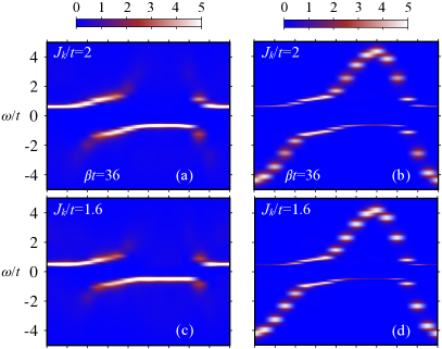
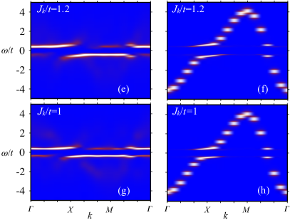
Figure 4: Composite fermion $A_{\psi}({\boldsymbol{k}},\omega)$ (left) and conduction electron $A_{c}({\boldsymbol{k}},\omega)$ (right) spectral functions in the $12\times 12$ KLM at $\beta t=36$ with: (a,b) $J_{k}/t=2$; (c,d) $J_{k}/t=1.6$; (e,f) $J_{k}/t=1.2$, and (g,h) $J_{k}/t=1$.

We start with finite but low temperature $T=t/36$ data of the SU(2) invariant KLM in the Kondo-screened phase. The Kondo-screened phase is adiabatically connected to the strong coupling limit, where each spin binds with a conduction electron into a spin singlet. As discussed in Sec. III.4, the composite fermion spectral function $A_{\psi}({\boldsymbol{k}},\omega)$ should show a well defined quasiparticle band. Figures 4(a) with $J_{k}/t=2$ and  4(c) with $J_{k}/t=1.6$ confirm this point of view. Furthermore, although no actual symmetry breaking occurs in the QMC simulations, the low energy excitation spectrum is consistent with that found in a simple large-$N$ picture in which the hybridization gap opens up in the presence of a finite hybridization parameter $V$, see Fig. 3. Given the sum rule $|u_{\boldsymbol{k}}|^{2}+|v_{\boldsymbol{k}}|^{2}=1$ of mean-field coherence factors defined in Eqs. (32) and (33), the low energy part of the spectrum with the dominant $f$-character is poorly represented in the large-$N$ conduction electron spectral function $A_{c}({\boldsymbol{k}},\omega)$. As is apparent in Figs. 4(b) and 4(d) the same holds for the QMC data: the intensity of a weakly dispersive heavy fermion band in $A_{c}({\boldsymbol{k}},\omega)$ quickly drops upon approaching the $M$ point while being much more pronounced in the composite fermion spectral function $A_{\psi}({\boldsymbol{k}},\omega)$.

To illustrate further a superior quality of the composite fermion as a tool in tracing heavy fermon excitations, we plot in Figs. 4(e) and 4(g) its spectra in the RKKY dominated part of the phase diagram with $J_{k}/t=1.2$ and $J_{k}/t=1$. To make sure that the used temperature $T=t/36$ is low enough to access the interplay between Kondo screening and the RKKY interaction, we plot in Fig. 5 the corresponding temperature dependence of a static spin structure factor

$$S({\boldsymbol{Q}})=\frac{1}{N_{u}}\sum_{{\boldsymbol{i}},{\boldsymbol{j}}}e^{-i{\boldsymbol{Q}}({\boldsymbol{i}}-{\boldsymbol{j}})}\langle\hat{S}^{z}_{\boldsymbol{i}}\hat{S}^{z}_{\boldsymbol{j}}\rangle$$ (54)

at the antiferromagnetic wave vector ${\boldsymbol{Q}}=(\pi,\pi)$. As can be seen, the onset of antiferromagnetic fluctuations begins already around $T=t/12$. Nevertheless, we easily note in $A_{\psi}({\boldsymbol{k}},\omega)$ the continued existence of the flat heavy fermion band around the $M$, in striking contrast with its barely visible fingerprint in the $c$-electron spectra, see Figs. 4(f) and 4(h).

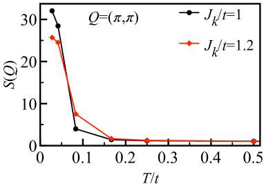
Figure 5: Static spin structure factor $S({\boldsymbol{Q}})$ at ${\boldsymbol{Q}}=(\pi,\pi)$ for the localized spins as a function of temperature $T/t$.

A closer inspection of $A_{\psi}({\boldsymbol{k}},\omega)$ reveals additional low energy band features located near the $\Gamma$ ($M$) momentum in the lower $\omega/t<0$ (upper $\omega/t>0$) part of the spectrum, respectively. These shadow features emerge from the scattering of the heavy quasiparticle off the magnetic fluctuations with the wave vector ${\boldsymbol{Q}}=(\pi,\pi)$. Another consequence of strong antiferromagnetic spin correlations seen in $A_{\psi}({\boldsymbol{k}},\omega)$ is a faint image of the $c$-electron band with a momentum shift of $\boldsymbol{Q}$, see Fig. 4(g). The emergence of this feature becomes clear by considering a simplified form of the composite fermion Green’s function in Eq. (III.5) valid in the large-$S$ limit.

Altogether, our finite-$T$ spectral data point towards the coexistence of Kondo screening and antiferromagnetism also in the broken spin symmetry phase that occurs at $T=0$. We will confirm using the projective QMC method in Sec. V.1.2 that this conjecture remains valid down to our smallest considered value $J_{k}/t=0.4$.

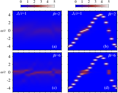
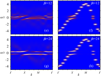
Figure 6: Emergence of the heavy fermion band structure as seen in $A_{\psi}({\boldsymbol{k}},\omega)$ (left) and $A_{c}({\boldsymbol{k}},\omega)$ (right) upon decreasing temperature in the $12\times 12$ KLM at $J_{k}/t=1$: (a,b) $\beta t=2$; (c,d) $\beta t=6$; (e,f) $\beta t=12$, and (g,h) $\beta t=24$.

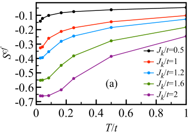
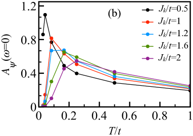
Figure 7: (a) Local spin-spin correlation function $S^{cf}=\tfrac{1}{N_{u}}\sum_{{\boldsymbol{i}}}\langle\hat{\boldsymbol{S}}^{c}_{{\boldsymbol{i}}}\cdot\hat{\boldsymbol{S}}_{{\boldsymbol{i}}}\rangle$ and (b) estimate of the local density of states at the Fermi level $A_{\psi}(\omega=0)\approx\tfrac{1}{\pi}\tfrac{\beta}{N_{u}}\sum_{{\boldsymbol{k}}}G_{\psi}({\boldsymbol{k}},\tau=\beta/2)$ as a function of temperature $T/t$ and for various Kondo couplings $J_{k}/t$. The formation of local singlets seen as a decrease in $S^{cf}$ induces a depletion of the spectral weight and opens a gap in $A_{\psi}(\omega=0)$ in the low-$T$ limit.

We turn now to the discussion of how the electronic states in $A_{\psi}({\boldsymbol{k}},\omega)$ emerge and rearrange on passing through progressively lower energy scales upon cooling the system. For concreteness, let us focus on the $J_{k}/t=1$ case illustrated in Fig. 6. In the high temperature limit, it is legitimate to expect that the local moments do not interact with the spin degrees of freedom of the conduction electrons and are fully disordered. Consequently, $A_{\psi}({\boldsymbol{k}},\omega)$ should have a $\boldsymbol{k}$-independent form given by the density of states of the conduction electrons, see Eq. (20). This is precisely observed in Fig. 6(a) at $T=t/2$: a faint featureless cloud of the composite spectral weight is discernible only in a narrow window around the Fermi level reflecting the saddle point in $A_{c}({\boldsymbol{k}},\omega)$. As shown in Fig. 6(b), the latter approaches that of the tight-binding model with the van Hove singularity in the density of states at $\omega=0$ yielding in turn the strongest signal in $A_{\psi}({\boldsymbol{k}},\omega\simeq 0)$.

Upon lowering $T$, the screening of magnetic impurities becomes progressively important as signaled by a decreasing behavior of the local spin-spin correlation function $S^{cf}=\tfrac{1}{N_{u}}\sum_{{\boldsymbol{i}}}\langle\hat{\boldsymbol{S}}^{c}_{{\boldsymbol{i}}}\cdot\hat{\boldsymbol{S}}_{{\boldsymbol{i}}}\rangle$, see Fig. 7(a). The formation of bound states between conduction electrons and the $f$-spins gives rise to quasiparticle poles in the composite fermion Green’s function. As a result, the hybridized band structure becomes apparent in $A_{\psi}({\boldsymbol{k}},\omega)$, see Figs. 6(c) and  6(e), with a concomitant suppression of the conduction electron spectral weight at the Fermi level. Finally, around $T=t/24$, $S^{cf}$ begins to saturate and thus the sum rule for the composite fermion spectral weight in Eq. (III.1) attains its maximum. As seen in Fig. 6(g), $A_{\psi}({\boldsymbol{k}},\omega)$ is exhausted mainly by the intense heavy fermion band while the rest of the weight forms the shadow features.

We conclude this section with pointing out that the crossover from free to screened magnetic impurities at low $T$ can be equally resolved in local density of states at the Fermi level $A_{\psi}(\omega=0)$. This quantity is directly related to the zero-bias differential conductance $dI_{(V=0)}/dV$ in STM experiments. We compute it using an approximate form

$$A_{\psi}(\omega=0)\approx\frac{1}{\pi}\frac{\beta}{N_{u}}\sum_{{\boldsymbol{k}}}G_{\psi}({\boldsymbol{k}},\tau=\beta/2)$$ (55)

and plot its temperature dependence in Fig. 7(b). As is apparent, the formation of local singlets induces a depletion of the spectral weight and opens a gap in $A_{\psi}(\omega=0)$ in the low-$T$ limit. We confirm this in Fig. 8 which plots the temperature evolution of a momentum integrated composite fermion spectral function $A_{\psi}(\omega)=\tfrac{1}{N_{u}}\sum_{{\boldsymbol{k}}}A_{\psi}({\boldsymbol{k}},\omega)$ obtained with the analytical continuation of the imaginary time QMC data. By lowering temperature one observes first an enhancement of the weight at the Fermi level followed, below $T=t/6$, by its transfer to symmetrically developed about $\omega=0$ finite frequency peaks. In combination with the momentum resolved data in Fig. 6(g), the sharp peaks at the lowest $T=t/24$ can be identified as upper and lower heavy fermion bands.

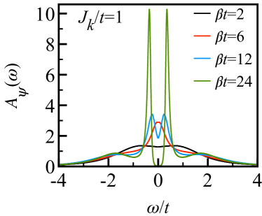
Figure 8: Temperature evolution of the momentum integrated composite fermion spectral function $A_{\psi}(\omega)=\tfrac{1}{N_{u}}\sum_{{\boldsymbol{k}}}A_{\psi}({\boldsymbol{k}},\omega)$ at $J_{k}/t=1$.

V.1.2 SU($N$) Kondo lattice model

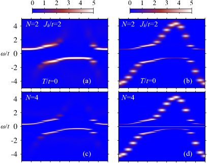
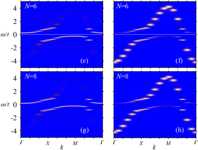
Figure 9: Composite fermion $A_{\psi}({\boldsymbol{k}},\omega)$ (left) and conduction electron $A_{c}({\boldsymbol{k}},\omega)$ (right) spectral functions at $T=0$ of the $12\times 12$ SU($N$) KLM in the Kondo-screened phase at $J_{k}/t=2$: (a,b) $N=2$; (c,d) $N=4$; (e,f) $N=6$, and (g,h) $N=8$.

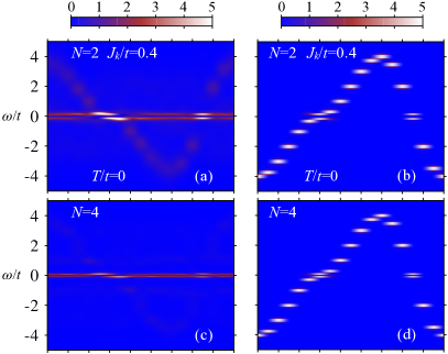
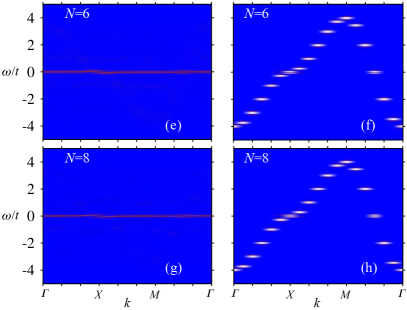
Figure 10: Same as in Fig. 9 but in the magnetically ordered phase at $J_{k}/t=0.4$.

We proceed now to discuss spectral properties of the composite fermion in the SU($N$) generalization of the KLM. Figures 9(a) and 9(b) plot the zero temperature $A_{\psi}({\boldsymbol{k}},\omega)$ and $A_{c}({\boldsymbol{k}},\omega)$ spectra for $N=2$ obtained in the Kondo insulating phase at $J_{k}/t=2$. Comparing with the corresponding finite-$T$ data, one easily recognizes the main spectral features whose momentum and frequency dependence as well as the intensity match well those found at $T=t/36$, see Figs. 4(a) and 4(b). Furthermore, we note that increasing $N$ has a double effect, see Figs. 9(c)-9(h): (i) the quasiparticle gap is reduced, and (ii) overall, both the $A_{\psi}({\boldsymbol{k}},\omega)$ and $A_{c}({\boldsymbol{k}},\omega)$ spectra become more coherent. This is a natural result given that larger $N$: (i) enhances the domain of stability of a magnetically disordered Kondo phase Raczkowski and Assaad (2020) bringing its description in line with a strong coupling picture, and (ii) reduces the effect of antiferromagnetic spin fluctuations on the self-energy such that it approaches the $\boldsymbol{k}$ independent large-$N$ limit.

We have equally plotted both $A_{\psi}({\boldsymbol{k}},\omega)$ and $A_{c}({\boldsymbol{k}},\omega)$ at smaller values of $J_{k}/t=0.4$ as a function of $N$. This coupling strength is located in the phase diagram deeply in the antiferromagnetically ordered phase. As evident in Fig. 10(a), the composite fermion spectrum $A_{\psi}({\boldsymbol{k}},\omega)$ at $N=2$ shares aspects of the large-$N$ and large-$S$ limits. On the one hand, one observes a low energy flat heavy fermion band with a renormalized weight accompanied by the shadow bands around the $\Gamma$ and $M$ momenta. These shadows display roughly the same intensity as the original heavy quasiparticles, thus reflecting robust magnetic order. On the other hand, a nearly fully polarized staggered magnetic moment results in a pronounced image of the $c$-band consistent with the large-$S$ limit. This image looses its intensity at larger $N$, see Figs. 10(c), 10(e), and 10(g). Seemingly, that could be a consequence of a reduced, as a function of growing values of $N$, distance to the magnetic order-disorder transition point that scales as $J_{c}(N)\propto\frac{1}{\ln(N)}$ Raczkowski and Assaad (2020). However, given that the $f$-local moment was found in Ref. Raczkowski and Assaad (2020) to be next to saturated at $J_{k}/t=0.4$ for each considered $N$, we find it more appropriate to assume that the loss in intensity originates from the scattering between a growing number of Goldstone modes associated with the SU($N$) spin symmetry breaking in the Néel phase. This produces relatively broad spin wave excitations seen in the dynamical spin structure factor Raczkowski and Assaad (2020), clearly beyond the lowest order approximation in $S$ that leads us to a simplified form of the composite fermion Green’s function in Eq. (III.5). Strictly speaking, large-$S$ theory does not apply here and one should use flavor wave theory as done in Ref. Kim et al. (2017).

In stark contrast to $A_{\psi}({\boldsymbol{k}},\omega)$, the corresponding conduction electron spectra $A_{c}({\boldsymbol{k}},\omega)$, see right panels of Fig. 10, display merely a direct hybridization gap without any discernible signature of the heavy fermion band. As we argue below, due to its extremely low intensity, the latter can only be resolved on a logarithmic scale.

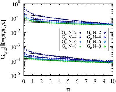
Figure 11: Zero temperature composite fermion $G_{\psi}(\boldsymbol{k},\tau)$ and conduction electron $G_{c}(\boldsymbol{k},\tau)$ Green’s functions at $\boldsymbol{k}=(\pi,\pi)$ in the SU($N$) KLM with $J_{k}/t=0.4$. Both $G_{\psi}(\boldsymbol{k},\tau)$ and $G_{c}(\boldsymbol{k},\tau)$ follow at large values of $\tau t$ an exponential law $Ze^{-\Delta_{qp}\tau}$ (solid lines), thus indicating the existence of the heavy fermion band in their respective spectral functions. The latter have identical supports set by $\Delta_{qp}$ but differ, by nearly three orders of magnitude, in the quasiparticle weights $Z^{\psi}_{\boldsymbol{k}}$ and $Z^{c}_{\boldsymbol{k}}$.

To quantify the difference in quasiparticle weights of the heavy fermion band, we plot in Fig. 11 raw data of the composite fermion $G_{\psi}(\boldsymbol{k},\tau)$ and conduction electron $G_{c}(\boldsymbol{k},\tau)$ Green’s functions at $\boldsymbol{k}=(\pi,\pi)$ obtained from QMC simulations of the SU($N$) KLM with $J_{k}/t=0.4$. The quasiparticle residues $Z^{\psi}_{\boldsymbol{k}}$ and $Z^{c}_{\boldsymbol{k}}$ of the doped hole at momentum $\boldsymbol{k}$ can be estimated directly from the long-time behavior of the imaginary time Green’s functions:

$$G_{\psi}(\boldsymbol{k},\tau) \stackrel{{\scriptstyle\tau\to\infty}}{{\to}}Z^{\psi}_{\boldsymbol{k}}e^{-\Delta_{qp}(\boldsymbol{k})\tau},$$ (56)

$$G_{c}(\boldsymbol{k},\tau) \stackrel{{\scriptstyle\tau\to\infty}}{{\to}}Z^{c}_{\boldsymbol{k}}e^{-\Delta_{qp}(\boldsymbol{k})\tau}.$$ (57)

As is apparent, both $G_{\psi}(\boldsymbol{k},\tau)$ and $G_{c}(\boldsymbol{k},\tau)$ show the same asymptotic behavior in the long-time limit, irrespective of $N$. It implies the continued existence of a pole in their respective spectral functions at the frequency $\omega=-\Delta_{qp}$, thus confirming the presence of the heavy fermion band. In contrast, the corresponding quasiparticle weights $Z^{\psi}_{\boldsymbol{k}}$ and $Z^{c}_{\boldsymbol{k}}$ are predicted to differ by nearly three orders of magnitude, explaining the difficulty to resolve the heavy fermion band in $A_{c}({\boldsymbol{k}},\omega)$, see Fig. 10.

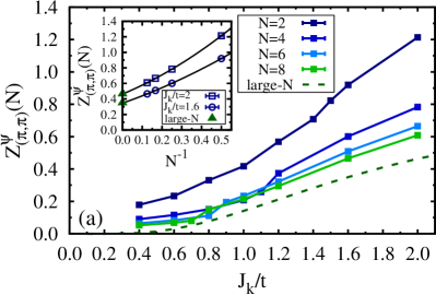
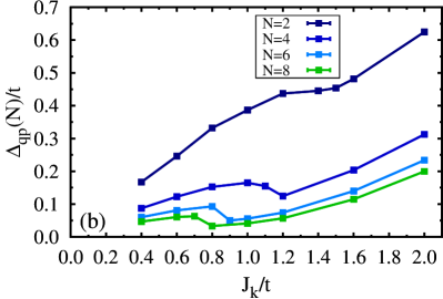
Figure 12: (a) Quasiparticle residue $Z^{\psi}_{(\pi,\pi)}$ and (b) single particle gap $\Delta_{qp}$ of the composite fermion spectral function obtained from $T=0$ QMC simulations of the SU($N$) KLM. For comparison we also show $Z^{\psi}_{(\pi,\pi)}$ predicted by the large-$N$ approximation (dashed line). Inset shows a second-order polynomial fit to the QMC data in order to extract $Z^{\psi}_{(\pi,\pi)}$ in the $N\to\infty$ limit; the extrapolated values $Z^{\psi}_{(\pi,\pi)}(N\to\infty)=0.463(4)$ at $J_{k}/t=2$ and $Z^{\psi}_{(\pi,\pi)}(N\to\infty)=0.345(1)$ at $J_{k}/t=1.6$ match well those obtained using the large-$N$ approximation (triangles).

Next, we look at the evolution of the quasiparticle residue $Z^{\psi}_{(\pi,\pi)}$ as a function of $J_{k}/t$. We summarize it in Fig. 12(a). It conveys the main outcome of our study, i.e., numerical results for $Z^{\psi}_{(\pi,\pi)}$ in the $N=2$ case and in the large-$N$ approach exhibit an entirely different behavior in the small $J_{k}$ limit. This is a counterintuitive result, since, as shown in Eq. (29), the composite fermion operator directly provides the measure of hybridization, ${\hat{\psi}}^{\dagger}_{{\boldsymbol{i}},\sigma}\propto\frac{2}{N}{\hat{f}}^{\dagger}_{{\boldsymbol{i}},\sigma}V$, where $V$ is the hybridization order parameter. Hence, one could expect $A_{\psi}({\boldsymbol{k}},\omega)\propto V^{2}|u_{{\boldsymbol{k}}}|^{2}$, where $|u_{\boldsymbol{k}}|^{2}$ is the coherence factor at the mean-field level, see Eq. (32). However, the spectral weight does not follow the exponentially small Kondo scale, displaying a linear dependency in $J_{k}/t$ instead, in analogy to the linear behavior of the quasiparticle gap, see Fig. 12(b). In the case of the quasiparticle gap, the linear dependency was found to be a direct consequence of particle-hole symmetry and the associated Fermi surface nesting-driven magnetism Martin et al. (2010); Lenz et al. (2017); Eder and Wróbel (2018). The question then arises whether the same holds for the quasiparticle residue $Z^{\psi}_{(\pi,\pi)}$. Given that the influence of the magnetism on $A_{\psi}({\boldsymbol{k}},\omega)$ boils mainly down to the backfolding of the heavy fermion band in the paramagnetic phase, we believe that the observed enhancement of the spectral weight is unrelated to the half-filled conduction band and stems instead from the specific form of the composite fermion operator.

Another notable result is the abrupt reduction of $Z^{\psi}_{(\pi,\pi)}$ across the magnetic order-disorder transition point $J_{c}$ in the highly symmetric case with $N>2$. The ability of $Z^{\psi}_{(\pi,\pi)}$ to reflect the onset of long range magnetic order stems from the sum rule for the composite fermion spectral function Eq. (III.1) which consists of the Kondo term $\langle\hat{\boldsymbol{S}}_{\boldsymbol{i}}\cdot\hat{\boldsymbol{c}}^{\dagger}_{\boldsymbol{i}}\boldsymbol{\sigma}\hat{\boldsymbol{c}}_{\boldsymbol{i}}\rangle$. This quantity was shown in Ref. Raczkowski and Assaad (2020) to display a discontinuous behavior at $J_{c}$ indicating a first-order nature of the transition for $N>2$. The latter is equally seen in the nonmonotonic behavior of the single particle gap, see Fig. 12(b).

Finally, by extrapolating finite-$N$ QMC data at $J_{k}/t=2$ and at $J_{k}/t=1.6$ to the $N\to\infty$ limit, we were able to recover the large-$N$ value of $Z^{\psi}_{(\pi,\pi)}$, see the inset in Fig. 12(a). This confirms that the large-$N$ theory is the correct saddle point of the SU(2) KLM in the Kondo regime.

V.2 Ferromagnetic Kondo lattice

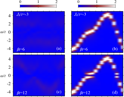
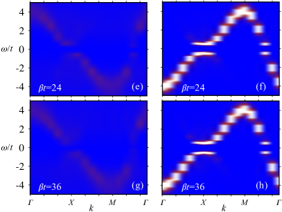
Figure 13: Temperature dependence of $A_{\psi}({\boldsymbol{k}},\omega)$ (left) and $A_{c}({\boldsymbol{k}},\omega)$ (right) in the $12\times 12$ KLM with ferromagnetic coupling $J_{k}/t=-3$: (a,b) $\beta t=6$; (c,d) $\beta t=12$; (e,f) $\beta t=24$, and (g,h) $\beta t=36$.

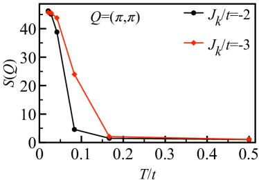
Figure 14: Static spin structure factor $S({\boldsymbol{Q}})$ at ${\boldsymbol{Q}}=(\pi,\pi)$ for the localized spins as a function of temperature $T/t$ in the ferromagnetic KLM.

The ferromagnetic KLM offers the possibility to retain the RKKY interaction and switch off the Kondo effect. Fig. 13 plots the temperature dependence of the composite fermion and conduction electron spectral functions as a function of temperature at $J_{k}/t=-3$. The relevant energy scale required to interpret the plots is the magnetic scale below which antiferromagnetic fluctuations set in. From Fig. 14 we can estimate $T_{RKKY}\simeq 0.125t$. At $T\ll T_{RKKY}$, see Figs. 13(e)-13(h), one finds that the data are well reproduced by the large-$S$ results. In particular the single particle Green’s functions match well the forms:

$$A_{c}({\boldsymbol{k}},\omega)= \frac{1}{2}\left(1+\frac{\epsilon(\boldsymbol{k})}{E(\boldsymbol{k})}\right)\delta(\omega-E(\boldsymbol{k}))+$$ (58)

$$\frac{1}{2}\left(1-\frac{\epsilon(\boldsymbol{k})}{E(\boldsymbol{k})}\right)\delta(\omega+E(\boldsymbol{k})).$$

Here $\epsilon(\boldsymbol{k})=-2t\left(\cos{k_{x}}+\cos{k_{y}}\right)$ is the noninteracting dispersion relation and $E(\boldsymbol{k})=\sqrt{\epsilon(\boldsymbol{k})^{2}+\Delta^{2}}$, with $\Delta$ the gap. Although the dispersion relation is independent of the shift of the ordering wave vector $\boldsymbol{Q}=(\pi,\pi)$, the coherence factors are not. Hence, the dominant weight in $A_{c}({\boldsymbol{k}},\omega)$ [$A_{\psi}({\boldsymbol{k}},\omega)$] follows the noninteracting dispersion relation $\epsilon(\boldsymbol{k})$ [$\epsilon(\boldsymbol{k}+\boldsymbol{Q})$]. This is consistent with the large-$S$ relation of Eq. (III.5) corresponding to $A_{\psi}({\boldsymbol{k}},\omega)\simeq S^{2}A_{c}({\boldsymbol{k}}+\boldsymbol{Q},\omega)$.

At high temperatures, $T>T_{RKKY}$, the magnetically induced gap should vanish and, as argued in Eq. (20), the composite fermion spectral function is expected to show no $\boldsymbol{k}$-dependence. Figures 13(a) and 13(b) confirm the above expectations.

The above demonstrates that the dominant effects of the RKKY interaction can be understood in terms of a large-$S$ or mean-field approximation.

VI Summary and Conclusions

The composite fermion operator we have considered in this article is defined in Eq. (2) and is at best understood in terms of a canonical Schrieffer-Wolff transformation of the electron creation operator in a localized Wannier state of the PAM. We have studied numerically the spectral function of the composite fermion for the SU($N$) antiferromagnetic and SU(2) ferromagnetic KLM on a square lattice and provided a number of insights based on analytical considerations in the large-$N$, large-$S$ and strong coupling limits.

The key result of the paper is numerical. We observe that for the antiferromagnetic SU(2) KLM on the square lattice the spectral function of the composite fermion, $A_{\psi}(\boldsymbol{k},\omega)$, reveals the heavy fermion band and that the spectral weight tracks $J_{k}/t$ in the weak coupling limit. This should be contrasted with the conduction electron spectral function, $A_{c}(\boldsymbol{k},\omega)$, that also captures the heavy fermion band but with spectral weight given by the Kondo scale $e^{-W/J_{k}}$. Hence the composite fermion provides a remarkable enhancement of spectral intensity in the weak coupling limit and greatly facilitates investigations of the heavy fermion band in the realm of the SU(2) KLM.

For model Hamiltonians that support quasiparticle excitations, we generically expect the dispersion relation to be revealed by the spectral function of any operator with appropriate quantum numbers. Thereby, the effective mass of charge carriers – corresponding to the inverse curvature of the dispersion relation – is independent of the choice of the fermion operator. In terms of the self-energy, the effective mass is given by the inverse quasiparticle residue – that stems from its frequency dependency – times a term that reflects its momentum dependence Negele and Orland (1998). Hence $m^{*}=m^{*}_{\boldsymbol{k}}/Z_{\boldsymbol{k}}$. Let us apply the above to the SU(2) KLM. Here $m^{*}\propto e^{W/J_{k}}$ in the weak coupling limit Assaad (2004). Since $Z^{\psi}_{\boldsymbol{k}=(\pi,\pi)}\propto J_{k}$ we conclude that it is the $\boldsymbol{k}$-dependence of the composite fermion self-energy that captures the heavy fermion effective mass. More generally, optimization of the quasiparticle residue necessitates real space fluctuations. Both in the large-$N$ limit Burdin et al. (2000) and at $N=2$ Assaad (2004), the effective mass tracks the inverse Kondo temperature. However, the quasiparticle residue of the composite fermion varies from $Z_{\boldsymbol{k}}\propto e^{-W/J_{k}}$ in the large-$N$ limit to $Z_{\boldsymbol{k}}\propto J_{k}$ at $N=2$ thereby reflecting the buildup of spatial fluctuations as a function of decreasing $N$. Clearly as a function of $N$, and at sufficiently small values of $J_{k}$, we will encounter a magnetic phase transition Raczkowski and Assaad (2020) such that the question arises if the observed enhancement of the spectral weight is a consequence of magnetic fluctuations. We believe that this is not the case since the spectral function of the composite fermion is very well understood in terms of backfolding of the heavy fermion band in the paramagnetic phase and concomitant opening of a single particle gap set by $J_{k}$ reflecting the particle-hole symmetry. Accordingly, the composite fermion opens up the possibility to track the fate of the fragile heavy fermion quasiparticle in the KLM in any situation where competing instabilities lead to a significant suppression of the lattice Kondo effect and thus to extremely low coherence temperatures Raczkowski et al. (2010); Bodensiek et al. (2011); Lechtenberg et al. (2018).

The aforementioned growth of spectral weight between the large-$N$ and SU(2) limits can also be seen when building a KLM by assembling magnetic adatoms on a metallic surface Raczkowski and Assaad (2019). In the single impurity limit the composite fermion local spectral function reveals the Kondo resonance with spectral weight tracking the Kondo scale. As magnetic adatoms are assembled around this initial impurity so as to locally form a half-filled Kondo lattice, the Kondo resonance develops a gap and acquires substantial spectral weight. This is explicitly seen in Fig. 1(c) of Ref. Raczkowski and Assaad (2019).

In the strong coupling limit, the Kondo effect corresponds to the formation of a singlet between the conduction electron and spin degree of freedom in a unit cell. In this limit the half-filled ground state, $|\Psi_{0}^{n}\rangle$, of the SU(2) KLM is a direct product of such singlets. As apparent from Eqs. (III.4) and (III.4), $\hat{c}_{\boldsymbol{i},\uparrow}|\Psi_{0}^{n}\rangle=-2\hat{\psi}_{\boldsymbol{i},\uparrow}|\Psi_{0}^{n}\rangle$. Hence in this limit, we observe, up to a normalization factor, no difference between the $c$- and $\psi$- spectral functions. The strong coupling limit is characterized by fast magnetic fluctuations on the time scale of the motion of a doped electron. Thereby, the picture of a doped hole moving in a Kondo singlet background is appropriate. In the weak coupling limit, magnetic fluctuations are slow in comparison to the hole motion, such that locally the doped hole will perceive a static magnetic background. In this case our results show that $\hat{c}_{\boldsymbol{k},\uparrow}|\Psi_{0}^{n}\rangle$ and $\hat{\psi}_{\boldsymbol{k},\uparrow}|\Psi_{0}^{n}\rangle$ differ substantially. In particular, $\hat{\psi}_{\boldsymbol{k},\uparrow}$ removes a conduction electron and simultaneously adjusts the spin background whereas $\hat{c}_{\boldsymbol{k},\uparrow}$ merely destroys a conduction electron. Our result suggests that $Z^{\psi}_{\boldsymbol{k}=(\pi,\pi)}/Z^{c}_{\boldsymbol{k}=(\pi,\pi)}$ diverges in the weak coupling such that $\hat{\psi}_{\boldsymbol{k},\uparrow}$ captures the correct form of the heavy fermion quasiparticle. In particular it corresponds to a bound state of conduction electron and spin degrees of freedom. The energy scale of the bound state is revealed by $A_{\psi}(\boldsymbol{k},\omega)$, see Fig. 4, as the energy scale above which the quasiparticle pole dissolves into a continuum captured by the convolution of the spin susceptibility and spectral function of the conduction electron. To a first approximation, our results suggest that this energy scale tracks $J_{k}$.

$A_{\psi}(\boldsymbol{k},\omega)$ is a quantity of choice to study Kondo breakdown transitions since at this transition we expect the destruction of the aforementioned bound state. This statement is supported by our large-$N$ results where the composite fermion operator reveals the hybridization matrix element that vanishes at a Kondo breakdown transition. It furthermore follows from the very definition of the composite fermion operator in terms of a Schrieffer-Wolff transformation of the electron creation operator in a localized orbital in the PAM. In particular, in the realm of the PAM and in the Kondo breakdown phase, the localized electrons drop out from the low energy physics. For Kondo breakdown critical points in metallic environments we hence expect $A_{\psi}(\boldsymbol{k},\omega)$ to develop a gap thereby revealing the orbital selective Mott nature of this transition Vojta (2010). This has already been partially observed in Ref. Danu et al. (2020). However, even in an insulating state, Kondo breakdown should correspond to the destruction of the low lying quasiparticle pole in $A_{\psi}(\boldsymbol{k},\omega)$. The fact that we do not observe this for the square lattice, points to the fact that Kondo screening and magnetism coexist down to our lowest considered value of $J_{k}/t=0.4$.

The above can be checked by considering the ferromagnetic Kondo lattice where the Kondo effect is absent. Here, we have seen that the spectral function shows no low lying bound states and that it can be very well understood within a large-$S$ expansion: at leading order in $S$ the composite fermion spectral function reduces to the conduction one shifted by the momentum $\boldsymbol{Q}$ of the magnetic ordering.

The aforementioned derivation of the composite fermion operator from the PAM in the local moment regime, allows us to link our results to experiments. The local composite fermion spectral function can be measured with STM experiments of adatoms on metallic surfaces provided that the current between the STM tip and metallic surface flows through the correlated orbital of the adatom. This has been achieved by capping a metallic surface with an insulating layer on which adatoms reside Toskovic et al. (2016). Photoemission studies of the 4$f$ levels of CePt₅ surface alloys have been presented in Ref. Klein et al. (2008). Since this compound is in the local moment regime, one can conjecture that the appropriate spectral function required to capture the heavy fermion quasiparticle is $A_{\psi}(\boldsymbol{k},\omega)$ in the framework of a Kondo lattice modeling. Our results suggest that the $\boldsymbol{k}$-dependence of the self-energy plays an important role for the understanding of $A_{\psi}(\boldsymbol{k},\omega)$. This may explain why dynamical mean-field calculations in combination with a non-crossing approximation of the spectral function in the realm of the PAM equally presented in Ref. Klein et al. (2008), seem to underestimate the spectral weight of the heavy fermion bands in comparison to experiments.