Probing Geometric Excitations of Fractional Quantum Hall States on Quantum Computers

Abstract

Intermediate-scale quantum technologies provide new opportunities for scientific discovery, yet they also pose the challenge of identifying suitable problems that can take advantage of such devices in spite of their present-day limitations. In solid-state materials, fractional quantum Hall (FQH) phases continue to attract attention as hosts of emergent geometrical excitations analogous to gravitons, resulting from the non-perturbative interactions between the electrons. However, the direct observation of such excitations remains a challenge. Here, we identify a quasi-one-dimensional model that captures the geometric properties and graviton dynamics of FQH states. We then simulate geometric quench and the subsequent graviton dynamics on the IBM quantum computer using an optimally-compiled Trotter circuit with bespoke error mitigation. Moreover, we develop an efficient, optimal-control-based variational quantum algorithm that can efficiently simulate graviton dynamics in larger systems. Our results open a new avenue for studying the emergence of gravitons in a new class of tractable models on the existing quantum hardware.

Introduction. While a universal fault-tolerant quantum computer with thousands of qubits remains elusive, noisy intermediate-scale quantum (NISQ) devices with a few qubits are already operational Arute et al. (2019); Boixo et al. (2018); Neill et al. (2021), albeit with limitations due to a lack of reliable error-correction Wootton (2020). This progress has stirred a flurry of research activity to identify problems that can take advantage of this recently developed quantum technology  Bharti et al. (2021). Utilizing NISQ systems as digitized synthetic platforms to study physics phenomena challenging to investigate otherwise has emerged as a critical frontier Jiang et al. (2018).

In strongly-correlated electron materials, fractional quantum Hall (FQH) states are widely studied for their exotic topological properties, such as excitations with fractional charge Laughlin (1983); de Picciotto et al. (1997) and fractional statistics Nakamura et al. (2020); Bartolomei et al. (2020). Recently, FQH states have come into focus due to their universal geometric features such as Hall viscosity  Avron et al. (1995); Read (2009); Haldane (2009) and the Girvin-MacDonald-Platzman magnetoroton collective mode Girvin et al. (1985, 1986). In the long-wavelength limit $k\to 0$, the magnetoroton forms a quadrupole degree of freedom that carries angular momentum $L=2$ and can be represented by a quantum metric, $\widetilde{g}$ Haldane (2011). For this reason, the $k\to 0$ limit of the magnetoroton has been referred to as “FQH graviton” Yang et al. (2012a); Golkar et al. (2016), due to its formal similarity with the fluctuating space-time metric in a theory of quantum gravity Bergshoeff et al. (2013, 2018).

The experimental detection of the FQH graviton for $\nu=1/3$ Laughlin state remains an outstanding challenge. While at large momenta, $k{\sim}\ell_{B}^{-1}$, with $\ell_{B}=\sqrt{\hbar/eB}$ being the magnetic length, the magnetoroton mode may be probed via inelastic light scattering Pinczuk et al. (1993); Platzman and He (1996); Kang et al. (2001); Kukushkin et al. (2009), the magnetroroton enters the continuum near $k\to 0$ for the $\nu=1/3$ Laughlin state (in contrast to the mode for $\nu=7/3$ Wurstbauer et al. (2015); Jolicoeur (2017)). Haldane proposed that quantum-metric fluctuations can be exposed by breaking rotational symmetry Haldane (2011). Following up on this idea, recent theoretical works Liu et al. (2018); Lapa et al. (2019) have probed the FQH graviton by quenching the metric of “space”, i.e., by suddenly making the FQH state anisotropic (see also alternative proposals Liou et al. (2019); Nguyen and Son (2021); Wang and Yang ). It was found that such geometric quenches induce coherent dynamics of the FQH graviton Liu et al. (2018), even though the graviton mode resides at finite energy densities above the FQH ground state. In contrast, near the FQH liquid-nematic phase transition Xia et al. (2011); Samkharadze et al. (2016), the graviton is expected to emerge as a gapless excitation Regnault et al. (2017); You et al. (2014); Yang (2020).

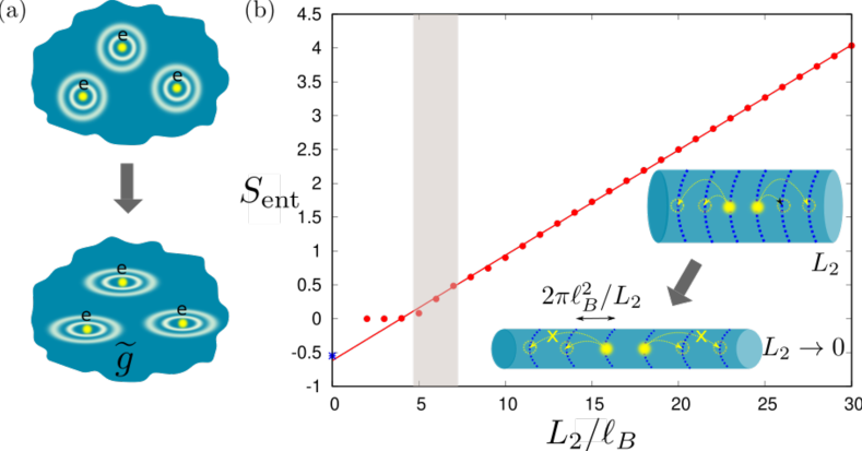
Figure 1: (a) Geometric quench probes the fluctuations of the quantum metric $\widetilde{g}$ Haldane (2011). (b) Entanglement entropy $S_{\mathrm{ent}}$ for the $\nu{=}1/3$ Laughlin state on a cylinder as a function of the circumference $L_{2}$. Entropy obeys the area law for sufficiently large circumferences $L_{2}\gtrsim 5\ell_{B}$, with a subleading correction close to the expected value $-\ln(3)/2$ (blue star). Data is obtained using the matrix product method Zaletel and Mong (2012); Estienne et al. (2013) with entanglement truncation $P_{\mathrm{max}}{=}18$. Near the thin-cylinder limit (shaded), long-range electron hopping becomes strongly suppressed, as shown in the inset.

In this paper, we realize the FQH graviton in a synthetic NISQ system – the IBM open-access digitized quantum processor – and simulate its out-of-equilibrium dynamics. We first map the problem onto a one-dimensional quantum spin chain, corresponding to the FQH state on a thin cylinder. While topological properties of FQH states have been extensively studied in this regime Rezayi and Haldane (1994); Bergholtz and Karlhede (2005); Seidel et al. (2005); Bergholtz and Karlhede (2008); Rahmani et al. (2020); Nakamura et al. (2012); Wang and Nakamura (2013); Soulé and Jolicoeur (2012), we show that this limit remarkably captures some geometric properties of FQH systems, in particular their quench dynamics. As a second step, we implement the quench dynamics on the IBM NISQ device, using two complementary approaches. On the one hand, we used an optimally-compiled, noise-aware Trotterization circuit with error mitigation methods Saravanan and Saeed (2022); Abraham and et al. (2019); Davis et al. (2020). This allowed us to successfully simulate quench dynamics on the IBM device, overcoming the problem of the large circuit depth. On the other hand, we devised an efficient optimal-control-based Werschnik and Gross (2007); Petersen and Dong (2010); Rahmani (2013) variational quantum algorithm Peruzzo et al. (2014); Wecker et al. (2015, 2016); McClean et al. (2016), analogous to the Quantum Approximate Optimization Algorithm (QAOA) Farhi et al. ; Farhi and Harrow ; Yang et al. (2017); Wang et al. (2018); Zhou et al. (2020); Lin et al. (2021), that creates the post-quench state using a hybrid classical-quantum approach Kokail et al. (2019); Kandala et al. (2017). We demonstrate that this method scales favorably with system size, with a linear-depth circuit depth and only two variational parameters.

Anisotropic Laughlin state near the thin-cylinder limit. We focus on the $\nu{=}1/3$ Laughlin FQH state Laughlin (1983) whose Hamiltonian near the thin-cylinder (TC) limit is given by Nakamura et al. (2012)

$$\hat{H} =\sum_{j}V_{1,0}\hat{n}_{j}\hat{n}_{j+1}+V_{2,0}\hat{n}_{j}\hat{n}_{j+2}+V_{3,0}\hat{n}_{j}\hat{n}_{j+3}$$ (1)

$$+V_{2,1}c^{\dagger}_{j+1}c^{\dagger}_{j+2}c_{j+3}c_{j}+\mathrm{h.c.}$$

Here the operators $c_{j}$, $c_{j}^{\dagger}$ ($\hat{n}_{j}{\equiv}c_{j}^{\dagger}c_{j}$) destroy or create an electron in a Landau level (LL) orbital localized around $2\pi j\ell_{B}^{2}/L_{2}$. We assume the system is defined on a cylinder of size $L_{1}{\times}L_{2}$ containing $N$ electrons, such that the filling factor $\nu{=}N/N_{\phi}{=}1/3$, with magnetic flux $N_{\phi}{=}(L_{1}L_{2})/(2\pi\ell_{B}^{2})$. The near-TC limit corresponds to $L_{1}{\gg}L_{2}$ with the area ($N_{\phi}$) fixed, which allows us to neglect longer-range interaction terms beyond those in Eq. (1). Importantly, the Hamiltonian above describes a 2D system with strong spatial anisotropy, as opposed to a strictly 1D limit $L_{2}{\to}0$, thus allowing the emergence of the graviton mode. The interaction matrix elements are given by

$$V_{k,m}=(k^{2}-m^{2})e^{-2\pi^{2}(k^{2}+m^{2}-2ikmg_{12})/{L_{2}^{2}g_{11}}},$$ (2)

which we have generalized to the case of an arbitrary electron mass tensor $g_{ab}$, $a,b=1,2$. The mass tensor must be symmetric and unimodular ($\mathrm{det}g{=}1$) Haldane (2011), hence we can generally write it as $g=\exp(\hat{Q})$ where $\hat{Q}=Q(2\hat{d}_{a}\hat{d}_{b}-\delta_{a,b})$ is a Landau-de Gennes order parameter and $\hat{\mathbf{d}}=(\cos(\phi/2),\sin(\phi/2))$ is a unit vector Maciejko et al. (2013). Parameters $Q$ and $\phi$ intuitively represent the stretch and rotation of the metric, respectively. The FQH state is invariant under area-preserving deformations of $g$, illustrated in Fig. 1(a).

Since the Hamiltonian in Eq. (1) is positive semi-definite, it has a unique (unnormalized) ground state with zero energy Nakamura et al. (2012)

$$|\psi_{0}\rangle=\prod_{j}\left(1-\sqrt{\frac{V_{3,0}}{V_{1,0}}}e^{i\frac{8\pi^{2}\ell_{B}^{2}}{L_{2}^{2}}\frac{g_{12}}{g_{11}}}\hat{S}_{j}\right)|\ldots 100100\ldots\rangle,\;\;\;\;$$ (3)

where $\hat{S}_{j}{=}c_{j+1}^{\dagger}c_{j+2}^{\dagger}c_{j+3}c_{j}$ is an operator that “squeezes” two neighbouring electrons while preserving their center-of-mass position Bernevig and Haldane (2008). The ground state in the limit $L_{2}{\to}0$ is the product state $|...100100...\rangle$. The off-diagonal squeezing operator is essential for the $1/3$ Laughlin state Rezayi and Haldane (1994).

In previous works Rezayi and Haldane (1994); Nakamura et al. (2012); Wang and Nakamura (2013); Soulé and Jolicoeur (2012), the ground state of the model in Eq. (1) and its neutral excitations were studied on isotropic cylinders, $g_{11}{=}g_{22}{=}1$, $g_{12}{=}0$. In particular, it was found that the state in Eq. (3) has ${\sim}98\%$ overlap with the ground state of the full Hamiltonian in the range of circumferences $5\ell_{B}\lesssim L_{2}\lesssim 7\ell_{B}$, where $V_{2,1}/V_{1,0}\approx 0.2-0.3$, justifying the use of the truncated model Eq. (1) in this regime Nakamura et al. (2012). We have confirmed that the same conclusions continue to hold in the presence of mass anisotropy SOM (2021).

As a further justification of the model in Eq. (1), we plot the entanglement entropy $S_{\mathrm{ent}}$ of the Laughlin state in a large system of 100 electrons as a function of the circumference $L_{2}$ in Fig. 1(b). We see that it is possible to reduce $L_{2}$ to approximately $5\ell_{B}$, where the “area law” for entanglement entropy Kitaev and Preskill (2006); Levin and Wen (2006) still holds, but long-range electron hopping is strongly suppressed. Below we focus on this regime, where the key aspects of 2D physics are preserved, but the system can be mapped to a 1D spin chain model and thus efficiently simulated on quantum hardware.

Geometric quench. We now show that, in addition to the ground state, the effective model in Eq. (1) captures the high-energy excitations that govern the graviton dynamics in the FQH phase. We initially prepare the system in the ground state $|\psi_{0}\rangle$ in Eq. (3) with isotropic metric ($g_{11}{=}g_{22}{=}1$, $g_{12}{=}0$). At time $t{=}0$, we instantaneously introduce diagonal anisotropy, $g_{11}^{\prime}{=}1/g_{22}^{\prime}{>}1$, and let the system evolve unitarily, under the dynamics generated by the post-quench anisotropic Hamiltonian. We are interested in the dynamical fluctuations of its quantum metric $\widetilde{g}$ as the system is taken out of equilibrium.

Note, even though $g$ and $\widetilde{g}$ are related to one another, $\widetilde{g}$ is an emergent property of a many-body state and not necessarily equal to $g$. Nevertheless, we can formally parameterize $\widetilde{g}$ using the parameters $\widetilde{Q}$ and $\widetilde{\phi}$, representing the stretch and rotation of the emergent metric. In order to determine the equations of motion for $\widetilde{Q}$ and $\widetilde{\phi}$, we maximize the overlap between $|\psi(t)\rangle$ and the family of trial states in Eq. (3) Yang et al. (2012b). When this overlap is close to unity, we can be confident that we found the optimal metric parameters $\widetilde{Q}$ and $\widetilde{\phi}$ describing the state $|\psi(t)\rangle$.

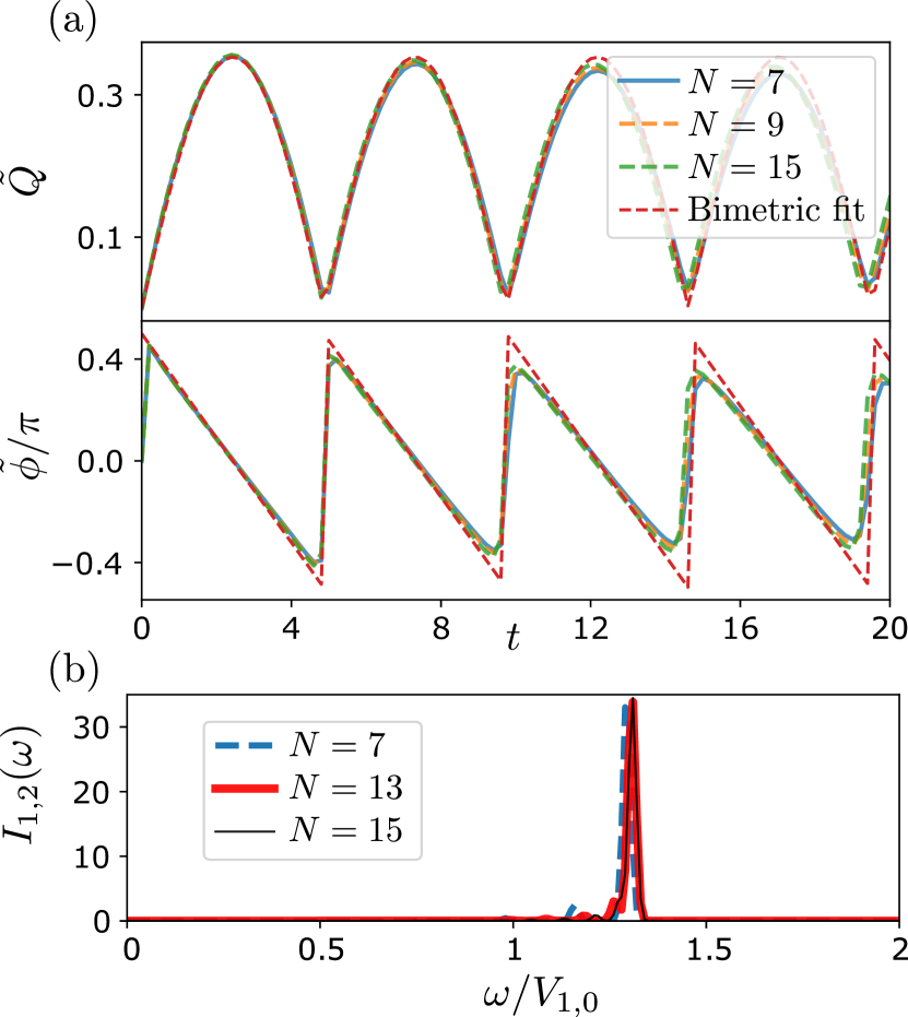
Figure 2: (a) Dynamics of $\widetilde{Q}$ and $\widetilde{\phi}$ following the geometric quench in the TC limit, with $L_{2}{=}5.477\ell_{B}$ and post-quench anisotropy $Q{\approx}0.18$. Data is for system sizes $N{=}7,9,15$ electrons. (b) Quadrupole spectral function, $I_{1,2}$, shows a sharp peak at the graviton energy $E_{g}{\approx}1.29$, which agrees well with the frequency of the oscillations in (a).

In Fig. 2, we summarize the results of the graviton dynamics in the model in Eq. (1) when anisotropy is suddenly changed from $Q{=}0$ to $Q{\approx}0.18$ while keeping $\phi{=}0$. Fig. 2(a) shows the dynamics of $\widetilde{Q}$ and $\widetilde{\phi}$ for different system sizes $N$. The dynamics is in excellent agreement with the bimetric theory in the linear regime Gromov and Son (2017),

$$\widetilde{Q}(t)=\pm 2A\sin\frac{E_{g}t}{2},\quad\widetilde{\phi}(t)=\pm\frac{\pi}{2}-\frac{E_{g}t}{2},$$ (4)

where $E_{g}$ is the energy of the graviton mode in units of $V_{1,0}$. As can be seen in Fig. 2(a), the numerical data can be accurately fitted using Eqs. (4). The fit yields the oscillation frequency $E_{g}{=}1.29$. Note that this energy is much higher than the first excited energy of the quench Hamiltonian. We identify this energy with the graviton state as evidenced by the sharp peak in the quadrupole ($L=2$) spectral function $I_{1,2}(\omega)$ Yang (2016). The later spectral function is designed to detect the characteristic $d-$wave symmetry of the graviton. Analogous to an oscillating space-time metric induced by a gravitational wave, $I_{1,2}(\omega)$ is the associated transition rate due to the dynamics of the oscillating mass-tensor Yang (2016). Thus, the model in Eq. (1) reproduces the graviton oscillation as described by the bimetric theory.

Spin chain mapping. We use the reduced registers scheme introduced in Ref. Rahmani et al. (2020) to map the model (1) to a spin chain, see also SOM (2021) for further details. The reduced register is a block of three consecutive orbitals that encodes whether or not the block is “squeezed” with respect to the root state $|100,100,\dots\rangle$. For each block of three sites, the state of the reduced register is $\mathbb{1}$ if it is squeezed (i.e., $011$) or $\mathbb{0}$ if not (i.e., either $000$ or $100$). In the root state, none of the blocks are squeezed and it maps to $|{\mathbb{0}},{\mathbb{0}},{\mathbb{0}},\dots\rangle$. If we apply the squeezing operator to one block of the root state, we obtain, e.g., $|100,011,000,\dots\rangle\to|{\mathbb{0}},{\mathbb{1}},{\mathbb{0}},\dots\rangle$. In terms of reduced registers, squeezing acts as flip of $\mathbb{0}$ to $\mathbb{1}$, so it can be viewed as the Pauli $X$ matrix. However, there is an important difference in that the Hilbert space is not a tensor product of reduced registers, since the squeezing can never generate two neighboring $\ldots\mathbb{1}\mathbb{1}\ldots$ configurations of the reduced registers Moudgalya et al. (2020, 2019). This type of constrained Hilbert space arises e.g., in the Fibonacci anyon chain Feiguin et al. (2007). The inverse mapping is constructed as follows: for any $\mathbb{1}$ we make a $011$ block. A $\mathbb{0}$ that follows a $\mathbb{1}$ ($\mathbb{0}$) gives a $000$ ($100$) block. With this mapping of states, we can show that the Hamiltonian (1) maps to a local spin-chain Hamiltonian

$$\begin{split}\hat{H}=&\sum_{\ell}\left((V_{1,0}-3V_{3,0}){\cal N}_{\ell}+V_{3,0}{\cal N}_{\ell}{\cal N}_{\ell+2}\right.\\ &\left.+(1-{\cal N}_{\ell-1})[{\rm Re}(V_{2,1})X_{\ell}-{\rm Im}(V_{2,1})Y_{\ell}](1-{\cal N}_{\ell+1})\right),\end{split}$$ (5)

where we omitted the boundary terms for simplicity and introduced the occupation number $\cal N{\equiv}|\mathbb{1}\rangle\langle\mathbb{1}|$, Pauli $X{\equiv}|\mathbb{0}\rangle\langle\mathbb{1}|{+}|\mathbb{1}\rangle\langle\mathbb{0}|$, and Pauli $Y{\equiv}-i|\mathbb{0}\rangle\langle\mathbb{1}|{+}i|\mathbb{1}\rangle\langle\mathbb{0}|$ operators.

Figure 3: Circuit implementation of the trotterized unitary $U_{\ell}$ in the bulk of the spin chain.

Quantum simulation. The standard procedure for simulating the time evolution $e^{-i\hat{H}t}$ is to use Trotter decomposition. Here $\hat{H}$ is given in equation Eq. (5) with real $V_{2,1}$ and it has the form $\hat{H}=\sum_{\ell}H_{\ell}$. We decompose the evolution operator into $k$ Trotter steps as $e^{-i\hat{H}t}\approx\left[\prod_{l}U_{\ell}(t/k)\right]^{k}$, where $\delta t=t/k$ and the approximation improves for larger $k$. In SOM (2021) we derive the circuit which implements a Trotterized time evolution of our Hamiltonian and the subcircuit for the bulk $U_{\ell}(\delta t)$ is shown in Fig. 3. Below we demonstrate this circuit yields good results on current IBM devices with 5 qubits after using noise-aware error mitigation methods and optimized compilations Saravanan and Saeed (2022); Abraham and et al. (2019); Davis et al. (2020).

While the trotterization algorithm emulates the actual quantum evolution resulting from FQH quenched Hamiltonian, it has a relatively large number of entangling gates. We can access large systems by a hybrid classical-quantum method that requires classical optimization, using the following variational ansatz for the final post-quench state $|\psi(t)\rangle$:

$$|\psi_{\rm var}(\alpha,\beta)\rangle=\prod_{\ell}e^{-i\alpha{\cal N}_{\ell}}e^{-i\beta(1-{\cal N}_{\ell-1})X_{\ell}}|\mathbb{000}\dots\rangle,\quad$$ (6)

where on each reduced register $\ell$, we apply alternating gates ${\cal N}_{\ell}$ and $(1-{\cal N}_{\ell-1})X_{\ell}$ (on the very first site, due to open boundary condition, we use $X_{1}$ instead of $(1-{\cal N}_{\ell-1})X_{\ell}$ for $\ell{=}1$).

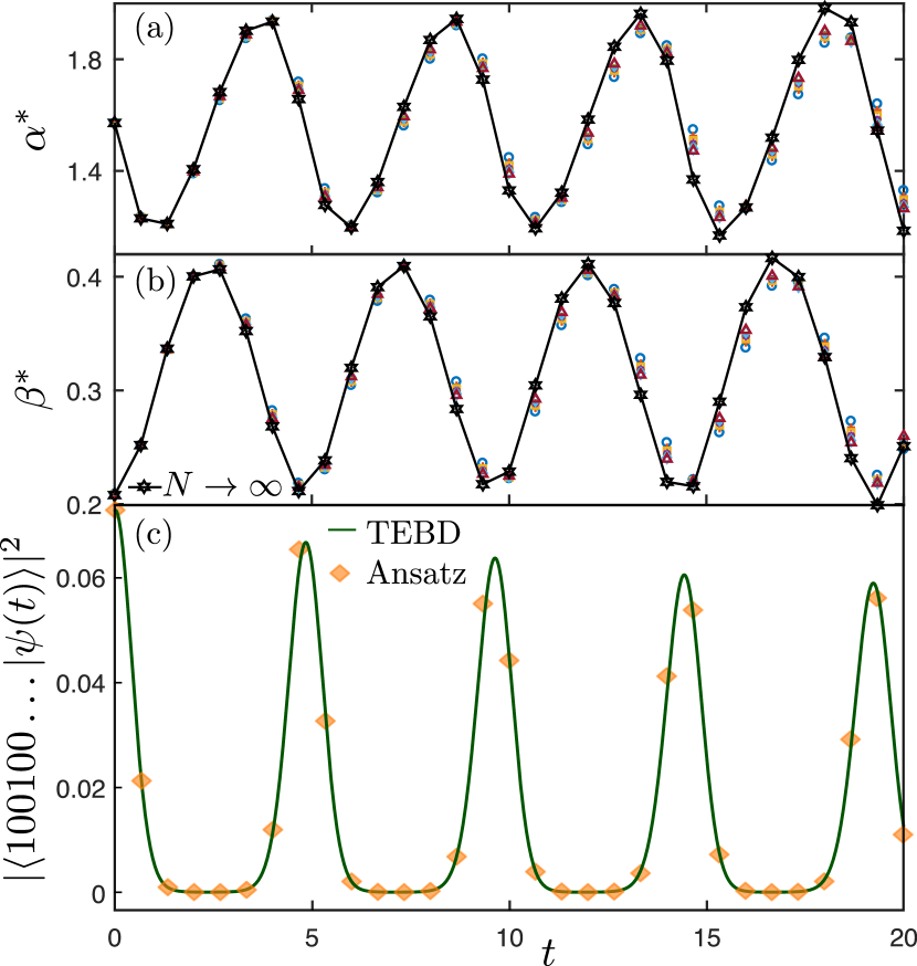
Figure 4: (a)-(b): Optimal variational parameters $\alpha^{*}$ and $\beta^{*}$ for $N=7{-}13$ particles and their extrapolation to $N{\to}\infty$ (solid black line). Optimal parameters vary smoothly with time and exhibit weak finite-size effects. (c) Comparison of the variational ansatz against TEBD simulation for $N{=}60$ for the overlap of the time evolved state with the root state. The parameters of the variational ansatz are extrapolated to the same system size, $N{=}60$. The ansatz with extrapolated parameters exhibits excellent agreement with the TEBD results. TEBD simulations were performed using a bond dimension 20 with a time step $\Delta t{=}0.01$, resulting in truncation error $10^{-5}$.

The optimal parameters $\alpha^{*},\beta^{*}\in[0,2\pi)$ are determined at each time step $t$ using classical optimization by the dual annealing algorithm to maximize the overlap, $|\langle\psi_{0}|U^{\dagger}(t)|\psi_{\rm var}(\alpha,\beta)\rangle|$, with the exact state. Naively, it appears that the classical optimization needs to be performed for each $t$ and system size. Importantly, however, we find the optimal parameters $\alpha^{*}$, $\beta^{*}$ to exhibit a simple oscillatory behavior as a function of time, as well as weak dependence on the system size as shown in Fig. 4(a)-(b). The data for system sizes $N=7,\dots,13$ almost collapse, allowing a smooth extrapolation to the thermodynamic limit ($N{\to}\infty$), shown as the solid black line. In Fig. 4(c), we have checked using time-evolved block decimation (TEBD) Vidal (2004) that the extrapolated parameters produce excellent agreement with direct TEBD calculation of $|\psi(t)\rangle$ for larger systems. Thus, the weak system-size dependence of the variational parameters eliminates the need to directly perform the classical optimization for the actual size of the system, providing access to system sizes for which the classical optimization is infeasible.

Our variational algorithm’s circuit depth scales as the number of qubits $N$ independent of the evolution time $t$. As for trotterization, since we have a local lattice model in one dimension with no explicit Hamiltonian time dependence, the total circuit depth is expected to scale as $Nt$ for a fixed error tolerance Haah et al. ; Childs et al. (2021). Despite higher complexity, trotterization corresponds to the actual unitary operator describing the quantum evolution and does not need any classical optimization or variational ansatz. Both algorithms have good scalability potential to more qubits.

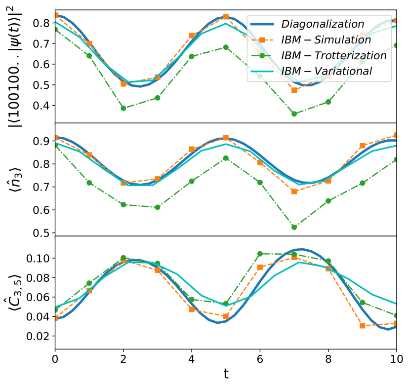
Figure 5: $N=5$ quench results for the time dependence of fidelity, density and correlation function. Comparison between exact diagonalization results, $k=15$ depth Trotterization circuit on the IBM simulator, gate optimized unitary output from IBM-Perth and variational ansatz results from IBM-Santiago. The dynamics have been simulated on IBM-Perth on date: JAN-07-2022 and on IBM-Santiago on JUN-12-2021.

Results on the IBM Quantum Processor. In Fig. 5, we present our measurements of the root state fidelity $|\langle\psi(t))|100100...\ldots\rangle|^{2}$, the local density $\langle n_{j}\rangle$ and the equal-time density-density correlation function $C_{i,j}(t)=-\langle n_{i}(t)n_{j}(t)\rangle+\langle n_{i}(t)\rangle\langle n_{j}(t)\rangle$. While these quantities are in terms of the original fermionic basis, they are easily extracted from measurements in the reduced basis using the rules discussed above Eq. (5). As shown in Fig. 5, the variational results are in excellent agreement the simulations. Similarly, the error-mitigated Trotter algorithm faithfully generates oscillations with the expected graviton frequency despite deeper circuits and higher execution-time error rates than the variational algorithm, which only induce quantitative shifts.

We note that the noise levels of the IBM devices vary widely. Using qiskit library, we executed error-mitigated circuit for the trottrization algorithm on ibmq_perth processor IBM (2021) with readout error, CNOT noise and T2 dephasing time of roughly $1.4$%, $1.7$% and $109$ $\mu$s respectively. The variational ansatz was executed on IBM’s ibmq_santiago processor IBM (2021) with averaged readout error, CNOT noise and T2 dephasing time of roughly $1.5$%, $0.6$% and $120$ $\mu$s, respectively. We also performed simulations of our circuits in qiskit for comparison. Using post-selection methods, we improve the measurements by discarding states that lie outside the physical Hilbert space.

Conclusions. We showed that quantum-geometrical features of FQH states can be realized in an effective 1D model that has an efficient quantum-circuit representation. Our 1D model makes efficient use of resources, as each qubit corresponds to three Landau orbitals, reminiscent of holographic quantum simulation Foss-Feig et al. (2020). As a proof of principle, utilizing the quantum-circuit mapping, we developed efficient quantum algorithms that allowed us to simulate graviton dynamics on IBM quantum processors. We used state-of-the-art error mitigation to successfully run the deep trotterization circuit, which does not require any classical optimization. We also developed a variational algorithm with a linear circuit depth (independent of the evolution time), which makes use of classical optimization but can be scaled to the thermodynamic limit. We expect these results will motivate further analytical investigations into tractable models of graviton dynamics in condensed matter systems, as well as their realizations on NISQ devices.

I Acknowledgements

We thank Areg Ghazaryan and Zhao Liu for useful comments. We acknowledge the use of IBM Quantum services for this work. The views expressed are those of the authors, and do not reflect the official policy or position of IBM or the IBM Quantum team. A.K. is supported by grant numbers DMR-2037996 and DMR-2038028. P.G. acknowledges support from NSF award number DMR-2037996 and DMR-1824265. A.R. acknowledges support from NSF Awards DMR-1945395 and DMR-2038028. A.R. and Z.P. thank the Kavli Institute for Theoretical Physics, acknowledging support by the NSF under Grant PHY1748958. Z.P. and K.B. acknowledge support by EPSRC Grants No. EP/R020612/ 1 and and No. EP/M50807X/1, and by the Leverhulme Trust Research Leadership Award No. RL-2019-015. Statement of compliance with EPSRC policy framework on research data: This publication is theoretical work that does not require supporting research data.

References

- Arute et al. (2019) F. Arute et al., Nature 574, 505 (2019).
- Boixo et al. (2018) S. Boixo, S. V. Isakov, V. N. Smelyanskiy, R. Babbush, N. Ding, Z. Jiang, M. J. Bremner, J. M. Martinis, and H. Neven, Nature Physics 14, 595 (2018).
- Neill et al. (2021) C. Neill et al., Nature 594, 508 (2021).
- Wootton (2020) J. R. Wootton, Quantum Science and Technology 5, 044004 (2020).
- Bharti et al. (2021) K. Bharti et al., “Noisy intermediate-scale quantum (nisq) algorithms,” (2021), arXiv:2101.08448 [quant-ph] .
- Jiang et al. (2018) Z. Jiang, K. J. Sung, K. Kechedzhi, V. N. Smelyanskiy, and S. Boixo, Phys. Rev. Applied 9, 044036 (2018).
- Laughlin (1983) R. B. Laughlin, Phys. Rev. Lett. 50, 1395 (1983).
- de Picciotto et al. (1997) R. de Picciotto, M. Reznikov, M. Heiblum, V. Umansky, G. Bunin, and D. Mahalu, Nature 389, 162 (1997).
- Nakamura et al. (2020) J. Nakamura, S. Liang, G. C. Gardner, and M. J. Manfra, Nature Physics 16, 931 (2020).
- Bartolomei et al. (2020) H. Bartolomei, M. Kumar, R. Bisognin, A. Marguerite, J.-M. Berroir, E. Bocquillon, B. Plaçais, A. Cavanna, Q. Dong, U. Gennser, Y. Jin, and G. Fève, Science 368, 173 (2020).
- Avron et al. (1995) J. E. Avron, R. Seiler, and P. G. Zograf, Phys. Rev. Lett. 75, 697 (1995).
- Read (2009) N. Read, Phys. Rev. B 79, 045308 (2009).
- Haldane (2009) F. D. M. Haldane, ArXiv e-prints (2009), arXiv:0906.1854 [cond-mat.str-el] .
- Girvin et al. (1985) S. M. Girvin, A. H. MacDonald, and P. M. Platzman, Phys. Rev. Lett. 54, 581 (1985).
- Girvin et al. (1986) S. M. Girvin, A. H. MacDonald, and P. M. Platzman, Phys. Rev. B 33, 2481 (1986).
- Haldane (2011) F. D. M. Haldane, Phys. Rev. Lett. 107, 116801 (2011).
- Yang et al. (2012a) B. Yang, Z.-X. Hu, Z. Papić, and F. D. M. Haldane, Phys. Rev. Lett. 108, 256807 (2012a).
- Golkar et al. (2016) S. Golkar, D. X. Nguyen, and D. T. Son, Journal of High Energy Physics 2016, 21 (2016).
- Bergshoeff et al. (2013) E. A. Bergshoeff, S. de Haan, O. Hohm, W. Merbis, and P. K. Townsend, Phys. Rev. Lett. 111, 111102 (2013).
- Bergshoeff et al. (2018) E. A. Bergshoeff, J. Rosseel, and P. K. Townsend, Physical review letters 120, 141601 (2018).
- Pinczuk et al. (1993) A. Pinczuk, B. S. Dennis, L. N. Pfeiffer, and K. West, Phys. Rev. Lett. 70, 3983 (1993).
- Platzman and He (1996) P. M. Platzman and S. He, Phys. Scr. T66, 167 (1996).
- Kang et al. (2001) M. Kang, A. Pinczuk, B. S. Dennis, L. N. Pfeiffer, and K. W. West, Phys. Rev. Lett. 86, 2637 (2001).
- Kukushkin et al. (2009) I. V. Kukushkin, J. H. Smet, V. W. Scarola, V. Umansky, and K. von Klitzing, Science 324, 1044 (2009).
- Wurstbauer et al. (2015) U. Wurstbauer, A. L. Levy, A. Pinczuk, K. W. West, L. N. Pfeiffer, M. J. Manfra, G. C. Gardner, and J. D. Watson, Phys. Rev. B 92, 241407 (2015).
- Jolicoeur (2017) T. Jolicoeur, Phys. Rev. B 95, 075201 (2017).
- Liu et al. (2018) Z. Liu, A. Gromov, and Z. Papić, Phys. Rev. B 98, 155140 (2018).
- Lapa et al. (2019) M. F. Lapa, A. Gromov, and T. L. Hughes, Phys. Rev. B 99, 075115 (2019).
- Liou et al. (2019) S.-F. Liou, F. D. M. Haldane, K. Yang, and E. H. Rezayi, Phys. Rev. Lett. 123, 146801 (2019).
- Nguyen and Son (2021) D. X. Nguyen and D. T. Son, Phys. Rev. Research 3, 023040 (2021).
- (31) Y. Wang and B. Yang, “Analytic exposition of the graviton modes in fractional quantum hall effects and its physical implications,” arXiv:arXiv:2109.08816 .
- Xia et al. (2011) J. Xia, J. P. Eisenstein, L. N. Pfeiffer, and K. W. West, Nature Physics 7, 845 (2011).
- Samkharadze et al. (2016) N. Samkharadze, K. A. Schreiber, G. C. Gardner, M. J. Manfra, E. Fradkin, and G. A. Csáthy, Nature Physics 12, 191 (2016).
- Regnault et al. (2017) N. Regnault, J. Maciejko, S. A. Kivelson, and S. L. Sondhi, Phys. Rev. B 96, 035150 (2017).
- You et al. (2014) Y. You, G. Y. Cho, and E. Fradkin, Phys. Rev. X 4, 041050 (2014).
- Yang (2020) B. Yang, Phys. Rev. Research 2, 033362 (2020).
- Zaletel and Mong (2012) M. P. Zaletel and R. S. K. Mong, Phys. Rev. B 86, 245305 (2012).
- Estienne et al. (2013) B. Estienne, Z. Papić, N. Regnault, and B. A. Bernevig, Phys. Rev. B 87, 161112 (2013).
- Rezayi and Haldane (1994) E. H. Rezayi and F. D. M. Haldane, Phys. Rev. B 50, 17199 (1994).
- Bergholtz and Karlhede (2005) E. J. Bergholtz and A. Karlhede, Phys. Rev. Lett. 94, 026802 (2005).
- Seidel et al. (2005) A. Seidel, H. Fu, D.-H. Lee, J. M. Leinaas, and J. Moore, Phys. Rev. Lett. 95, 266405 (2005).
- Bergholtz and Karlhede (2008) E. J. Bergholtz and A. Karlhede, Phys. Rev. B 77, 155308 (2008).
- Rahmani et al. (2020) A. Rahmani, K. J. Sung, H. Putterman, P. Roushan, P. Ghaemi, and Z. Jiang, PRX Quantum 1, 020309 (2020).
- Nakamura et al. (2012) M. Nakamura, Z.-Y. Wang, and E. J. Bergholtz, Phys. Rev. Lett. 109, 016401 (2012).
- Wang and Nakamura (2013) Z.-Y. Wang and M. Nakamura, Phys. Rev. B 87, 245119 (2013).
- Soulé and Jolicoeur (2012) P. Soulé and T. Jolicoeur, Phys. Rev. B 85, 155116 (2012).
- Saravanan and Saeed (2022) V. Saravanan and S. M. Saeed, “Pauli error propagation-based gate reschedulingfor quantum circuit error mitigation,” (2022), arXiv:2201.12946 [quant-ph] .
- Abraham and et al. (2019) H. Abraham and et al., “Qiskit: An open-source framework for quantum computing,” (2019).
- Davis et al. (2020) M. G. Davis, E. Smith, A. Tudor, K. Sen, I. Siddiqi, and C. Iancu, in 2020 IEEE International Conference on Quantum Computing and Engineering (QCE) (2020) pp. 223–234.
- Werschnik and Gross (2007) J. Werschnik and E. K. U. Gross, arXiv:0707.1883 (2007).
- Petersen and Dong (2010) I. Petersen and D. Dong, IET Control Theory & Applications 4, 2651 (2010).
- Rahmani (2013) A. Rahmani, Mod. Phys. Lett. B 27, 1330019 (2013).
- Peruzzo et al. (2014) A. Peruzzo, J. McClean, P. Shadbolt, M. H. Yung, X. Q. Zhou, P. J. Love, A. Aspuru-Guzik, and J. L. O’Brien, Nat. Comm. 5, 4213 (2014).
- Wecker et al. (2015) D. Wecker, M. B. Hastings, and M. Troyer, Phys. Rev. A 92, 042303 (2015).
- Wecker et al. (2016) D. Wecker, M. B. Hastings, and M. Troyer, Phys. Rev. A 94, 022309 (2016).
- McClean et al. (2016) J. R. McClean, J. Romero, R. Babbush, and A. Aspuru-Guzik, New Journal of Physics 18, 023023 (2016).
- (57) E. Farhi, J. Goldstone, and S. Gutmann, “A Quantum Approximate Optimization Algorithm,” arXiv:1411.4028 .
- (58) E. Farhi and A. W. Harrow, “Quantum supremacy through the quantum approximate optimization algorithm,” arXiv:1602.07674 .
- Yang et al. (2017) Z.-C. Yang, A. Rahmani, A. Shabani, H. Neven, and C. Chamon, Phys. Rev. X 7, 021027 (2017).
- Wang et al. (2018) Z. Wang, S. Hadfield, Z. Jiang, and E. G. Rieffel, Phys. Rev. A 97, 022304 (2018).
- Zhou et al. (2020) L. Zhou, S.-T. Wang, S. Choi, H. Pichler, and M. D. Lukin, Phys. Rev. X 10, 021067 (2020).
- Lin et al. (2021) S.-H. Lin, R. Dilip, A. G. Green, A. Smith, and F. Pollmann, PRX Quantum 2, 010342 (2021).
- Kokail et al. (2019) C. Kokail, C. Maier, R. van Bijnen, T. Brydges, M. K. Joshi, P. Jurcevic, C. A. Muschik, P. Silvi, R. Blatt, C. F. Roos, and P. Zoller, Nature 569, 355 (2019).
- Kandala et al. (2017) A. Kandala, A. Mezzacapo, K. Temme, M. Takita, M. Brink, J. M. Chow, and J. M. Gambetta, Nature 549, 242 (2017).
- Maciejko et al. (2013) J. Maciejko, B. Hsu, S. A. Kivelson, Y. Park, and S. L. Sondhi, Phys. Rev. B 88, 125137 (2013).
- Bernevig and Haldane (2008) B. A. Bernevig and F. D. M. Haldane, Phys. Rev. Lett. 100, 246802 (2008).
- SOM (2021) “Supplemental online material,” (2021).
- Kitaev and Preskill (2006) A. Kitaev and J. Preskill, Phys. Rev. Lett. 96, 110404 (2006).
- Levin and Wen (2006) M. Levin and X.-G. Wen, Phys. Rev. Lett. 96, 110405 (2006).
- Yang et al. (2012b) B. Yang, Z. Papić, E. H. Rezayi, R. N. Bhatt, and F. D. M. Haldane, Phys. Rev. B 85, 165318 (2012b).
- Gromov and Son (2017) A. Gromov and D. T. Son, Phys. Rev. X 7, 041032 (2017).
- Yang (2016) K. Yang, Phys. Rev. B 93, 161302 (2016).
- Moudgalya et al. (2020) S. Moudgalya, B. A. Bernevig, and N. Regnault, Phys. Rev. B 102, 195150 (2020).
- Moudgalya et al. (2019) S. Moudgalya, A. Prem, R. Nandkishore, N. Regnault, and B. A. Bernevig, “Thermalization and its absence within krylov subspaces of a constrained hamiltonian,” (2019), arXiv:1910.14048 [cond-mat.str-el] .
- Feiguin et al. (2007) A. Feiguin, S. Trebst, A. W. W. Ludwig, M. Troyer, A. Kitaev, Z. Wang, and M. H. Freedman, Phys. Rev. Lett. 98, 160409 (2007).
- Vidal (2004) G. Vidal, Phys. Rev. Lett. 93, 040502 (2004).
- Haah et al. (0) J. Haah, M. B. Hastings, R. Kothari, and G. H. Low, SIAM Journal on Computing 0, FOCS18 (0).
- Childs et al. (2021) A. M. Childs, Y. Su, M. C. Tran, N. Wiebe, and S. Zhu, Phys. Rev. X 11, 011020 (2021).
- IBM (2021) “IBM Quantum https://quantum-computing.ibm.com,” (2021).
- Foss-Feig et al. (2020) M. Foss-Feig, D. Hayes, J. M. Dreiling, C. Figgatt, J. P. Gaebler, S. A. Moses, J. M. Pino, and A. C. Potter, “Holographic quantum algorithms for simulating correlated spin systems,” (2020), arXiv:2005.03023 [quant-ph] .