Abstract

The Scotogenic model is an economical scenario that generates neutrino masses at the 1-loop level and includes a dark matter candidate. This is achieved by means of an ad-hoc $\mathbb{Z}_{2}$ symmetry, which forbids the tree-level generation of neutrino masses and stabilizes the lightest $\mathbb{Z}_{2}$-odd state. Neutrino masses are also suppressed by a quartic coupling, usually denoted by $\lambda_{5}$. While the smallness of this parameter is natural, it is not explained in the context of the Scotogenic model. We construct an ultraviolet completion of the Scotogenic model that provides a natural explanation for the smallness of the $\lambda_{5}$ parameter and induces the $\mathbb{Z}_{2}$ parity as the low-energy remnant of a global $\rm U(1)$ symmetry at high energies. The low-energy spectrum contains, besides the usual Scotogenic states, a massive scalar and a massless Goldstone boson, hence leading to novel phenomenological predictions in flavor observables, dark matter physics and colliders.

1 Introduction

The smallness of neutrino masses can be understood if they are radiatively generated [1, 2, 3, 4]. Indeed, if neutrinos are massless at tree-level but become massive at higher loop orders, a natural suppression for their masses emerges. Many radiative neutrino mass models exist [5]. They extend the Standard Model (SM) particle content with new states and, very often, also with new symmetries that prevent neutrinos from becoming massive at tree-level. In general, the phenomenology of these models is very rich, due to the presence of new states with sizable couplings to the SM particles.

The Scotogenic model [6] is arguably one of the most popular radiative neutrino mass models. In this economical setup, the SM particle content is extended with new inert scalar doublets, that couple only to leptons and do not acquire vacuum expectation values (VEVs), and fermion singlets. In the usual version of the model, one inert doublet and three fermion singlets are introduced, although other choices are possible [7, 8] and more general scenarios can be considered [9]. The new states are odd under an additional $\mathbb{Z}_{2}$ symmetry, under which the SM states are assumed to be even. This symmetry has a twofold purpose:

• It forbids the tree-level generation of neutrino masses, which are nevertheless generated at the 1-loop level. These are naturally small, not only due to the usual loop suppression, but also because they are proportional to a small parameter in the scalar potential, the so-called $\lambda_{5}$ quartic coupling. The presence of this parameter is required to break lepton number in two units, and therefore its smallness is natural in the sense of ’t Hooft [10], although it is not explained in the context of the Scotogenic model.

• The lightest $\mathbb{Z}_{2}$-odd state is stable and can thus be a valid dark matter (DM) candidate. This role can be played by a scalar state or by the lightest fermion singlet.

In this letter we consider an ultraviolet completion of the Scotogenic model that provides a natural explanation for the smallness of the $\lambda_{5}$ parameter. In addition, the dark $\mathbb{Z}_{2}$ parity present in the model emerges at low energies from the breaking of a global $\rm U(1)$ lepton number symmetry present at high energies . As a result of this, the low-energy theory will consist of the Scotogenic model supplemented with two additional scalar states: a massive scalar and a massless Goldstone boson, the majoron [13, 14, 15, 16]. Therefore, our scenario explains some of the open questions of the original Scotogenic model and leads to novel phenomenological consequences due to the presence of these states, as will be shown below.

The rest of the manuscript is organized as follows. Section 2 presents the complete ultraviolet theory, whereas Section 3 derives the resulting effective theory at the electroweak scale, as well as its most relevant features. Section 4 discusses some phenomenological consequences of our construction, mostly focusing on the role of the majoron. Finally, we summarize our work in Section 5.

2 Ultraviolet theory

The particle content of the Scotogenic model [6] includes, besides the usual Standard Model (SM) fields, three generations of fermions $N$, transforming as $\left(\mathbf{1},0\right)$ under $\rm\left(\rm SU(2)_{L},U(1)_{Y}\right)$, and one scalar $\eta$, transforming as $\left(\mathbf{2},1/2\right)$. Therefore, the model contains two scalar doblets, the usual Higgs doublet $H$ and the new doublet $\eta$, decomposed in terms of their $\rm SU(2)_{L}$ components as

$$H=\begin{pmatrix}H^{+}\\ H^{0}\end{pmatrix}\,,\quad\eta=\begin{pmatrix}\eta^{+}\\ \eta^{0}\end{pmatrix}\,.$$ (1)

Our ultraviolet enlarges the particle content of the Scotogenic model with two new multiplets: a scalar $\rm SU(2)_{L}$ triplet $\Delta$, written as a $2\times 2$ matrix as

$$\Delta=\begin{pmatrix}\Delta^{+}/\sqrt{2}&\Delta^{++}\\ \Delta^{0}&-\Delta^{+}/\sqrt{2}\end{pmatrix}\,,$$ (2)

and a scalar singlet $S$. In addition, instead of the usual $\mathbb{Z}_{2}$ Scotogenic parity, a global $\rm U(1)_{L}$ symmetry, where $L$ stands for lepton number, is introduced. A similar model with a gauge $\rm U(1)_{L}$ symmetry can be built, but we leave this version of our setup for future work. Table 1 shows the scalar and leptonic fields of the model and their representations under the gauge and global symmetries.

Field	Generations	$\rm SU(3)_{c}$	$\rm SU(2)_{L}$	$\rm U(1)_{Y}$	$\rm U(1)_{L}$
$\ell_{L}$	3	1	2	-1/2	$1$
$e_{R}$	3	1	1	-1	$1$
$N$	3	1	1	0	$\frac{1}{2}$
$H$	1	1	2	1/2	$0$
$\eta$	1	1	2	1/2	$-\frac{1}{2}$
$\Delta$	1	1	3	1	$-1$
$S$	1	1	1	0	$1$

Table 1: Lepton and scalar particle content of the model and their representations under the gauge and global symmetries. $\ell_{L}$ and $e_{R}$ are the SM left- and right-handed leptons, respectively, and $H$ is the SM Higgs doublet.

The complete Lagrangian of the theory can be written as

$$\mathcal{L}=\mathcal{L}_{\rm SM}+y\,\overline{N}\,\eta\,i\sigma_{2}\,\ell_{L}+\kappa\,S^{*}\,\overline{N^{c}}N+\text{h.c.}-\mathcal{V}_{\rm UV}\,,$$ (3)

where $\mathcal{L}_{\rm SM}$ is the SM Lagrangian (without the scalar potential), the second and third terms are Yukawa terms and $\mathcal{V}_{\rm UV}$ is the scalar potential, given by

$$\begin{split}\mathcal{V}_{\rm UV}&=m_{H}^{2}H^{\dagger}H+m_{S}^{2}S^{*}S+m_{\eta}^{2}\eta^{\dagger}\eta+m_{\Delta}^{2}\text{Tr}\left(\Delta^{\dagger}\Delta\right)+\frac{1}{2}\lambda_{1}\left(H^{\dagger}H\right)^{2}+\frac{1}{2}\lambda_{S}\left(S^{*}S\right)^{2}+\frac{1}{2}\lambda_{2}\left(\eta^{\dagger}\eta\right)^{2}\\ &+\frac{1}{2}\lambda_{\Delta 1}\text{Tr}\left(\Delta^{\dagger}\Delta\right)^{2}+\frac{1}{2}\lambda_{\Delta 2}\left(\text{Tr}\,\Delta^{\dagger}\Delta\right)^{2}+\lambda_{3}^{S}\left(H^{\dagger}H\right)\left(S^{*}S\right)+\lambda_{3}\left(H^{\dagger}H\right)\left(\eta^{\dagger}\eta\right)\\ &+\lambda_{3}^{\Delta}\left(H^{\dagger}H\right)\text{Tr}\left(\Delta^{\dagger}\Delta\right)+\lambda_{3}^{\eta S}\left(\eta^{\dagger}\eta\right)\left(S^{*}S\right)+\lambda_{3}^{\eta\Delta}\left(\eta^{\dagger}\eta\right)\text{Tr}\left(\Delta^{\dagger}\Delta\right)+\lambda_{3}^{S\Delta}\left(S^{*}S\right)\text{Tr}\left(\Delta^{\dagger}\Delta\right)\\ &+\lambda_{4}\left(H^{\dagger}\eta\right)\left(\eta^{\dagger}H\right)+\lambda_{4}^{\Delta}\left(H^{\dagger}\Delta^{\dagger}\Delta\,H\right)+\lambda_{4}^{\eta\Delta}\left(\eta^{\dagger}\Delta^{\dagger}\Delta\,\eta\right)\\ &+\left[\lambda_{HS\Delta}S\left(H^{\dagger}\Delta\,i\sigma_{2}H^{*}\right)+\mu\left(\eta^{\dagger}\Delta\,i\sigma_{2}\,\eta^{*}\right)+\text{h.c.}\right]\,.\end{split}$$ (4)

Notice that the Lagrangian terms $\left(H^{\dagger}\,\eta\right)^{2}$, $H^{\dagger}\Delta\eta^{\dagger}$, $H^{\dagger}\Delta\eta^{\dagger}S$ and $H^{\dagger}\eta S$ are allowed by the gauge symmetries, but not by lepton number.

3 Low-energy theory

In the following we assume that $m_{\Delta}$ is much larger than any other mass scale in the model. We can therefore determine the effective Lagrangian of the theory at energies much below $m_{\Delta}$ by integrating out the heavy $\Delta$ triplet and expanding the result in powers of $1/m_{\Delta}$. Since we are only interested in working at tree-level, this can be easily achieved by following the method described in [17]. In the following we assume that, before electroweak symmetry breaking, the scalar mass matrix has only one negative eigenvalue, $-\mu_{H}^{2}$. Its associated eigenvector is a $\left(\mathbf{2},1/2\right)$ scalar field $H$, which we identify with the SM Higgs doublet. We assume that the dimensionful parameter $\mu$ that appears with the dimension-three operator in the scalar potential is at most of the size of the mass of the triplet, $m_{\Delta}$. These assumptions lead to a decoupling scenario and allow us to perform the integration in the electroweak symmetric phase, which is extremely convenient.

After integrating out the $\Delta$ triplet, the scalar potential suffers several changes. In particular, the scalar potencial of the low-energy theory reads as follows:

$$\mathcal{V}_{\rm IR} =m_{H}^{2}\,H^{\dagger}H+m_{S}^{2}\,S^{*}S+m_{\eta}^{2}\,\eta^{\dagger}\eta+\left(H^{\dagger}H\right)^{2}\left[\frac{\lambda_{1}}{2}-\frac{\left|\lambda_{HS\Delta}\right|^{2}}{m_{\Delta}^{2}}\left(S^{*}S\right)\right]+\frac{\lambda_{S}}{2}\left(S^{*}S\right)^{2}$$

$$+\left(\eta^{\dagger}\eta\right)^{2}\left(\frac{\lambda_{2}}{2}-\frac{\left|\mu\right|^{2}}{m_{\Delta}^{2}}\right)+\lambda_{3}^{S}\left(H^{\dagger}H\right)\left(S^{*}S\right)+\lambda_{3}\left(H^{\dagger}H\right)\left(\eta^{\dagger}\eta\right)+\lambda_{3}^{\eta S}\left(\eta^{\dagger}\eta\right)\left(S^{*}S\right)$$

$$+\lambda_{4}\left(H^{\dagger}\eta\right)\left(\eta^{\dagger}H\right)-\left[\frac{\lambda_{HS\Delta}\,\mu^{*}}{m_{\Delta}^{2}}S\left(H^{\dagger}\eta\right)^{2}+\text{h.c.}\right]+\mathcal{O}\left(\frac{1}{m_{\Delta}^{4}}\right)\,.$$ (5)

We now write the Lagrangian in the broken phase. First, we decompose the neutral $H^{0}$ and $S$ fields as

$$H^{0}=\frac{1}{\sqrt{2}}\left(v_{H}+\phi+i\,A\right)\,,\quad S=\frac{1}{\sqrt{2}}\left(v_{S}+\rho+i\,J\right)\,.$$ (6)

This defines the vacuum expectation values (VEVs) of $H^{0}$ and $S$, $\frac{v_{H}}{\sqrt{2}}$ and $\frac{v_{S}}{\sqrt{2}}$, respectively. The tadpole equations of the potential evaluated in these VEVs are

$$\left.\frac{d\mathcal{V}_{\rm IR}}{dH^{0}}\right|_{\left\langle H^{0}\right\rangle=\frac{v_{H}}{\sqrt{2}},\left\langle S\right\rangle=\frac{v_{S}}{\sqrt{2}}}=\frac{v_{H}^{*}}{\sqrt{2}}\left(m_{H}^{2}+\lambda_{1}\frac{\left|v_{H}\right|^{2}}{2}+\lambda_{3}^{S}\frac{\left|v_{S}\right|^{2}}{2}-\frac{\left|v_{H}\right|^{2}\left|v_{S}\right|^{2}\left|\lambda_{HS\Delta}\right|^{2}}{2m_{\Delta}^{2}}\right)=0\,,$$ (7)

$$\left.\frac{d\mathcal{V}_{\rm IR}}{dS}\right|_{\left\langle S\right\rangle=\left\langle H^{0}\right\rangle=\frac{v_{H}}{\sqrt{2}},\frac{v_{S}}{\sqrt{2}}}=\frac{v_{S}^{*}}{\sqrt{2}}\left(m_{S}^{2}+\lambda_{3}^{S}\frac{\left|v_{H}\right|^{2}}{2}+\lambda_{S}\frac{\left|v_{S}\right|^{2}}{2}-\frac{\left|v_{H}\right|^{4}\left|\lambda_{HS\Delta}\right|^{2}}{4m_{\Delta}^{2}}\right)=0\,.$$ (8)

One can easily find analytical solutions for the VEVs, expanding them in powers of $m_{\Delta}^{-2}$, $v^{2}_{H,S}=v^{2\,(0)}_{H,S}+v^{2\,(1)}_{H,S}+\dots$, where $v^{2\,(n)}_{H,S}$ is of order $\left(1/m_{\Delta}\right)^{2n}$. Two comments are now in order. First, the $S$ VEV breaks the global $\rm U(1)_{L}$ symmetry, but leaves a remnant $\mathbb{Z}_{2}$ symmetry:

$${\rm U(1)_{L}}\,\xrightarrow{\quad v_{S}\quad}\,\mathbb{Z}_{2}$$

All the fields in the model are even under the remnant $\mathbb{Z}_{2}$, with the only exception of $N$ and $\eta$, which are odd. This is precisely the usual dark parity in the Scotogenic model, obtained in our setup as a residual symmetry after the breaking of lepton number. We also notice that the $S\left(H^{\dagger}\eta\right)^{2}$ term in the scalar potential of Eq. (5) has exactly the form of the $\lambda_{5}$ term of the Scotogenic model once the singlet $S$ acquires a VEV. So, given that the mass of the triplet is much larger than any other dimensionful parameter in the model, we have a natural explanation of the smallness of the effective $\lambda_{5}$ coupling,

$$\frac{\lambda_{5}}{2}\equiv-\frac{\lambda_{HS\Delta}\,\mu^{*}\,v_{S}}{\sqrt{2}\,m_{\Delta}^{2}}\ll 1\,.$$ (9)

We turn now our attention to the scalar mass spectrum of the model. Let us first consider the $\mathbb{Z}_{2}$-even scalars. Assuming that CP is conserved in the scalar sector, the CP-even states $\phi$ and $\rho$ do not mix with the CP-odd states $A$ and $J$. In the bases $\{\phi,\rho\}$ and $\{A,J\}$, their mass matrices read

$$\mathcal{M}^{2}_{R}=\begin{pmatrix}m_{H}^{2}+\frac{3\,v_{H}^{2}}{2}\,\lambda_{1}+\frac{v_{S}^{2}}{2}\,\lambda_{3}^{S}-\frac{3\,v_{H}^{2}\,v_{S}^{2}\left|\lambda_{HS\Delta}\right|^{2}}{2\,m_{\Delta}^{2}}&v_{H}\,v_{S}\left(\lambda_{3}^{S}-\frac{v_{H}^{2}\left|\lambda_{HS\Delta}\right|^{2}}{m_{\Delta}^{2}}\right)\\ v_{H}\,v_{S}\left(\lambda_{3}^{S}-\frac{v_{H}^{2}\left|\lambda_{HS\Delta}\right|^{2}}{m_{\Delta}^{2}}\right)&m_{S}^{2}+\frac{3\,v_{S}^{2}}{2}\,\lambda_{S}+\frac{v_{H}^{2}}{2}\,\lambda_{3}^{S}-\frac{v_{H}^{4}\left|\lambda_{HS\Delta}\right|^{2}}{4\,m_{\Delta}^{2}}\end{pmatrix}\,,$$ (10)

and

$$\mathcal{M}^{2}_{I}=\begin{pmatrix}m_{H}^{2}+\frac{v_{H}^{2}}{2}\,\lambda_{1}+\frac{v_{S}^{2}}{2}\,\lambda_{3}^{S}-\frac{v_{H}^{2}\,v_{S}^{2}\left|\lambda_{HS\Delta}\right|^{2}}{2\,m_{\Delta}^{2}}&0\\ 0&m_{S}^{2}+\frac{v_{S}^{2}}{2}\,\lambda_{S}+\frac{v_{H}^{2}}{2}\,\lambda_{3}^{S}-\frac{v_{H}^{4}\left|\lambda_{HS\Delta}\right|^{2}}{4\,m_{\Delta}^{2}}\end{pmatrix}\,,$$ (11)

respectively. Using now the tadpole equations in Eqs. (7) and (8) one can simplify these matrices notably. In fact, the CP-odd matrix $\mathcal{M}^{2}_{I}$ is exactly zero once the minimization equations are used. This is not surprising. One of the states ($A$) is the would-be Goldstone that becomes the longitudinal component of the $Z$ boson and makes it massive, while the other ($J$) is the majoron, a (physical) massless Goldstone boson associated to the spontaneous breaking of lepton number [13, 14, 15, 16]. The CP-even matrix $\mathcal{M}^{2}_{R}$ becomes

$$\mathcal{M}^{2}_{R}=\begin{pmatrix}v_{H}^{2}\left(\lambda_{1}-\frac{v_{S}^{2}\left|\lambda_{HS\Delta}\right|^{2}}{m_{\Delta}^{2}}\right)&v_{H}\,v_{S}\left(\lambda_{3}^{S}-\frac{v_{H}^{2}\left|\lambda_{HS\Delta}\right|^{2}}{m_{\Delta}^{2}}\right)\\ v_{H}\,v_{S}\left(\lambda_{3}^{S}-\frac{v_{H}^{2}\left|\lambda_{HS\Delta}\right|^{2}}{m_{\Delta}^{2}}\right)&v_{S}^{2}\,\lambda_{S}\end{pmatrix}\,.$$ (12)

This matrix can be brought to diagonal form as $V_{R}^{T}\,\mathcal{M}^{2}_{R}\,V_{R}=\text{diag}\left(m_{h}^{2},m_{\Phi}^{2}\right)$, with

$$V_{R}=\begin{pmatrix}\cos\alpha&-\sin\alpha\\ \sin\alpha&\cos\alpha\end{pmatrix}\,,\quad\tan(2\alpha)=\frac{2\,\left(\mathcal{M}^{2}_{R}\right)_{12}}{\left(\mathcal{M}^{2}_{R}\right)_{11}-\left(\mathcal{M}^{2}_{R}\right)_{22}}\approx 2\,\frac{\lambda_{3}^{S}}{\lambda_{S}}\,\frac{v_{H}}{v_{S}}\,,$$ (13)

where the mixing angle $\alpha$ is given at leading order in $1/m_{\Delta}^{2}$ and the approximation assumes $v_{H}\ll v_{S}$. Therefore, a mixing exists between the real parts of the neutral component of the $H$ doublet, $\phi$, and of the $S$ singlet, $\rho$. The mixing is however suppressed by the $v_{H}/v_{S}$ ratio which is assumed to be much smaller than $1$. The lightest of the resulting two mass eigenstates is to be identified with the Higgs-like state $h$, with mass $m_{h}\approx 125$ GeV, discovered at the LHC. An additional CP-even state is present in the spectrum, and we will denote it as $\Phi$. We consider now the $\mathbb{Z}_{2}$-odd scalars. We decompose the neutral $\eta$ component as

$$\eta^{0}=\frac{1}{\sqrt{2}}\left(\eta_{R}+i\,\eta_{I}\right)\,.$$ (14)

Again, assuming the conservation of CP in the scalar sector, $\eta_{R}$ and $\eta_{I}$ do not mix. Their masses, as well as the mass of the charged $\eta$ component, are given by

$$m^{2}_{\eta_{R}}= \,m_{\eta}^{2}+\lambda_{3}^{S}\,\frac{v_{S}^{2}}{2}+\left(\lambda_{3}+\lambda_{4}-\frac{2\,\lambda_{HS\Delta}\,\mu\,v_{S}}{\sqrt{2}\,m_{\Delta}^{2}}\right)\frac{v_{H}^{2}}{2}\,,$$ (15)

$$m^{2}_{\eta_{I}}= \,m_{\eta}^{2}+\lambda_{3}^{S}\,\frac{v_{S}^{2}}{2}+\left(\lambda_{3}+\lambda_{4}+\frac{2\,\lambda_{HS\Delta}\,\mu\,v_{S}}{\sqrt{2}\,m_{\Delta}^{2}}\right)\frac{v_{H}^{2}}{2}\,,$$ (16)

$$m^{2}_{\eta^{+}}= \,m_{\eta}^{2}+\lambda_{3}\,\frac{v_{H}^{2}}{2}+\lambda_{3}^{\eta S}\,\frac{v_{S}^{2}}{2}\,.$$ (17)

As in the usual Scotogenic model, the mass difference between $\eta_{R}$ and $\eta_{I}$ is controlled by the effective $\lambda_{5}$ coupling,

$$m^{2}_{\eta_{R}}-m^{2}_{\eta_{I}}=-\frac{4\,\lambda_{HS\Delta}\,\mu\,v_{S}}{\sqrt{2}\,m_{\Delta}^{2}}\,\frac{v_{H}^{2}}{2}\equiv\lambda_{5}\,v_{H}^{2}\,.$$ (18)

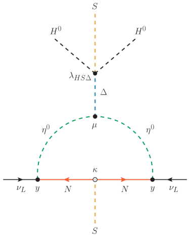
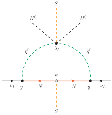
Figure 1: Neutrino mass generation in the ultraviolet (left) and low-energy theories (right). The effective $\lambda_{5}$ coupling enables the generation of neutrino masses at the 1-loop level in the low-energy theory.

Finally, we comment on neutrino masses. The breaking of the $\rm U(1)_{L}$ global symmetry generates a Majorana mass term for the $N$ fermions, $\frac{M_{N}}{2}\,\overline{N^{c}}\,N$, with

$$M_{N}=\sqrt{2}\,\kappa\,v_{S}\,.$$ (19)

In the following, we will work in the basis in which this matrix is diagonal. Therefore, $M_{N_{n}}$ (with $n=1,2,3$) represent the physical masses of the $N$ fermionic singlets and, as a consequence of this, for singlet masses above the electroweak scale, one naturally has $v_{S}\gg v_{H}$. After the electroweak and $\rm U(1)_{L}$ symmetries are broken, non-zero Majorana neutrino masses are induced at the 1-loop level, as shown in Fig. 1. The left-hand side of this figure displays the relevant diagram for the generation of neutrino masses in the ultraviolet theory, while the right-hand side shows the equivalent diagram at low energies, once $\Delta$ is integrated out and an effective $\lambda_{5}$ coupling is obtained. The resulting diagram is the usual Scotogenic loop and one obtains the well-known expression for the neutrino mass matrix

$$\left(m_{\nu}\right)_{\alpha\beta}=\frac{\lambda_{5}\,v_{H}^{2}}{32\pi^{2}}\sum_{n}\frac{y_{n\alpha}\,y_{n\beta}}{M_{N_{n}}}\left[\frac{M_{N_{n}}^{2}}{m_{0}^{2}-M_{N_{n}}^{2}}+\frac{M_{N_{n}}^{4}}{\left(m_{0}^{2}-M_{N_{n}}^{2}\right)^{2}}\log\frac{M_{N_{n}}^{2}}{m_{0}^{2}}\right]\,,$$ (20)

with $m_{0}^{2}=m_{\eta}^{2}+(\lambda_{3}+\lambda_{4})\,v_{H}^{2}/2$. This expression agrees with [6] up to a factor of $1/2$ that was missing in the original reference.

4 Phenomenological consequences

In this Section we explore some of the phenomenological consequences of our model and highlight some distinctive features, not present in the minimal Scotogenic model. In addition to the usual fields present in the Scotogenic model, the particle spectrum of the low-energy theory contains a massive CP-even scalar, $\Phi$, and a massless Goldstone boson, the majoron $J$. The presence of this new degree of freedom may have important phenomenological consequences.

Majoron couplings to charged leptons

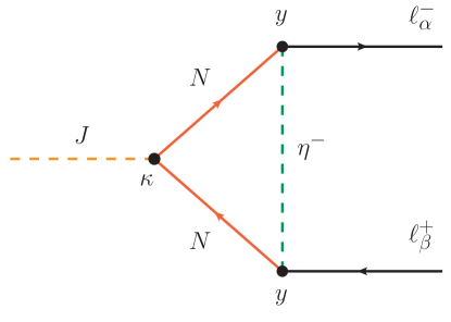
Figure 2: Loop induced majoron couplings to the SM charged leptons.

Majoron couplings to a pair of charged leptons are induced at the 1-loop level by the Feynman diagram in Fig. 2. Neglecting corrections proportional to the charged lepton massess, the resulting interaction vertex is given by

$$\mathcal{L}_{J\ell\ell}=-\frac{i\,J}{16\,\pi^{2}\,v_{S}}\,\overline{\ell}\left(M_{\ell}\,y^{\dagger}\,\Gamma\,y\,P_{L}-y^{\dagger}\,\Gamma\,y\,M_{\ell}\,P_{R}\right)\ell\,,$$ (21)

where $M_{\ell}=\text{diag}(m_{e},m_{\mu},m_{\tau})$ and we have defined

$$\Gamma_{mn}=\frac{M_{N_{n}}^{2}}{\left(M_{N_{n}}^{2}-m^{2}_{\eta^{+}}\right)^{2}}\left(M_{N_{n}}^{2}-m^{2}_{\eta^{+}}+m^{2}_{\eta^{+}}\,\log\frac{m^{2}_{\eta^{+}}}{M_{N_{n}}^{2}}\right)\delta_{mn}.$$ (22)

These results are analogous to those found in the type-I seesaw with spontaneous violation of lepton number, in which majoron couplings to charged leptons are also induced at the 1-loop level, see for instance [18].

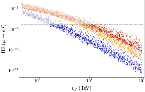
Figure 3: BR($\mu\to e\,J$) as a function of $v_{S}$ for three scenarios: $M_{N_{n}}=0.5$ TeV, $m_{\eta}^{+}\in[200,300]$ GeV (blue), $M_{N_{n}}=5$ TeV, $m_{\eta}^{+}\in[200,300]$ GeV (red) and $M_{N_{n}}=0.5$ TeV, $m_{\eta}^{+}\in[2,3]$ TeV (orange), with $\left(M_{N}\right)_{mn}=M_{N_{n}}\,\delta_{mn}$. See text for details.

The majoron off-diagonal couplings to charged leptons induce flavor violating decays, such as $\mu\to e\,J$. Using the general results derived in [19] one can obtain predictions for the model considered here. These are presented in Fig. 3, which shows BR($\mu\to e\,J$) as a function of the lepton number breaking scale $v_{S}$ for three scenarios: $M_{N_{n}}=0.5$ TeV, $m_{\eta}^{+}\in[200,300]$ GeV (blue), $M_{N_{n}}=5$ TeV, $m_{\eta}^{+}\in[200,300]$ GeV (red) and $M_{N_{n}}=0.5$ TeV, $m_{\eta}^{+}\in[2,3]$ TeV (orange), with $\left(M_{N}\right)_{mn}=M_{N_{n}}\,\delta_{mn}$. All points in this figure are compatible with neutrino oscillation data. This has been achieved by using an adapted Casas-Ibarra parametrization for the Yukawa matrix $y$ [20, 21] and taking neutrino oscillation parameters in the $3\sigma$ ranges determined by the global fit  [22]. The fermion singlet masses are set to their numerical values by fixing $\kappa$ accordingly. Finally, the scalar potential parameters have been randomly chosen, with the exception of the effective $\lambda_{5}$ coupling that is fixed to $-10^{-8}$. The horizontal dashed line displays the current experimental limit BR($\mu\to e\,J$) $<10^{-5}$ obtained by the TWIST collaboration [23]. This limit can be improved by the Mu3e experiment by looking for a bump in the continuous Michel spectrum. This strategy was recently shown to be able to rule out $\mu\to e\,J$ branching ratios above $7.3\times 10^{-8}$ at 90% C.L. [24]. Therefore, we conclude that our setup leads to observable $\mu\to e\,J$ decays, which already rule out part of the parameter space of the model and are detectable in the near future. Qualitatively similar results are obtained for the processes $\tau\to e\,J$ and $\tau\to\mu\,J$.

Collider signatures

The light CP-even scalar $h$ is identified with the $125$ GeV state discovered at the LHC, and thus we must guarantee that its properties match those observed. In particular, its production cross-section and decay modes must be (within the allowed experimental ranges) close to those predicted for a pure SM Higgs boson. This can be generally guaranteed if the mixing angle $\alpha$, defined in Eq. (13), is small. For instance, $h$ can decay invisibly via $h\to JJ$. The interaction Lagrangian of the CP-even scalar $h$ to a pair of majorons can be written as $\mathcal{L}_{hJJ}=\frac{1}{2}\,g_{hJJ}\,h\,J^{2}$, with the dimensionful coupling $g_{hJJ}$ given by

$$g_{hJJ}=v_{S}\,\lambda_{S}\,\sin\alpha+\left(\lambda_{3}^{S}-\frac{v_{H}^{2}\left|\lambda_{HS\Delta}\right|^{2}}{m_{\Delta}^{2}}\right)v_{H}\,\cos\alpha\,.$$ (23)

Using the limit on the invisible Higgs branching ratio $\text{BR}(h\to JJ)<0.11$ at $95\%$ C.L. [25], assuming that the total Higgs decay width is given by $\Gamma_{h}\approx\Gamma_{h}^{\rm SM}=4.1$ MeV [26] and taking into account that $\Gamma(h\to JJ)=g_{hJJ}^{2}/(32\,\pi\,m_{h})$, one finds $g_{hJJ}<2.4$ GeV at $95\%$ C.L.. This constraint can be easily satisfied by choosing $\lambda_{3}^{S}\lesssim 10^{-2}$. Finally, the heavy CP-even scalar $\Phi$ can also be searched for at colliders. However, for $\alpha\ll 1$ this state is mostly singlet and has very suppressed production cross-sections at the LHC.

Dark matter

The usual $\mathbb{Z}_{2}$ parity of the Scotogenic model is obtained in our model as a remnant after lepton number breaking. As a consequence of this, the lightest $\mathbb{Z}_{2}$-odd state is completely stable and can be a good DM candidate. Two scenarios emerge: (i) fermion DM, with the lighest singlet $N_{1}$ as DM candidate, and (ii) scalar DM, with either $\eta_{R}$ or $\eta_{I}$ (depending on the sign of the effective $\lambda_{5}$ coupling) as DM candidate. This is completely equivalent to the minimal Scotogenic model. However, the new scalar states at low energies can alter the DM phenomenology substantially. For instance, in the case of fermion DM, more constrained due to the strong bounds from lepton flavor violating observables, see for instance [27], it has been shown that the annihilation channels $N_{1}\,N_{1}\,\to\,\text{SM}\,\text{SM}$ and $N_{1}\,N_{1}\,\to\,J\,J$ may open up new viable regions in the parameter space of the model [28]. These s-channel processes, mediated by the CP-even scalars of the model ($h$ and $\Phi$), have a strong impact on the DM relic density, reducing the tuning normally required in the original Scotogenic model with fermion DM.

5 Summary and discussion

An ultraviolet completion for the Scotogenic model has been proposed in this letter. Our high-energy scenario contains additional degrees of freedom which, after being integrated out, give rise to the well-known low-energy Lagrangian of the Scotogenic model. In particular, they induce a naturally small $\lambda_{5}$ coupling, suppressed by two powers of the high scale $m_{\Delta}$. Our construction also generates the dark $\mathbb{Z}_{2}$ parity of the Scotogenic model, which emerges as a remnant symmetry at low energies. In summary, our ultraviolet model addresses some of the theoretical drawbacks of the original Scotogenic model.

In addition to the usual Scotogenic states, our setup predicts two additional particles at low energies: a massive scalar and a massless Goldstone boson, the majoron $J$. We have shown that they have a remarkable impact on the phenomenology of the model. New processes in flavor physics, such as $\mu\to e\,J$, are available and detectable in the near future. The dark matter phenomenology is also affected due to novel production mechanisms in the early Universe. Finally, we also expect new signatures in colliders.

While we have concentrated on a model with a global $\rm U(1)_{L}$ symmetry, it is also interesting to consider a version of our setup in which the $\mathbb{Z}_{2}$ parity has a gauge origin. In this case, the majoron would be replaced by a massive $Z^{\prime}$ boson. Furthermore, our ultraviolet completion is by no means unique and other models with similar low-energy limit exist, perhaps with different phenomenological predictions. We leave these possibilities for future work.

References

- [1] A. Zee, “A Theory of Lepton Number Violation, Neutrino Majorana Mass, and Oscillation,” Phys. Lett. 93B (1980) 389. [Erratum: Phys. Lett.95B,461(1980)].
- [2] T. P. Cheng and L.-F. Li, “Neutrino Masses, Mixings and Oscillations in Models of Electroweak Interactions,” Phys. Rev. D22 (1980) 2860.
- [3] A. Zee, “Quantum Numbers of Majorana Neutrino Masses,” Nucl. Phys. B264 (1986) 99–110.
- [4] K. S. Babu, “Model of ’Calculable’ Majorana Neutrino Masses,” Phys. Lett. B203 (1988) 132–136.
- [5] Y. Cai, J. Herrero-García, M. A. Schmidt, A. Vicente, and R. R. Volkas, “From the trees to the forest: a review of radiative neutrino mass models,” Front. in Phys. 5 (2017) 63, arXiv:1706.08524 [hep-ph].
- [6] E. Ma, “Verifiable radiative seesaw mechanism of neutrino mass and dark matter,” Phys. Rev. D73 (2006) 077301, arXiv:hep-ph/0601225 [hep-ph].
- [7] D. Hehn and A. Ibarra, “A radiative model with a naturally mild neutrino mass hierarchy,” Phys. Lett. B 718 (2013) 988–991, arXiv:1208.3162 [hep-ph].
- [8] J. Fuentes-Martín, M. Reig, and A. Vicente, “Strong problem with low-energy emergent QCD: The 4321 case,” Phys. Rev. D 100 no. 11, (2019) 115028, arXiv:1907.02550 [hep-ph].
- [9] P. Escribano, M. Reig, and A. Vicente, “Generalizing the Scotogenic model,” JHEP 07 (2020) 097, arXiv:2004.05172 [hep-ph].
- [10] G. ’t Hooft, “Naturalness, chiral symmetry, and spontaneous chiral symmetry breaking,” NATO Sci. Ser. B 59 (1980) 135–157.
- [11] E. Ma, “Derivation of Dark Matter Parity from Lepton Parity,” Phys. Rev. Lett. 115 no. 1, (2015) 011801, arXiv:1502.02200 [hep-ph].
- [12] S. Centelles Chuliá, R. Cepedello, E. Peinado, and R. Srivastava, “Scotogenic dark symmetry as a residual subgroup of Standard Model symmetries,” Chin. Phys. C 44 no. 8, (2020) 083110, arXiv:1901.06402 [hep-ph].
- [13] Y. Chikashige, R. N. Mohapatra, and R. Peccei, “Are There Real Goldstone Bosons Associated with Broken Lepton Number?,” Phys. Lett. B 98 (1981) 265–268.
- [14] G. Gelmini and M. Roncadelli, “Left-Handed Neutrino Mass Scale and Spontaneously Broken Lepton Number,” Phys. Lett. B 99 (1981) 411–415.
- [15] J. Schechter and J. W. F. Valle, “Neutrino Decay and Spontaneous Violation of Lepton Number,” Phys. Rev. D 25 (1982) 774.
- [16] C. Aulakh and R. N. Mohapatra, “Neutrino as the Supersymmetric Partner of the Majoron,” Phys. Lett. B 119 (1982) 136–140.
- [17] J. de Blas, M. Chala, M. Perez-Victoria, and J. Santiago, “Observable Effects of General New Scalar Particles,” JHEP 04 (2015) 078, arXiv:1412.8480 [hep-ph].
- [18] J. Heeck and H. H. Patel, “Majoron at two loops,” Phys. Rev. D 100 no. 9, (2019) 095015, arXiv:1909.02029 [hep-ph].
- [19] P. Escribano and A. Vicente, “Ultralight scalars in leptonic observables,” JHEP 03 (2021) 240, arXiv:2008.01099 [hep-ph].
- [20] J. A. Casas and A. Ibarra, “Oscillating neutrinos and ,” Nucl. Phys. B 618 (2001) 171–204, arXiv:hep-ph/0103065.
- [21] T. Toma and A. Vicente, “Lepton Flavor Violation in the Scotogenic Model,” JHEP 01 (2014) 160, arXiv:1312.2840 [hep-ph].
- [22] P. F. de Salas, D. V. Forero, S. Gariazzo, P. Martínez-Miravé, O. Mena, C. A. Ternes, M. Tórtola, and J. W. F. Valle, “2020 global reassessment of the neutrino oscillation picture,” JHEP 02 (2021) 071, arXiv:2006.11237 [hep-ph].
- [23] TWIST Collaboration, R. Bayes et al., “Search for two body muon decay signals,” Phys. Rev. D 91 no. 5, (2015) 052020, arXiv:1409.0638 [hep-ex].
- [24] A.-K. Perrevoort, Sensitivity Studies on New Physics in the Mu3e Experiment and Development of Firmware for the Front-End of the Mu3e Pixel Detector. PhD thesis, Ruprecht-Karls-Universität Heidelberg, 2018.
- [25] ATLAS Collaboration, “Combination of searches for invisible Higgs boson decays with the ATLAS experiment,”.
- [26] LHC Higgs Cross Section Working Group Collaboration, D. de Florian et al., “Handbook of LHC Higgs Cross Sections: 4. Deciphering the Nature of the Higgs Sector,” arXiv:1610.07922 [hep-ph].
- [27] A. Vicente and C. E. Yaguna, “Probing the scotogenic model with lepton flavor violating processes,” JHEP 02 (2015) 144, arXiv:1412.2545 [hep-ph].
- [28] C. Bonilla, L. M. G. de la Vega, J. M. Lamprea, R. A. Lineros, and E. Peinado, “Fermion Dark Matter and Radiative Neutrino Masses from Spontaneous Lepton Number Breaking,” New J. Phys. 22 no. 3, (2020) 033009, arXiv:1908.04276 [hep-ph].