Linear and nonlinear optimal growth mechanisms for generating turbulent bands

Abstract

Linear and nonlinear energy optimizations in a tilted domain are used to unveil the main mechanisms allowing the creation of a turbulent band in a channel flow. Linear optimization predicts an optimal growth for streamwse and spanwise wavenumbers $k_{x}=1.2$, $k_{z}=-1.75$, corresponding to the peak values of the premultiplied energy spectra of direct numerical simulations. At target time, the linear optimal perturbation is composed by oblique streaks, which, for a sufficiently large initial energy, induce turbulence in the whole domain, due to the lack of spatial localization. When localization is achieved by adding nonlinear effects to the optimization, or by artificially confining the linear optimal to a localized region in the spanwise direction, a large-scale flow is created, which leads to the generation of a localised turbulent band. These results suggest that inducing transition towards turbulent bands in a tilted domain, two main elements are needed: a linear energy growth mechanism such as the lift-up for generating large-amplitude flow structures which produce inflection points; large-scale vortices ensuring spatial localisation. Remarkably, these two elements alone are able to generate an isolated turbulent band also in a large, non-tilted domain.

1 Introduction

In plane Poiseuille flow, transition to turbulence often arises for Reynolds numbers not surpassing the critical value for linear stability analysis, $Re=5772$. For Reynolds numbers consistently lower than this threshold value, the flow may exhibit localised turbulence (Tsukahara et al., 2005). Carlson et al. (1982) was the first to experimentally observe laminar-turbulent patterns in the channel flow, for $Re=1000$. In very large domains, localised turbulent bands tilted with respect to the streamwise direction, plunged in the laminar flow, are observed (Tsukahara et al., 2014; Xiong et al., 2015; Tao et al., 2018; Shimizu & Manneville, 2019; Kashyap et al., 2020). This oblique laminar-turbulent pattern is also observed in other shear flows, although for a different range of Reynolds numbers and presenting different angles (Prigent et al., 2002; Barkley & Tuckerman, 2005; Duguet et al., 2010; Tuckerman & Barkley, 2011; Duguet & Schlatter, 2013; Chantry et al., 2017; Tuckerman et al., 2020). Using numerical simulations, Tao et al. (2018) have established that oblique turbulent bands may arise in the channel flow at $Re\approx 660$. Recently, forcing the flow with an inflectional instability, Song & Xiao (2020) have been able to generate turbulent bands at $Re\approx 500$, although not self-sustained. Turbulent bands have been analysed by several authors in large domains with the aim of studying their characteristics, such as their angle and length (Tsukahara et al., 2005; Tao et al., 2018; Kashyap et al., 2020), as well as their dynamics and interactions (Duguet et al., 2010; Tao et al., 2018; Shimizu & Manneville, 2019; Gomé et al., 2020). In order to reduce the computational cost and the flow complexity, Barkley & Tuckerman (2005, 2007) studied the behaviour of the plane Couette flow in a small domain tilted perpendicularly to the turbulent band direction. Later, Tuckerman et al. (2014) extended this methodology to the plane Poiseuille flow.
Recently, many works have focused on the origin and growth of turbulent bands. In a large domain, Shimizu & Manneville (2019) observed that streaks are generated at the head of the turbulent band and suggest that streak generation could be the origin of the self-sustaining process of a single turbulent band. According to this hypothesis, investigating a small domain at the head of the band, Xiao & Song (2020) have performed a linear stability analysis of the mean flow computed in three different regions at the head of the band. They have notably found that an inflectional spanwise instability generates streaky structures similar to those found at the head of a turbulent band, and they have proposed that this instability can be at the origin of the growth of the turbulent band. Based on this hypothesis, Song & Xiao (2020) have searched for a forcing that induces inflectional instability in the flow able to trigger turbulence in the form of turbulent bands. They found a fast non-modal growth associated with the base velocity profile deformed by this continuous forcing. On the other hand, using a nonlinear approach, Paranjape et al. (2020) have searched for an edge state in a tilted domain and they have found a localised nonlinear travelling wave solution that shows properties very similar to those of turbulent bands in a tilted domain. Conversely, Tao et al. (2018) suggest that, for triggering and sustaining a turbulent band, a large-scale flow is necessary. In fact, all turbulent bands are characterized by a small-scale flow inside the turbulent region, characterised by streaks and vortices, surrounded by large-scale vortices, parallel to the turbulent bands and having opposite direction on their two sides. In particular, Duguet & Schlatter (2013) have argued that the validity of the continuity equation for this large-scale flow is responsible for the turbulent band oblique evolution.
Shimizu & Manneville (2019) observed that turbulent bands are sustained by an active streak generation at the head of the bands, while streaks decay is found in the tail. Moreover, Tao et al. (2018) reported a strong increase of the total disturbance kinetic energy corresponding with the creation of turbulent bands. This energy increase follows an almost algebraic growth, instead of an exponential behaviour, as should be expected in the case of asymptotic instability as that reported by Xiao & Song (2020). It is known since the pioneer work of Landahl (1980), that an algebraic kinetic energy growth of perturbations is induced when weak counter-rotating vortices generate high-amplitude streaky structures by means of the lift-up mechanism. These two flow structures, which are easily retrieved by optimal transient growth analysis (Luchini, 2000), are two of the fundamental elements of the self-sustaining process which supports turbulence in shear flows (Hamilton et al., 1995; Waleffe, 1997), together with secondary instability of the streaks which is linked to the creation of inflectional points in the velocity profiles. Despite the observation of a consistent kinetic energy growth together with streaks generation in the head of a turbulent band, the possible relation between turbulent bands generation, the optimal energy growth of streaks and their inflectional instability, have still not been investigated in the literature.
The aim of this study is to elucidate the possible link between transient energy growth mechanisms and the generation and sustaining of turbulent bands in channel flow. For investigating the energy growth mechanism in detail, we restrain the analysis to a tilted domain allowing the generation of a single localised turbulent band, as previously done in direct numerical simulations (Tuckerman et al., 2014). In this study, we search for linear and nonlinear optimal perturbations for the channel flow in a tilted domain at $Re=1000$. We have found that transient growth of streaks is able to generate turbulent bands, although only in the presence of a large-scale flow arising from spatial localization.
The paper is organised in the following way: the problem formulation is presented in section 2. Then, in section 3 the linear and nonlinear optimal perturbations are shown and discussed. Finally, conclusions are drawn in section 4.

2 Problem formulation

For reducing the problem complexity and the computational cost, a tilted domain is considered for analysing oblique turbulent bands in plane Poiseuille flow, as previously done by Barkley & Tuckerman (2005, 2007) for plane Couette flow and by Tuckerman et al. (2014) for plane Poiseuille flow. Starting from the classical plane Poiseuille flow, $\textbf{U}_{P}=[U_{P}(y),0,0]^{T}$, with $U_{P}(y)=1-y^{2}$, defined in the coordinate system $\mathbf{x}^{\prime}=(x^{\prime},y^{\prime},z^{\prime})^{T}$, where $x^{\prime}$ indicates the direction of the flow $U_{P}$, the tilted domain is obtained by applying the following change of reference:

$$\mathbf{\hat{e}}_{x}=cos\theta\mathbf{\hat{e}}_{x^{\prime}}-sin\theta\mathbf{\hat{e}}_{z^{\prime}},\qquad\mathbf{\hat{e}}_{y}=\mathbf{\hat{e}}_{y^{\prime}},\qquad\mathbf{\hat{e}}_{z}=-sin\theta\mathbf{\hat{e}}_{x^{\prime}}+cos\theta\mathbf{\hat{e}}_{z^{\prime}},$$

$\mathbf{x}=(x,y,z)^{T}$ being the tilted domain coordinate system, and $\theta$ being the angle of the new coordinates system, corresponding to the angle of a turbulent band free to evolve in the non-tilted domain.
The dynamics of the turbulent bands in the tilted domain can be described by decomposing the instantaneous field into a perturbation $\textbf{u}^{\prime}=[u^{\prime},v^{\prime},w^{\prime}]^{T}$ and a laminar base flow $\textbf{U}=[U(y),0,W(y)]^{T}$, with $U(y)=U_{P}(y)cos\theta$ and $W(y)=U_{P}(y)sin\theta$. The perturbation dynamics is governed by the Navier-Stokes equations for incompressible flows, written in a perturbative form with respect to the base flow:

$$\frac{\partial u_{i}^{\prime}}{\partial x_{i}}=0,\qquad\displaystyle\frac{\partial u_{i}^{\prime}}{\partial t}+u_{j}^{\prime}\frac{\partial u_{i}^{\prime}}{\partial x_{j}}+u_{j}^{\prime}\frac{\partial U_{i}}{\partial x_{j}}+U_{j}\frac{\partial u_{i}^{\prime}}{\partial x_{j}}=-\frac{\partial p^{\prime}}{\partial x_{i}}+\frac{1}{Re}\frac{\partial^{2}u_{i}^{\prime}}{\partial x_{j}},$$ (1)

with $p^{\prime}$ the pressure perturbation and $Re=U_{c}h/\nu$ the Reynolds number defined using the centreline velocity of the laminar Poiseuille flow, $U_{c}$, the half width of the channel, $h$, and the kinematic viscosity $\nu$.
In order to find the optimal solution able to trigger turbulent bands in the tilted domain, we have computed linear and nonlinear optimal perturbations (Cherubini et al., 2010; Pringle et al., 2012). In both cases, we choose as objective function the energy gain $G(T)=E(T)/E(0)$, where $E(t)=1/(2V)\int u_{i}^{2}(t)dV$, $E(T)$ and $E(0)$ being the kinetic energy at the chosen target time and at the initial time, respectively. Thus, we search for the initial perturbation $\textbf{u}^{\prime}(0)$ providing the largest possible energy at fixed target time with an optimization loop based on the Lagrange multiplier technique (Cherubini et al., 2011). Linear optimization is carried out using an in-house Matlab code, whereas nonlinear optimization is implemented within the open source code $Channelflow$ (channelflow.ch) (Gibson et al. (2021)).
For all the simulations the volume flux is kept constant imposing the bulk velocity equal to $U_{bulk}=2/3$. The same domain size and spatial discretization used by Tuckerman et al. (2014) is adopted, namely $L_{x}\times L_{y}\times L_{z}=10\times 2\times 40$ discretized on $N_{x}\times N_{y}\times N_{z}=128\times 65\times 512$ grid. All computations are performed at $Re=1000$, for which Tuckerman et al. (2014) have reported a persisting turbulent-laminar patter in the form of a single band. The angle of the tilted domain, $\theta$, is chosen equal to $35^{\circ}$ in accordance with that numerically observed at $Re=1000$ by Kashyap et al. (2020) in large domains.

3 Results

(a) $k_{x}E_{uu}(k_{x})$

(b) $k_{z}E_{uu}(k_{z})$

Figure 1: (a) Isosurface of negative streamwise velocity ($u=-0.16$, yellow) and Q-criterion ($Q=0.05$) coloured by the streamwise vorticity (positive red, negative blue) of a turbulent-laminar pattern at $Re=1000$ in a domain tilted with $\theta=35^{\circ}$. (b-c) Logarithm of the premultiplied spectral energy versus the wall-normal distance $y$ for the instantaneous field in (a). The white ’X’ symbols indicate the energy peaks.

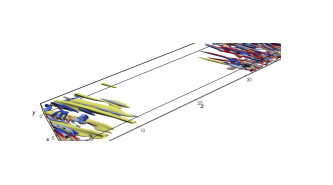
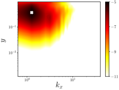
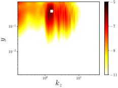
At first, a Direct Numerical Simulation (DNS) is performed at $Re=1000$ in the tilted domain. In figure 1, a snapshot of the perturbation field is shown. As previously done by other authors, the DNS is initialised with a Reynolds number for which turbulence occupies the whole domain. Then, the Reynolds number is reduced slowly until $Re=1000$, reaching the laminar-turbulent pattern shown in figure 1. As already discussed by Tuckerman et al. (2014) for a tilted domain with the same size and Reynolds number, the turbulent state appears in the form of one turbulent band. In the instantaneous field, oblique wave-like structures such as alternating low- and high-speed streaks, are observed within the turbulent band and at its head. As expected, these structures present an angle with respect to the streamwise direction comparable to that of the base flow, and resemble the streaks observed at the head of a turbulent band in large (non-tilted) domains (Shimizu & Manneville, 2019; Liu et al., 2020). Inspecting the premultiplied energy spectra of the streamwise instantaneous velocity provided in figure 1(a), 1(b), we found an energy peak at $k_{x}\approx\pm 1.27$, $k_{z}\approx\pm 1.6$. Thus, as discussed above, the flow is dominated by oblique structures with angle $\approx\arctan(k_{x}/k_{z})\approx\pm 38^{\circ}$.
In order to understand the origin of these oblique structures and the main mechanisms responsible for the generation of a turbulent band, a linear optimization of perturbations in the tilted domain is first performed. Since the base flow varies only in the wall-normal direction, the kinetic energy of the perturbations, constrained by equations (1) linearized with respect to the base flow, is optimized using a local approach, where the perturbation is supposed to be sinusoidal in the streamwise and spanwise direction, with given wavenumbers $k_{x}$ and $k_{z}$, respectively.

Figure 2: (a) Contours of the optimal gain $G$ as a function of the streamwise ($k_{x}$) and spanwise ($k_{z}$) wavenumbers, for $Re=1000$ in the domain tilted with angle $\theta=35^{\circ}$. The red cross indicates the optimal growth $G_{opt}$. (b) Streamwise velocity component of the initial optimal perturbation for $T=T_{opt}=73.11$, $k_{x}=1.2$, $k_{z}=-1.75$.

(a) Linear, $t=0$

(b) Linear, $t=T_{opt}$

(c) Nonlinear, $t=0$

(d) Nonlinear, $t=T$

Figure 3: Velocity profiles of the optimal disturbances (continuous lines). (a-b) Linear optimal for $k_{x}=1.2$, $k_{z}=-1.75$ at (a) $t=0$ and (b) $T_{opt}=73.11$. The dashed line represents the streamwise velocity profile recovered at $x=0$, $z=10$ by evolving to $t=5$ by DNS the localized initial optimal perturbation of figure 6. (c-d) Nonlinear optimal at the minimal energy able to trigger turbulence, $E_{0}=2.1\times 10^{-5}$ at (c) $t=0$ and (b) $T=10$.

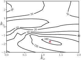
The linear optimization problem was solved at $Re=1000$ for streamwise and spanwise wavenumbers in the range $0<k_{x}<2$, $-3<k_{z}<3$. In figure 2, is provided the variation of the optimal gain with the spanwise and streamwise wavenumbers. The maximum growth is achieved at the optimal target time $T_{opt}=73.11$, for $k_{x}=1.2$ and $k_{z}=-1.75$, leading to an optimal gain $G_{opt}=195.28$. It is interesting to note that the optimal gain and time values are very similar to those found by Reddy & Henningson (1993) for the plane Poiseuille flow, although obtained for different wavenumbers. Whereas, similar values of streamwise and spanwise wavenumbers are found by Xiao & Song (2020) performing a linear stability analysis around the mean flow of a region at the head of the turbulent band. Moreover, the optimal streamwise and spanwise wavenumbers are very close to the ones for which the premultiplied energy spectra in figure 1(a), 1(b) peak. Thus, these optimal perturbations can be linked to the oblique waves observed at the head of the turbulent band. 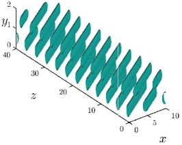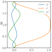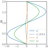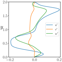As shown in figure 2, the linear optimal perturbation is oblique with angle $\arctan(k_{x}/k_{z})\approx-34.5^{\circ}$, and modulated in both streamwise and spanwise directions. This had to be expected since the base flow presents a spanwise component, in analogy with the shear flow developing on a swept-wing, whose unstable modes and optimal perturbations are characterised by cross-flow vortices, namely three dimensional oblique vortical perturbations with negative spanwise wavenumber. As shown in figure 3(a), at $t=0$ the optimal perturbation presents counter-rotating vortices with a large wall-normal component, which decreases in time towards the target time (see figure 3(b)), while the streamwise and spanwise ones strongly increase creating oblique streaks. The mechanism creating these oblique energetic structures is based on the transport of the wall-normal shear of both streamwise and spanwise component of the base flow, which may be seen as a tilted counterpart of the lift-up effect.

Figure 4: Kinetic energy time evolution for the linear optimal perturbation with $E_{0}=0.01.0.1,1$ (black lines) and for the nonlinear one (red line) for $E_{0}=2.1\times 10^{-5}$.

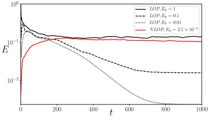
The linear optimal perturbation computed for $T_{opt}$ is then injected onto the laminar flow in the tilted domain with different values of the initial energy $E(0)$, in order to verify whether such a linear transient-growth mechanism could induce transition in the form of turbulent bands. In figure 4, the energy evolution in time is reported for the linear optimal perturbations with different initial energies (black lines). The perturbation with unitary energy norm is the only one able to induce the formation of the turbulent band, while the others lead to relaminarisation. However, it is observed that turbulence is at first triggered in the whole domain and successively localises in a band. This is mostly probably due to the fact that the linear optimal disturbance is not spatially localized but occupies the whole domain, which also explains the large amount of energy needed for triggering turbulence by means of this optimal mechanism. To provide spatial localization of the optimal perturbation, aiming at triggering the turbulent band, we extended the optimization to the fully nonlinear equations, which usually provide a consistent spatial localization (Kerswell, 2018; Cherubini et al., 2010; Farano et al., 2015). Notice that the nonlinear optimization is performed in a fully three-dimensional framework, without any hypothesis on the perturbation wavenumbers.

(a) 2D, $t=0$

(b) 3D, $t=0$

(c) 3D, $t=600$

Figure 5: Nonlinear optimal perturbation for $Re=1000$, $E_{0}=2.1\times 10^{-5}$, $T=10$. (a) Shaded isocontours of the wall-normal perturbation and vectors of the $y$-integrated flow in the $y=0.25$ plane at $t=0$. (b-c) Isosurface of negative streamwise velocity (yellow) and Q-criterion coloured by the streamwise vorticity (positive red, negative blue) for (b) $t=0$, $u=-0.01$, $Q=0.02$; (c) $t=600$, $u=-0.16$, $Q=0.05$.

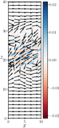
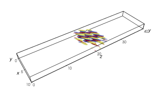
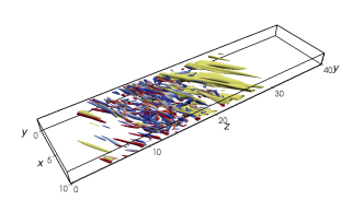
Nonlinear optimization has been performed in the tilted domain for several initial energies and target time $T=10$, which is close to the characteristic eddy turnover time of structures in the buffer layer, for which optimal streaks having the typical spanwise spacing of approximately $100$ wall units were recovered by Butler & Farrell (1993). For this target time, the nonlinear optimal perturbation triggers localised turbulence already for $E_{0}\geq 2.1\times 10^{-5}$. The nonlinear optimal perturbation at the minimal input energy able to trigger turbulence is shown in figure 5 (a-b). As expected from previous works (Cherubini et al., 2011; Monokrousos et al., 2011; Pringle et al., 2012), it is localised in the longitudinal direction. Furthermore, it presents remarkable similarities with the edge state found by Paranjape et al. (2020) in a tilted domain for $Re=760$. In figure 5(a) the isocontours of the wall-normal perturbation are reported, together with the normalised $y$-integrated large-scale flow $\overline{u_{i}}=\int_{-1}^{1}u_{i}dy$. One can observe a small-scale flow within a localised region, where the turbulent band will be generated, together with two larger-scale vortices surrounding this region, having opposite direction upstream and downstream of the localised perturbation. A large-scale vortical flow surrounding the region developing into a turbulent spot has been previously reported by several authors in both tilted and non-tilted domains. The three-dimensional visualization in figure 5(b) shows that the small-scale flow is constituted by oblique streaks flanked by counter-rotating vortices. The streaks are aligned with the base flow, presenting an angle of approximately $35^{\circ}$ with respect to the streamwise direction, in accordance with the angle of the linear optimal perturbation. 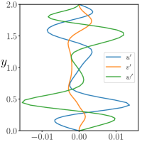As expected, this localised optimal perturbation evolves in time towards a turbulent band, as shown in figure 5(c). Notice that the nonlinear optimal perturbation induces transition for an initial energy five orders of magnitude lower than that of the linear optimal one; this cannot be exclusively due to its spatial localisation. In fact, the wall-normal velocity profiles provided in figure 3(c) present strong differences with respect to their linear counterpart shown in figure 3(a). In particular, as typically observed in nonlinear optimal perturbations (Cherubini et al., 2011), the streamwise velocity component is now of the same order of magnitude than the other ones, and the wall-normal component strongly changes. At target time (figure 3(d)) deformed streaks are obtained, presenting inflection points which might be linked to the inflectional instability discussed in Song & Xiao (2020).
To isolate the effect of spatial localisation from the strong changes in the velocity profiles induced by the nonlinear effects, we enforced localisation in the $z$ direction on the three-dimensional linear optimal solution shown in figure 2. This is achieved by multiplying the velocity components for a normal distribution having the form:

$$\textit{f}(z)=e^{-\frac{1}{2}\frac{(z-z_{0})^{2}}{\sigma^{2}}},$$

where $z_{0}=10$ represents the value at which the perturbation should be centered, and $\sigma=2.5$ is its standard deviation.

(a) $t=0$

(b) $t=20$

(c) $t=50$

(d) $t=80$

(e) $t=100$

(f) $t=150$

Figure 6: Time evolution of the localised linear optimal perturbation at different times: shaded contours of the wall-normal velocity at $y=0.25$.

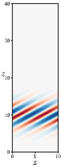
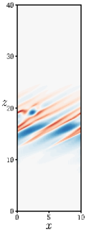
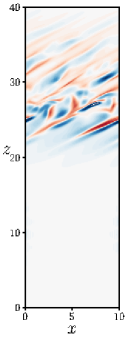
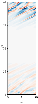
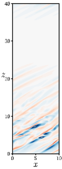
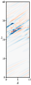
This localised perturbation is injected in the DNS with different initial energies. Its time evolution for the minimal initial energy able to induce turbulent bands, i.e., $E_{0}=3.3\times 10^{-3}$, is reported in figure 6. At first, the oblique streaks increase their amplitude ($t=20$) and start to saturate nonlinearly, until secondary instability arises ($t=50$) and triggers turbulence in a localised zone plunged in the laminar flow ($t=80-100$). At $t=150$, the flow presents the same configuration shown in figure 1 for a turbulent band generated by decreasing the Reynolds number starting from a fully turbulent velocity field. Notably, inflection points similar to those observed in figure 3(d), are observed at small time in the velocity profiles (see the dashed line on figure 3(b)). Thus, it appears that for triggering a turbulent band in the tilted domain, starting from a rather weak perturbation, two main elements are needed: small-scale oblique streaks aligned with the baseflow, that saturate creating inflection points, and a large-scale vortical flow ensuring spatial localisation in the $z$ direction. The transition at the small-scale is due to the classical lift-up mechanism, followed by secondary instability of the saturated streaks, which triggers the self-sustained cycle supporting turbulence (Hamilton et al., 1995; Waleffe, 1997). However, in the absence of a large-scale flow ensuring localisation and allowing to maintain the band, these mechanisms are not sufficient to generate localised turbulence. Of course the initial phase of growth due to the lift-up mechanism can be skipped by directly feeding the flow with inflection points, as done by Song & Xiao (2020), but at the cost of a larger amplitude disturbance, which can be more difficult and expensive to obtain in an experimental setup.
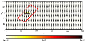
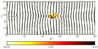
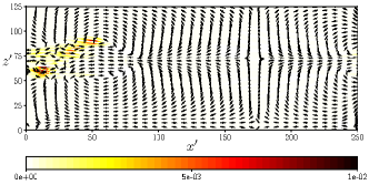
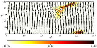
Finally, we should verify whether this artificially-localised perturbation able to optimally produce streaks, can generate turbulent bands also in large, non-tilted domains, where no angle is imposed a priori. Thus, we have reported the artificially-localised linear optimal perturbation computed in the tilted domain, in a very large (non-tilted) domain of size $L_{x^{\prime}}\times L_{y^{\prime}}\times L_{z^{\prime}}=250\times 2\times 125$, and let it evolve freely by a DNS. As shown in figure 7, despite at $t=0$ a large-scale flow is present only in the vicinity of the perturbation, at $t=100$ a clear quadrupolar large-scale vortical structure, filling the whole domain, is observed. Notice that, as discussed in Wang et al. (2020), a quadrupolar structure arises in the presence of a negative spanwise vorticity generated near the walls inside a spot, as a consequence of the shearing of the streamwise velocity and the breaking of the spanwise homogeneity. New streaky structures, generated by the self-sustained process triggered by the optimal counter-rotating vortices and streaks, are then created following the shear layer between two of the previously observed large-scale vortices ($t=300$), finally creating a clear turbulent band ($t=800$). Despite not being optimal for this large, non-tilted domain, this perturbation is able to generate a large-scale flow that promotes the formation of small-scale streaks in an oblique direction, consequently inducing the band formation. The optimization of perturbations in this large non-tilted domain is beyond the scope of the present work, and is treated in detail in Parente et al. (2021), where the minimal-energy optimal perturbations able to generate turbulent bands are computed and discussed for different values of $Re$.

(a) $t=0$

(b) $t=100$

(c) $t=300$

(d) $t=800$

Figure 7: Time evolution of the localised linear optimal perturbation reported in a large domain: contours of the wall-normal velocity and vectors of the large-scale flow ($\overline{u},\overline{w})$.

4 Conclusion

In this work we have investigated the energy growth mechanisms involved in the laminar-turbulent transition in the form of turbulent bands using linear and nonlinear optimization. We have considered a plane Poiseuille flow at $Re=1000$ in a tilted domain with angle $\theta=35^{\circ}$ that exhibits a single turbulent band. Linear optimization have reported that the optimal perturbation is three-dimensional and aligned with the oblique baseflow, in the form of low- and high- speed streaks modulated in the streamwise and spanwise directions with $k_{x}=1.2$ and $k_{z}=-1.75$, respectively. Similar wavenumbers are found at the same Reynolds number by direct numerical simulation and by linear stability analysis at the head of the turbulent band, where an angle comparable to that of the optimal streaks is observed. However, the linear optimal perturbation needs a very large initial energy to trigger turbulence, which spreads in the whole domain. Using nonlinear optimization, a localized turbulent band is triggered for an initial energy five orders of magnitude weaker, $E_{0}=2.1\times 10^{-5}$. The nonlinear optimal perturbation is characterised by a localised small-scale flow and a large-scale flow surrounding it. The small-scale flow is composed by oblique counter-rotating vortices and streaks with an angle comparable to that found via linear optimization, which develop inflection points at target time. In order to isolate the influence of large-scale flow and localization from that of the small-scale structures, we have constructed a localized perturbation by artificially confining the linear optimal to a localized region in the spanwise direction and injected it on the laminar flow both in the tilted and in a non-tilted, very large domain. In both domains, a turbulent band is created. These results suggest that transition to a turbulent band might arise due to the optimal lift-up mechanism when coupled with a large-scale vortical flow intimately linked to the spatial localisation of the disturbance. This energy growth mechanism provides high-amplitude streaks developing inflection points when saturating nonlinearly, but since the optimal streaks are aligned with the base flow, they cannot generate a turbulent band by themselves. However, the large-scale flow generated by the spatial localisation of the perturbation provides the preferential direction of spreading of the streaks generated by the lift-up mechanism, and is thus necessary to trigger turbulence in the form of turbulent bands.

[Funding]This work was granted access to the HPC resources of IDRIS under the allocation 2020- A0072A06362 and A0092A06362 made by GENCI.

[Declaration of interests] The authors report no conflict of interest.

References

- Barkley & Tuckerman (2005) Barkley, D. & Tuckerman, L. S. 2005 Computational study of turbulent laminar patterns in couette flow. Physical review letters 94 (1), 014502.
- Barkley & Tuckerman (2007) Barkley, D. & Tuckerman, L. S. 2007 Mean flow of turbulent–laminar patterns in plane couette flow. Journal of Fluid Mechanics 576, 109–137.
- Butler & Farrell (1993) Butler, K. M. & Farrell, B. F. 1993 Optimal perturbations and streak spacing in wall‐bounded turbulent shear flow. Physics of Fluids A 5 (3), 774–777.
- Carlson et al. (1982) Carlson, D. R., Widnall, S. E. & Peeters, M. F. 1982 A flow-visualization study of transition in plane poiseuille flow. Journal of Fluid Mechanics 121, 487–505.
- Chantry et al. (2017) Chantry, M., Tuckerman, L. S & Barkley, D. 2017 Universal continuous transition to turbulence in a planar shear flow. Journal of Fluid Mechanics 824.
- Cherubini et al. (2010) Cherubini, S., De Palma, P., Robinet, J-Ch & Bottaro, A. 2010 Rapid path to transition via nonlinear localized optimal perturbations in a boundary-layer flow. Physical Review E 82 (6), 066302.
- Cherubini et al. (2011) Cherubini, S., De Palma, P., Robinet, J-C & Bottaro, A. 2011 The minimal seed of turbulent transition in the boundary layer. Journal of Fluid Mechanics 689, 221–253.
- Duguet & Schlatter (2013) Duguet, Y. & Schlatter, P. 2013 Oblique laminar-turbulent interfaces in plane shear flows. Physical Review Letters 110, 034502.
- Duguet et al. (2010) Duguet, Y., Schlatter, P. & Henningson, D. S. 2010 Formation of turbulent patterns near the onset of transition in plane couette flow. Journal of Fluid Mechanics 650, 119.
- Farano et al. (2015) Farano, M., Cherubini, S., Robinet, J.-C. & De Palma, P. 2015 Hairpin-like optimal perturbations in plane poiseuille flow. Journal of Fluid Mechanics 775.
- Gibson et al. (2021) Gibson, J. F., Reetz, F., Azimi, S., Ferraro, A., Kreilos, T., Schrobsdorff, H., Farano, M., Yesil, A. F., Schutz, S. S., Culpo, M. & Schneider, T. M 2021 Channelflow 2.0. in preparation .
- Gomé et al. (2020) Gomé, S., Tuckerman, L. S & Barkley, D. 2020 Statistical transition to turbulence in plane channel flow. Physical Review Fluids 5 (8), 083905.
- Hamilton et al. (1995) Hamilton, J. M., Kim, J. & Waleffe, F. 1995 Regeneration mechanisms of near-wall turbulence structures. Journal of Fluid Mechanics 287, 317–348.
- Kashyap et al. (2020) Kashyap, P. V., Duguet, Y. & Dauchot, O. 2020 Flow statistics in the transitional regime of plane channel flow. Entropy 22 (9), 1001.
- Kerswell (2018) Kerswell, R.R. 2018 Nonlinear nonmodal stability theory. Annual Review of Fluid Mechanics 50 (1), 319–345.
- Landahl (1980) Landahl, MT 1980 A note on an algebraic instability of inviscid parallel shear flows. Journal of Fluid Mechanics 98 (02), 243–251.
- Liu et al. (2020) Liu, J., Xiao, Y., Zhang, L., Li, M., Tao, J. & Xu, S. 2020 Extension at the downstream end of turbulent band in channel flow. Physics of Fluids 32 (12), 121703.
- Luchini (2000) Luchini, P. 2000 Reynolds-number-independent instability of the boundary layer over a flat surface: optimal perturbations. Journal of Fluid Mechanics 404, 289–309.
- Monokrousos et al. (2011) Monokrousos, A., Bottaro, A., Brandt, L., Di Vita, A. & Henningson, D. S. 2011 Nonequilibrium thermodynamics and the optimal path to turbulence in shear flows. Physical review letters 106 (13), 134502.
- Paranjape et al. (2020) Paranjape, C. S., Duguet, Y. & Hof, B. 2020 Oblique stripe solutions of channel flow. Journal of Fluid Mechanics 897.
- Parente et al. (2021) Parente, E., Robinet, J.C., De Palma, P. & Cherubini, S. 2021 Minimal seeds for turbulent bands. Journal of Fluid Mechanics submitted to.
- Prigent et al. (2002) Prigent, A., Grégoire, G., Chaté, H., Dauchot, O. & van Saarloos, W. 2002 Large-scale finite-wavelength modulation within turbulent shear flows. Physical review letters 89 (1), 014501.
- Pringle et al. (2012) Pringle, C. C. T., Willis, A. P. & Kerswell, R. R. 2012 Minimal seeds for shear flow turbulence: using nonlinear transient growth to touch the edge of chaos. Journal of Fluid Mechanics 702, 415–443.
- Reddy & Henningson (1993) Reddy, S. C. & Henningson, D. S. 1993 Energy growth in viscous channel flows. Journal of Fluid Mechanics 252, 209–238.
- Shimizu & Manneville (2019) Shimizu, M. & Manneville, P. 2019 Bifurcations to turbulence in transitional channel flow. Physical Review Fluids 4 (11), 113903.
- Song & Xiao (2020) Song, B. & Xiao, X. 2020 Trigger turbulent bands directly at low reynolds numbers in channel flow using a moving-force technique. Journal of Fluid Mechanics 903, A43.
- Tao et al. (2018) Tao, J.J., Eckhardt, B. & Xiong, X.M. 2018 Extended localized structures and the onset of turbulence in channel flow. Physical Review Fluids 3 (1), 011902.
- Tsukahara et al. (2014) Tsukahara, T., Kawaguchi, Y. & Kawamura, H. 2014 An experimental study on turbulent-stripe structure in transitional channel flow. arXiv preprint arXiv:1406.1378 .
- Tsukahara et al. (2005) Tsukahara, T., Seki, Y., Kawamura, H. & Tochio, D. 2005 Dns of turbulent channel flow at very low reynolds numbers. In Fourth International Symposium on Turbulence and Shear Flow Phenomena. Begel House Inc.
- Tuckerman & Barkley (2011) Tuckerman, L. S & Barkley, D. 2011 Patterns and dynamics in transitional plane couette flow. Physics of Fluids 23 (4), 041301.
- Tuckerman et al. (2020) Tuckerman, L. S, Chantry, M. & Barkley, D. 2020 Patterns in wall-bounded shear flows. Annual Review of Fluid Mechanics 52.
- Tuckerman et al. (2014) Tuckerman, L. S., Kreilos, T., Schrobsdorff, H., Schneider, T. M. & Gibson, J. F. 2014 Turbulent-laminar patterns in plane poiseuille flow. Physics of Fluids 26 (11), 114103.
- Waleffe (1997) Waleffe, F. 1997 On a self-sustaining process in shear flows . Phys. Fluids 9, 883–901.
- Wang et al. (2020) Wang, Z., Guet, C., Monchaux, R., Duguet, Y. & Eckhardt, B. 2020 Quadrupolar flows around spots in internal shear flows. Journal of Fluid Mechanics 892, A27.
- Xiao & Song (2020) Xiao, X & Song, B. 2020 The growth mechanism of turbulent bands in channel flow at low reynolds numbers. Journal of Fluid Mechanics 883.
- Xiong et al. (2015) Xiong, X., Tao, J., Chen, S. & Brandt, L. 2015 Turbulent bands in plane-poiseuille flow at moderate reynolds numbers. Physics of Fluids 27 (4), 041702.