Steady states and phase transitions in heterogeneous asymmetric exclusion processes
Abstract
We study the nonequilibrium steady states in totally asymmetric exclusion processes (TASEP) with open boundary conditions having spatially inhomogeneous hopping rates. Considering smoothly varying hopping rates, we show that the steady states are in general classified by the steady state currents in direct analogy with open TASEPs having uniform hopping rates. We calculate the steady state bulk density profiles, which are now spatially nonuniform. We also obtain the phase diagrams in the plane of the control parameters, which though have phase boundaries that are in general curved lines, have the same topology as their counterparts for conventional open TASEPs, independent of the form of the hopping rate functions. This reveals a type of universality, not encountered in critical phenomena. Surprisingly and in contrast to the phase transitions in an open TASEP with uniform hopping, our studies on the phase transitions in the model reveal that all the three transitions are first order in nature. We also demonstrate that this model admits delocalised domain walls (DDWs) on the phase boundaries demarcating the generalised low and high density phases in this model. However, in contrast to the DDWs observed in an open TASEP with uniform hopping, the envelopes of the DDWs in the present model are generally curved lines.
I Introduction
Many natural systems are driven by some external fields or are made of self-propelled particles. In the long time limit, these systems evolve into stationary states which carry steady currents, which are hallmarks of nonequilibrium systems. Such states are characterised by a constant gain or loss of energy, which distinguishes them from systems in thermal equilibrium. Examples of such driven systems range from live cell biological systems like ribosomes moving along mRNA or motor molecules “walking” along molecular tracks known as microtubules to ions diffusing along narrow channels, or even vehicles traveling along roads. In order to elucidate the nature of such nonequilibrium steady states and in the absence of a general theoretical framework, it is useful to study purpose-built simple models. To this end, a variety of driven lattice gas models have been introduced and studied extensively basic .
In this work, we focus on driven one-dimensional (1D) models with open boundaries, where particles preferentially move in one direction. In particular, we work on the totally asymmetric simple exclusion process (TASEP), that has become one of the paradigms of nonequilibrium physics in low-dimensional systems (see, e.g., Ref. tasep-rev for reviews). In this model identical particles hop unidirectionally and with a uniform rate along a 1D lattice krug . The hopping movement is subject to exclusion, i.e., when the target site is empty, since a given site can accommodate maximum one particle. Particles enter the system at one side at a specified rate , and leave the system through the other end at a given rate ; and are the two control parameters of TASEP. It is known that the steady states of TASEPs with open boundaries are rather sensitive to the boundary conditions: by varying the boundary conditions, i.e., by varying , the steady states of open TASEPs can be varied, resulting into boundary-induced nonequilibrium phase transitions. These are genuine nonequilibrium effects, since equilibrium systems are usually insensitive to precise boundary conditions.
In the original TASEP model, the hopping rate in the bulk is assumed to be a constant (of unit value), which is of course an idealisation. In real life examples it is generally expected to have nonuniformity along the bulk of the TASEP channel leading to nonuniform hopping rates. For instance, mRNA in cells are known to have pause sites, where the effective hopping rates are lower pause . This is a potentially important issue even in urban transport, where the speeds of vehicles (which is the analogue of the hopping rates here) depend sensitively on the bottlenecks along the roads transport . Such spatially varying hopping rates can either be smoothly varying along the TASEP lanes, or be random quenched disorders with given distribution. We focus here on the case with smoothly varying hopping rates, for which the generic nature of the steady states in TASEPs are still not known. There have been some studies on quenched heterogeneous TASEP; see, e.g., Refs. qtasep1 ; qtasep for previous studies on different aspects of heterogeneous TASEP. Recently, how the steady states of TASEPs with periodic boundary conditions are affected by smoothly varying hopping rates are studied prr ; see also Ref. astik-prr for a study on periodic TASEP with random quenched disordered hopping rates. A type of universality has been uncovered, showing the topological equivalence of the phase diagrams independent of the precise form of the space dependence of the hopping rates. More recently, an inhomogeneous -TASEP with open boundaries has been proposed in the context of ribosome movements along messenger RNA strands erdmann . Using a hydrodynamic approach erdmann , this study reveals complex natures of the steady states and the phase transitions. In the present work, we revisit the problem of open TASEPs with spatially non-uniform hopping rates, which corresponds to the limit of the model studied in Ref. erdmann . Following Ref. prr , we set up the analytical mean-field theory (MFT) framework to calculate the steady state density profiles for generic smoothly varying hopping rates. We illustrate the theoretical predictions by calculating the density profiles for a few representative examples of spatially varying hopping rates in Monte-Carlo simulation (MCS) studies. The MFT that we develop complements the hydrodynamics-based approach developed in Ref. erdmann , and helps to understand the applicability and limitations of MFT in heterogeneous TASEPs, an important theoretical and technical issue given MFT’s prevalence and general popularity as a theoretical tool to study exclusion processes. Within this MFT, by defining an order parameter reminiscent of the same in open TASEPs but independent of the forms of the space dependent hopping rates, we are able to clearly connect the quantitative difference between the phase diagrams obtained here with those for open TASEPs with uniform hopping. We further study the nonequilibrium phase transitions in the model. Our MCS studies show that all the phase transitions are first order or discontinuous in nature, a surprising and unexpected outcome from this work, that is easily explained within the MFT we develop here. This is in contrast to an open TASEP with uniform hopping. Our extensive MCS studies on the domain walls reveal their delocalised nature, qualitatively similar to those found in an open uniform TASEP. Nonetheless, our studies point out how the effects of the nonuniform hopping get visible in the form of the envelope of the moving domain wall, which is now a nonlinear function of position along the TASEP channel. The rest of the article is organised as follows. In Sec. II we define and construct our model. Next, in Sec. III.1 we discuss the algorithm of the MCS study of the model to numerically calculate the steady state densities. Then in Sec. III.2, we set up the MFT, and solve it to obtain the steady state densities for smoothly varying hopping rates, and compare with our MCS results. In Sec. III.3, we present the phase diagrams of the model. Then in Sec. IV, we discuss the phase transitions in the model. We summarise our results in Sec. V.
II Model
The model consists of a 1D lattice of size . The particles enter through the left end at rate , hop unidirectionally from the left to the right, all subject to exclusion, i.e., a single site can accommodate maximum one particle at a time, and finally leave the system at a rate . Labelling each site by an index that runs from 1 to , the hopping rate at site is given by ; see Fig. 1 for a schematic model diagram.

A microscopic configuration of the model is characterised by a distribution of identical particles on the lattice, i.e., by configurations , where each of the occupation numbers is equal to either zero (vacancy) or one (particle), as it should be in a model with exclusion. Physically, a hard core repulsion between the particles is imposed, resulting into prohibition of a double or higher occupancy of sites in the model. The full state space then consists of configurations. The following elementary processes fully define the microscopic dynamical update rules of this model:
(a) At any site a particle can jump to site if unoccupied with a rate .
(b) At the site a particle can enter the lattice with rate only if it is unoccupied; and
(c) At the site a particle can leave the lattice with rate when it is occupied.
In general, for . Processes (a)-(c) formally define a TASEP with open boundary conditions. If all of for all identically, then this model reduces to the conventional TASEP with open boundary conditions tasep-rev . We consider some specified choices of that depends explicitly on , and study their effects on the nonequilibrium steady states of the model. Recall that the steady states of an open TASEP with and as the entry and exit rates, and a uniform hopping rate are characterised by the mean bulk density : For and , one has giving the low density (LD) phase, for and , one has giving the high density (HD) phase, and for , one has giving the maximal current (MC) phase. This immediately gives the phase boundary in the plane tasep-rev . The principal aim of the present study is to find the phases, phase boundaries and the nature of the associated phase transitions, and the principles behind obtaining them when the hopping rate is not constant, but spatially smoothly varying.
III Steady-state densities
We are interested to calculate the density profiles in the steady states. To this end, we set up MFT which can be solved analytically. We supplement the MFT results by extensive Monte-Carlo simulations (MCS).
III.1 Monte-Carlo simulations
We consider a lattice of sites, labelled by an index with . Let , which is either 0 or 1, be the occupation at site at time . We perform MCS studies of the model subject to the update rules (a)-(c) described above in Sec. II by using a random sequential updating scheme. The particles enter the system through the left most site () at a fixed rate , subject to exclusion, i.e., if . After hopping through the system from to , subject to exclusion, the particles exit the system from at a fixed rate . Here, and are the two simulation parameters, which are varied to produce different steady states. After reaching the steady states, the density profiles are calculated and temporal averages are performed. This produces time-averaged, space-dependent density profiles, given by ,which are parametrised by and ; here implies temporal averages over steady states. The simulations have been performed with up to Monte-Carlo steps. Lastly, all the measurements are made in the steady states, which are reached by the system after spending certain transient times. In an open TASEP, a steady state is easily ascertained by observing the spatio-temporal constancy of the average density (excluding the domain walls) in the bulk of the system. In the present problem, such a way to confirm the steady state fails due to the (expected) spatially varying steady state density in the bulk. Instead, we use the constancy of the current in the steady state, a condition that holds both in the present study and also for a uniform open TASEP. In our MCS studies, all our measurements are done only after this condition is satisfied.
III.2 Mean-field theory
The dynamics of TASEP is formally given by rate equations for every site which are not closed. In MFT approximation, we neglect correlation effects and replace the average of product of densities by the product of average of densities blythe . While this is an approximation, this has worked with high degree of accuracy in the original TASEP problem and its many variants (see, e.g., Refs. erwin-lk ; niladri1 ; tirtha1 as representative examples); we use MFT here as a guideline in our analysis below. The dynamical equation for is given by
| (III.1) |
for a site in the bulk. Clearly, Eq. (III.1) is invariant under the transformation together with and , which is the particle-hole symmetry of this model erwin-lk .
To proceed further in the MFT approximation, we label the sites by and take , which makes a continuous variable between 0 and 1: . In this parametrisation, the hopping rate function is given by , that is assumed to vary slowly in . We define a lattice constant , where is the geometric length of the system. To simplify notation, we fix the total length to unity without any loss of generality. In the thermodynamic limit , is a small parameter. Further, we define as the steady state density at . In the steady state, we expand the different terms on rhs of (III.1) in a Taylor series in powers of . We get
| (III.2) | |||||
| (III.3) | |||||
Substituting the above and retaining up to , we get
| (III.4) |
neglecting terms higher order in . Equation (III.4) allows us to extract a bulk current given by
| (III.5) |
which must be a constant independent of in a given steady state. That Eq. (III.4) has the form of an equation of continuity is no surprise - this is because away from the boundaries in the bulk of the TASEP, particles only hop from left to right, subject to exclusion, which keeps the particle number locally conserved. In the continuum limit, and hence the average current is
| (III.6) |
valid when and are sufficiently smooth. It is evident that the MFT equations (III.4)-(III.6) are invariant under the particle-hole symmetry discussed above. Due to this property it is enough to restrict the analysis to the LD and MC phase density profiles; the HD phase density can be constructed from the LD phase density by using the particle-hole symmetry. Notice that this MFT does not capture any time-dependent or dynamical information, unlike hydrodynamic approaches. Nonetheless, considering the inherent simplicity of our MFT and the general popularity of MFT as a theoretical tool to study TASEPs, it is useful to study the steady states of this model by MFT, which serves as a good benchmark of the success, applicability and limitations of the mean field approaches vis-á-vis other approaches like hydrodynamic methods.
General solutions of the density in MFT:-
We now derive the generic steady state density profiles and delineate the phases by using the MFT equation (III.6). In this study, we closely follow the method outlined in Ref. prr , that was subsequently extended to and refined for interacting systems arvind1 ; arvind2 . As argued below, these solutions holds for any smoothly varying . Equation (III.6) is a quadratic equation in . In Eq. (III.6) since is a constant and has an explicit -dependence, must be -dependent, such that the product of the various factors on the rhs of (III.6), all of which are individually -dependent, produces an -independent result . Equation (III.6) has two spatially nonuniform solutions and for a given :
| (III.7) | |||
| (III.8) |
for any . Evidently, both and are continuous functions of , as long as itself is a continuous function of . Further, everywhere, whereas everywhere. Clearly, if is a constant then is also a constant, independent of (ordinary TASEP with uniform hopping). At this stage is still unknown. Since is real (in fact positive definite) everywhere, we must have giving an upper bound on :
| (III.9) |
Inequality (III.9) must hold for all . Clearly, has a maximum given by
| (III.10) |
for a given ; see also Ref. krug11 for an analogous result in a disordered exclusion process. Note that is the maximum possible current that can be sustained by the system for all possible choices of the control parameters . However, may not reach for any ; see below. In the limit of uniform hopping with everywhere, , corresponding to the MC phase current in the conventional TASEP. We thus note that in the present model steady states with current for a given should generalise the standard MC phase in open TASEPs with uniform hopping.
We now systematically derive the conditions for the different phases. To do this, we must calculate to specify the solutions and completely.
Recall that in the LD phase of conventional open TASEPs with uniform hopping, the steady state is described by the incoming current, which in the bulk is given by , the outgoing current. This corresponds to as the bulk density in the LD phase. In contrast, in the HD phase, , giving as the HD phase bulk density; a superscript refers to an open TASEP with uniform hopping. The MC phase is associated with the current in the bulk. The LD-HD phase boundary is given by the condition giving ; the LD-MC and HD-MC phase boundaries likewise are given by and , giving, respectively, and as the phase boundaries. We now generalise this picture by finding out the forms of in the present problem.
LD phase:-
We start by noting that the current in the bulk of the TASEP channel is , where is or . Since , we obtain
| (III.11) |
Since, the steady state bulk density in the LD phase is less than 1/2 everywhere, the density profile in the LD phase is given by
| (III.12) |
Then we must have as in an open TASEP with a uniform hopping rate. Equation (III.12) gives the steady state density in the LD phase for a given and depends on the entry rate , but not on the exit rate , as expected in the LD phase. With everywhere, , neglecting the other solution for for an open TASEP with a uniform hopping rate.
We have plotted versus in Fig. 2 for two different and simple choices of the hopping rate function :
| (III.13) | |||||
Clearly, in Choice I is symmetric about , whereas in Choice II has no particular symmetry. Results on the steady state densities from MFT and MCS studies are plotted together in Fig. 2, which show good agreements between MFT and MCS results.
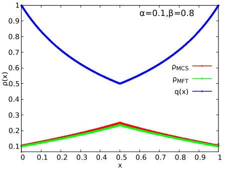
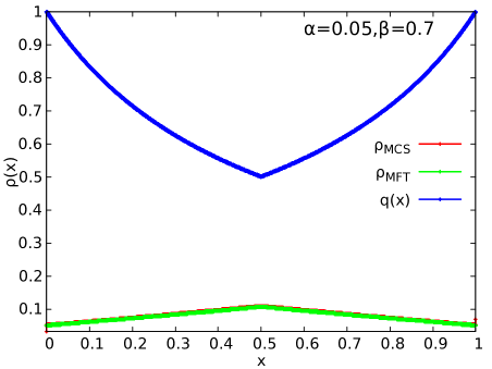
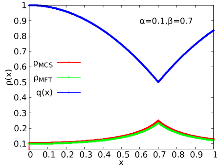
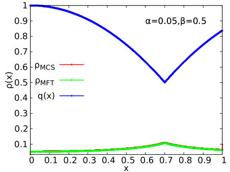
HD phase:-
The logic we have developed above to obtain can be used to obtain , the steady state density in the HD phase. Noting that , we obtain the HD phase current
| (III.15) |
Since, the steady state bulk density everywhere is more than 1/2, the density profile in the HD phase is given by
| (III.16) |
Therefore, we must have as for an open TASEP with uniform hopping. In contrast to , given by (III.12) above, in (III.16) depends on and the exit rate , but not on , as expected in the HD phase. With everywhere, , neglecting the other solution for an open TASEP with a uniform hopping rate.
In an open TASEP with uniform hopping, and specify the LD phase, whereas and specify the HD phase. What are the analogous conditions here? These conditions in the present case may be obtained by considering the steady state currents. We recall that the above conditions for the LD and HD phases in an open TASEP with uniform hopping can be recast in terms of the steady state currents as and for the LD phase, and and for the HD phase. These conditions may be generalised to the present case with non-uniform hopping. The LD phase now exists for
| (III.17) |
Similarly, for the HD phase to exist we must have
| (III.18) |
We have plotted versus in Fig. 3 for as defined in Choice I above. The HD phase density plots for as given in Choice II above, likewise, can be obtained from corresponding plots in the LD phase by using the particle-hole symmetry. Results from MFT and MCS studies are plotted together in Fig. 3, which again reveal good agreements between MFT and MCS results.
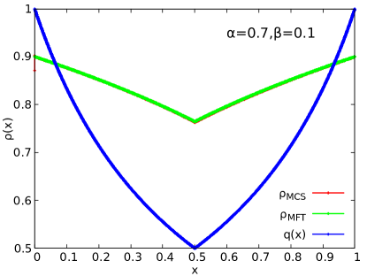
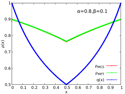
At this stage, we note that the MFT density expressions agree with the predictions from the hydrodynamic theory erdmann .
MC phase:-
The steady density in the MC phase, is somewhat tricky to calculate. We already know that the steady state current in the MC phase
| (III.19) |
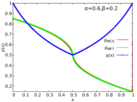
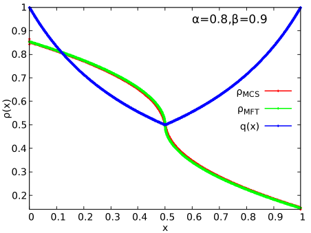
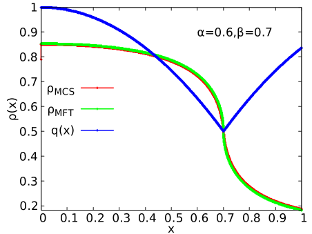
which can be used either in or , with these two solutions become identical (=1/2) at , at which point . MCS studies reveal that a part of is bigger than 1/2, whereas elsewhere it is smaller than 1/2. Thus in order to construct , we must use both and , i.e., is a combination of and , with the two segments meeting at . Whether or is to be used to construct the left or right segments (with respect to ) remains undetermined in MFT, revealing a limitation of MFT vis-á-vis hydrodynamic approaches. One can of course use the MCS result as an input at this stage. However, we can instead use heuristic arguments to settle this. To proceed, we note that the model can be imagined to be composed of two inhomogeneous TASEPs and respectively on the left and right of , which are joined at . We can now determine the densities and phases of and separately, combining which the density profile along the full TASEP channel in its MC phase can be obtained. To proceed further, we note that at , the hopping rate from to is . Furthermore, the densities at the “exit” and “entry” points (both of which are nothing but ) of and are 1/2, since (see above). In addition, and have no boundary layers at , i.e., no boundary layers at their exit and entry points, respectively. Since in the MC phase there is one boundary layer at each of and , and have boundary layers at their “entry” (i.e., ) and “exit” (i.e., ), respectively. Let us now focus specifically on . Consider first that the density profile of a uniform open TASEP at its HD-MC phase boundary is given by (corresponding to a steady state current of value 1/4) with a boundary layer at the entry end (i.e., for ) and no boundary layer at the exit end (i.e., for ). In analogy then the density profile of the segment should actually resemble the density profile of a nonuniform open TASEP at its HD-MC phase boundary. This implies that in , i.e., for , should be given by with . To find out the density profile in the remaining part, i.e., the density profile for , we now apply similar arguments on . This gives that the density in the segment should actually correspond to the density in an open nonuniform TASEP at the boundary between its LD and MC phases. Hence, its density profile should be given by with , which holds for . Now combining the densities in and , on the whole, therefore , the density profile in the MC phase of the present model, is given by between 0 and , and between and 1. Alternatively, we can directly appeal to the fact that in an open TASEP with uniform hopping in its MC phase, and blythe . Since the general solution for in the MC phase with an arbitrary must reduce to the well-known solution of the density in an open uniform TASEP in its MC phase when the space-dependence of gets progressively weaker as approaches a constant, in order to construct in our case, we should use to the left of and to its right. Both the above heuristic arguments agree well with our MCS results; see Fig. 4 for plots of versus for two choices of , each of which agrees with the MFT results. Hydrodynamic approaches such as the one developed in Ref. erdmann should provide a more formal basis to our above heuristic arguments. Our analysis here further implies that if , the location of is not in the bulk, but at the extreme ends (i.e., ), will consist of only or . Interestingly, this means in general the average density in the MC phase (averaged over the whole TASEP) can be more or less than 1/2! This is clearly in contrast to TASEP with uniform hopping, where the average density in the MC phase is 1/2.

III.3 Phase diagram
We now discuss the conditions to obtain the phase diagram and the phase boundaries in the -plane. First consider the boundary between the LD and HD phases. In the LD phase, the bulk current is given by in (III.11), whereas the bulk current in the HD phase is given by in (III.15). The two phases meet when , which gives the phase boundary between the LD and HD phases that has the form
| (III.20) |
This is a quadratic equation in in terms of with two solutions :
| (III.21) |
where , which can be bigger or smaller than unity. Since for the HD phase, gives the LD-HD phase boundary. Phase boundary (III.21) automatically reduces to , the well-known result for the phase boundary or the coexistence line between the LD and HD phases in an open TASEP with a uniform . In fact, even with nonuniform , is the phase boundary, so long as is maintained, independent of the actual profile of .
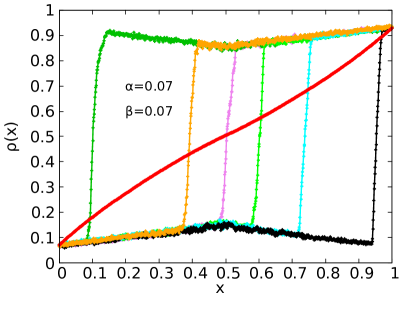
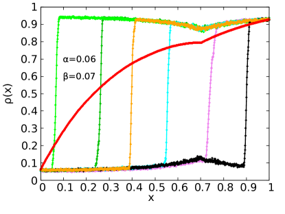
The steady state density profile at the LD-HD coexistence line has a special structure. In an open TASEP with uniform hopping rate, it occurs on the line in the plane, and is actually a delocalised domain wall (DDW), which is a domain wall or a density “shock” whose position is not fixed but fluctuates along the whole length of the TASEP length. Moreover, the position of the domain wall is equally likely to be anywhere in the TASEP. This means the long time average of the density profile, that essentially captures the envelope of the DDW, is an inclined straight line connecting at the entry end and at the exit end. Since the MFT neglects all fluctuations, it cannot capture this DDW. We numerically investigate the analogue of a DDW in a uniform open TASEP in the present problem for in Choice I, which is symmetric about the mid-point , and in Choice II, which is not symmetric about the mid-point, as given above (III.13) and (III.2), respectively. For Choice I the coexistence line in the plane is still given by due to the symmetry of the function chosen. In contrast, for Choice II there is no such symmetry, and hence the LD-HD phase boundary in the plane is given by ; see Eq. (III.21) above. Evidently, this is not a straight line in the plane. In the absence of any localising mechanism like particle non-conservation in the bulk erwin-lk , or global particle number conservation niladri1 ; prr , we expect to observe a DDW. However, space-dependent hopping rates imply that the domain wall should spend statistically unequal time at different positions in the bulk of the TASEP channel, which suggests a generic curvilinear envelope of the DDW under long-time averaging. Going beyond MFT by taking into account of fluctuations should allow us write down a Fokker-Planck equation for the instantaneous position of the density shock erwin-epje . Solving this equation one can in principle determine the mathematical form of the envelope, which is outside the scope of the present study. Instead, we investigate the shape of the DDW envelope by extensive MCS studies. Due to the diffusive nature of the DDW fluctuations, good statistics for the DDW envelope requires averaging over MCS steps. Because of this, we have restricted this particular study to with in Choice I and Choice II. To ascertain the shape of the long-time averaged envelope of the DDW, we average over MCS steps. Furthermore, in order to resolve the instantaneous (i.e., time-dependent) structures of the DDWs, we also calculate by averaging over short time windows of MCS steps. The corresponding kymographs are also obtained. To generate sufficiently smooth plots, the kymographs are indeed coarse-grained over a mesoscopic lengh . This mesoscopic length used to draw a kymograph, i.e. the length over which the spatial averaging is done, should necessarily be much smaller than the system size . We have used in our simulations.
We present our results on in Fig. 5 and Fig. 6, respectively, for in Choice I and Choice II. The corresponding kymographs are shown in Fig. 7 and Fig. 8, respectively.
We make the following conclusions from our MCS results. First of all, both the kymographs qualitatively reveal that the domain walls are delocalised for both the choices of . In order to make quantitative understanding of the DDWs, we now consider the density profile plots as shown in Fig. 5 and Fig. 6. Unsurprisingly, the short-time averages in both Fig. 5 and Fig. 6 reveal sharp, discontinuous structures of , which are reminiscent of a localised domain wall (LDW) in heterogeneous TASEPs in ring geometries prr ; niladri1 , for both choices of . The corresponding long-time averages as expected are nonlinear functions of position . Nonetheless, these long time averages reveal important distinctions between these two choices of . For instance with Choice I, the DDW envelope shows weak departure from an inclined straight line. In addition, careful observation reveals that the envelope takes a distinct shape close to , which is the location of , than away from it. In contrast for Choice II, shows a strong nonlinear behaviour with , and again shows a particular structure at , the location of , distinct from elsewhere. Lastly, the alert reader may notice that a general consequence of the nonlinear -dependence of the DDW envelopes is that the short-time averages of the densities, though display sharp discontinuities, do not have constant densities on either side of the discontinuities; see Fig. 5 and Fig. 6. Naturally, these short-time averaged density profiles are intrinsically different from the standard heaviside step functions. At a qualitative level, we can make the following conclusion. Given that the domain wall should execute random walk along the TASEP lane, the form of the domain wall envelope for an asymmetric strongly suggests that the domain wall spends different amount of time in different regions of the nonuniform TASEP lane, mimicking a random walk in a potential with a complex shape. This may be quantitatively analysed further by calculating the general profile of the DDW envelope including its shape near the minimum of analytically by going beyond MFT approaches for a given prr ; erwin-epje . This will be discussed elsewhere.


Similar considerations allow us to obtain the LD-MC and HD-MC phase boundaries. For example, the LD-MC phase boundary is given by the condition , which gives
| (III.22) |
since for the LD phase. Assuming for some in the bulk, the effect of a nonuniform is to shift the boundary line (III.22) towards the -axis. Likewise, the HD-MC phase boundary is given by the condition , giving
| (III.23) |
since for the HD phase. Again with for some in the bulk, the effect of a nonuniform is to shift the boundary line (III.23) towards the -axis. The three phase boundaries meet at . Since , the general effect of a nonuniform hopping rate appears to be to enlarge the MC phase region and shrink the LD and HD phase regions in the -plane. Furthermore, since in general, the phase diagram could be asymmetric under interchange of and . Phase diagrams for in Choice I and in Choice II are shown in Fig. 9 (top) and Fig. 9 (bottom), respectively. Phase boundaries (III.21), (III.22) and (III.23) calculated from MFT, and the corresponding results from MCS studies are superposed. Good agreement between the two are found.
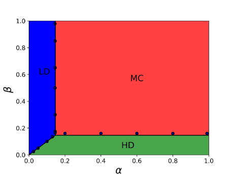
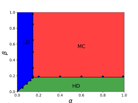
Let us now make some general observations on the phase diagrams in Fig. 9. Clearly, the phase diagrams in Fig. 9 are quantitatively different from the well-known phase diagram of an open TASEP with uniform hopping. First of all, the MC region of the phase diagrams is now distinctly bigger with space-dependent than in the corresponding phase diagram with a constant hopping rate. Secondly, between the two phase diagrams presented in Fig. 9, the one with as given in Choice I above with [Fig. 9 (top)] remains unchanged under the interchange of and , same as for the phase diagram for an open TASEP with uniform hopping rate. In contrast, the phase diagram with as given in Choice II, such that , [Fig. 9 (bottom)] has no such symmetry under the interchange of and . These properties are consistent with our discussions above; see Eqs. (III.21), (III.22) and (III.23). This firmly establishes the connections between the quantitative forms of the phase diagrams with the different choices of the hopping rate functions, a key quantitative outcome from the present study. Nonetheless, the phase diagrams above have the same topology as that for an open TASEP with uniform hopping: all of them have three phases, which meet at a common point, establishing a degree of universality in the phase diagrams that complements the results of Ref. prr .
IV Phase transitions
The original TASEP model with open boundaries and uniform hopping, the transition between the LD and HD phases are first order transitions, whereas those between the MC and LD or HD phases are second order transitions. The difference in the average bulk densities of the two phases serves as the order parameter in each of these transitions. In order to study the phase transitions in the present model, we first need to define the order parameter appropriately. To start with, we define the mean density
| (IV.1) |
for the phase , where LD, HD or MC phase. Since in the bulk of the system, necessarily. Similarly, necessarily. Interestingly, need not be 1/2, in contrast to conventional open TASEPs with uniform hopping. In fact, in the present study, with in Choice I above, comm1 due to the symmetry of and hence about . In contrast, for in Choice II above, . Order parameter (IV.1) clearly generalises the order parameter in a uniform TASEP, which is just the bulk density. With this, considering the mean density as the order parameter, the transition between the LD and HD phases is a first order transition with
| (IV.2) |
showing a jump across the LD-HD phase boundary. This jump, given by the magnitude of is to be calculated on the phase boundary between the LD and HD phases, and clearly depends on (or equivalently ). The finite jump of tells us that the phase transition in question is a first order transition. To study the phase transitions between the MC and LD or HD phases, we similarly consider
| (IV.3) | |||||
| (IV.4) |
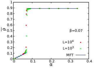
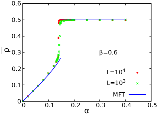
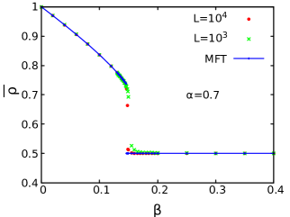
It is easy to see that these order parameters (IV.2)-(IV.4) reduce to the respective bulk density differences in an open TASEP with uniform hopping rates. The transitions would be second order if the respective order parameters defined above would vanish at the corresponding phase boundaries. Else, if instead they show discontinuities, the transitions are first order in nature. In this Section, we focus on the phase transitions in the restricted case with symmetric with a single minimum (as above). The more general cases including asymmetric will be discussed elsewhere in future. We use both MFT and MCS to analyse the phase transitions. We first study the LD-HD transition. To that end, we consider Eq. (III.7) or Eq. (III.16) for , and correspondingly Eq. (III.8) or Eq. (III.12) for . Since both , we conclude that the discriminant in each of Eq. (III.7) or Eq. (III.16) and Eq. (III.8) or Eq. (III.12), giving and at all . This in turn implies and necessarily. This holds even at the transition point making , which in turn means is finite at the transition. Thus the LD-HD transition in the MFT is first order, as in an open TASEP with constant hopping rates. We now turn to the LD-MC transition, which is a second order transition in an open TASEP with constant hopping. To analyse this for symmetric , we use the fact that (see above), and again consider Eq. (III.8) or Eq. (III.12) for . At the LD-MC transition . Since at any , the discriminant in Eq. (III.8) or Eq. (III.12) is generally positive except at discrete points where , which holds even at the LD-MC transition. Thus and hence at the transition point. Surprisingly, this means does not vanish at the transition, giving a first order transition here, in contrast to a second order LD-MC transition in an open TASEP with uniform hopping. Similar arguments can be used to show that in MFT, the HD-MC transition is also a first order transition, again in contrast to an open TASEP with uniform hopping. Thus, rather unexpectedly MFT predicts that all the three transitions are first order with a symmetric having one minimum. To verify these MFT predictions for our model numerically, we have studied the nature of the phase transitions numerically across the LD-HD, LD-MC and HD-MC phase boundaries. More specifically, we calculate:
(i) as a function of for a fixed , as approaches the LD-HD phase boundary; see Fig. 10(left) for a plot of the average density as a function of . On one side of the transition, is the mean LD phase density that rises with ; on the other side of it, is that remains independent of for a fixed . This plot clearly shows a jump in across the transition, meaning a first order transition, akin to an open TASEP with uniform hopping.
(ii) as a function of for a fixed , as approaches the LD-MC phase boundary; see Fig. 10(middle) for a plot of the average density as a function of . On one side of the transition, is the mean LD phase density that rises with ; on the other side of it, is that remains independent of as well as . Surprisingly, this plot clearly shows a jump in across the transition, meaning a first order transition, in contrast to an open TASEP with uniform hopping.
(iii) as a function of for a fixed , as approaches the HD-MC phase boundary; see Fig. 10(right) for a plot of the average density as a function of . On one side of the transition, is the mean HD phase density that decreases as increases; on the other side of it, is that remains independent of as well as . Surprisingly, this plot clearly shows a jump in across the transition, again implying a first order transition, again in contrast to an open TASEP with uniform hopping.
Our MCS studies show that in all these cases there is a jump in the density at the respective phase boundary, implying a discontinuous or a first order transition, in agreement with the MFT prediction for the same. This is a truly novel result, that shows how quenched disorder can alter the order of phase transitions. To benchmark our numerical codes, in Fig. 11 in Appendix A we have shown the analogous plots for the LD-HD, LD-MC and HD-MC transitions for an open TASEP with uniform hopping. Unsurprisingly. the plots in Fig. 11 show a first order LD-HD transition and second order LD-MC and HD-MC transitions, both in the MCS and MFT studies. That quenched disorder can change the order of transitions in pure models is well-known. For instance, Ref. prb shows that sufficiently strong quenched disorder can make the magnetic transition in ferromagnetic manganites first order. Similarly, quenched disorder can introduce a first order transition in the well-known Kuramoto model of oscillator synchronization kura . The current study forms yet another such example, and possibly the first of its kind in TASEP-like driven models with open boundary conditions.
V Summary and outlook
We have thus studied the totally asymmetric exclusion process with open boundaries having spatially smoothly varying hopping rates. Our study reveals the universal form of the phase diagrams for generic smooth hopping rates. Our results are sufficiently general and applies to any smoothly varying hopping rate functions. We construct the mean-field theory, and use that to outline a scheme to calculate steady state density profiles. Our method directly gives the steady state densities in terms of the current almost immediately by using the spatial constancy of the latter in the steady states. The different phases are then analysed by varying the boundary conditions in a straightforward manner. Unsurprisingly, the bulk steady state densities are generically space varying, unlike those in the conventional TASEP with uniform hopping (except along the special line ). These match well with those obtained from the MCS studies, lending credence to our mean-field analysis. Because of the spatially varying densities, the conventional way to characterise the phases via the densities, i.e., and in the bulk of the TASEP no longer holds. Rather one needs to resort to the equivalent conditions to decide the phases, since the current is a constant. This together with the condition that and everywhere in the bulk, allows us to distinguish the LD and HD phases. Further, the maximum steady state current that the system can sustain is no longer 1/4, but is , where is the minimum hopping rate. Surprisingly, our theory shows that the average bulk density in the MC phase can be more or less than 1/2, in direct contrast with conventional open TASEPs with uniform hopping. We show that the general effect of spatially varying hopping rates is to enlarge the MC region of the phase space, while shrinking the LD and HD regions. Furthermore, our work elucidates the universal phase diagram for various choices of the hopping rate function, highlighting the robustness of asymmetric exclusion process in an open system. Lastly but not the least, our MFT and MCS studies clearly show that both the LD-MC and HD-MC transitions in the model are first order for any symmetric hopping rate function having one minimum. This forms a truly novel outcome from this study. How this generalises to other forms of is an interesting question to be investigated in the future.
Our MFT scheme is sufficiently general. It applies for any that is smoothly and slowly varying. It would be interesting to extend our scheme to situations where is smooth and slowly varying in general, but can have a few finite discontinuities. This will be discussed in the future. It will also be important to study the effects of interactions in the systems arvind1 . In addition, there are in vivo situations, where is rapidly fluctuating in space dna , which breaks down the assumption of slowly varying . How an equivalent analysis may be carried out for such a system, and to what degree the present results may be valid there are interesting questions to study. Hydrodynamic approaches should be promising in this regards, which already provides initial clues to this problem erdmann ; see also Ref. astik-prr for a comprehensive hydrodynamics-based field theory approach to this problem in a closed geometry. It would also be interesting to apply the boundary layer theory developed in Ref. smb on our model, and determine the stationary densities and phases. We hope our work here will provide impetus to studies along these lines in future. Our results may be verified in model experiments on the collective motion of driven particles with light-induced activity light passing through a narrow channel. Spatial modulations of the hopping rate can be created by applying patterned or spatially varying illumination.
VI Acknowledgement
We thank S. Nag and A. Basu for helpful discussions. S.M. thanks SERB (DST), India for partial financial support through the CRG scheme [file: CRG/2021/001875].
Appendix A Phase transitions in an open TASEP with uniform hopping
We numerically study the LD-HD, LD-MC and HD-MC transitions. As expected, our studies show that the LD-HD transition is a first order transition, whereas the LD-MC and HD-MC transitions are second order in nature.
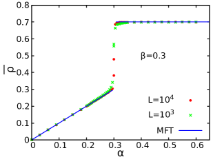
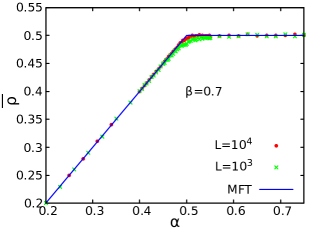
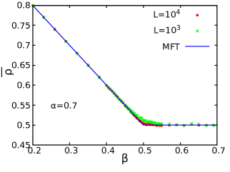
References
- (1) B. Schmittmann and R. Zia, in Phase Transitions and Critical Phenomena, edited by C. Domb and J. Lebowitz (Academic Press, London, 1995), Vol. 17.
- (2) B. Derrida and M. Evans, in Nonequilibrium Statistical Mechanics in One Dimension, edited by V. Privman (Cambridge University Press, Cambridge, UK, 1997), Chap. 14, pp. 277–304; G. Schütz, in Phase Transitions and Critical Phenomena, ed- ited by C. Domb and J. Lebowitz (Academic Press, San Diego, 2001), Vol. 19, pp. 3–251.
- (3) J. Krug, Phys. Rev. Lett. 67, 1882 (1991).
- (4) T. Chou, K. Mallick, and R. K. P. Zia, Rep. Prog. Phys. 74, 116601 (2011); S. E. Wells, E. Hillner, R. D. Vale, and A. B. Sachs, Mol. Cell 2, 135 (1998); S. Wang, K. S. Browning, and W. A. Miller, EMBO J. 16, 4107 (1997); Z. A. Afonina et al., Nucleic Acids Res. 42, 9461 (2014); D. W. Rogers et al., PLoS Comput. Biol. 13, e1005592 (2017).
- (5) C. Richer and S. Hasiak, Town Planning Review 85, 217 (2014).
- (6) R. J. Harris and R. B. Stinchcombe, Phys. Rev. E 70, 016108 (2004); G. Lakatos, J. O’Brien and T. Chou, J. Phys. A: Math. Gen. 39, 2253 (2006); R. B. Stinchcombe and S. L. A. de Queiroz, Phys. Rev. E 83, 061113 (2011).
- (7) G. Tripathy and M. Barma, Phys. Rev. E 58, 1911 (1998); M. Bengrine, A. Benyoussef, H. Ez-Zahraouy, and F. Mhirech, Phys. Lett. A 253, 135 (1999); C. Enaud and B. Derrida, Europhys. Lett. 66, 83 (2004); L. B. Shaw, J. P. Sethna, and K. H. Lee, Phys. Rev. E 70, 021901 (2004).
- (8) T. Banerjee and A. Basu, Phys. Rev. Research 2, 013025 (2020).
- (9) A. Haldar, A. Basu, Phys Rev Research 2, 043073 (2020).
- (10) D. D. Erdmann-Pham, K. D. Duc, and Y. S. Song, Cell systems 10, 183 (2020).
- (11) R. A. Blythe and M. R. Evans, J. Phys. A: Math. Theo. 40, R333 (2007).
- (12) A. Parmeggiani, T. Franosch, and E. Frey, Phys. Rev. E 70, 046101 (2004).
- (13) N. Sarkar and A. Basu, Phys. Rev. E 90, 022109 (2014).
- (14) T. Banerjee, A. K. Chandra, and A. Basu, Phys. Rev. E 92, 022121 (2015).
- (15) B. Pal and A. K. Gupta, J. Phys. A: Math. Theor. 54, 025005 (2020).
- (16) A. Jindal, T. Midha and A. K. Gupta, J. Phys. A: Math. Theor. 53 235001 (2020).
- (17) J. Krug, Braz. J. Phys. 30, 97 (2000).
- (18) T. Reichenbach, T. Franosch, and E. Frey Eur. Phys. J. E 27, 47 (2008).
- (19) This would be strictly true if due to the symmetry of . Even when in the MC phase, holds to a high accuracy, as can be seen from our MCS study results. This is presumably due to the fact the affects for all practical purposes only the boundary layers.
- (20) J. Salafranca and L. Brey, Phys. Rev. B 73, 214404 (2006).
- (21) H. Hong and E. A. Martens, arXiv: 2111.0893.
- (22) B. Alberts, A. Johnson, J. Lewis, M. Raff, K. Roberts, and P. Walter, Molecular Biology of the Cell, 4th ed. (Garland Science, 2002); B. Li, M. Carey, and J. L. Workman, Cell 128, 707 (2007); C. Y. Lin, J. Lovén, P. B. Rahl, R. M. Paranal, C. B. Burge, J. E. Bradner, T. I. Lee, and R. A. Young, ibid. 151, 56 (2012); J. L. Workman and R. E. Kingston, Annu. Rev. Biochem. 67, 545 (1998).
- (23) S. Mukerjee and S. M. Bhattacharjee, J. Phys. A: Math. Gen. 38, L285 (2005); S. Mukherji and V. Mishra, Phys. Rev. E 74, 011116 (2006); S. M. Bhattacharjee, J. Phys. A: Math. Theor. 40, 1703 (2007); S. Mukherji, Phys. Rev. E 79, 041140 (2009); , 83, 031129 (2011); A. K. Gupta and I. Dhiman, ibid. 89, 022131 (2014); S. Mukherjee and S. M. Bhattacharjee, Sci. Rep. 9, 5697 (2019).
- (24) See, e.g., I. Buttinoni et al., J. Phys.: Condens. Matter 24, 284129 (2012).