On the explosive phase of the tearing mode in double current sheet plasmas: effect of the equilibrium magnetic configuration on the onset threshold and growth rate

Abstract

Magnetic reconnection associated with the tearing instability occurring in double-current sheet systems is investigated within the framework of reduced resistive magnetohydrodynamics (MHD) in a two-dimensional Cartesian geometry. The explosive non linear phase is particularly explored using the adaptive finite-element FINMHD code. The critical aspect ratio, that is defined as the minimum $L/x_{s}$ ratio (with $L$ and $x_{s}$ being the periodic system length and half-distance between the two current layers respectively) necessary for non linear destabilization after the linear and early non linear saturation phases, is obtained. The latter threshold is independent of the details of the chosen initial equilibrium (double Harris-like magnetic profile) and of the resistivity. Its value is shown to be $4.7$, that is close and slightly smaller than the value of order $5$ deduced using a more particular equilibrium configuration in previous studies. The time dependence of the kinetic energy ($E_{K}$) is shown to follow a double exponential law, $E_{K}\propto\exp\ [e^{(\gamma^{*}t)}]$, with a pseudo-growth rate $\gamma^{*}\simeq 0.1\ t_{A}^{-1}$ ($t_{A}$ being the characteristic Alfvén time) that is again independent of the configuration and resistivity. The mechanism offers a possible explanation for the sudden onset of explosive magnetic energy release occurring on the fast Alfvén time scale in disruptive events of astrophysical plasmas with pre-existing double current sheets like in the solar corona.

1 Introduction

The tearing mode developing in current sheet plasmas is believed to play a significant role during explosive phenomena observed in different magnetized astrophysical systems like the solar corona, the solar wind, or pulsar winds. When a single electric current sheet (corresponding to a magnetic reversal) is present, the tearing instability is considered to be a slow mode as it involves a magnetic reconnection process in the form of magnetic islands growing on a resistive time scale (except if plasmoid chains are able to develop in cases of very long and thin layers). The tearing mode of such highly conducting plasmas under consideration in this study has been extensively investigated in planar and sheet pinch configurations (Priest & Forbes, 2000). The latter magnetohydrodynamic (MHD) instability is characterized by a threshold for the wavenumber $k$, as $k\leq k_{M}$ is required. The maximum wavenumber $k_{M}$ depends on the details of the equilibrium profile, and its value is $k_{M}=1/a$ for the standard Harris profile, where $a$ defines the half-thickness of the current sheet. This linear stability threshold can be easily translated into a condition $L\geq L_{min}$ for the length of the system, where $L_{min}=2\pi/k_{M}$ (Biskamp, 2009). These resistive instabilities are admitted to grow on a characteristic time scaling as $S^{1/3}-S^{3/5}$, where $S$ is the Lundquist number defined as $S=aV_{A}/\eta$ (with $V_{A}$ and $\eta$ being the Alfvén velocity and the small magnetic diffusivity parameter respectively). For example, as the typical $S$ value for the solar coronal plasma is $\sim 10^{10}$, the characteristic tearing time scale cannot account for fast time scales involved in solar flares by many orders of magnitude (i.e. a few years/months versus a few minutes).

On another hand, multiple current sheets due to many field reversals are also expected to form in such plasmas, giving rise to multiple tearing instabilities. A richer dynamics is thus expected with a multi-regime feature for the reconnection process and associated magnetic energy release, that is not observed for a single current sheet. This is the case for a double current sheet system. Interestingly, for this latter configuration, an explosive growth phase can be obtained in association with the so called double tearing mode (DTM hereafter). Indeed, after a long-time-scale evolution of slow resistive linear growth (similar to the growth of a single tearing mode with similar scaling laws) followed by a phase of saturation, the DTM suddenly changes to rapid growth (Ishii et al., 2002; Wang et al., 2007; Janvier et al., 2011; Zhang & Ma, 2011; Akramov & Baty, 2017). During this explosive phase, the kinetic energy associated to the flow can increase by several orders of magnitude in a few Alfvén times quasi-independently of the resistivity $\eta$ or Lundquist number $S$. Extensive studies using the simplest MHD framework (i.e. reduced MHD equations in a two-dimensional planar geometry) have shown that the explosive phase is triggered by a structure-driven non linear instability (Ishii et al., 2002; Janvier et al., 2011). The onset of this ideal MHD instability is ascribed to a critical deformation of the magnetic islands growing on the two current layers. The explosive reconnection is triggered only when the aspect ratio $L/x_{s}$ (with $L$ and $x_{s}$ being the periodic system length and the half-distance between the two current layers respectively) is higher than a critical value, that is $\simeq 5$, independently of the resistvity. Otherwise the system with the two magnetic islands no longer evolves. This second critical length value $L_{c}$ is in general higher than the $L_{min}$ one.

However, the previously cited studies have mostly employed a particular magnetic field profile for the initially unstable equilibrium, which is generally assumed in the context of laboratory plasmas. The scope of the present study is precisely to test the robustness of this critical aspect ratio value by employing another profile which is the generalization of a Harris-type profile generally used for tearing mode of a single current sheet. Moreover, our profile parametrization allows to study the effect of the shear parameter (deduced from the thickness of the two current layers at the reversal location of the magnetic field), independently of the distance between the two layers $2x_{s}$. Finally, we investigate how the fast Alfvénic time scale (previously reported) for the non linear growth depends on the initial equilibrium and also from the ’distance’ to the non linear threshold. We use a strongly adaptive finite-element code, FINMHD, that has been specifically designed to address such reconnection problem within the framework of reduced resistive MHD in a two-dimensional Cartesian geometry. The outline of the paper is as follows. In Section 2, we briefly present the code and the initial setup. Section 3 is devoted to the presentation of the results. Finally, we conclude in section 4.

2 FINMHD code and initial setup

The usual set of reduced MHD equations in two dimensions (2D) (i.e. $x-y$ plane) is considered to be a good approximation to represent the dynamics in a plane perpendicular to a dominant and constant magnetic field component ($B_{z}$). In this way, the incompressibility assumption in the 2D plane is admitted to be well justified. Instead of taking a standard formulation in terms of perpendicular velocity and magnetic vectors ($\bm{V}$ and $\bm{B}$ respectively), it is generally advantageous to use another formulation with scalar variables like stream functions (hereafter $\phi$, and $\psi$), as this ensures the divergence-free property for these two vectors. Moreover, in order to facilitate the numerical implementation, a (dimensionless) model using the electric current density $J$ and the flow vorticity $\omega$ for the main variables is adopted in FINMHD (Baty, 2019),

$$\frac{\partial\omega}{\partial t}+(\bm{V}\cdot\bm{\nabla})\omega=(\bm{B}\cdot\bm{\nabla})J+\nu\bm{\nabla}^{2}\omega,$$ (1)

$$\frac{\partial J}{\partial t}+(\bm{V}\cdot\bm{\nabla})J=(\bm{B}\cdot\bm{\nabla})\omega+\eta\bm{\nabla}^{2}(J-J_{e})+g(\phi,\psi),$$ (2)

$$\bm{\nabla}^{2}\phi=-\omega,$$ (3)

$$\bm{\nabla}^{2}\psi=-J,$$ (4)

with $g(\phi,\psi)=2\left[\frac{\partial^{2}\phi}{\partial x\partial y}\left(\frac{\partial^{2}\psi}{\partial x^{2}}-\frac{\partial^{2}\psi}{\partial y^{2}}\right)-\frac{\partial^{2}\psi}{\partial x\partial y}\left(\frac{\partial^{2}\phi}{\partial x^{2}}-\frac{\partial^{2}\phi}{\partial y^{2}}\right)\right]$. We have introduced the two stream functions, $\phi(x,y)$ and $\psi(x,y)$, defined as $\bm{V}={\nabla}\phi\wedge\bm{e_{z}}$ and $\bm{B}={\nabla}\psi\wedge\bm{e_{z}}$ ($\bm{e_{z}}$ being the unit vector perpendicular to the $xOy$ simulation plane). Note that $J$ and $\omega$ are the $z$ components of the current density and vorticity vectors, as $\bm{J}=\nabla\wedge\bm{B}$ and $\bm{\omega}=\nabla\wedge\bm{V}$ respectively (with units using $\mu_{0}=1$). Note also that we consider the resistive diffusion via the $\eta\bm{\nabla}^{2}J$ term ($\eta$ being the resistivity assumed uniform for simplicity), and also a viscous term $\nu\bm{\nabla}^{2}\omega$ in a similar way (with $\nu$ being the viscosity parameter). The above definitions results from the choice $\psi\equiv A_{z}$, where $A_{z}$ is the $z$ component of the potentiel vector $\bm{A}$ (as $\bm{B}=\nabla\wedge\bm{A}$). FINMHD code is based on a finite element method using triangles with quadratic basis functions on an unstructured grid. A characteristic-Galerkin scheme is chosen in order to discretize in a stable way the Lagrangian derivatives appearing in the two first equation. Moreover, a highly adaptive (in space and time) scheme is developed in order to follow the rapid evolution of the solution, using either a first-order time integrator (linearly unconditionally stable) or a second-order one (subject to a CFL time-step restriction). Typically, a new adapted grid can be computed at each time step, by searching the grid that renders an estimated error nearly uniform. More precisely, the method allows to always cover the current structures with a few tens of triangles at any time, by using the Hessian matrix of the current density as the main refinement parameter. The technique used in FINMHD has been tested on challenging tests, involving unsteady strongly anisotropic solution for the advection equation, formation of shock structures for viscous Burgers equation, and magnetic reconnection for the reduced set of MHD equations. The reader should refer to Baty (2019) for more details on the numerical scheme and also to the following references for applications to different aspects of magnetic reconnection in MHD framework (Baty, 2020a, b, c).

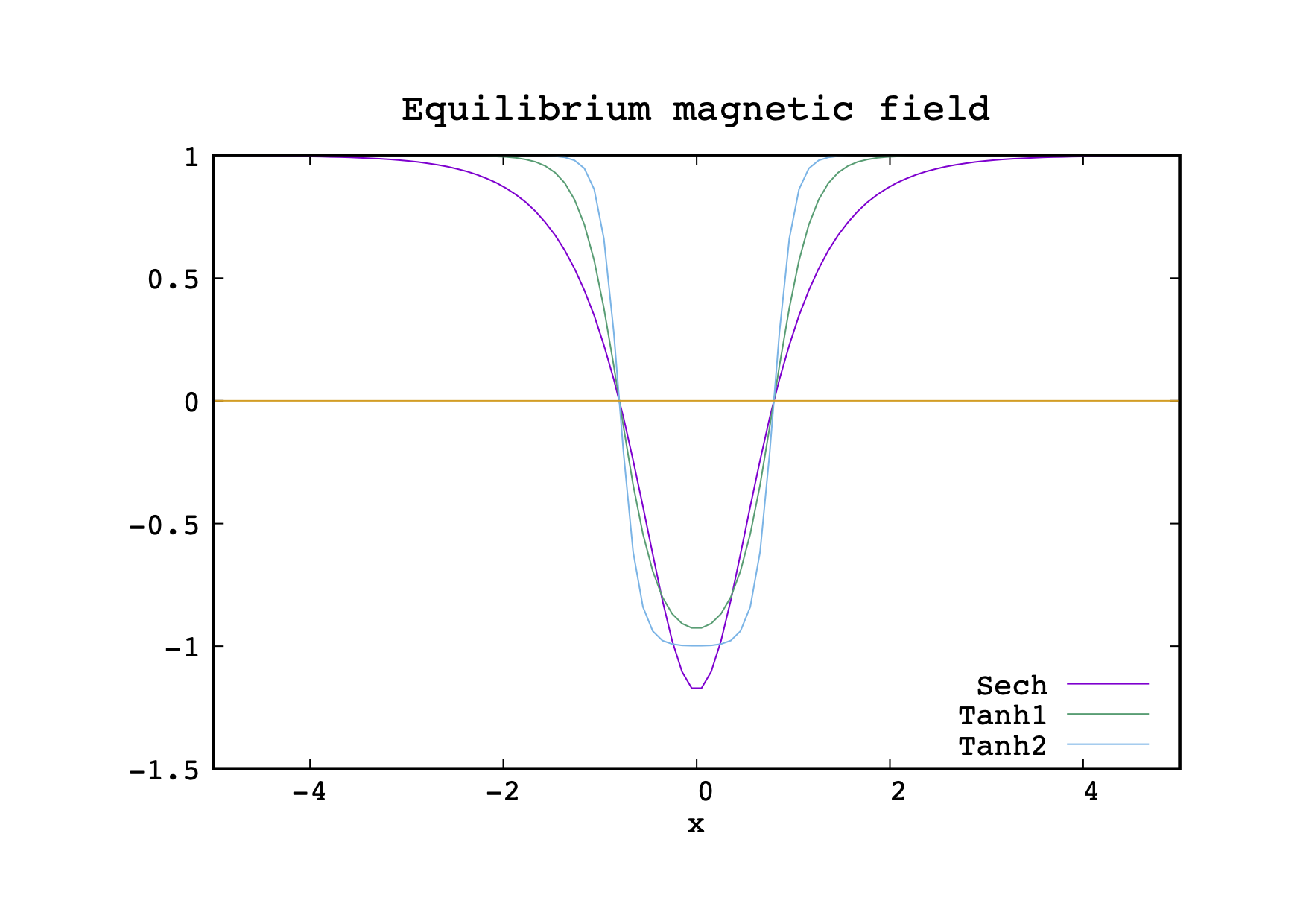
Figure 1: Initial configuration for the equilibrium magnetic field $B_{e}(x)/B_{0}$ for the ’sech’ profile and for two Harris-like ’tanh’ profiles (using $a=0.2$ for ’tanh2’, and $a=0.4$ for ’tanh1’). The field reversals (intersection with horizontal line) are situated at $x=\pm x_{s}=\pm 0.8$ for the different equilibria.

An initial one dimensional equilibrium is considered by taking an analytical expression for the $y$ component of the magnetic field profile $B_{y}=B_{e}(x)$. In the present work, a double Harris-like profile (quoted as ’tanh’ below) is assumed,

$$B_{e}(x)=B_{0}\left[1+\tanh\left(\frac{x-x_{s}}{a}\right)-\tanh\left(\frac{x+x_{s}}{a}\right)\right],$$ (5)

with two hyperbolic tangent-like reversals at $x=\pm x_{s}$, a magnetic shear defined by the length scale $a$, and an asymptotic magnetic field amplitude $B_{0}$ at large distance. The corresponding current density is,

$$J_{e}(x)=\frac{B_{0}}{a}\left[\frac{1}{\cosh^{2}[(x-x_{s})/a]}-\frac{1}{\cosh^{2}[(x+x_{s})/a]}\right],$$ (6)

which is also used in Equation (2) in order prevent the diffusion of the ideal equilibrium via the $-\eta\bm{\nabla}^{2}J_{e}$ source term. Indeed, such diffusion is unwanted when the resistivity parameter is not small enough. Moreover, a true ideal MHD equilibrium should require a thermal pressure term $P(x)$ or a $x$ dependence for a perpendicular magnetic field component (i.e. $B_{z}(x)$ not included in our model) in order to ensure the equality, $\bm{J}\times\bm{B}-\nabla P=0$ in the momentum MHD equation. However, working with the vorticity equation only requires $\bm{B_{e}}\cdot\bm{\nabla}J_{e}$ to vanish, which is automatically satisfied (see Equation 1).

In most previous studies (see Janvier et al. (2011) for example), another equilibrium magnetic field configuration (quoted as ’sech’ below) was applied as,

$$B_{e}(x)=B_{0}\left[1-(1+b_{c})\operatorname{sech}(\zeta x)\right],$$ (7)

where the parameters $b_{c}$ and $\zeta$ are chosen in such a way to set the reversal locations at $x_{s}$ via $\operatorname{sech}(\zeta x_{s})=1/(1+b_{c})$, the local magnetic shear being equal to $\pi/2$. For example, values of $b_{c}=1.18$ and $\zeta=1.77$ were used for an equilibrium with $x_{s}=0.8$, which is plotted in Figure 1. One can also compare the latter profile with our ’tanh’ equilibria using two different magnetic shear values, i.e. for current layer half-thickness $a=0.2$ and $a=0.4$.

3 Results

In order to have an overview of the scenario leading to the explosive phase during the DTM evolution, we present below the results of a representative case of an unstable ’tanh’ equilibrium profile with $x_{s}=0.8$ and $a=0.3$. The periodic longitudinal length value is chosen to be $L=4$. In this case, one can first check that DTM mode is linearly unstable as the corresponding maximum normalized number $ka=2\pi a/L\simeq 0.47$ is indeed lower than unity. Equivalently, the length value $L$ is higher than the critical minimum value, $L_{min}$, for linear destabilization of the DTM for the chosen ’tanh’ equilibrium profile, that is $L_{min}\simeq 1.88$. The chosen resistivity parameter is $\eta=10^{-3}$, and the magnetic Prandtl number is $P_{r}=\nu/\eta=1/3$. In this work, we consider the low viscosity regime in order to compare to previous works where a zero viscosity was adopted (Janvier et al., 2011).

Note also that, we choose $B_{0}=1$ defining thus our normalization. Consequently, the time variable $t$ is normalized using the Alfvén time $t_{A}=l/V_{A}$, where $l$ is the unit distance and $V_{A}$ is the Alfvén velocity based on $B_{0}$ (i.e. $V_{A}=1$). In this work, the simulation domain is situated in the $x$-range $[-L_{x}/2:L_{x}/2]$ with $L_{x}=4$ corresponding to an outer boundary placed sufficiently far enough away in order to not influence the main dynamics. Fixed boundary conditions are imposed at $x=\pm L_{x}/2$. Periodic boundary conditions are assumed in the $y$ direction in order to select different $k_{m}$ wavenumber values according to $k_{m}=2\pi m/L$ ($m$ being an integer) for a given $L_{y}=L$ value. The linearly fastest DTM instability in this work corresponds to a $m=1$ mode, thus involving a single $m=1$ magnetic island growing on each current layer (see below).

For this representative case, as a result of the adaptive refinement strategy, the minimum reached edge size of the triangles during the simulation varies between $h_{min}\simeq 0.01$ (necessary to resolve the equilibrium structure at very early times) and $h_{min}\simeq 0.001$ (necessary to resolve intense localized secondary current layers during strongly non linear phase). The imposed maximum edge size is $h_{max}\simeq 0.1$ mainly covering regions where the current density is very low. The corresponding total number of triangles varies between $15000$ and $35000$ approximately. One must note that, a higher number of triangles with a smaller minimum edge size is consequently required when a smaller resistivity is employed.

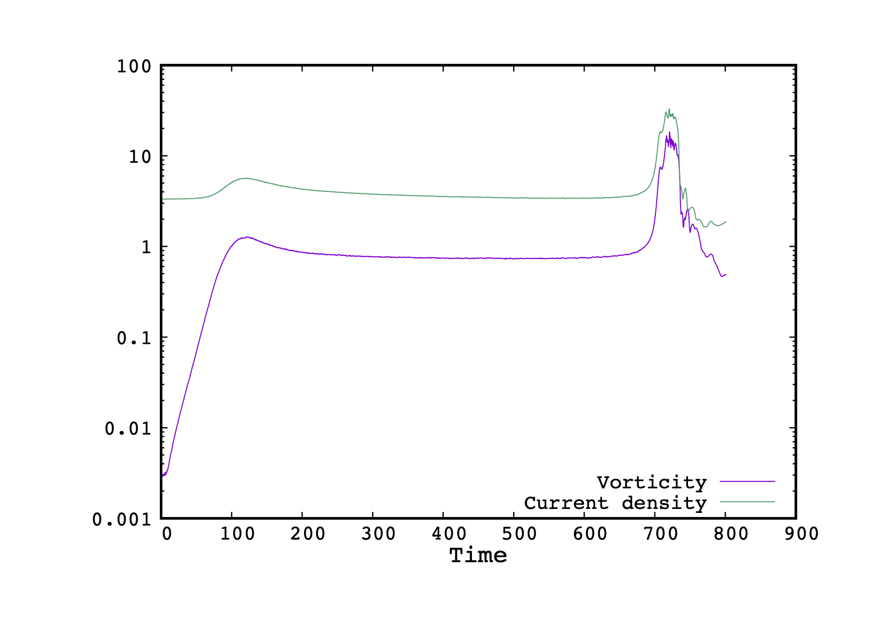
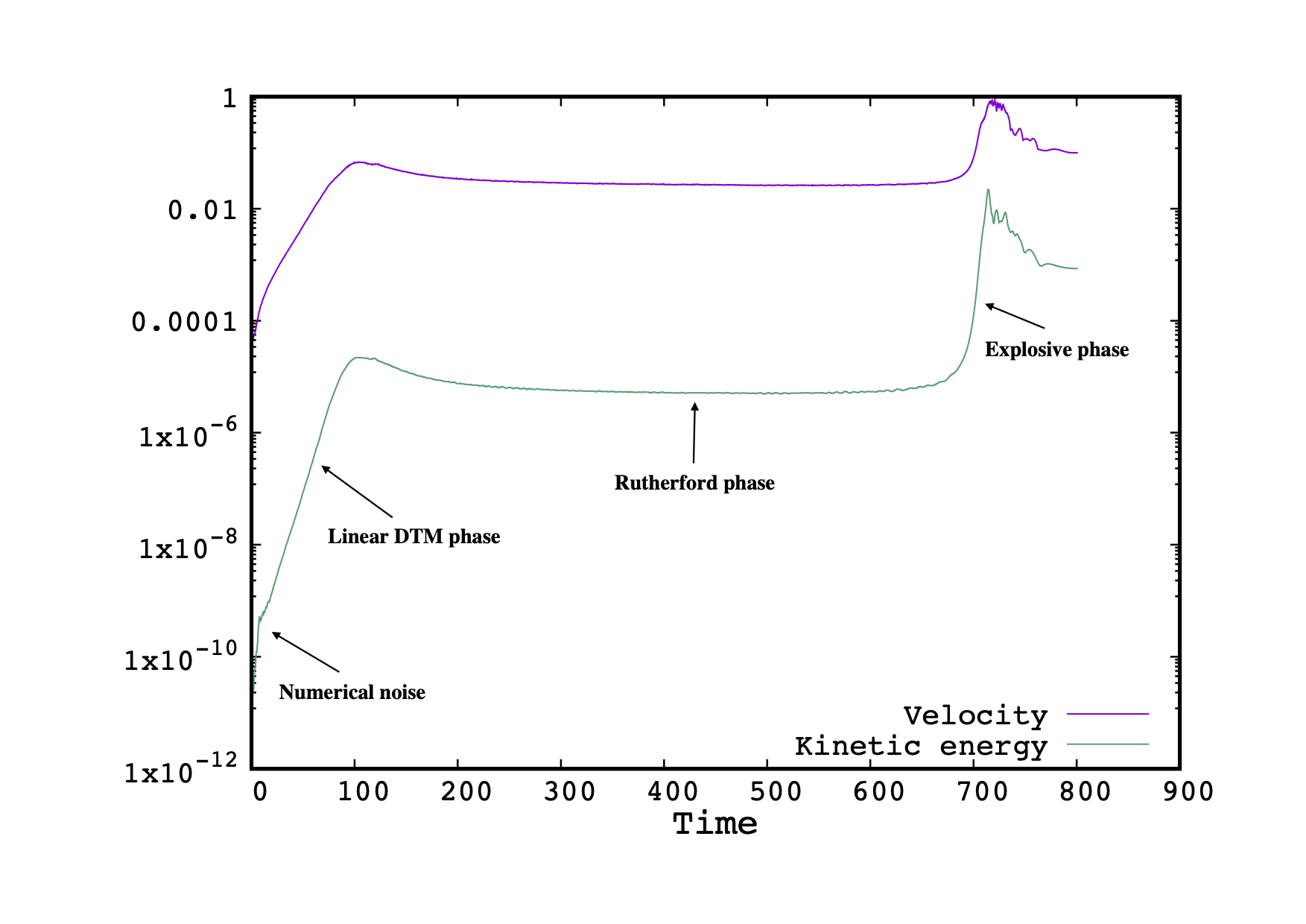
Figure 2: (Left panel) Time evolution of the maximum vorticity $\omega_{M}$ and associated maximum current density $J_{M}$ for a case exhibiting an explosive non linear evolution at $t\simeq 700$ , and (right panel) corresponding time evolution of the maximum velocity ($V_{y}$ component) and kinetic energy $E_{k}$ (right panel). The time is expressed in Alfvén time unit $t_{A}$ (see text).

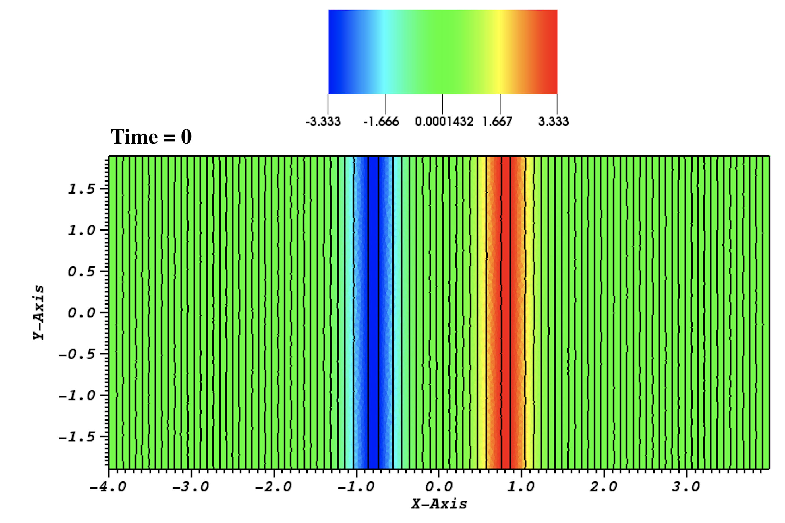
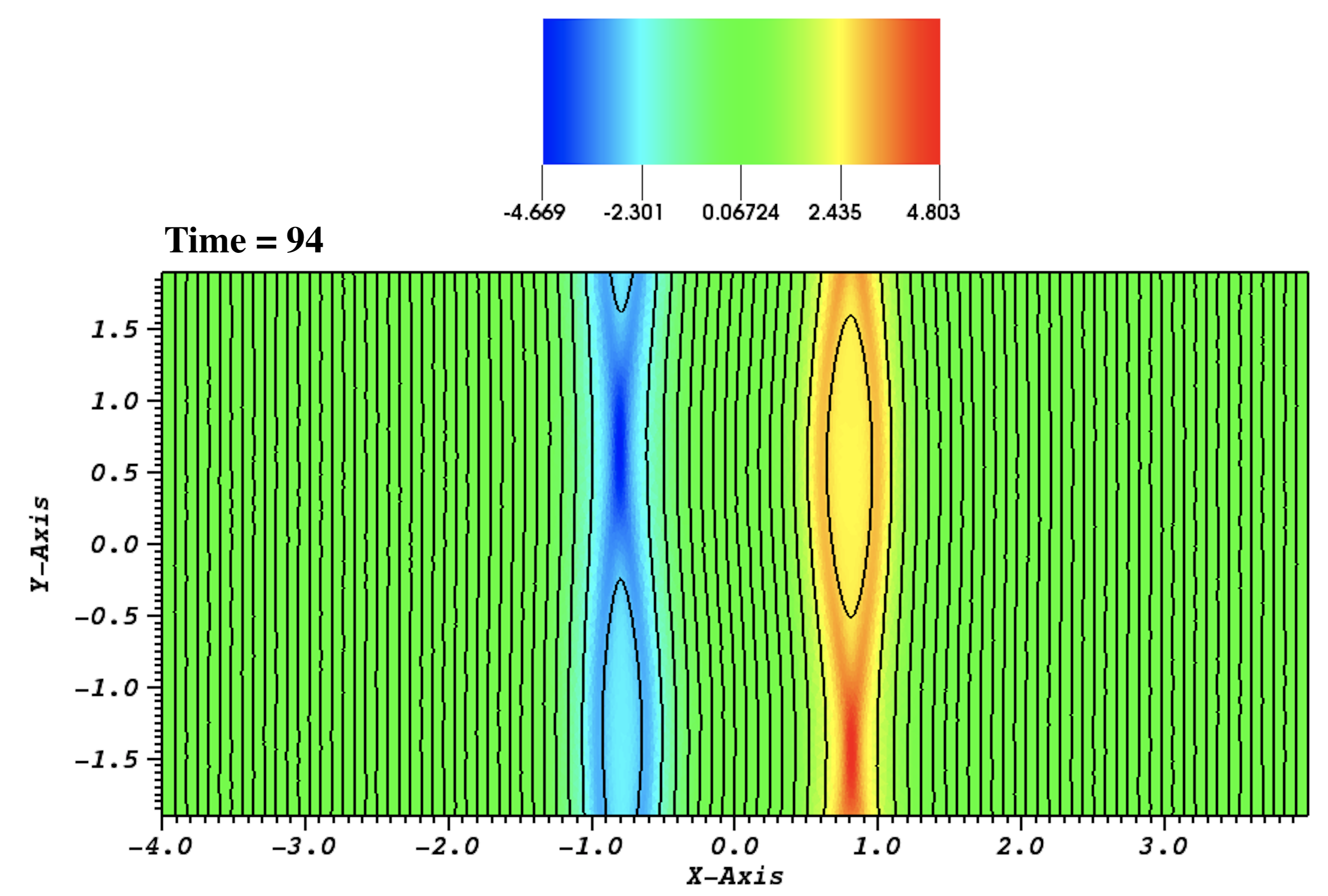
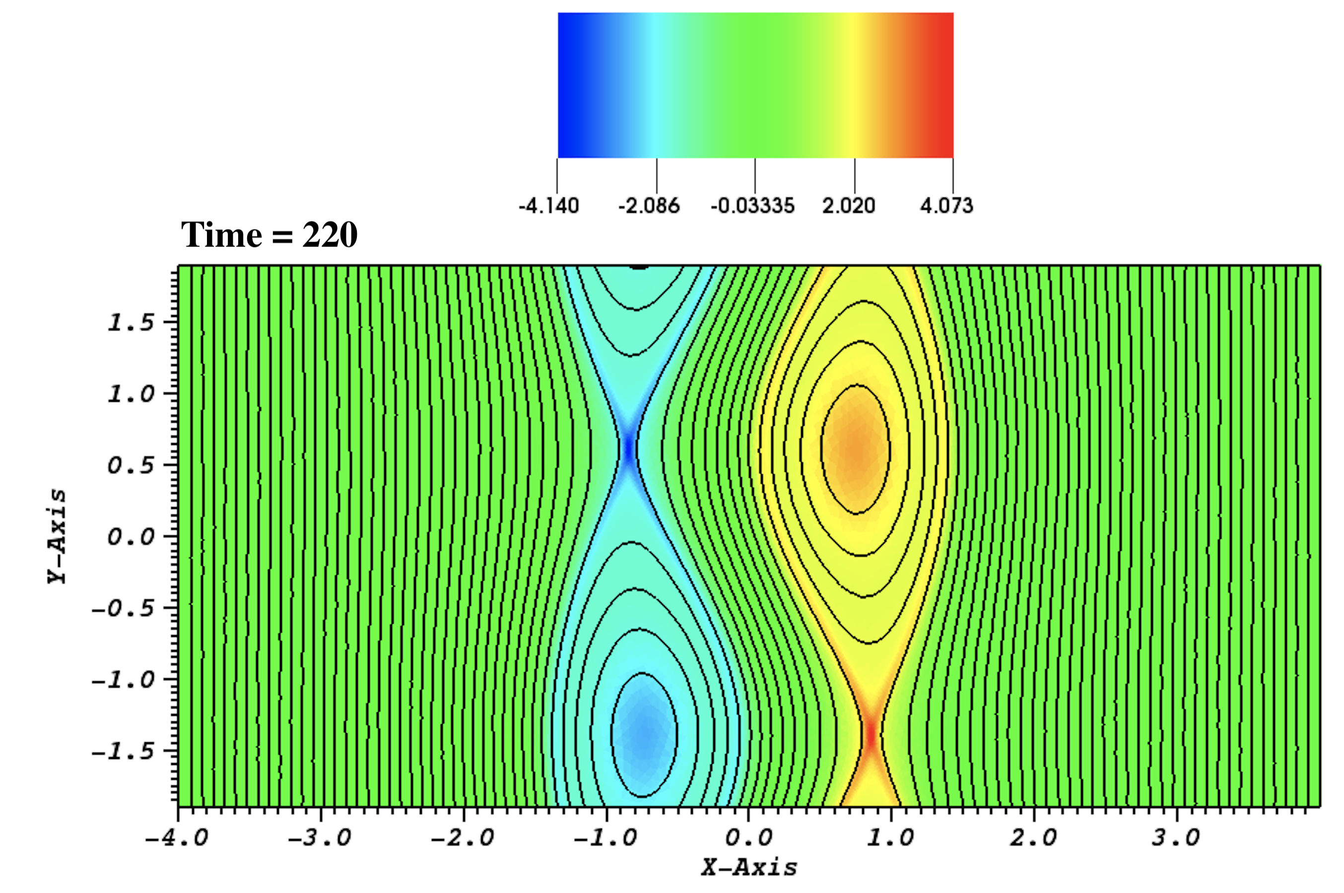
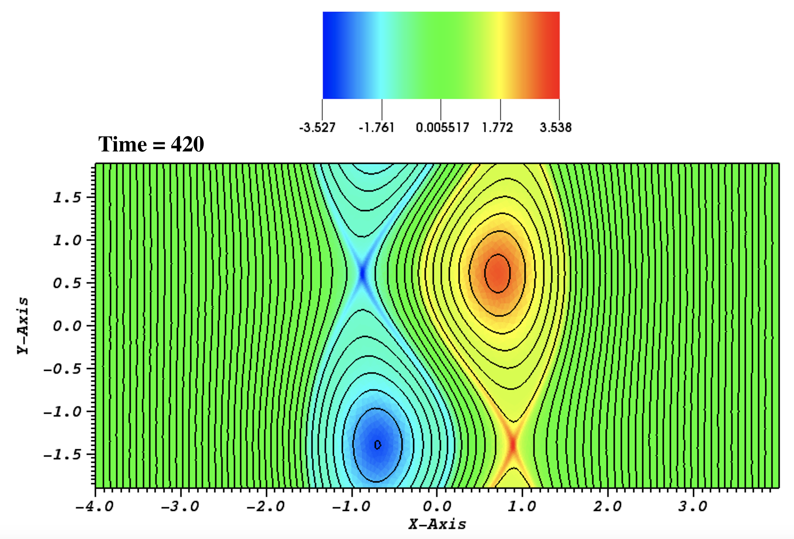
Figure 3: Colored iso-contour map of the current density at different selected times during the representative simulation case of previous figure (see also text), overlaid with corresponding selected magnetic field lines. Only early times corresponding to the two first phases are taken.

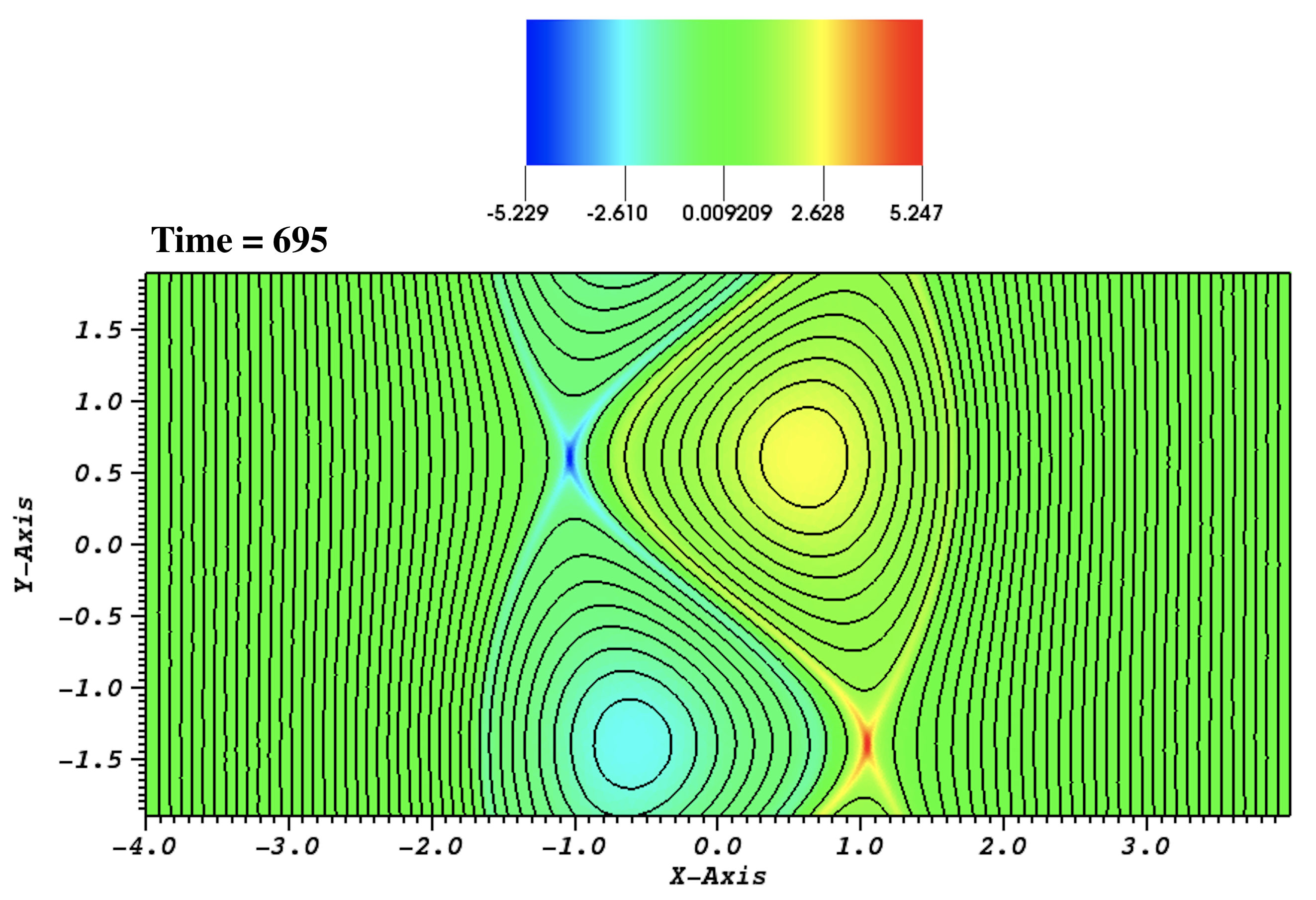
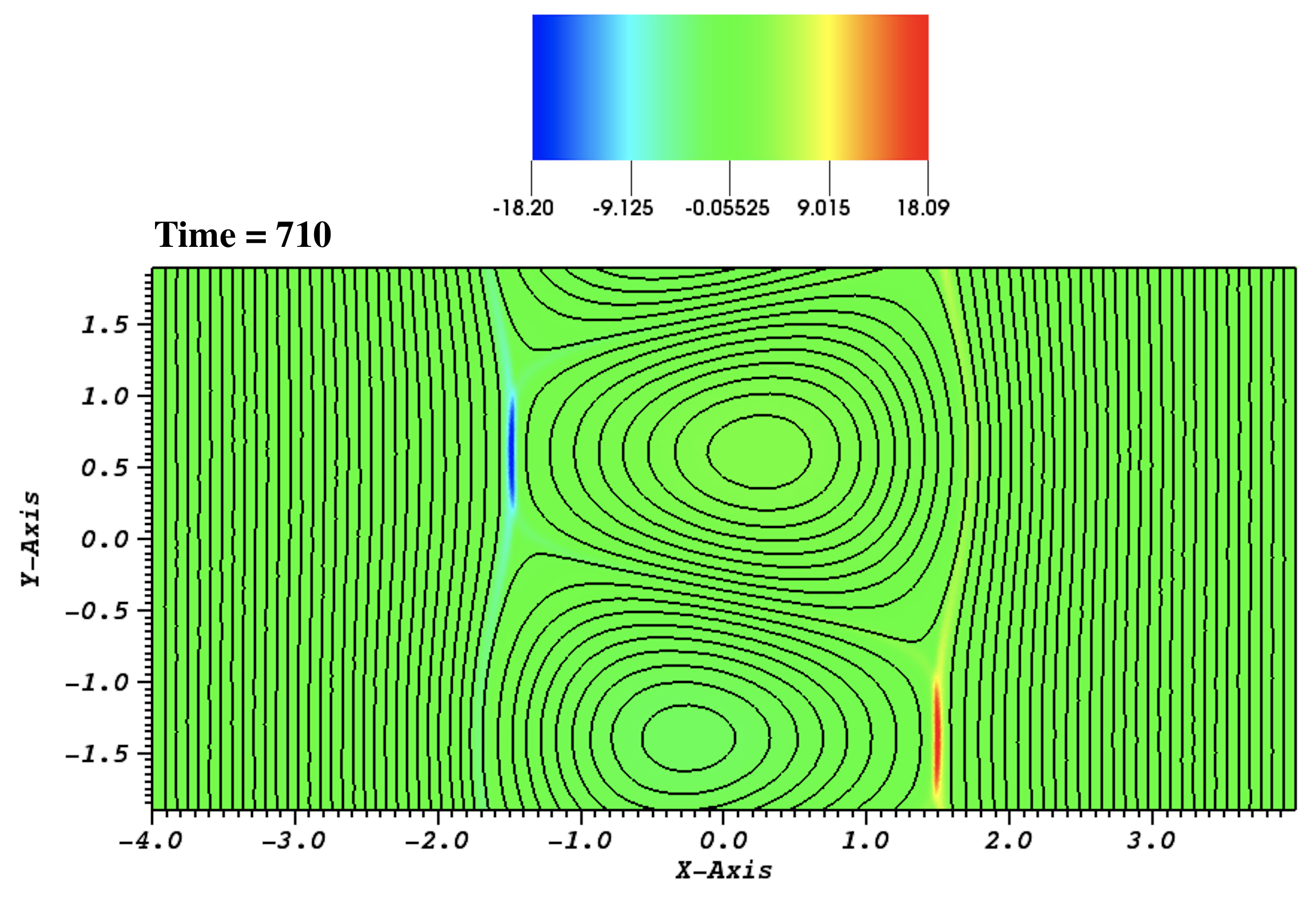
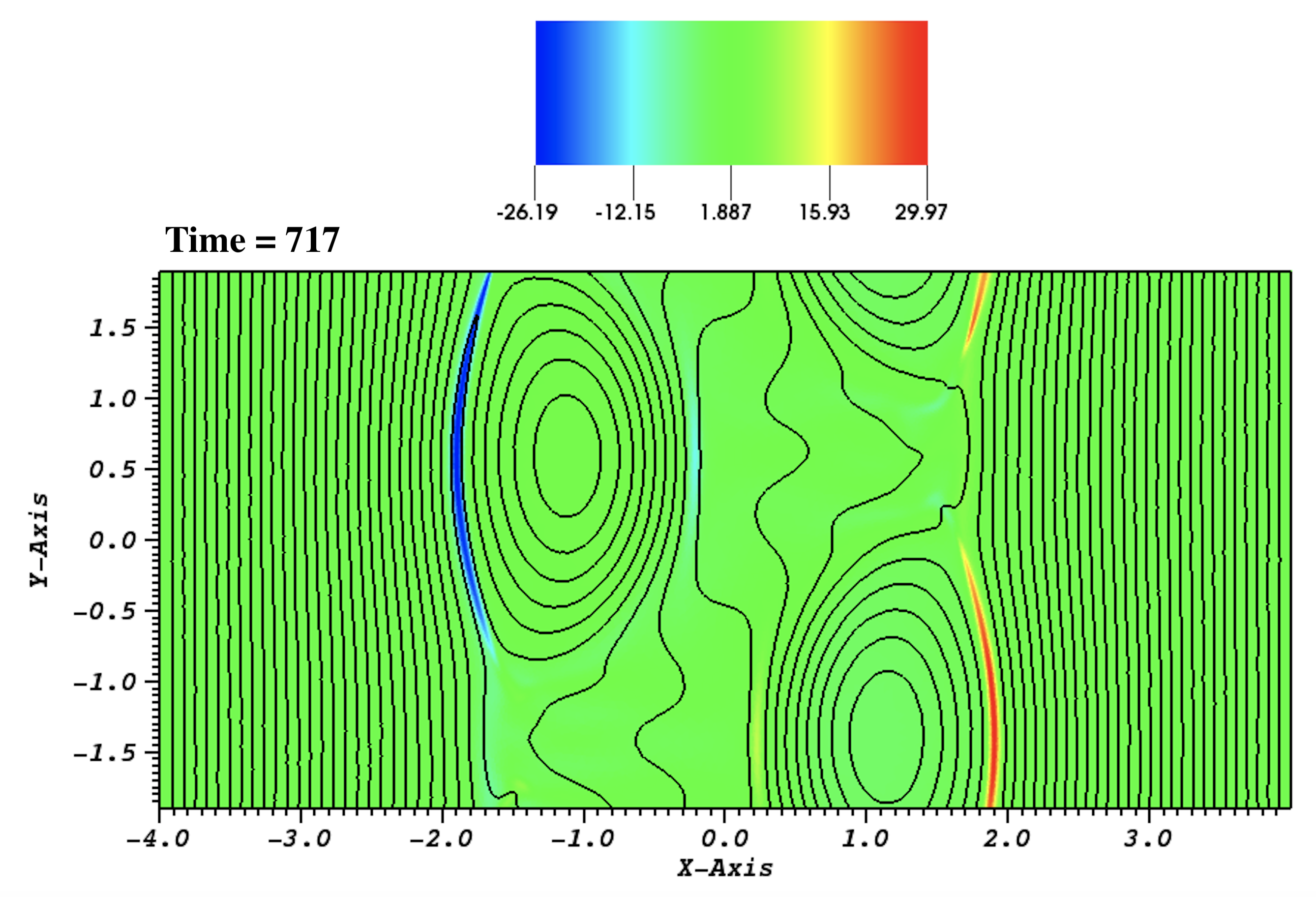
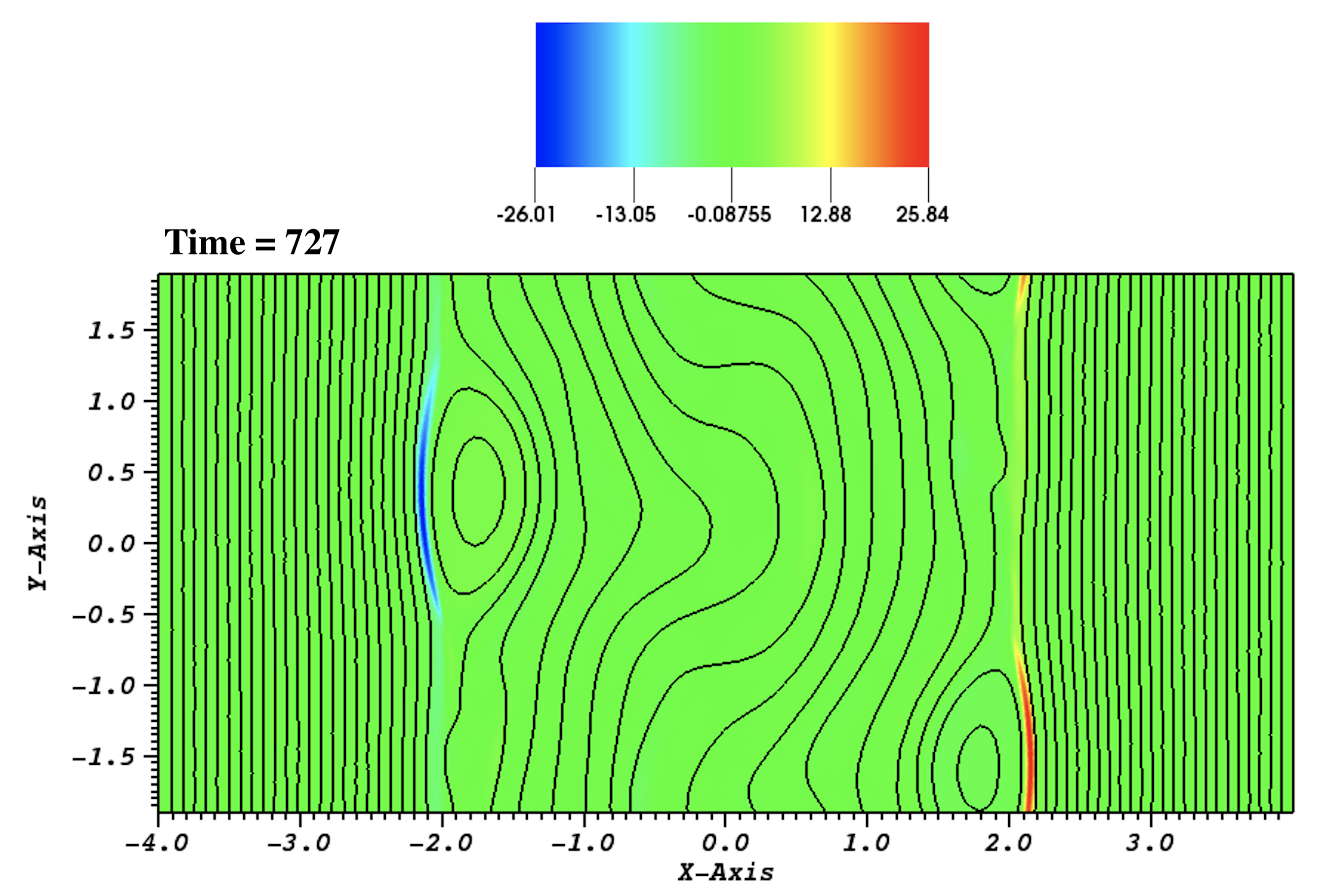
Figure 4: Same as previous figure for later times $t\lower 2.15277pt\hbox{$\;\buildrel>\over{\sim}\;$}700$ focusing on the explosive phase.

3.1 Overview of the explosive DTM dynamics

Figure 2 (left panel) shows the time evolution of the maximum vorticity $\omega_{M}$ and of the maximum current density $J_{M}$ measured over the whole computational domain, whilst the corresponding maximum velocity amplitude ($V_{y}$ component) and the integrated kinetic energy $E_{K}$ are plotted in right panel. At early time, after a short period of oscillating numerical noise (that is barely visible in $E_{K}$ curve for example), one can clearly see for $t\lower 2.15277pt\hbox{$\;\buildrel<\over{\sim}\;$}100$ the linear development of the DTM exhibiting a linear dependence with time (in our semi-log representation) for $\omega_{M}$, $V_{y}$, and $E_{K}$. The slope measured for $E_{K}$ is obviously twice the slope for $V_{y}$ or $\omega_{M}$, and represents the linear growth rate. More precisely, one can deduce the linear growth rate $\gamma_{l}$ of the DTM instability, as $\gamma_{l}=\partial_{t}E_{K}/E_{K}$. Note that $\gamma_{l}\propto\eta^{3/5}\propto S^{-3/5}$ for such resistive instability (Biskamp, 2009). Figure 3 illustrates the spatial structure associated to the deformation of the current density and resulting magnetic field topology at different times. As expected, the DTM is characterized by two magnetic islands growing on the two initial current layers. Moreover, the corresponding observed eigenmode appears to be anti-symmetric, with an out-of-phase island structure between the two current layers. Indeed, the $O$-point of the magnetic island at one current sheet is facing with the $X$-point of the island at the other current sheet. As shown from linear stability analysis, this type of anti-symmetric mode, called A-mode (Wei et al., 2020), is expected to dominate the second type of mode (symmetric one) called S-mode.

The linear phase is followed by a saturation called a Rutherford regime, that has been extensively studied for single tearing modes. In this regime, $E_{K}$ remains quasi-steady, but the perturbed magnetic energy (not shown) continues to grow algebraically (see Janvier et al. (2011) and references therein) as the flow and magnetic flux are decoupled. This second phase exhibits a rather long evolution (at least for the parameters chosen in this case) with the two islands growing on a pure resistive time scale (see for example the snapshots at $t=220$ and $t=420$ in Figure 3).

After this Rutherford phase, an abrupt growth in all the physical variables is observed at $t\sim 700$ in Figure 2. The corresponding contour plot of the current density overlaid with magnetic field lines (in Figure 4) show that this third phase begins with a sudden triangular deformation of the islands (snapshot at $t=695$). This is followed by an increase of the current density at the two $X$-points (see snapshot at $t=710$), which drives a second phase of magnetic reconnection, ending when all the closed field lines situated inside the magnetic islands have reconnected with the external ones (i.e. at $t\simeq 730$). The final state at the end of the simulation tends to be a relaxed configuration free of magnetic islands and current layers, and the corresponding magnetic field lines tend to become straight again.

Note that, the process of magnetic reconnection during the latter phase is inverse when compared to the one associated to the linear DTM, as the closed field lines where forming during islands linear growth instead of disappearing during the explosive phase. The mechanism at the origin of this explosive reconnection dynamics was identified as a structure-driven instability, with a threshold ascribed to a critical magnetic island deformation (Janvier et al., 2011). In summary, it is shown that the nonlinear destabilization is obtained only when the ratio $L/x_{s}$ is higher than a value of order $5$ (see Figure 2 in Janvier et al. (2011)) for the ’sech’ profile. Here, we have used a case for the ’tanh’ profile having exactly this critical ratio, as $L/x_{s}=5$ for this illustrative case.

So, let us now investigate the existence/dependence of this critical aspect ratio value on the initial magnetic equilibrium.

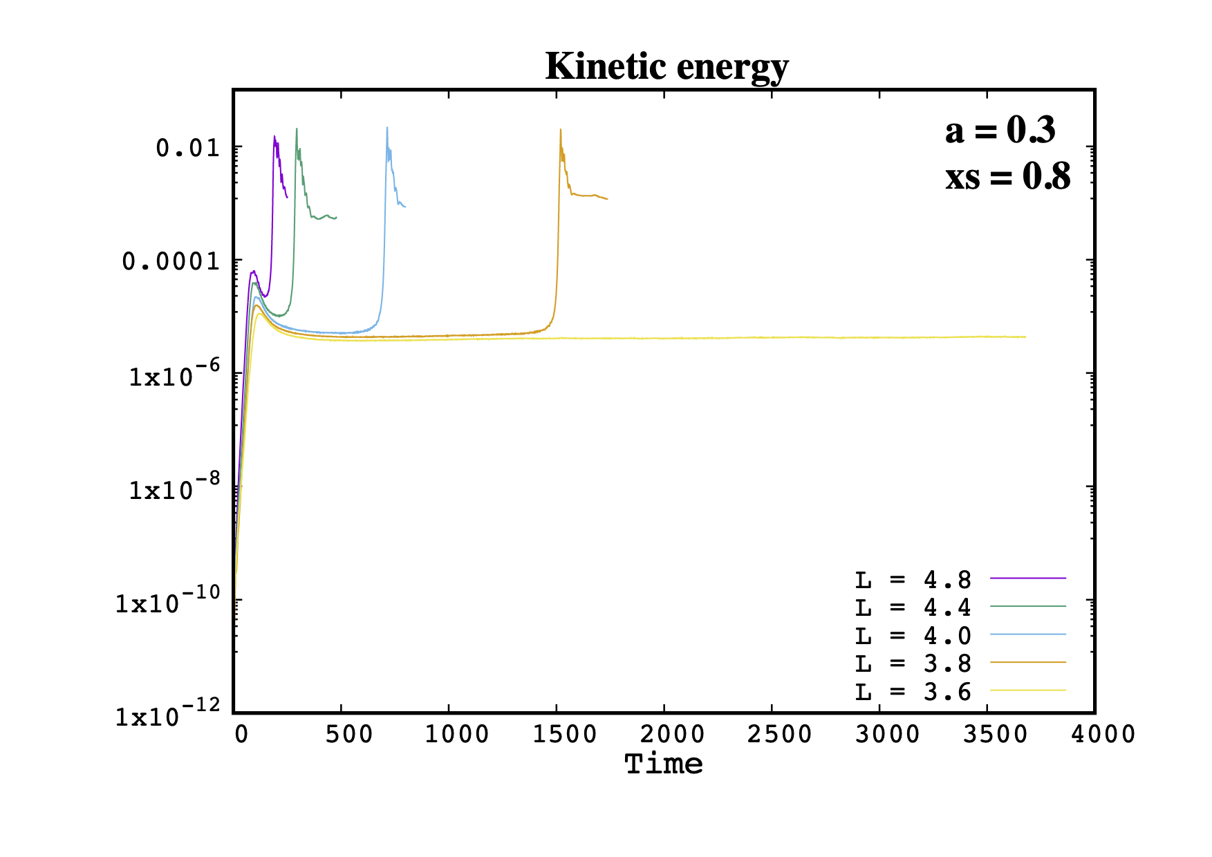
Figure 5: Time evolution of the kinetic energy $E_{K}$ for different cases employing five different length values $L=4.8,4.4,4.0,3.8,$ and $3.6$. The initial ’tanh’ equilibrium with $x_{s}=0.8$, and $a=0.3$, is taken. The other parameters are $\eta=10^{-3}$ and $P_{r}=1/3$.

3.2 On the critical aspect ratio for explosive reconnection

Following the procedure used in Janvier et al. (2011), we first explore different $L$ cases for a fixed $x_{s}$ value, that is $x_{s}=0.8$ as taken for the reference case just above. The results using the kinetic energy evolution as the main diagnostic to discriminate between stability and nonlinear destabilization, are plotted in Figure 5. Indeed, one can clearly see that the critical $L_{c}$ value for our configuration is estimated to be close to $3.7$, as the case using $L=3.6$ does not exhibit any abrupt nonlinear growth (contrary to the case with $L=3.8$). Indeed, the non linearly stable simulation ends up with saturated magnetic islands with structure similar to the last panel shown in Figure 3. The critical aspect ratio for $L/x_{s}$ is thus estimated to be $3.75/0.8\simeq 4.7$, that is a value comparable but slightly lower than the value of $5$ expected for ’sech’ profile (Janvier et al., 2011).

Second, we have investigated the dependence on the equilibrium shear at $x_{s}$, by varying $a$ between $0.2$ and $0.4$. The same critical value $L_{c}\simeq 3.75$ value is recovered whatever the shear value, as illustrated in Figure 6 (left panel) for $a=0.2$ case. We can thus conclude to the independence of the critical aspect ratio with the shear for our ’tanh’ equilibrium profile. The reader must note that the minimum length value for linear DTM instability is $L_{min}=1.26$ and $3.1$ for $a=0.2$ and $a=0.4$ respectively. Thus, $L_{min}$ remains lower than $L_{c}$ for both cases.

Finally, we have investigated the dependence on the distance between the two current sheets by varying the $x_{s}$ parameter. The results obtained for a run using $x_{s}=0.5$ and $a=0.2$ are plotted in right panel of Figure 6. Now, a smaller critical value $L_{c}\simeq 2.35$ (as it is in the range between $2.3$ and $2.4$) can be deduced for this case, leading again to the same critical aspect ratio value of $L_{c}/x_{s}=4.7$.

We conclude that the critical aspect ratio for the destabilization of the non linear instability is clearly independent of the details of the equilibrium for the double Harris-like ’tanh’ profile. Moreover, it is probably only slightly dependent of the whole profile itself when comparing the value of order $5$ previously obtained for the ’sech’ configuration by Janvier et al. (2011). This could be due to the presence of the extra magnetic gradient in the outer region (i.e. for $x\geq x_{s}$ or $x\leq-x_{s}$) embedding the two current sheets for the ’sech’ profile (see Figure 1). Indeed, It has been shown that the presence of external current can influence the growth and also saturation level of the magnetic island for the single tearing mode evolution (Poyé et al., 2013). However, we would draw the attention of the reader to the fact that the difference could also be attributed to the different numerical treatment in the two studies.

By exploring additional cases employing another resistivity value (with $\eta=3\times 10^{-4}$), we have checked that the critical aspect ratio is not resistivity-dependent in agreement with the conclusion previously drawn (Janvier et al., 2011).

3.3 On the time scale of the explosive reconnection

Another important question concerns the characteristic time scale for the explosive growth phase. It has been previously shown that it is very weakly dependent or even independent of the resistivity (Wang et al., 2007; Janvier et al., 2011; Zhang & Ma, 2011; Akramov & Baty, 2017). Moreover, the growth is shown to be faster than a simple exponential growth, i.e. faster than a scaling law $\sim\exp(\gamma^{*}t)$ for the perturbed quantities like the kinetic energy, where $\gamma^{*}$ represents an instantaneous growth rate. Janvier et al. (2011) suggest a time dependence of the form $\sim\exp\ [t\ e^{(\gamma^{*}t)}]$, and on another hand Akramov & Baty (2017) propose another form $\sim\exp(\gamma^{*}t^{2})$.

In this work, we have examined the time dependence using the kinetic energy variation during the explosive growth, and we have found that it follows another super-exponential growth. Indeed, we obtained that, our results can be the best fitted by a double exponential dependence of the form, $E_{k}\sim\exp[e^{(\gamma^{*}(t-t_{0})})]$, where $t_{0}$ represents a time instant that can be considered to be close to the onset of the explosive growth phase. This is illustrated in Figure 6, for the representative case presented above in this paper. More precisely, we used $t_{0}=688\ t_{A}$ and $\gamma^{*}=0.1\ t_{A}^{-1}$, in order to correctly approximate the explosive phase in the range of time values $[688:710]$. For earlier times the non linear instability is not yet triggered, and for later times a saturation ensues due to the final relaxation (see Figure 2). Remarkably, this result holds with the same pseudo-rate value of $\gamma^{*}\simeq 0.1\ t_{A}^{-1}$ independently of the details of the ’tanh’ equilibrium. Finally, we have also checked that the result is true for different unstable $L>L_{c}$ values, meaning that it is also independent of the ’distance’ from the non linear threshold $L-L_{c}$. This latter point was already visible when comparing the different explosive phases plotted in Figures 5-6. We complement that, it is obviously different when $L-L_{c}$ is too high as the Rutherford regime is absent.

One must note that such double exponential growth has been shown to be possible in pure 2D incompressible hydrodynamics due to unstable configurations driven by the vorticity gradient (Denisov, 2015; Kiselev & Sverak, 2014).

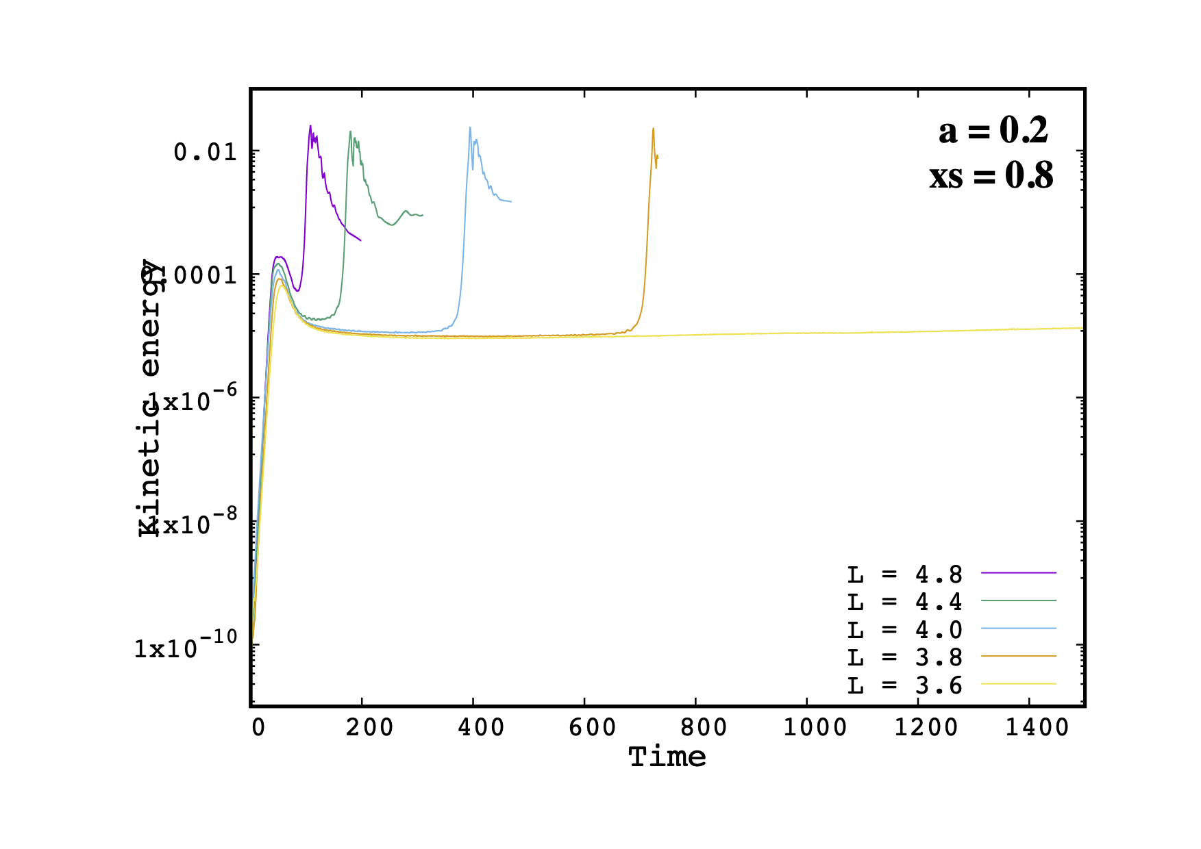
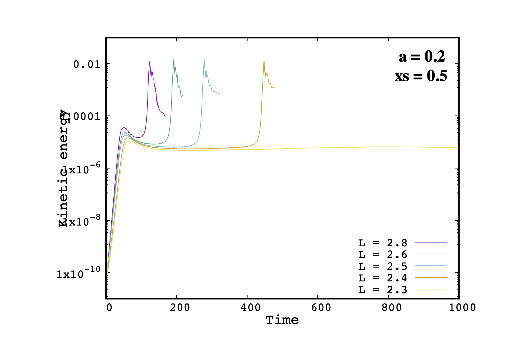
Figure 6: Time evolution of the kinetic energy $E_{K}$ for cases employing five different length value (see legend). A ’tanh’ equilibrium is employed with $x_{s}=0.8$ and $a=0.2$, and with $x_{s}=0.5$ and $a=0.2$, in left and right panel respectively.

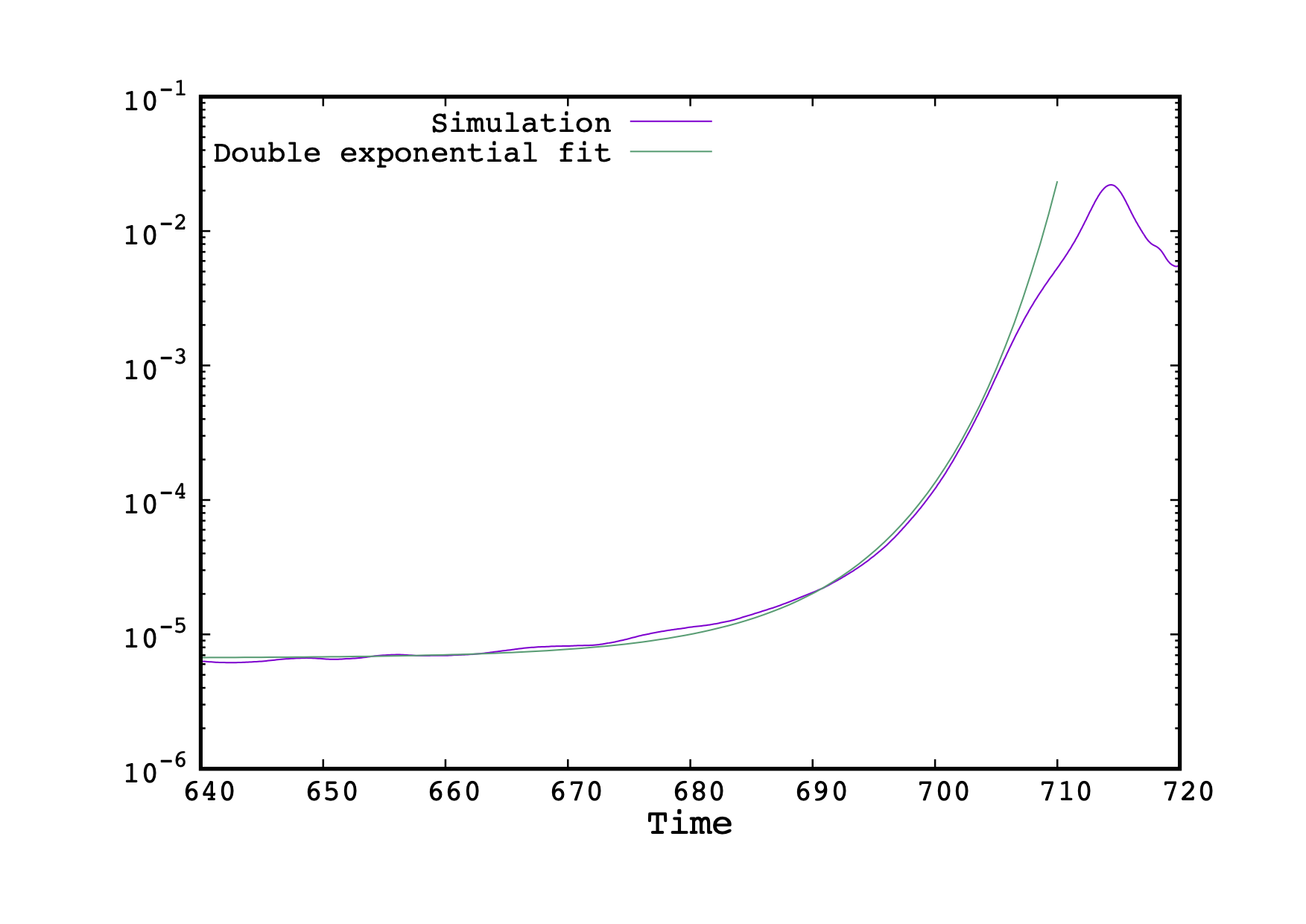
Figure 7: Zoom (centered on the explosive phase) of the time evolution of the kinetic energy for the representative ’tanh’ equilibrium case using $a=0.3$ and $x_{s}=0.8$. A double exponential fit curve following a law $\sim\exp[\exp(\gamma^{*}(t-t_{0}))]$ with $t_{0}=688$ and $\gamma^{*}=0.1$ is also plotted for comparison.

4 Conclusion

In this work, we have confirmed the existence of a critical aspect ratio $L_{c}/x_{s}$ for the non linear explosive growth in double current sheet systems. Its value is independent of the details of the magnetic equilibrium, and is obtained to be $L/x_{s}\simeq 4.7$ for the double Harris-like ’tanh’ profile considered in this study. This threshold value is similar and slightly smaller that the one (value close to $5$) deduced by Janvier et al. (2011) on the basis of another MHD equilibrium, namely the ’sech’ profile. The latter small departure could be attributed to the difference in equilibrium current density in the outer region, or to the different numerical procedure. More work is thus needed in order to further explore this point.

Second, we have examined the time dependence of the explosive phase. As shown in previous studies, we confirm the super-exponential increase of the kinetic energy $E_{K}$, as it is faster than a simple exponential law. Moreover, our results suggest that the latter follows a double exponential law of the form $E_{k}\sim\exp[\exp(\gamma^{*}(t-t_{0}))]$. The value of the characteristic parameter called pseudo-growth rate is $\gamma^{*}\simeq 0.1\ t_{A}^{-1}$, leading to a characteristic time of the order of the Alfvén time.

Our results are relevant in the context of plasma environments where multiple current layers can form. This is the case for many astrophysical plasma systems, such as the solar photosphere, solar corona, solar wind, and pulsar wind nebula. In such environment, it is well known that disruptive events leading to magnetic energy release in a sudden way are observed. Fast time scale comparable or even smaller than the Alfvén one is also required to explain the whole duration of the event. Thus, the explosive non linear DTM mechanism is a possible route for such disruptions. A second route is provided by the development of plasmoid chains in the current sheets, when the current layers are able to reach very large aspect ratio (i.e. for very long and/or very thin sheets) at least $\simeq S_{L}^{1/3}$, where $S_{L}=LV_{A}/\eta$ (Huang et al., 2017; Baty, 2020a, b, c). This would give aspect ratios higher than $10^{3}-10^{4}$ much higher than the values for $L/a$ of the order $10-20$ considered in this work. In this latter case, an explosive and reconnection mechanism can also be triggered on a time scale that can ever be smaller than the Alfvén one (Pucci & Velli, 2014; Comisso et al., 2017). Finally, the two routes are non exclusive, as the two mechanisms can also be at work in a simultaneous way (Baty, 2017). Anyway, a more realistic study would require to include the initial process of formation of the two current sheets, that are assumed to be preformed in the present work.

References

- Akramov & Baty (2017) Akramov, T., & Baty, H. 2017, PoP, 24, 082116, https://doi.org/10.1063/1.5000273
- Baty (2017) Baty, H. 2017, ApJ, 837, 74, https://doi.org/10.3847/1538-4357/aa60bd
- Baty (2019) Baty, H. 2019, ApJSS, 243, 23, https://doi.org/10.3847/1538-4365/ab2cd2
- Baty (2020a) Baty, H. 2020a, arXiv:2001.07036 https://ui.adsabs.harvard.edu/abs/2020arXiv200107036B
- Baty (2020b) Baty, H. 2020b, arXiv:2003.08660 https://ui.adsabs.harvard.edu/abs/2020arXiv200308660B
- Baty (2020c) Baty, H. 2020c, arXiv:2006.15013 https://ui.adsabs.harvard.edu/abs/2020arXiv200615013B
- Biskamp (2009) Biskamp, D. 2009, Nonlinear Magnetohydrodynamics, (Cambridge University Press). https://doi.org/10.1017/CBO9780511599965
- Comisso et al. (2017) Comisso, L., Lingam, L., Huang, Y. M., & Bhattacharjee, A. 2017, ApJ, 850, 142, https://doi.org/10.3847/1538-4357/aa9789
- Denisov (2015) Denisov, S. A. 2015, Proc. Amer. Math. Soc. 143, 1199-1210, https://arxiv.org/pdf/1201.1771.pdf
- Huang et al. (2017) Huang, Y. M., Comisso, L., & Bhattacharjee, A. 2017, ApJ, 849, 75, https://doi.org/10.3847/1538-4357/aa906d
- Ishii et al. (2002) Ishii, Y., Azumi, M., & Kishimoto, Y. 2002, PRL, 89, 205002, https://doi.org/10.1103/PhysRevLett.89.205002
- Kiselev & Sverak (2014) Kiselev, A., & Sverak, V. 2014, Annals of Mathematics Vol. 180, No. 3, 1205-1220, https://arxiv.org/pdf/1310.4799.pdf
- Janvier et al. (2011) Janvier, M., Kishimoto, M. Y., & Li, J. Q. 2011, PRL, 107, 195001, https://doi.org/10.1103/PhysRevLett.107.195001
- Priest & Forbes (2000) Priest, E. R., & Forbes, T. G. 2000, Magnetic Reconnection (Cambridge: Cambridge Univ. Press), https://doi.org/10.1017/CBO9780511525087
- Poyé et al. (2013) Poyé., A., Agullo, O., Smolyakov, A., Benkadda, S., & Garbet, X. 2013, PoP, 20, 020702, https://doi.org/10.1063/1.4791653
- Pucci & Velli (2014) Pucci, F., & Velli, M. 2014, ApJL, 780, L19, https://doi.org/10.1088/2041-8205/780/2/L19
- Wang et al. (2007) Wang, Z. X., Dong, J. Q., Lei, Y. A., Long, Y. X., Mou, Z. Z., & Qu, W. X. 2007, PRL, 99, 185004, https://doi.org/10.1103/PhysRevLett.99.185004
- Wei et al. (2020) Wei, L., Yu, F., Ren, H. J., & Wang, Z. X. 2010, AIP Advances, 10, 055111, https://doi.org/10.1063/5.0007522
- Zhang & Ma (2011) Zhang, C. L., & Ma, Z. W. 2011, PoP, 18, 052303, https://doi.org/10.1063/1.3581064