KalmanNet: Neural Network Aided Kalman Filtering for Partially Known Dynamics

Abstract

State estimation of dynamical systems in rt is a fundamental task in signal processing. For systems that are well-represented by a fully known lg ss (ss) model, the celebrated kf (kf) is a low complexity optimal solution. However, both linearity of the underlying ss model and accurate knowledge of it are often not encountered in practice. Here, we present kn, a rt state estimator that learns from data to carry out Kalman filtering under non-linear dynamics with partial information. By incorporating the structural ss model with a dedicated rnn module in the flow of the kf, we retain data efficiency and interpretability of the classic algorithm while implicitly learning complex dynamics from data. We demonstrate numerically that kn overcomes non-linearities and model mismatch, outperforming classic filtering methods operating with both mismatched and accurate domain knowledge.

I Introduction

Estimating the hidden state of a dynamical system from noisy observations in rt is one of the most fundamental tasks in signal processing and control, with applications in localization, tracking, and navigation [2]. In a pioneering work from the early 1960s [3, 4, 5], based on work by Wiener from 1949 [6], Rudolf Kalman introduced the kf, a mmse (mmse) estimator that is applicable to time-varying systems in dt, which are characterized by a linear ss model with awgn (awgn). The low-complexity implementation of the kf, combined with its sound theoretical basis, resulted in it quickly becoming the leading workhorse of se in systems that are well described by ss models in dt. The kf has been applied to problems such as radar target tracking [7], trajectory estimation of ballistic missiles [8], and estimating the position and velocity of a space vehicle in the Apollo program [9].

While the original kf assumes linear ss models, many problems encountered in practice are governed by nl dynamical equations. Therefore, shortly after the introduction of the original kf, nl variations of it were proposed, such as the ekf (ekf) [7, 8] and the ukf (ukf) [10]. Methods based on sequential mc (mc) sampling, such as the family of pf [11, 12, 13], were introduced for state estimation in nl, non-Gaussian ss models. To date, the kf and its nl variants are still widely used for online filtering in numerous rw applications involving tracking and localization [14].

The common thread among these aforementioned filters is that they are mb (mb) algorithms; namely, they rely on accurate knowledge and modeling of the underlying dynamics as a fully characterized ss model. As such, the performance of these mb methods critically depends on the validity of the domain knowledge and model assumptions. mb filtering algorithms designed to cope with some level of uncertainty in the ss models, e.g., [15, 16, 17], are rarely capable of achieving the performance of mb filtering with full domain knowledge, and rely on some knowledge of how much their postulated model deviates from the true one. In many practical use cases the underlying dynamics of the system is nl, complex, and difficult to accurately characterize as a tractable ss model, in which case degradation in performance of the mb state estimators is expected.

Recent years have witnessed remarkable empirical success of dnn in real-life applications. These dd (dd) parametric models were shown to be able to catch the subtleties of complex processes and replace the need to explicitly characterize the domain of interest [18, 19]. Therefore, an alternative strategy to implement se—without requiring explicit and accurate knowledge of the ss model—is to learn this task from data using deep learning. dnn such as rnn—i.e., lstm (lstm) [20] and gru [21]—and attention mechanisms [22] have been shown to perform very well for time series related tasks mostly in intractable environments, by training these networks in an e2e, model-agnostic manner from a large quantity of data. Nonetheless, dnn do not incorporate domain knowledge such as structured ss models in a principled manner. Consequently, these dd approaches require many trainable parameters and large data sets even for simple sequences [23] and lack the interpretability of mb methods. These constraints limit the use of highly parametrized dnn for rt se in applications embedded in hardware-limited mobile devices such as drones and vehicular systems.

The limitations of mb Kalman filtering and dd se motivate a hybrid approach that exploits the best of both worlds; i.e., the soundness and low complexity of the classic kf, and the model-agnostic nature of dnn. Therefore, we build upon the success of our previous work in mb dl for signal processing and digital communication applications [24, 25, 26, 27] to propose a hybrid mb/dd online recursive filter, coined kn. In particular, we focus on rt se for continuous-value ss models for which the kf and its variants are designed. We assume that the noise statistics are unknown and the underlying ss model is partially known or approximated from a physical model of the system dynamics. To design kn, we identify the kg (kg) computation of the kf as a critical component encapsulating the dependency on noise statistics and domain knowledge, and replace it with a compact rnn of limited complexity that is integrated into the kf flow. The resulting system uses labeled data to learn to carry out Kalman filtering in a supervised manner.

Our main contributions are summarized as follows:

1. We design kn, which is an interpretable, low complexity, and data-efficient dnn-aided rt state estimator. kn builds upon the flow and theoretical principles of the kf, incorporating partial domain knowledge of the underlying ss model in its operation.

2. By learning the kg, kn circumvents the dependency of the kf on knowledge of the underlying noise statistics, thus bypassing numerically problematic matrix inversions involved in the kf equations and overcoming the need for tailored solutions for nl systems; e.g., approximations to handle non-linearities as in the ekf.

3. We show that kn learns to carry out kfing from data in a manner that is invariant to the sequence length. Specifically, we present an efficient supervised training scheme that enables kn to operate with arbitrary long trajectories while only training using short trajectories.

4. We evaluate kn in various ss models. The experimental scenarios include synthetic setups, tracking the chaotic Lorenz system, and localization using the Michigan nclt ds [28]. kn is shown to converge much faster compared with purely dd systems, while outperforming the mb ekf, ukf, and pf, when facing model mismatch and dominant non-linearities.

The proposed kn leverages data and partial domain knowledge to learn the filtering operation, rather than using data to explicitly estimate the missing ss model parameters. Although there is a large body of work that combines ss models with dnn, e.g., [29, 30, 31, 32, 33, 34, 35], these approaches are sometimes used for different ss related tasks (e.g., smoothing, imputation); with a different focus, e.g., incorporating high-dimensional visual observations to a kf; or under different assumptions, as we discuss in detail below.

The rest of this paper is organized as follows: Section II reviews the ss model and its associated tasks, and discusses related works. Section III details the proposed kn. Section IV presents the numerical study. Section V provides concluding remarks and future work.

Throughout the paper, we use boldface lower-case letters for vectors and boldface upper-case letters for matrices. The transpose, $\ell_{2}$ norm, and stochastic expectation are denoted by $\left\{\cdot\right\}^{\top}$, $\left\|\cdot\right\|$, and $\mathds{E}\left[\cdot\right]$, respectively. The Gaussian distribution with mean $\mathbf{\mu}$ and covariance $\mathbf{\Sigma}$ is denoted by $\mathcal{N}(\mathbf{\mu},\mathbf{\Sigma})$. Finally, $\mathbb{R}$ and $\mathbb{Z}$ are the sets of real and integer numbers, respectively.

II System Model and Preliminaries

II-A State Space Model

We consider dynamical systems characterized by a ss model in dt [36]. We focus on (possibly) nl, Gaussian, and continuous ss models, which for each $t\in\mathbb{Z}$ are represented via

$$\mathbf{x}_{t} =\mathbf{f}\left(\mathbf{x}_{t-1}\right)+\mathbf{w}_{t}, \mathbf{w}_{t}\sim\mathcal{N}\left(\mathbf{0},\mathbf{Q}\right),\hskip 7.11317pt \mathbf{x}_{t}\in\mathbb{R}^{m},$$ (1a)

$$\mathbf{y}_{t} =\mathbf{h}\left(\mathbf{x}_{t}\right)+\mathbf{v}_{t}, \mathbf{v}_{t}\sim\mathcal{N}\left(\mathbf{0},\mathbf{R}\right),\hskip 7.11317pt \mathbf{y}_{t}\in\mathbb{R}^{n}.$$ (1b)

In (1a), $\mathbf{x}_{t}$ is the latent state vector of the system at time $t$, which evolves from the previous state $\mathbf{x}_{t-1}$, by a (possibly) nl, state-evolution function $\mathbf{f}\left(\cdot\right)$ and by an awgn $\mathbf{w}_{t}$ with covariance matrix $\mathbf{Q}$. In (1b), $\mathbf{y}_{t}$ is the vector of observations at time $t$, which is generated from the current latent state vector by a (possibly) nl observation (emission) mapping $\mathbf{h}\left(\cdot\right)$ corrupted byawgn $\mathbf{v}_{t}$ with covariance $\mathbf{R}$. For the special case where the evolution or the observation transformations are linear, there exist matrices $\mathbf{F},\mathbf{H}$ such that

$$\mathbf{f}\left(\mathbf{x}_{t-1}\right)={\mathbf{F}}\cdot\mathbf{x}_{t-1},\quad\mathbf{h}\left(\mathbf{x}_{t}\right)={\mathbf{H}}\cdot\mathbf{x}_{t}.$$ (2)

In practice, the state-evolution model (1a) is determined by the complex dynamics of the underlying system, while the observation model (1b) is dictated by the type and quality of the observations. For instance, $\mathbf{x}_{t}$ can determine the location, velocity, and acceleration of a vehicle, while $\mathbf{y}_{t}$ are measurements obtained from several sensors. The parameters of these models may be unknown and often require the introduction of dedicated mechanisms for their estimation in real-time [37, 38]. In some scenarios, one is likely to have access to an approximated or mismatched characterization of the underlying dynamics.

ss models are studied in the context of several different tasks; these tasks are different in their nature, and can be roughly classified into two main categories: observation approximation and hidden state recovery. The first category deals with approximating parts of the observed signal $\mathbf{y}_{t}$. This can correspond, for example, to the prediction of future observations given past observations; the generation of missing observations in a given block via imputation; and the denoising of the observations. The second category considers the recovery of a hidden state vector $\mathbf{x}_{t}$. This family of state recovery tasks includes offline recovery, also referred to as smoothing, where one must recover a block of hidden state vectors, given a block of observations, e.g., [35]. The focus of this paper is filtering; i.e., online recovery of $\mathbf{x}_{t}$ from past and current noisy observations $\{\mathbf{y}_{\tau}\}_{\tau=1}^{t}$. For a given $\mathbf{x}_{0}$, filtering involves the design of a mapping from $\mathbf{y}_{t}$ to $\hat{\mathbf{x}}_{t}$, $\forall t\in\left\{1,2,\ldots,T\right\}\triangleq\mathcal{T}$, where $T$ is the time horizon.

II-B Data-Aided Filtering Problem Formulation

The filtering problem is at the core of rt tracking. Here, one must provide an instantaneous estimate of the state ${\mathbf{x}}_{t}$ based on each incoming observation $\mathbf{y}_{t}$ in an online manner. Our main focus is on scenarios where one has partial knowledge of the ss model that describes the underlying dynamics. Namely, we know (or have an approximation of) the state-evolution (transition) function $\mathbf{f}\left(\cdot\right)$ and the state-observation (emission) function $\mathbf{h}\left(\cdot\right)$. For rw applications, this knowledge is derived from our understating of the system dynamics, its physical design, and the model of the sensors. As opposed to the classical assumptions in kf, the noise statistics $\mathbf{Q}$ and $\mathbf{R}$ are not known. More specifically, we assume:

• Knowledge of the distribution of the noise signals $\mathbf{w}_{t}$ and $\mathbf{v}_{t}$ is not available.

• The functions $\mathbf{f}\left(\cdot\right)$ and $\mathbf{h}\left(\cdot\right)$ may constitute an approximation of the true underlying dynamics. Such approximations can correspond, for instance, to the representation of continuous time dynamics in discrete time, acquisition using misaligned sensors, and other forms of mismatches.

While we focus on filtering in partially known ss models, we assume that we have access to a labeled ds containing a sequence of observations and their corresponding gt states. In various scenarios of interest, one can assume access to some gt measurements in the design stage. For example, in field experiments it is possible to add extra sensors both internally or externally to collect the gt needed for training. It is also possible to compute the gt data using offline and more computationally intensive algorithms. Finally, the inference complexity of the learned filter should be of the same order (and preferably smaller) as that of mb filters, such as the ekf.

II-C Related Work

A key ingredient in recursive Bayesian filtering is the update operation; namely, the need to update the prior estimate using new observed information. For lg ss using the kf, this boils down to computing the kg. While the kf assumes linear ss models, many problems encountered in practice are governed by nl dynamics, for which one should resort to approximations. Several extensions of the kf were proposed to deal with non-linearities. The ekf [7, 8] is a quasi-linear algorithm based on an analytical linearization of the ss model. More recent nl variations are based on numerical integration: ukf [10], the Gauss-Hermite Quadrature [39], and the Cubature kf [40]. For more complex ss models, and when the noise cannot be modeled as Gaussian, multiple variants of the pf were proposed that are based on sequential mc [11, 12, 13, 41, 42, 43, 44, 45]. These mc algorithms are considered to be asymptotically exact but relatively computationally heavy when compared to Kalman-based algorithms. These mb algorithms require accurate knowledge of the ss model, and their performance is typically degrades in the presence of model mismatch.

The combination of ml and ss models, and specifically Kalman-based algorithms, is the focus of growing research attention. To frame the current work in the context of existing literature, we focus on the approaches that preserve the general structure of the ss model. The conventional approach to deal with partially known ss models is to impose a parametric model and then estimate its parameters. This can be achieved by jointly learning the parameters and state sequence using em [46, 47, 48] and Bayesian probabilistic algorithms [37, 38], or by selecting from a set of a priori known models [49]. When training data is available, it is commonly used to tune the missing parameters in advance, in a supervised or an unsupervised manner, as done in [50, 51, 52]. The main drawback of these strategies is that they are restricted to an imposed parametric model on the underlying dynamics (e.g., Gaussian noises).

When one can bound the uncertainty in the ss model in advance, an alternative approach to learning is to minimize the worst-case estimation error among all expected ss models. Such robust variations were proposed for various state estimation algorithms, including Kalman variants [53, 15, 16, 17] and particle filters [54, 55]. The fact that these approaches aim to design the filter to be suitable for multiple different ss models typically results in degraded performance compared to operating with known dynamics.

When the underlying system’s dynamics are complex and only partially known or the emission model is intractable and cannot be captured in a closed form—e.g., visual observations as in a computer vision task [56]—one can resort to approximations and to the use of dnn. Variational inference [57, 58, 59] is commonly used in connection with ss models, as in [29, 33, 30, 34, 31], by casting the Bayesian inference task to optimization of a parameterized posterior and maximizing an objective. Such approaches cannot typically be applied directly to state recovery in rt, as we consider here, and the learning procedure tends to be complex and prone to approximation errors.

A common strategy when using dnn is to encode the observations into some latent space that is assumed to obey a simple ss model, typically a linear Gaussian one, and track the state in the latent domain as in [60, 61, 56], or to use dnn to estimate the parameters of the ss model as in [62, 63]. Tracking in the latent space can also be extended by applying a dnn decoder to the estimated state to return to the observations domain, while training the overall system end-to-end [31, 64]. The latter allows to design trainable systems for recovering missing observations and predicting future ones by assuming that the temporal relationship can be captured as an ss model in the latent space. This form of dnn-aided systems is typically designed for unknown or highly complex ss models, while we focus in this work on setups with partial domain knowledge, as detailed in Subsection II-B. Another approach is to combine rnn [65], or variational inference [66, 32] with mc based sampling. Also related is the work [35], which used learned models in parallel with mb algorithms operating with full knowledge of the ss model, applying a graph neural network in parallel to the Kalman smoother to improve its accuracy via neural augmentation. Estimation was performed by an iterative message passing over the entire time horizon. This approach is suitable for the smoothing task and is computationally intensive, and so may not be suitable for rt filtering [67].

II-D Model-Based Kalman Filtering

Our proposed kn, detailed in the following section, is based on the mb kf, which is a linear recursive estimator. In every time step $t$, the kf produces a new estimate $\mathbf{x}_{t}$ using only the previous estimate $\hat{\mathbf{x}}_{t-1}$ as a sufficient statistic and the new observation $\mathbf{y}_{t}$. As a result, the computational complexity of the kf does not grow in time. We first describe the original algorithm for linear ss models, as in (2), and then discuss how it is extended into the ekf for nl ss models.

The kf can be described by a two-step procedure: prediction and update, where in each time step $t\in\mathcal{T}$, it computes the first- and second-order statistical moments.

1. The first step predicts the current a priori statistical moments based on the previous a posteriori estimates. Specifically, the moments of $\mathbf{x}$ are computed using the knowledge of the evolution matrix $\mathbf{F}$ as

   $$\hat{\mathbf{x}}_{t\left|t-1\right.} =\mathbf{F}\cdot{\hat{\mathbf{x}}_{t-1\left|t-1\right.}},$$ (3a)

   $$\boldsymbol{\Sigma}_{t\left|t-1\right.} ={\mathbf{F}}\cdot\boldsymbol{\Sigma}_{t-1\left|t-1\right.}\cdot{\mathbf{F}}^{\top}+\mathbf{Q}$$ (3b)

   and the moments of the observations $\mathbf{y}$ are computed based on the knowledge of the observation matrix $\mathbf{H}$ as

   $$\hat{\mathbf{y}}_{t\left|t-1\right.} =\mathbf{H}\cdot\hat{\mathbf{x}}_{t\left|t-1\right.}$$ (4a)

   $${\mathbf{S}}_{t\left|t-1\right.} ={\mathbf{H}}\cdot\boldsymbol{\Sigma}_{t\left|t-1\right.}\cdot{\mathbf{H}}^{\top}+\mathbf{R}.$$ (4b)

2. In the update step, the a posteriori state moments are computed based on the a priori moments as

   $$\hat{\mathbf{x}}_{t\left|t\right.} =\hat{\mathbf{x}}_{t\left|t-1\right.}+\mathbfcal{K}_{t}\cdot\Delta\mathbf{y}_{t}$$ (5a)

   $${\boldsymbol{\Sigma}}_{t\left|t\right.} ={\boldsymbol{\Sigma}}_{t\left|t-1\right.}-\mathbfcal{K}_{t}\cdot{\mathbf{S}}_{t\left|t-1\right.}\cdot\mathbfcal{K}^{\top}_{t}.$$ (5b)

   Here, $\mathbfcal{K}_{t}$ is the kg, and it is given by

   $$\mathbfcal{K}_{t}={\boldsymbol{\Sigma}}_{t\left|t-1\right.}\cdot{\mathbf{H}}^{\top}\cdot{\mathbf{S}}^{-1}_{t\left|t-1\right.}.$$ (6)

   The term $\Delta\mathbf{y}_{t}$ is the innovation; i.e., the difference between the predicted observation and the observed value, and it is the only term that depends on the observed data

   $$\Delta\mathbf{y}_{t}=\mathbf{y}_{t}-\hat{\mathbf{y}}_{t\left|t-1\right.}.$$ (7)

The ekf extends the kf for nl $\mathbf{f}\left(\cdot\right)$ and/or $\mathbf{h}\left(\cdot\right)$, as in (1). Here, the first-order statistical moments (3a) and (4a) are replaced with

$$\hat{\mathbf{x}}_{t\left|t-1\right.} =\mathbf{f}\left(\hat{\mathbf{x}}_{t-1}\right),$$ (8a)

$$\hat{\mathbf{y}}_{t\left|t-1\right.} =\mathbf{h}\left(\hat{\mathbf{x}}_{t\left|t-1\right.}\right),$$ (8b)

respectively. The second-order moments, though, cannot be propagated through the non-linearity, and must thus be approximated. The ekf linearizes the differentiable $\mathbf{f}\left(\cdot\right)$ and $\mathbf{h}\left(\cdot\right)$ in a time-dependent manner using their partial derivative matrices, also known as Jacobians, evaluated at $\hat{\mathbf{x}}_{t-1\left|t-1\right.}$ and $\hat{\mathbf{x}}_{t\left|t-1\right.}$. Namely,

$$\hat{\mathbf{F}}_{t} =\mathcal{J}_{\mathbf{f}}\left(\hat{\mathbf{x}}_{t-1\left|t-1\right.}\right)$$ (9a)

$$\hat{\mathbf{H}}_{t} =\mathcal{J}_{\mathbf{h}}\left(\hat{\mathbf{x}}_{t\left|t-1\right.}\right),$$ (9b)

where $\hat{\mathbf{F}}_{t}$ is plugged into (3b) and $\hat{\mathbf{H}}_{t}$ is used in (4b) and (6). When the ss model is linear, the ekf coincides with the kf, which achieves the mmse for linear Gaussian ss models.

An illustration of the ekf is depicted in Fig. 1. The resulting filter admits an efficient linear recursive structure. However, it requires full knowledge of the underlying model and notably degrades in the presence of model mismatch. When the model is highly nl, the local linearity approximation may not hold, and the ekf can result in degraded performance. This motivates the augmentation of the ekf into the deep learning-aided kn, detailed next.

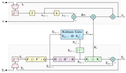
Figure 1: ekf block diagram. Here, $\mathcal{Z}^{-1}$ is the unit delay.

III KalmanNet

Here, we present kn; a hybrid, interpretable, data efficient architecture for rt se in nl dynamical systems with partial domain knowledge. kn combines mb Kalman filtering with an rnn to cope with model mismatch and non-linearities. To introduce kn, we begin by explaining its high level operation in Subsection III-A. Then we present the features processed by its internal rnn and the specific architectures considered for implementing and training kn in Subsections III-B-III-D. Finally, we provide a discussion in Subsection III-E.

III-A High Level Architecture

We formulate kn by identifying the specific computations of the ekf that are based on unavailable knowledge. As detailed in Subsection II-B, the functions $\mathbf{f}\left(\cdot\right)$ and $\mathbf{h}\left(\cdot\right)$ are known (though perhaps inaccurately); yet the covariance matrices $\mathbf{Q}$ and $\mathbf{R}$ are unavailable. These missing statistical moments are used in mb Kalman filtering only for computing the kg (see Fig. 1). Thus, we design kn to learn the kg from data, and combine the learned kg in the overall kf flow. This high level architecture is illustrated in Fig. 2.

In each time instance $t\in\mathcal{T}$, similarly to the ekf, kn estimates $\hat{\mathbf{x}}_{t}$ in two steps; prediction and update.

1. The prediction step is the same as in the mb ekf, except that only the first-order statistical moments are predicted. In particular, a prior estimate for the current state $\hat{\mathbf{x}}_{t\left|t-1\right.}$ is computed from the previous posterior $\hat{\mathbf{x}}_{t-1}$ via (8a). Then, a prior estimate for the current observation $\hat{\mathbf{y}}_{t\left|t-1\right.}$ is computed from $\hat{\mathbf{x}}_{t\left|t-1\right.}$ via (8b). As opposed to its mb counterparts, kn does not rely on the knowledge of noise distribution and does not maintain an explicit estimate of the cov.

2. In the update step, kn uses the new observation $\mathbf{y}_{t}$ to compute the current state posterior $\hat{\mathbf{x}}_{t}$ from the previously computed prior $\hat{\mathbf{x}}_{t\left|t-1\right.}$ in a similar manner to the mb kf as in (5a), i.e., using the innovation term $\Delta\mathbf{y}_{t}$ computed via (7) and the kg $\mathbfcal{K}_{t}$. As opposed to the mb ekf, here the computation of the kg is not given explicitly; rather, it is learned from data using an rnn, as illustrated in Fig. 2. The inherent memory of rnn allows to implicitly track the second-order statistical moments without requiring knowledge of the underlying noise statistics.

Designing an rnn to learn how to compute the kg as part of an overall kf flow requires answers to three key questions:

1. From which input features (signals) will the network learn the kg?

2. What should be the architecture of the internal rnn?

3. How will this network be trained from data?

In the following sections we address these questions.

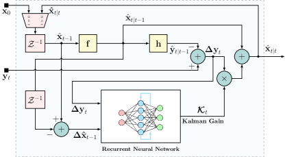
Figure 2: kn block diagram.

III-B Input Features

The mb kf and its variants compute the kg from knowledge of the underlying statistics. To implement such computations in a learned fashion, one must provide input (features) that capture the knowledge needed to evaluate the kg to a neural network. The dependence of $\mathbfcal{K}_{t}$ on the statistics of the observations and the state process indicates that in order to track it, in every time step $t\in\mathcal{T}$, the rnn should be provided with input containing statistical information of the observations $\mathbf{y}_{t}$ and the state-estimate $\hat{\mathbf{x}}_{t-1}$. Therefore, the following quantities that are related to the unknown statistical relationship of the ss model can be used as input features to the rnn:

1. The observation difference $\Delta\tilde{\mathbf{y}}_{t}={\mathbf{y}_{t}-\mathbf{y}_{t-1}}$.

2. The innovation difference $\Delta\mathbf{y}_{t}=\mathbf{y}_{t}-\hat{\mathbf{y}}_{t\left|t-1\right.}$.

3. The forward evolution difference $\Delta\tilde{\mathbf{x}}_{t}={\hat{\mathbf{x}}_{t\left|t\right.}-\hat{\mathbf{x}}_{{t-1}\left|t-1\right.}}$. This quantity represents the difference between two consecutive posterior state estimates, where for time instance $t$, the available feature is $\Delta\tilde{\mathbf{x}}_{t-1}$.

4. The forward update difference $\Delta\hat{\mathbf{x}}_{t}={\hat{\mathbf{x}}_{t\left|t\right.}-\hat{\mathbf{x}}_{{t}\left|t-1\right.}}$, i.e., the difference between the posterior state estimate and the prior state estimate, where again for time instance $t$ we use $\Delta\hat{\mathbf{x}}_{t-1}$.

Features F1 and F3 encapsulate information about the state-evolution process, while features F2 and F4 encapsulate the uncertainty of our state estimate. The difference operation removes the predictable components, and thus the time series of differences is mostly affected by the noise statistics that we wish to learn. The rnn described in Fig. 2 can use all the features, although extensive empirical evaluation suggests that the specific choice of combination of features depends on the problem at hand. Our empirical observations indicate that good combinations are {F1, F2, F4} and {F1, F3, F4}.

III-C Neural Network Architecture

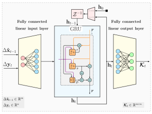
Figure 3: kn rnn block diagram (arch1). The architecture comprises a fully connected input layer, followed by a gru layer (whose internal division into gates is illustrated [21]) and an output fully connected layer. Here, the input features are F2 and F4.

The internal dnn of kn uses the features discussed in the previous section to compute the kg. It follows from (6) that computing the kg $\mathbfcal{K}_{t}$ involves tracking the cov ${\boldsymbol{\Sigma}}_{t}$. The recursive nature of the kg computation indicates that its learned module should involve an internal memory element as an rnn to track it.

We consider two architectures for the kg computing rnn. The first, illustrated in Fig. 3, aims at using the internal memory of rnn to jointly track the underlying second-order statistical moments required for computing the kg in an implicit manner. To that aim, we use gru cells [21] whose hidden state is of the size of some integer product of $m^{2}+n^{2}$, which is the joint dimensionality of the tracked moments $\hat{\mathbf{\Sigma}}_{t|t-1}$ in (3b), and $\hat{\mathbf{S}}_{t}$ in (4b). In particular, we first use a fc (fc) input layer whose output is the input to the gru. The gru state vector $\mathbf{h}_{t}$ is mapped into the estimated kg $\mathbfcal{K}_{t}\in\mathbb{R}^{m\times n}$ using an output fc layer with $m\cdot n$ neurons. While the illustration in Fig. 3 uses a single gru layer, one can also utilize multiple layers to increase the capacity and abstractness of the network, as we do in the numerical study reported in Subsection IV-E. The proposed architecture does not directly design the hidden state of the gru to correspond to the unknown second-order statistical moments that are tracked by the mb kf. As such, it uses a relatively large number of state variables that are expected to provide the required tracking capacity. For example, in the numerical study in Section IV we set the dimensionality of $\mathbf{h}_{t}$ to be $10\cdot(m^{2}+n^{2})$. This often results in substantial over-parameterization, as the number of gru parameters grows quadratically with the number of state variables [68].

The second architecture uses separate gru cells for each of the tracked cov. The division of the architecture into separate gru cells and fc layers and their interconnection is illustrated in Fig. 4. As shown in the figure, the network composes three gru layers, connected in a cascade with dedicated input and output fc layers. The first gru layer tracks the unknown state noise covariance $\mathbf{Q}$, thus tracking $m^{2}$ variables. Similarly, the second and third gru track the predicted moments $\hat{\mathbf{\Sigma}}_{t|t-1}$ (3b) and $\hat{\mathbf{S}}_{t}$ (4b), thus having $m^{2}$ and $n^{2}$ hidden state variables, respectively. The gru are interconnected such that the learned $\mathbf{Q}$ is used to compute $\hat{\mathbf{\Sigma}}_{t|t-1}$, which in turn is used to obtain $\hat{\mathbf{S}}_{t}$, while both $\hat{\mathbf{\Sigma}}_{t|t-1}$ and $\hat{\mathbf{S}}_{t}$ are involved in producing $\mathbfcal{K}_{t}$ (6). This architecture, which is composed of a non-standard interconnection between gru and fc layers, is more directly tailored towards the formulation of the ss model and the operation of the mb kf compared with the simpler first architecture. As such, it provides lesser abstraction; i.e., it is expected to be more constrained in the family of mappings it can learn compared with the first architecture, while as a result also requiring less trainable parameters. For instance, in the numerical study reported in Subsection IV-D, utilizing the first architecture requires the order of $5\cdot 10^{5}$ trainable parameters, while the second architecture utilizes merely $2.5\cdot 10^{4}$ parameters.

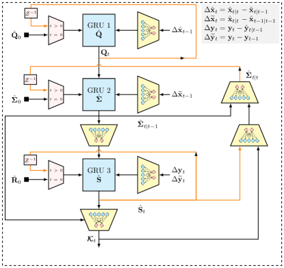
Figure 4: kn rnn block diagram (arch2). The input features are used to update three gru with dedicated fc layers, and the overall interconnection between the blocks is based on the flow of the kg computation in the mb kf.

III-D Training Algorithm

kn is trained using the available labeled data set in a supervised manner. While we use a neural network for computing the kg rather than for directly producing the estimate $\hat{\mathbf{x}}_{t|t}$, we train kn end-to-end. Namely, we compute the loss function $\mathcal{L}$ based on the state estimate $\hat{\mathbf{x}}_{t}$, which is not the output of the internal rnn. Since this vector takes values in a continuous set $\mathbb{R}^{m}$, we use the squared-error loss,

$$\mathcal{L}=\left\|\mathbf{x}_{t}-\hat{\mathbf{x}}_{t|t}\right\|^{2}$$ (10)

which is also used to evaluate the mb kf. By doing so, we build upon the ability to backpropagate the loss to the computation of the kg. One can obtain the loss gradient with respect to the kg from the output of kn since

$$\frac{\partial\mathcal{L}}{\partial\mathbfcal{K}_{t}} =\frac{\partial\left\|\mathbfcal{K}_{t}\Delta\mathbf{y}_{t}-\Delta\mathbf{x}_{t}\right\|^{2}}{\partial\mathbfcal{K}_{t}}$$

$$=2\cdot\left(\mathbfcal{K}_{t}\cdot\Delta\mathbf{y}_{t}-\Delta\mathbf{x}_{t}\right)\cdot\Delta\mathbf{y}_{t}^{\top},$$ (11)

where $\Delta\mathbf{x}_{t}\triangleq\mathbf{x}_{t}-\hat{\mathbf{x}}_{t|t-1}$. The gradient computation in (11) indicates that one can learn the computation of the kg by training kn end-to-end using the squared-error loss. In particular, this allows to train the overall filtering system without having to externally provide ground truth values of the kg for training purposes.

The data set used for training comprises $N$ trajectories that can be of varying lengths. Namely, by letting $T_{i}$ be the length of the $i$th training trajectory, the data set is given by $\mathcal{D}=\left\{(\mathbf{Y}_{i},\mathbf{X}_{i})\right\}_{1}^{N}$, where

$$\mathbf{Y}_{i} =\big{[}\mathbf{y}_{1}^{\left(i\right)},\ldots,\mathbf{y}_{T_{i}}^{\left(i\right)}\big{]},\quad\mathbf{X}_{i} =\big{[}\mathbf{x}_{0}^{\left(i\right)},\mathbf{x}_{1}^{\left(i\right)},\ldots,\mathbf{x}_{T_{i}}^{\left(i\right)}\big{]}.$$ (12)

By letting $\mathbf{\Theta}$ denote the trainable parameters of the rnn, and $\gamma$ be a regularization coefficient, we then construct an $\ell_{2}$ regularized mse (mse) loss measure

$$\ell_{i}\left(\mathbf{\Theta}\right)=\frac{1}{T_{i}}\sum_{t=1}^{T_{i}}\left\|\hat{\mathbf{x}}_{t}\left(\mathbf{y}^{\left(i\right)}_{t};\mathbf{\Theta}\right)\!-\!\mathbf{x}^{\left(i\right)}_{t}\right\|^{2}+\gamma\cdot\left\|\mathbf{\Theta}\right\|^{2}.$$ (13)

To optimize $\mathbf{\Theta}$, we use a variant of mini-batch sgd in which for every batch indexed by $k$, we choose $M<N$ trajectories indexed by $i_{1}^{k},\ldots,i_{M}^{k}$, computing the mini-batch loss as

$$\mathcal{L}_{k}\left(\mathbf{\Theta}\right)=\frac{1}{M}\sum_{j=1}^{M}\ell_{i_{j}^{k}}\left(\mathbf{\Theta}\right).$$ (14)

Since kn is a recursive architecture with both an external recurrence and an internal rnn, we use the bptt (bptt) algorithm [69] to train it. Specifically, we unfold kn across time with shared network parameters, and then compute a forward and backward gradient estimation pass through the network. We consider three different variations of applying the bptt algorithm for training kn:

1. Direct application of bptt, where for each training iteration the gradients are computed over the entire trajectory.

2. An application of the truncated bptt algorithm [70]. Here, given a ds of long trajectories (e.g., $T=3000$ time steps), each long trajectory is divided into multiple short trajectories (e.g., $T=100$ time steps), which are shuffled and used during training.

3. An alternative application of truncated bptt, where we truncate each trajectory to a fixed (and relatively short) length, and train using these short trajectories.

Overall, directly applying bptt via V1 may be computationally expensive and unstable. Therefore, a favored approach is to first use the truncated bptt as in V2 as a warm-up phase (train first on short trajectories) in order to stabilize its learning process, after which kn is tuned using V1. The procedure in V3 is most suitable for systems that are known to be likely to quickly converge to a steady state (e.g., linear ss models). In our numerical study, reported in Section IV, we utilize all three approaches.

III-E Discussion

kn is designed to operate in a hybrid dd/mb manner, combining dl with the classical ekf procedure. By identifying the specific noise-model-dependent computations of the ekf and replacing them with a dedicated rnn integrated in the ekf flow, kn benefits from the individual strengths of both dd and mb approaches. The augmentation of the ekf with dedicated deep learning modules results in several core differences between kn and its mb counterpart. Unlike the mb ekf, kn does not attempt to linearize the ss model, and does not impose a statistical model on the noise signals. In addition, kn filters in a non-linear manner, as its kg matrix depends on the input $\mathbf{y}_{t}$. Due to these differences, compared to mb Kalman filtering, kn is more robust to model mismatch and can infer more efficiently, as demonstrated in Section IV. In particular, the mb ekf is sensitive to inaccuracies in the underlying ss model, e.g., in $\mathbf{f}\left(\cdot\right)$ and $\mathbf{h}\left(\cdot\right)$, while kn can overcome such uncertainty by learning an alternative kg that yields accurate estimation.

Furthermore, kn is derived for ss models when noise statistics are not specified explicitly. A mb approach to tackle this without relying on data employs the rkf [15, 16, 17], which designs the filter to minimize the maximal mse within some range of assumed ss models, at the cost of performance loss, compared to knowing the true model. When one has access to data, the direct strategy to implement the ekf in such setups is to use the data to estimate $\mathbf{Q}$ and $\mathbf{R}$, either directly from the data or by backpropagating through the operation of the ekf as in [51], and utilize these estimates to compute the kg. As covariance estimation can be a challenging task when dealing with high-dimensional signals, kn bypasses this need by directly learning the kg, and by doing so approaches the mse of mb Kalman filtering with full knowledge of the ss model, as demonstrated in Section IV. Finally, the computation complexity for each time step $t\in\mathcal{T}$ is also linear in the rnn dimensions and does not involve matrix inversion. This implies that kn is a good candidate to apply for high dimensional ss models and on computationally limited devices.

Compared to purely dd state estimation, kn benefits from its model awareness and the fact that its operation follows the flow of mb Kalman filtering rather than being utilized as a black box. As numerically observed in Section IV, kn achieves improved mse compared to utilizing rnn for end-to-end state estimation, and also approaches the mmse performance achieved by the mb kf in linear Gaussian ss models. Furthermore, the fact that kn preserves the flow of the ekf implies that the intermediate features exchanged between its modules have a specific operation meaning, providing interpretability that is often scarce in e2e, dl systems. Finally, the fact that kn learns to compute the kg indicates the possibility of providing not only estimates of the state $\mathbf{x}_{t}$, but also a measure of confidence in this estimate, as the kg can be related to the covariance of the estimate, as initially explored in [71].

These combined gains of kn over purely mb and dd approaches were recently observed in [72], which utilized an early version of kn for rt velocity estimation in an autonomous racing car. In such a setup, a nl, mb mixed kf was traditionally used, and suffered from performance degradation due to inherent mismatches in the formulation of the ss model describing the problem. Nonetheless, previously proposed dd techniques relying on rnn for e2e state estimation were not operable in the desired frequencies on the hardware limited vehicle control unit. It was shown in [72] that the application of kn allowed to achieve improved rt velocity tracking compared to mb techniques while being deployed on the control unit of the vehicle.

Our design of kn gives rise to many interesting future extensions. Since we focus here on ss models where the mappings $\mathbf{f}\left(\cdot\right)$ and $\mathbf{h}\left(\cdot\right)$ are known up to some approximation errors, a natural extension of kn is to use the data to pre-estimate them, as demonstrated briefly in the numerical study. Another alternative to cope with these approximation errors is to utilize dedicated neural networks to learn these mappings while training the entire model in an e2e fashion. Doing so is expected to allow kn to be utilized in scenarios with analytically intractable ss models, as often arises when tracking based on unstructured observations, e.g., visual observations as in [56].

While we train kn in a supervised manner using labeled data, the fact that it preserves the operation of the mb ekf that produces a prediction of the next observation $\hat{\mathbf{y}}_{t|t-1}$ for each time instance indicates the possibility of using this intermediate feature for unsupervised training. One can thus envision kn being trained offline in a supervised manner, while tracking variations in the underlying ss model at run-time by online self supervision, following a similar rationale to that used in [24, 25] for deep symbol detection in time-varying communication channels.

Finally, we note that while we focus here on filtering tasks, ss models are used to represent additional related problems such as smoothing and prediction, as discussed in Subsection II-A. The fact that kn does not explicitly estimate the ss model implies that it cannot simply substitute these parameters into an alternative algorithm capable of carrying out tasks other than filtering. Nonetheless, one can still design dnn-aided algorithms for these tasks operating with partially known ss models as extensions of kn, in the same manner as many mb algorithms build upon the kf. For instance, as the mb kf constitutes the first part of the Rauch-Tung-Striebel smoother [73], one can extend kn to implement high-performance smoothing in partially known ss models, as we have recently began investigating in [67]. Nonetheless, we leave the exploration of extensions of kn to alternative tasks associated with ss models for future work.

IV Experiments and Results

In this section we present an extensive numerical study of kn, evaluating its performance in multiple setups and comparing it to various benchmark algorithms:

1. In our first experimental study, we consider multiple linear ss models, and compare kn to the mb kf which is known to minimize the mse in such a setup. We also confirm our design and architectural choices by comparing kn with alternative rnn based e2e state estimators.

2. We next consider two nl ss models, a sinusoidal model, and the chaotic la. We compare kn with the common nl mb benchmarks; namely, the ekf, ukf, and pf.

3. In our last study we consider a localization use case based on the Michigan nclt ds [28]. Here, we compare kn with mb kf that assumes a linear Wiener kinematic model [36] and with a vanilla rnn based e2e state estimator, and demonstrate the ability of kn to track rw dynamics that was not synthetically generated from an underlying ss model.

IV-A Experimental Setting

Throughout the numerical study and unless stated otherwise, in the experiments involving synthetic data, the ss model is generated using diagonal noise covariance matrices; i.e.,

$$\mathbf{Q}=\mathrm{q}^{2}\cdot\mathbf{I},\quad\mathbf{R}=\mathrm{r}^{2}\cdot\mathbf{I},\quad\nu\triangleq\frac{\mathrm{q}^{2}}{\mathrm{r}^{2}}.$$ (15)

By (15), setting $\nu$ to be $0$ dB implies that both the state noise and the observation noise have the same variance. For consistency, we use the term full information for cases where the ss model available to kn and its mb counterparts accurately represents the underlying dynamics. More specifically, kn operates with full knowledge of $\mathbf{f}\left(\cdot\right)$ and $\mathbf{h}\left(\cdot\right)$, and without access to the noise covariance matrices, while its mb counterparts operate with an accurate knowledge of $\mathbf{Q}$ and $\mathbf{R}$. The term partial information refers to the case where kn and its mb counterparts operate with some level of model mismatch, where the ss model design parameters do not represent the underlying dynamics accurately (i.e., are not equal to the ss parameters from which the data was generated). Unless stated otherwise, the metric used to evaluate the performance is the mse on a $\left[\textrm{dB}\right]$ scale. In the figures we depict the mse in $\left[\textrm{dB}\right]$ versus the inverse observation noise level, i.e., $\frac{1}{\mathrm{r}^{2}}$, also on a $\left[\textrm{dB}\right]$ scale. In some of our experiments, we evaluate both the mse and its standard deviation, where we denote these measures by $\hat{\mu}$ and $\hat{\sigma}$, respectively.

IV-A1 kn Setting

In Section III we present several architectures and training mechanisms that can be used when implementing kn. In our experimental study we consider three different configurations of kn:

1. kn arch1 with input features {F2, F4} and with training algorithm V3.

2. kn arch1 with input features {F2, F4} and with training algorithm V1.

3. kn arch1 with input features {F1, F3, F4} and with training algorithm V2.

4. kn arch2 with all input features and with training algorithm V1.

In all our experiments kn was trained using the Adam optimizer [74].

IV-A2 Model-Based Filters

In the following experimental study we compare kn with several mb filters. For the ukf we used the software package [75], while the pf is implemented based on [76] using 100 particles and without parallelization. During our numerical study, when model uncertainty was introduced, we optimized the performance of the mb algorithms by carefully tuning the covariance matrices, usually via a grid search. For long trajectories (e.g., $T>1500$) it was sometimes necessary to tune these matrices, even in the case of full information, to compensate for inaccurate uncertainty propagation due to nl approximations and to avoid divergence.

IV-B Linear State Space Model

Our first experimental study compares kn to the mb kf for different forms of synthetically generated linear system dynamics. Unless stated otherwise, here $\mathbf{F}$ takes the controllable canonical form.

IV-B1 Full Information

We start by comparing kn of setting C1 to the mb kf for the case of full information, where the latter is known to minimize the mse. Here, we set $\mathbf{H}$ to take the inverse canonical form, and $\nu=0\left[\textrm{dB}\right]$. To demonstrate the applicability of kn to various linear systems, we experimented with systems of different dimensions; namely, $m\times n\in\left\{2\times 2,5\times 5,10\times 1\right\}$, and with trajectories of different lengths; namely, $T\in\left\{50,100,150,200\right\}$. In Fig. 5(a) we can clearly observe that kn achieves the mmse of the mb kf. Moreover, to further evaluate the gains of the hybrid architecture of kn, we check that its learning is transferable. Namely, in some of the experiments, we test kn on longer trajectories then those it was trained on, and with different initial conditions. The fact that kn achieves the mmse lower bound also for these cases indicates that it indeed learns to implement kfing, and it is not tailored to the trajectories presented during training, with dependency only on the ss model.

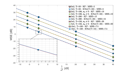
(a) kn converges to mmse.

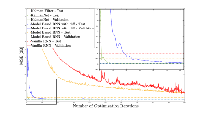
(b) Learning curves for dd se.

Figure 5: Linear ss model with full information.

IV-B2 Neural Model Selection

Next, we evaluate and confirm our design and architectural choices by considering a $2\times 2$ setup (similar to the previous one), and by comparing kn with setting C1 to two rnn based architectures of similar capacity applied for end-to-end state estimation:

• Vanilla rnn directly maps the observed $\mathbf{y}_{t}$ to an estimate of the state $\hat{\mathbf{x}}_{t}$.

• mb rnn imitates the Kalman filtering operation by first recovering $\hat{\mathbf{x}}_{t\left|t-1\right.}$ using domain knowledge, i.e., via (3a), and then uses the rnn to estimate an increment $\Delta\hat{\mathbf{x}}_{t}$ from the prior to posterior.

All rnn utilize the same architecture as in kn with a single gru layer and the same learning hyperparameters. In this experiment we test the trained models on trajectories with the same length as they were trained on, namely $T=20$. We can clearly observe how each of the key design considerations of kn affect the learning curves depicted in Fig. 5(b):

• The incorporation of the known ss model allows the mb rnn to outperform the vanilla rnn, although both converge slowly and fail to achieve the mmse.

• Using the sequences of differences as input notably improves the convergence rate of the mb rnn, indicating the benefits of using the differences as features, as discussed in Subsection III-B.

• Learning is further improved by using the rnn for recovering the kg as part of the kf flow, as done by kn, rather than for directly estimating $\mathbf{x}_{t}$.

To further evaluate the gains of kn over end-to-end rnn, we compare the pre-trained models using trajectories with different initial conditions and a longer time horizon ($T=200$) than the one on which they were trained ($T=20$). The results, summarized in Table I, show that kn maintains achieving the mmse, as already observed in Fig. 5(a). The mb rnn and vanilla rnn are more than $50\left[\textrm{dB}\right]$ from the mmse, implying that their learning is not transferable and that they do not learn to implement kfing. However, when provided with the difference features as we proposed in Subsection III-B, the dd systems are shown to be applicable in longer trajectories, with kn achieving mse within a minor gap of that achieved by the mb kf. The results of this study validate the considerations used in designing kn for the dd filtering problem discussed in Subsection II-B.

TABLE I: Test mse in [dB] when trained using $T=20$.

Test $T$	Vanilla rnn	mb rnn	mb rnn, diff.	kn	kf
$20$	-20.98	-21.53	-21.92	-21.92	-21.97
$200$	58.14	36.8	-21.88	-21.90	-21.91

IV-B3 Partial Information

To conclude our study on linear models, we next evaluate the robustness of kn to model mismatch as a result of partial model information. We simulate a $2\times 2$ ss model with mismatches in either the state-evolution model ($\mathbf{F}$) or in the state-observation model ($\mathbf{H}$).

State-Evolution Mismatch: Here, we set $T=20$ and $\nu=0\left[\textrm{dB}\right]$ and use a rotated evolution matrix $\mathbf{F}_{\alpha^{\circ}},\alpha\in\left\{10^{\circ},20^{\circ}\right\}$ for data generation. The state-evolution matrix available to the filters, denoted $\mathbf{F}_{0}$, is again set to take the controllable canonical form. The mismatched design matrix $\mathbf{F}_{0}$ is related to true $\mathbf{F}_{\alpha^{\circ}}$ via

$$\mathbf{F}_{\alpha^{\circ}}=\mathbf{R}^{\mathrm{xy}}_{\alpha^{\circ}}\cdot\mathbf{F}_{0},\quad\mathbf{R}^{\mathrm{xy}}_{\alpha^{\circ}}=\begin{pmatrix}\cos{\alpha}&-\sin{\alpha}\\ \sin{\alpha}&\cos{\alpha}\end{pmatrix}.$$ (16)

Such scenarios represent a setup in which the analytical approximation of the ss model differs from the true generative model. The resulting mse curves depicted in Fig. 6(a) demonstrate that kn (with setting C2) achieves a $3\left[\textrm{dB}\right]$ gain over the mb kf. In particular, despite the fact that kn implements the kf with an inaccurate state-evolution model, it learns to apply an alternative kg, resulting in mse within a minor gap from the mmse; i.e., from the kf with the true $\mathbf{F}_{\alpha^{\circ}}$ plugged in.

State-Observation Mismatch: Next, we simulate a setup with state-observation mismatch while setting $T=100$ and $\nu=-20\left[\textrm{dB}\right]$. The model mismatch is achieved by using a rotated observation matrix $\mathbf{H}_{\alpha=10^{\circ}}$ for data generation, while using $\mathbf{H}=\mathbf{I}$ as the observation design matrix. Such scenarios represent a setup in which a slight misalignment $(\approx 5\%)$ of the sensors exists. The resulting achieved mse depicted in Fig. 6(b) demonstrates that kn (with setting C2) converges to within a minor gap from the mmse. Here, we performed an additional experiment, first estimating the observation matrix from data, and then kn used the estimate matrix denoted $\hat{\mathbf{H}}_{\alpha}$. In this case it is observed in Fig. 6(b) that kn achieves the mmse lower bound. These results imply that kn converges also in distribution to the kf.

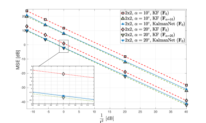
(a) State-evolution mismatch.

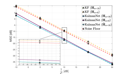
(b) State-observation mismatch.

Figure 6: Linear ss model, partial information.

IV-C Synthetic Non-Linear Model

Next, we consider a nl ss model, where the state-evolution model takes a sinusoidal form, while the state-observation model is a second order polynomial. The resulting ss model is given by

$$\mathbf{f}\left(\mathbf{x}\right) =\alpha\cdot\sin\left(\beta\cdot\mathbf{x}+\mathbf{\phi}\right)+\delta, \mathbf{x} \in\mathbb{R}^{2},$$ (17a)

$$\mathbf{h}\left(\mathbf{x}\right) =a\cdot\left(b\cdot\mathbf{x}+c\right)^{2}, \mathbf{y} \in\mathbb{R}^{2}.$$ (17b)

In the following we generate trajectories of $T=100$ time steps from the noisy ss model in (1), with $\nu=-20\left[\textrm{dB}\right]$, while using $\mathbf{f}\left(\cdot\right)$ and $\mathbf{h}\left(\cdot\right)$ as in (17) computed in a component-wise manner, with parameters as in Table II. kn is used with setting C4.

The mse values for different levels of observation noise achieved by kn compared with the mb ekf are depicted in Fig. 7 for both full and partial model information. The full evaluation with the mb ekf, ukf, and pf is given in Table III for the case of full information, and in Table IV for the case of partial information. We first observe that the ekf achieves the lowest mse values among the mb filters, therefore serving as our main mb benchmark in our experimental studies. For full information and in the low noise regime, ekf achieves the lowest mse values due to its ability to approach the mmse in such setups, and kn achieves similar performance. For higher noise levels; i.e., for $\frac{1}{\mathrm{r}^{2}}=-12.04$ [dB], the mb ekf suffers from degraded performance due to a nl effect. Nonetheless, by learning to compute the kg from data, kn manages to overcome this and achieves superior mse.

In the presence of partial model information, the state-evolution parameters used by the filters differs slightly from the true model, resulting in a notable degradation in the performance of the mb filters due to the model mismatch. In all experiments, kn overcomes such mismatches, and its performance is within a small gap of that achieved when using full information for such setups. We thus conclude that in the presence of harsh non-linearities as well as model uncertainty due to inaccurate approximation of the underlying dynamics, where mb variations of the kf fail, kn learns to approach the mmse while maintaining the rt operation and low complexity of the kf.

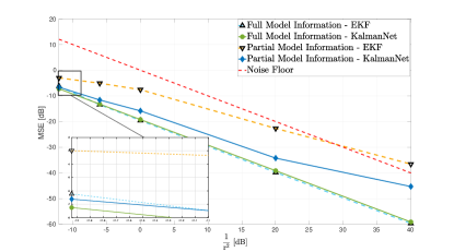
Figure 7: Non-linear ss model. kn outperforms ekf.

TABLE II: Non-linear toy problem parameters.

	$\alpha$	$\beta$	$\phi$	$\delta$	$a$	$b$	$c$
Full	$0.9$	$1.1$	$0.1\pi$	$0.01$	$1$	$1$	$0$
Partial	$1$	$1$	$0$	$0$	$1$	$1$	$0$

TABLE III: mse $\left[\textrm{dB}\right]$ – Synthetic nl ss model; full information.

${1}/{\mathrm{r}^{2}}\left[\textrm{dB}\right]$		$-12.04$	$-6.02$	$0$	$20$	$40$
ekf	$\hat{\mu}$	-6.23	-13.41	-19.58	-39.78	-59.67
	$\hat{\sigma}$	$\pm 0.89$	$\pm 0.53$	$\pm 0.47$	$\pm 0.43$	$\pm 0.44$
ukf	$\hat{\mu}$	-6.48	-13.14	-18.43	-27.24	-37.27
	$\hat{\sigma}$	$\pm 0.69$	$\pm 0.49$	$\pm 0.50$	$\pm 0.55$	$\pm 0.31$
pf	$\hat{\mu}$	-6.59	-13.33	-18.78	-26.70	-30.98
	$\hat{\sigma}$	$\pm 0.74$	$\pm 0.48$	$\pm 0.39$	$\pm 0.07$	$\pm 0.02$
kn	$\hat{\mu}$	-7.25	-13.19	-19.22	-39.13	-59.10
	$\hat{\sigma}$	$\pm 0.49$	$\pm 0.52$	$\pm 0.55$	$\pm 0.49$	$\pm 0.53$

TABLE IV: mse $\left[\textrm{dB}\right]$ – Synthetic nl ss model; partial information.

${1}/{\mathrm{r}^{2}}\left[\textrm{dB}\right]$		$-12.04$	$-6.02$	$0$	$20$	$40$
ekf	$\hat{\mu}$	-2.99	-5.07	-7.57	-22.67	-36.55
	$\hat{\sigma}$	$\pm 0.63$	$\pm 0.89$	$\pm 0.45$	$\pm 0.42$	$\pm 0.3$
ukf	$\hat{\mu}$	-0.91	-1.54	-5.18	-24.06	-37.96
	$\hat{\sigma}$	$\pm 0.60$	$\pm 0.23$	$\pm 0.29$	$\pm 0.43$	$\pm 2.21$
pf	$\hat{\mu}$	-2.32	-3.29	-4.83	-23.66	-33.13
	$\hat{\sigma}$	$\pm 0.89$	$\pm 0.53$	$\pm 0.64$	$\pm 0.48$	$\pm 0.45$
kn	$\hat{\mu}$	-6.62	-11.60	-15.83	-34.23	-45.29
	$\hat{\sigma}$	$\pm 0.46$	$\pm 0.45$	$\pm 0.44$	$\pm 0.58$	$\pm 0.64$

IV-D Lorenz Attractor

The la is a three-dimensional chaotic solution to the Lorenz system of ordinary differential equations in ct. This synthetically generated system demonstrates the task of online tracking a highly nl trajectory and a rw practical challenge of handling mismatches due to sampling a ct signal into dt [77].

In particular, the noiseless state-evolution of the ct process $\mathbf{x}_{\tau}$ with $\tau\in\mathbb{R}^{+}$ is given by

$$\frac{\partial}{\partial\tau}{\mathbf{x}}_{\tau}\!=\!\mathbf{A}\left({\mathbf{x}}_{\tau}\right)\cdot\mathbf{x}_{\tau},\hskip 2.13387pt\mathbf{A}\left({\mathbf{x}_{\tau}}\right)\!=\!\begin{pmatrix}-10&10&0\\ 28&-1&-x_{1,\tau}\\ 0&x_{1,\tau}&-\frac{8}{3}\end{pmatrix}.$$ (18)

To get a dt, state-evolution model, we repeat the steps used in [35]. First, we sample the noiseless process with sampling interval $\Delta\tau$ and assume that $\mathbf{A}\left({\mathbf{x}}_{\tau}\right)$ can be kept constant in a small neighborhood of $\mathbf{x}_{\tau}$; i.e.,

$$\mathbf{A}\left({\mathbf{x}}_{\tau}\right)\approx\mathbf{A}\left({\mathbf{x}}_{\tau+\Delta\tau}\right).$$

Then, the ct solution of the differential system (18), which is valid in the neighborhood of $\mathbf{x}_{\tau}$ for a short time interval $\Delta\tau$, is

$$\mathbf{x}_{\tau+\Delta\tau}=\exp\left(\mathbf{A}\left({\mathbf{x}_{\tau}}\right)\cdot\Delta\tau\right)\cdot\mathbf{x}_{\tau}.$$ (19)

Finally, we take the Taylor series expansion of (19) and a finite series approximation (with $J$ coefficients), which results in

$$\mathbf{F}\left({\mathbf{x}_{\tau}}\right)\triangleq\exp\left(\mathbf{A}\left({\mathbf{x}_{\tau}}\right)\cdot\Delta\tau\right)\approx\mathbf{I}+\sum_{j=1}^{J}\frac{\left(\mathbf{A}\left({\mathbf{x}_{\tau}}\right)\cdot\Delta\tau\right)^{j}}{j!}.$$ (20)

The resulting dt evolution process is given by

$$\mathbf{x}_{t+1}=\mathbf{f}\left(\mathbf{x}_{t}\right)=\mathbf{F}\left({\mathbf{x}_{t}}\right)\cdot\mathbf{x}_{t}.$$ (21)

The dt state-evolution model in (21), with additional process noise, is used for generating the simulated la data. Unless stated otherwise the data was generated with $J=5$ Taylor order and $\Delta\tau=0.02$ sampling interval. In the following experiments, kn is consistently invariant of the distribution of the noise signals, with the models it uses for $\mathbf{f}\left(\cdot\right)$ and $\mathbf{h}\left(\cdot\right)$ varying between the different studies, as discussed in the sequel.

IV-D1 Full Information

We first compare kn to the mb filter when using the state-evolution matrix $\mathbf{F}$ computed via (20) with $J=5$.

Noisy state observations: Here, we set $\mathbf{h}\left(\cdot\right)$ to be the identity transformation, such that the observations are noisy versions of the true state. Further, we set $\nu=-20\left[\textrm{dB}\right]$ and $T=2000$. As observed in Fig. 8(a), despite being trained on short trajectories $T=100$, kn (with setting C3) achieves excellent mse performance—namely, comparable to ekf—and outperforms the ukf and pf. The full details of the experiment are given in Table V. All the mb algorithms were optimized for performance; e.g., applying the ekf with full model information achieves an unstable state tracking performance, with mse values surpassing $30\left[\textrm{dB}\right]$. To stabilize the ekf, we had to perform a grid search using the available data set to optimize the process noise $\mathbf{Q}$ used by the filter.

TABLE V: mse $\left[\textrm{dB}\right]$ – la with noisy state observations.

${1}/{\mathrm{r}^{2}}\left[\textrm{dB}\right]$	$0$	$10$	$20$	$30$	$40$
ekf	-10.45	-20.37	-30.40	-40.39	-49.89
ukf	-5.62	-12.04	-20.45	-30.05	-40.00
pf	-9.78	-18.13	-23.54	-30.16	-33.95
kn	-9.79	-19.75	-29.37	-39.68	-48.99

Noisy nl observations: Next, we consider the case where the observations are given by a non-linear function of the current state, setting $\mathbf{h}$ to take the form of a transformation from a cartesian coordinate system to spherical coordinates. We further set $T=20$ and $\nu=0\left[\textrm{dB}\right]$. From the results depicted in Fig. 8(b) and reported in Table VI we observe that in such non-linear setups, the sub-optimal mb approaches operating with full information of the ss model are substantially outperformed by kn (with setting C4).

TABLE VI: mse $\left[\textrm{dB}\right]$ – la with non-linear observations

${1}/{\mathrm{r}^{2}}\left[\textrm{dB}\right]$	$-10$	$0$	$10$	$20$	$30$
ekf	26.38	21.78	14.50	4.84	-4.02
ukf	nan	nan	nan	nan	nan
pf	24.85	20.91	14.23	11.93	4.35
kn	14.55	6.77	-1.77	-10.57	-15.24

(a) $T=2000$, $\nu=-20\left[\textrm{dB}\right]$, $\mathbf{h}\left(\cdot\right)=\mathbf{I}$.

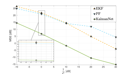
(b) $T=20$, $\nu=0\left[\textrm{dB}\right]$, $\mathbf{h}\left(\cdot\right)$ nl.

Figure 8: la, full information.

IV-D2 Partial Information

W proceed to evaluate kn and compare it to its mb counterparts under partial model information. We consider three possible sources of model mismatch arising in the la setup:

• State-evolution mismatch due to use of a Taylor series approximation of insufficient order.

• State-observation mismatch as a result of misalignment due to rotation.

• State-observation mismatch as a result of sampling from ct to dt.

Since the ekf produced the best results in the full information case among all nl mb filtering algorithms, we use it as a baseline for the mse lower bound.

State-evolution mismatch: In this study, both kn and the mb algorithms operate with a crude approximation of the evolution dynamics obtained by computing (20) with $J=2$, while the data is generated with an order $J=5$ Taylor series expansion. We again set $\mathbf{h}$ to be the identity mapping, $T=2000$, and $\nu=-20\left[\textrm{dB}\right]$. The results, depicted in Fig. 9(a) and reported in Table VII, demonstrate that kn (with setting C4) learns to partially overcome this model mismatch, outperforming its mb counterparts operating with the same level of partial information.

TABLE VII: mse $\left[\textrm{dB}\right]$ - la with state-evolution mismatch $J=2$.

${1}/{\mathrm{r}^{2}}\left[\textrm{dB}\right]$		$10$	$20$	$30$	$40$
ekf	$\hat{\mu}$	-20.37	-30.40	-40.39	-49.89
$J=5$	$\hat{\sigma}$	$\pm 0.25$	$\pm 0.24$	$\pm 0.24$	$\pm 0.20$
ekf	$\hat{\mu}$	-19.47	-23.63	-33.51	-41.15
$J=2$	$\hat{\sigma}$	$\pm 0.25$	$\pm 0.11$	$\pm 0.18$	$\pm 0.12$
ukf	$\hat{\mu}$	-11.95	-20.45	-30.05	-39.98
$J=2$	$\hat{\sigma}$	$\pm 0.87$	$\pm 0.27$	$\pm 0.09$	$\pm 0.09$
pf	$\hat{\mu}$	-17.95	-23.47	-30.11	-33.81
$J=2$	$\hat{\sigma}$	$\pm 0.18$	$\pm 0.09$	$\pm 0.10$	$\pm 0.13$
kn	$\hat{\mu}$	-19.71	-27.07	-35.41	-41.74
$J=2$	$\hat{\sigma}$	$\pm 0.29$	$\pm 0.18$	$\pm 0.20$	$\pm 0.11$

State-observation rotation mismatch: Here, the presence of mismatch in the observations model is simulated by using data generated by an identity matrix rotated by merely $\theta=1^{\circ}$. This rotation is equivalent to sensor misalignment of $\approx 0.55\%$. The results depicted in Figure. 9(b) and reported in Table VIII clearly demonstrate that this seemingly minor rotation can cause a severe performance degradation for the mb filters, while kn (with setting C3) is able to learn from data to overcome such mismatches and to notably outperform its mb counterparts, which are sensitive to model uncertainty. Here, we trained kn on short trajectories with $T=100$ time steps, tested it on longer trajectories with $T=1000$ time steps, and set $\nu=-20\left[\textrm{dB}\right]$. This again demonstrates that the learning of kn is transferable.

TABLE VIII: mse $\left[\textrm{dB}\right]$ - la with observation rotation.

${1}/{\mathrm{r}^{2}}\left[\textrm{dB}\right]$		$0$	$10$	$20$	$30$
ekf	$\hat{\mu}$	-10.40	-20.41	-30.50	-40.45
$\theta=0^{\circ}$	$\hat{\sigma}$	$\pm 0.35$	$\pm 0.37$	$\pm 0.34$	$\pm 0.34$
ekf	$\hat{\mu}$	-9.80	-16.50	-18.19	-18.57
$\theta=1^{\circ}$	$\hat{\sigma}$	$\pm 0.54$	$\pm 6.51$	$\pm 0.22$	$\pm 0.21$
ukf	$\hat{\mu}$	-2.08	-6.92	-7.89	-8.09
$\theta=1^{\circ}$	$\hat{\sigma}$	$\pm 1.73$	$\pm 0.53$	$\pm 0.59$	$\pm 0.62$
pf	$\hat{\mu}$	-8.48	-0.18	15.24	19.87
$\theta=1^{\circ}$	$\hat{\sigma}$	$\pm 3$	$\pm 8.21$	$\pm 3.50$	$\pm 0.80$
kn	$\hat{\mu}$	-9.63	-18.17	-27.32	-34.04
$\theta=1^{\circ}$	$\hat{\sigma}$	$\pm 0.53$	$\pm 0.42$	$\pm 0.67$	$\pm 0.77$

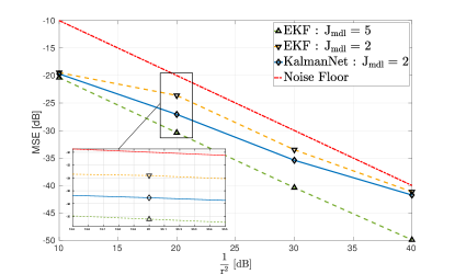
(a) State-evolution mismatch, identity $\mathbf{h}$, $T=2000$.

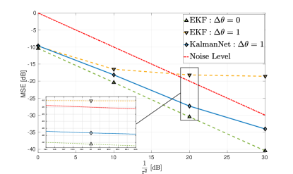
(b) Observation mismatch - $\Delta\theta=1^{\circ}$, $T=1000$.

Figure 9: la, partial information.

State-observations sampling mismatch: We conclude our experimental study of the la setup with an evaluation of kn in the presence of sampling mismatch. Here, we generate data from the la ss model with an approximate ct evolution process using a dense sampling rate, set to ${\Delta\tau=10^{-5}}$. We then sub-sample the noiseless observations from the evolution process by a ratio of $\frac{1}{2000}$ and get a decimated process with $\Delta\tau_{\textrm{d}}=0.02$. This procedure results in an inherent mismatch in the ss model due to representing an (approximately) ct process using a dt sequence. In this experiment, no process noise was applied, and the observations are again obtained with $\mathbf{h}$ set to identity and $T=3000$.

The resulting mse values for $\frac{1}{\mathrm{r}^{2}}=0\left[\textrm{dB}\right]$ of kn with configuration C4 compared with the mb filters and with the end-to-end neural network termed mb-rnn (see Subsection IV-B) are reported in Table IX. The results demonstrate that kn overcomes the mismatch induced by representing a ct ss model in dt, achieving a substantial processing gain over the mb alternatives due to its learning capabilities. The results also demonstrate that kn significantly outperforms a straightforward combination of domain knowledge; i.e. a state-transition function $\mathbf{f}\left(\cdot\right)$, with end-to-end rnn. A fully model-agnostic rnn was shown to diverge when trained for this task. In Fig. 10 we visualize how this gain is translated into clearly improved tracking of a single trajectory. To show that these gains of kn do not come at the cost of computationally slow inference, we detail the average inference time for all filters (without parallelism). The stopwatch timings were measured on the same platform – Google Colab with CPU: Intel(R) Xeon(R) CPU @ 2.20GHz, GPU: Tesla P100-PCIE-16GB. We see that kn infers faster than the classical methods, thanks to the highly efficient neural network computations and the fact that, unlike the mb filters, it does not involve linearization and matrix inversions for each time step.

TABLE IX: la with sampling mismatch.

Metric	ekf	ukf	pf	kn	mb-rnn
mse $\left[\textrm{dB}\right]$	-6.432	-5.683	-5.337	-11.284	17.355
$\hat{\sigma}$	$\pm 0.093$	$\pm 0.166$	$\pm 0.190$	$\pm 0.301$	$\pm 0.527$
Run-time $[\sec]$	5.440	6.072	62.946	4.699	2.291

IV-E Real World Dynamics: Michigan NCLT Data Set

In our final experiment we evaluate kn on the Michigan nclt ds [28]. This ds comprises different labeled trajectories, with each one containing noisy sensor readings (e.g., GPS and odometer) and the ground truth locations of a moving Segway robot. Given these noisy readings, the goal of the tracking algorithm is to localize the Segway from the raw measurements at any given time.

To tackle this problem we model the Segway kinematics (in each axis separately) using the linear Wiener velocity model, where the acceleration is modeled as a white Gaussian noise process $w_{\tau}$ with variance $\mathrm{q}^{2}$ [36]:

$$\mathbf{x}_{\tau}=\left(p,v\right)^{\top}\in\mathbb{R}^{2},\quad\frac{\partial}{\partial\tau}{\mathbf{x}}_{\tau}=\begin{pmatrix}0&1\\ 0&0\end{pmatrix}\cdot\mathbf{x}_{\tau}+\begin{pmatrix}0\\ w_{\tau}\end{pmatrix}.$$ (22)

Here, $p$ and $v$ are the position and velocity, respectively. The dt state-evolution with sampling interval $\Delta\tau$ is approximated as a linear ss model in which the evolution matrix $\mathbf{F}$ and noise covariance $\mathbf{Q}$ are given by

$$\mathbf{F}=\begin{pmatrix}1&\Delta\tau\\ 0&1\end{pmatrix},\quad\mathbf{Q}={\color[rgb]{0,0,0}\mathrm{q}^{2}}\cdot\begin{pmatrix}\frac{1}{3}\cdot\left(\Delta\tau\right)^{3}&\frac{1}{2}\cdot\left(\Delta\tau\right)^{2}\\ \frac{1}{2}\cdot\left(\Delta\tau\right)^{2}&\Delta\tau\end{pmatrix}.$$ (23)

Since kn does not rely on knowledge of the noise covariance matrices, $\mathbf{Q}$ is given here for the use of the mb kf and for completeness.

The goal is to track the underlying state vector in both axes solely using odometry data; i.e., the observations are given by noisy velocity readings. In this case the observations obey a noisy linear model:

$$\mathrm{y}\in\mathbb{R},\quad\mathbf{H}=\left(0,1\right).$$ (24)

Such settings where one does not have access to direct measurements for positioning are very challenging yet practical and typical for many applications where positioning technologies are not available indoors, and one must rely on noisy odometer readings for self-localization. Odometry-based estimated positions typically start drifting away at some point.

In the assumed model, the x-axis (in cartesian coordinates) are decoupled from the y-axis, and the linear ss model used for Kalman filtering is given by

$$\tilde{\mathbf{F}} =\begin{pmatrix}\mathbf{F}&0\\ 0&\mathbf{F}\end{pmatrix}\in\mathbb{R}^{4\times 4},\quad\tilde{\mathbf{Q}}=\begin{pmatrix}\mathbf{Q}&0\\ 0&\mathbf{Q}\end{pmatrix}\in\mathbb{R}^{4\times 4},$$ (25a)

$$\tilde{\mathbf{H}} =\begin{pmatrix}\mathbf{H}&0\\ 0&\mathbf{H}\end{pmatrix}\in\mathbb{R}^{2\times 4},\quad\tilde{\mathbf{R}}=\begin{pmatrix}\mathrm{r}^{2}&0\\ 0&\mathrm{r^{2}}\end{pmatrix}\in\mathbb{R}^{2\times 2}.$$ (25b)

This model is equivalent to applying two independent kf in parallel. Unlike the mb kf, kn does not rely on noise modeling, and can thus accommodate dependency in its learned kg.

We arbitrarily use the session with date 2012-01-22 that consists of a single trajectory. Sampling at $1\textrm{[Hz]}$ results in $5,850$ time steps. We removed unstable readings and were left with 5,556 time steps. The trajectory was split into three sections: $85\%$ for training ($23$ sequences of length $T=200$), $10\%$ for validation ($2$ sequences, $T=200$), and $5\%$ for testing ($1$ sequence, $T=277$). We compare kn with setting C1 to end-to-end vanilla rnn and the mb kf, where for the latter the matrices $\mathbf{Q}$ and $\mathbf{R}$ were optimized through a grid search.

Fig. 11 and Table X demonstrate the superiority of kn for such scenarios. kf blindly follows the odometer trajectory and is incapable of accounting for the drift, producing a very similar or even worse estimation than the integrated velocity. The vanilla rnn, which is agnostic of the motion model, fails to localize. kn overcomes the errors induced by the noisy odometer observations, and provides the most accurate rt locations, demonstrating the gains of combining mb kf-based inference with integrated dd modules for rw applications.

TABLE X: Numerical mse $\left[\textrm{dB}\right]$ for the NCLT experiment.

Baseline	ekf	kn	Vanilla RNN
25.47	25.385	22.2	40.21

Figure 10: la with sampling mismatch (decimation), $T=3000$.

Figure 11: NCLT ds: ground truth vs. integrated velocity, trajectory from session with date 2012-01-22 sampled at 1 Hz.

V Conclusions

In this work we presented kn, a hybrid combination of dl with the classic mb ekf. Our design identifies the ss-model-dependent computations of the mb ekf, replacing them with a dedicated rnn operating on specific features encapsulating the information needed for its operation. Our numerical study shows that doing so enables kn to carry out rt se in the same manner as mb Kalman filtering, while learning to overcome model mismatches and non-linearities. kn uses a relatively compact rnn that can be trained with a relatively small ds and infers a reduced complexity, making it applicable for high dimensional ss models and computationally limited devices.

References

- [1] G. Revach, N. Shlezinger, R. J. G. van Sloun, and Y. C. Eldar, “KalmanNet: Data-driven Kalman filtering,” in Proc. IEEE ICASSP, 2021, pp. 3905–3909.
- [2] J. Durbin and S. J. Koopman, Time series analysis by state space methods. Oxford University Press, 2012.
- [3] R. E. Kalman, “A new approach to linear filtering and prediction problems,” Journal of Basic Engineering, vol. 82, no. 1, pp. 35–45, 1960.
- [4] R. E. Kalman and R. S. Bucy, “New results in linear filtering and prediction theory,” 1961.
- [5] R. E. Kalman, “New methods in Wiener filtering theory,” 1963.
- [6] N. Wiener, Extrapolation, interpolation, and smoothing of stationary time series: With engineering applications. MIT Press Cambridge, MA, 1949, vol. 8.
- [7] M. Gruber, “An approach to target tracking,” MIT Lexington Lincoln Lab, Tech. Rep., 1967.
- [8] R. E. Larson, R. M. Dressler, and R. S. Ratner, “Application of the Extended Kalman filter to ballistic trajectory estimation,” Stanford Research Institute, Tech. Rep., 1967.
- [9] J. D. McLean, S. F. Schmidt, and L. A. McGee, Optimal filtering and linear prediction applied to a midcourse navigation system for the circumlunar mission. National Aeronautics and Space Administration, 1962.
- [10] S. J. Julier and J. K. Uhlmann, “New extension of the Kalman filter to nonlinear systems,” in Signal Processing, Sensor Fusion, and Target Recognition VI, vol. 3068. International Society for Optics and Photonics, 1997, pp. 182–193.
- [11] N. J. Gordon, D. J. Salmond, and A. F. Smith, “Novel approach to nonlinear/non-Gaussian Bayesian state estimation,” in IEE proceedings F (radar and signal processing), vol. 140, no. 2. IET, 1993, pp. 107–113.
- [12] P. Del Moral, “Nonlinear filtering: Interacting particle resolution,” Comptes Rendus de l’Académie des Sciences-Series I-Mathematics, vol. 325, no. 6, pp. 653–658, 1997.
- [13] J. S. Liu and R. Chen, “Sequential Monte Carlo methods for dynamic systems,” Journal of the American Statistical Association, vol. 93, no. 443, pp. 1032–1044, 1998.
- [14] F. Auger, M. Hilairet, J. M. Guerrero, E. Monmasson, T. Orlowska-Kowalska, and S. Katsura, “Industrial applications of the Kalman filter: A review,” IEEE Trans. Ind. Electron., vol. 60, no. 12, pp. 5458–5471, 2013.
- [15] M. Zorzi, “Robust Kalman filtering under model perturbations,” IEEE Trans. Autom. Control, vol. 62, no. 6, pp. 2902–2907, 2016.
- [16] ——, “On the robustness of the Bayes and Wiener estimators under model uncertainty,” Automatica, vol. 83, pp. 133–140, 2017.
- [17] A. Longhini, M. Perbellini, S. Gottardi, S. Yi, H. Liu, and M. Zorzi, “Learning the tuned liquid damper dynamics by means of a robust EKF,” arXiv preprint arXiv:2103.03520, 2021.
- [18] Y. LeCun, Y. Bengio, and G. Hinton, “Deep learning,” Nature, vol. 521, no. 7553, p. 436, 2015.
- [19] Y. Bengio, “Learning deep architectures for AI,” Foundations and Trends® in Machine Learning, vol. 2, no. 1, pp. 1–127, 2009.
- [20] S. Hochreiter and J. Schmidhuber, “Long short-term memory,” Neural Computation, vol. 9, no. 8, pp. 1735–1780, 1997.
- [21] J. Chung, C. Gulcehre, K. Cho, and Y. Bengio, “Empirical evaluation of gated recurrent neural networks on sequence modeling,” arXiv preprint arXiv:1412.3555, 2014.
- [22] A. Vaswani, N. Shazeer, N. Parmar, J. Uszkoreit, L. Jones, A. N. Gomez, L. Kaiser, and I. Polosukhin, “Attention is all you need,” arXiv preprint arXiv:1706.03762, 2017.
- [23] M. Zaheer, A. Ahmed, and A. J. Smola, “Latent LSTM allocation: Joint clustering and non-linear dynamic modeling of sequence data,” in International Conference on Machine Learning, 2017, pp. 3967–3976.
- [24] N. Shlezinger, N. Farsad, Y. C. Eldar, and A. J. Goldsmith, “ViterbiNet: A deep learning based Viterbi algorithm for symbol detection,” IEEE Trans. Wireless Commun., vol. 19, no. 5, pp. 3319–3331, 2020.
- [25] N. Shlezinger, R. Fu, and Y. C. Eldar, “DeepSIC: Deep soft interference cancellation for multiuser MIMO detection,” IEEE Trans. Wireless Commun., vol. 20, no. 2, pp. 1349–1362, 2021.
- [26] N. Shlezinger, N. Farsad, Y. C. Eldar, and A. J. Goldsmith, “Learned factor graphs for inference from stationary time sequences,” IEEE Trans. Signal Process., early access, 2022.
- [27] N. Shlezinger, J. Whang, Y. C. Eldar, and A. G. Dimakis, “Model-based deep learning,” arXiv preprint arXiv:2012.08405, 2020.
- [28] N. Carlevaris-Bianco, A. K. Ushani, and R. M. Eustice, “University of Michigan North Campus long-term vision and LiDAR dataset,” The International Journal of Robotics Research, vol. 35, no. 9, pp. 1023–1035, 2016.
- [29] R. G. Krishnan, U. Shalit, and D. Sontag, “Deep Kalman filters,” arXiv preprint arXiv:1511.05121, 2015.
- [30] M. Karl, M. Soelch, J. Bayer, and P. Van der Smagt, “Deep variational Bayes filters: Unsupervised learning of state space models from raw data,” arXiv preprint arXiv:1605.06432, 2016.
- [31] M. Fraccaro, S. D. Kamronn, U. Paquet, and O. Winther, “A disentangled recognition and nonlinear dynamics model for unsupervised learning,” in Advances in Neural Information Processing Systems, 2017.
- [32] C. Naesseth, S. Linderman, R. Ranganath, and D. Blei, “Variational sequential Monte Carlo,” in International Conference on Artificial Intelligence and Statistics. PMLR, 2018, pp. 968–977.
- [33] E. Archer, I. M. Park, L. Buesing, J. Cunningham, and L. Paninski, “Black box variational inference for state space models,” arXiv preprint arXiv:1511.07367, 2015.
- [34] R. Krishnan, U. Shalit, and D. Sontag, “Structured inference networks for nonlinear state space models,” in Proceedings of the AAAI Conference on Artificial Intelligence, vol. 31, no. 1, 2017.
- [35] V. G. Satorras, Z. Akata, and M. Welling, “Combining generative and discriminative models for hybrid inference,” in Advances in Neural Information Processing Systems, 2019, pp. 13 802–13 812.
- [36] Y. Bar-Shalom, X. R. Li, and T. Kirubarajan, Estimation with applications to tracking and navigation: Theory algorithms and software. John Wiley & Sons, 2004.
- [37] K.-V. Yuen and S.-C. Kuok, “Online updating and uncertainty quantification using nonstationary output-only measurement,” Mechanical Systems and Signal Processing, vol. 66, pp. 62–77, 2016.
- [38] H.-Q. Mu, S.-C. Kuok, and K.-V. Yuen, “Stable robust Extended Kalman filter,” Journal of Aerospace Engineering, vol. 30, no. 2, p. B4016010, 2017.
- [39] I. Arasaratnam, S. Haykin, and R. J. Elliott, “Discrete-time nonlinear filtering algorithms using Gauss–Hermite quadrature,” Proc. IEEE, vol. 95, no. 5, pp. 953–977, 2007.
- [40] I. Arasaratnam and S. Haykin, “Cubature Kalman filters,” IEEE Trans. Autom. Control, vol. 54, no. 6, pp. 1254–1269, 2009.
- [41] M. S. Arulampalam, S. Maskell, N. Gordon, and T. Clapp, “A tutorial on particle filters for online nonlinear/non-Gaussian Bayesian tracking,” IEEE Trans. Signal Process., vol. 50, no. 2, pp. 174–188, 2002.
- [42] N. Chopin, P. E. Jacob, and O. Papaspiliopoulos, “SMC2: An efficient algorithm for sequential analysis of state space models,” Journal of the Royal Statistical Society: Series B (Statistical Methodology), vol. 75, no. 3, pp. 397–426, 2013.
- [43] L. Martino, V. Elvira, and G. Camps-Valls, “Distributed particle metropolis-Hastings schemes,” in IEEE Statistical Signal Processing Workshop (SSP), 2018, pp. 553–557.
- [44] C. Andrieu, A. Doucet, and R. Holenstein, “Particle Markov chain Monte Carlo methods,” Journal of the Royal Statistical Society: Series B (Statistical Methodology), vol. 72, no. 3, pp. 269–342, 2010.
- [45] J. Elfring, E. Torta, and R. van de Molengraft, “Particle filters: A hands-on tutorial,” Sensors, vol. 21, no. 2, p. 438, 2021.
- [46] R. H. Shumway and D. S. Stoffer, “An approach to time series smoothing and forecasting using the EM algorithm,” Journal of Time Series Analysis, vol. 3, no. 4, pp. 253–264, 1982.
- [47] Z. Ghahramani and G. E. Hinton, “Parameter estimation for linear dynamical systems,” 1996.
- [48] J. Dauwels, A. Eckford, S. Korl, and H.-A. Loeliger, “Expectation maximization as message passing-part I: Principles and Gaussian messages,” arXiv preprint arXiv:0910.2832, 2009.
- [49] L. Martino, J. Read, V. Elvira, and F. Louzada, “Cooperative parallel particle filters for online model selection and applications to urban mobility,” Digital Signal Processing, vol. 60, pp. 172–185, 2017.
- [50] P. Abbeel, A. Coates, M. Montemerlo, A. Y. Ng, and S. Thrun, “Discriminative training of Kalman filters.” in Robotics: Science and Systems, vol. 2, 2005, p. 1.
- [51] L. Xu and R. Niu, “EKFNet: Learning system noise statistics from measurement data,” in Proc. IEEE ICASSP, 2021, pp. 4560–4564.
- [52] S. T. Barratt and S. P. Boyd, “Fitting a Kalman smoother to data,” in IEEE American Control Conference (ACC), 2020, pp. 1526–1531.
- [53] L. Xie, Y. C. Soh, and C. E. De Souza, “Robust Kalman filtering for uncertain discrete-time systems,” IEEE Trans. Autom. Control, vol. 39, no. 6, pp. 1310–1314, 1994.
- [54] C. M. Carvalho, M. S. Johannes, H. F. Lopes, and N. G. Polson, “Particle learning and smoothing,” Statistical Science, vol. 25, no. 1, pp. 88–106, 2010.
- [55] I. Urteaga, M. F. Bugallo, and P. M. Djurić, “Sequential Monte Carlo methods under model uncertainty,” in IEEE Statistical Signal Processing Workshop (SSP), 2016, pp. 1–5.
- [56] L. Zhou, Z. Luo, T. Shen, J. Zhang, M. Zhen, Y. Yao, T. Fang, and L. Quan, “KFNet: Learning temporal camera relocalization using Kalman filtering,” in Proceedings of the IEEE/CVF Conference on Computer Vision and Pattern Recognition, 2020, pp. 4919–4928.
- [57] D. P. Kingma and M. Welling, “Auto-encoding variational Bayes,” arXiv preprint arXiv:1312.6114, 2013.
- [58] D. J. Rezende, S. Mohamed, and D. Wierstra, “Stochastic backpropagation and approximate inference in deep generative models,” in International conference on machine learning. PMLR, 2014, pp. 1278–1286.
- [59] D. M. Blei, A. Kucukelbir, and J. D. McAuliffe, “Variational inference: A review for statisticians,” Journal of the American Statistical Association, vol. 112, no. 518, pp. 859–877, 2017.
- [60] T. Haarnoja, A. Ajay, S. Levine, and P. Abbeel, “Backprop kf: Learning discriminative deterministic state estimators,” in Advances in Neural Information Processing Systems, 2016, pp. 4376–4384.
- [61] B. Laufer-Goldshtein, R. Talmon, and S. Gannot, “A hybrid approach for speaker tracking based on TDOA and data-driven models,” IEEE/ACM Trans. Audio, Speech, Language Process., vol. 26, no. 4, pp. 725–735, 2018.
- [62] H. Coskun, F. Achilles, R. DiPietro, N. Navab, and F. Tombari, “Long short-term memory Kalman filters: Recurrent neural estimators for pose regularization,” in Proceedings of the IEEE International Conference on Computer Vision, 2017, pp. 5524–5532.
- [63] S. S. Rangapuram, M. W. Seeger, J. Gasthaus, L. Stella, Y. Wang, and T. Januschowski, “Deep state space models for time series forecasting,” in Advances in Neural Information Processing Systems, 2018, pp. 7785–7794.
- [64] P. Becker, H. Pandya, G. Gebhardt, C. Zhao, C. J. Taylor, and G. Neumann, “Recurrent Kalman networks: Factorized inference in high-dimensional deep feature spaces,” in International Conference on Machine Learning. PMLR, 2019, pp. 544–552.
- [65] X. Zheng, M. Zaheer, A. Ahmed, Y. Wang, E. P. Xing, and A. J. Smola, “State space LSTM models with particle MCMC inference,” arXiv preprint arXiv:1711.11179, 2017.
- [66] T. Salimans, D. Kingma, and M. Welling, “Markov chain Monte Carlo and variational inference: Bridging the gap,” in International Conference on Machine Learning. PMLR, 2015, pp. 1218–1226.
- [67] X. Ni, G. Revach, N. Shlezinger, R. J. van Sloun, and Y. C. Eldar, “RTSNET: Deep learning aided Kalman smoothing,” in Proc. IEEE ICASSP, 2022.
- [68] R. Dey and F. M. Salem, “Gate-variants of gated recurrent unit (GRU) neural networks,” in Proc. IEEE MWSCAS, 2017, pp. 1597–1600.
- [69] P. J. Werbos, “Backpropagation through time: What it does and how to do it,” Proc. IEEE, vol. 78, no. 10, pp. 1550–1560, 1990.
- [70] I. Sutskever, Training recurrent neural networks. University of Toronto Toronto, Canada, 2013.
- [71] I. Klein, G. Revach, N. Shlezinger, J. E. Mehr, R. J. van Sloun, and Y. Eldar, “Uncertainty in data-driven Kalman filtering for partially known state-space models,” in Proc. IEEE ICASSP, 2022.
- [72] A. López Escoriza, G. Revach, N. Shlezinger, and R. J. G. van Sloun, “Data-driven Kalman-based velocity estimation for autonomous racing,” in Proc. IEEE ICAS, 2021.
- [73] H. E. Rauch, F. Tung, and C. T. Striebel, “Maximum likelihood estimates of linear dynamic systems,” AIAA Journal, vol. 3, no. 8, pp. 1445–1450, 1965.
- [74] D. P. Kingma and J. Ba, “Adam: A method for stochastic optimization,” arXiv preprint arXiv:1412.6980, 2014.
- [75] Labbe, Roger, FilterPy - Kalman and Bayesian Filters in Python, 2020. [Online]. Available: https://filterpy.readthedocs.io/en/latest/
- [76] Jerker Nordh, pyParticleEst - Particle based methods in Python, 2015. [Online]. Available: https://pyparticleest.readthedocs.io/en/latest/index.html
- [77] W. Gilpin, “Chaos as an interpretable benchmark for forecasting and data-driven modelling,” arXiv preprint arXiv:2110.05266, 2021.