MSC Classification: 41A10, 41A52, 65D15

Keywords: Approximation, error bounds, uniqueness, stability, alternation, radial basis functions, kernels, reproducing kernel Hilbert spaces, duality.

Abstract: The concept of $H$-sets as introduced by Collatz in 1956 was very useful in univariate Chebyshev approximation by polynomials or Chebyshev spaces. In the multivariate setting, the situation is much worse, because there is no alternation, and $H$-sets exist, but are only rarely accessible by mathematical arguments. However, in Reproducing Kernel Hilbert spaces, $H$-sets are shown here to have a rather simple and complete characterization. As a byproduct, the strong connection of $H$-sets to Linear Programming is studied. But on the downside, it is explained why $H$-sets have a very limited range of applicability in the times of large-scale computing.

1 $H$-Sets and Their Use

Let $F$ be a space of continuous real-valued functions on a compact domain $T$, and consider linear approximations of functions $f$ by functions $v$ from a subspace $V$ of $F$. In 1956, Lothar Collatz [4] introduced

Definition 1.

An $H$-set for $V\subseteq F\subseteq C(T)$ consists of a subset $H$ of $T$ and a sign function $\sigma\;:\;H\to\{-1,+1\}$ such that there is no $v\in V$ that makes all values $v(h)\sigma(h)$ for $h\in H$ negative.

The classical application is in linear Chebyshev approximation [4], stated here in abstract form:

Theorem 1.

Assume that a user has found some candidate $\tilde{v}\in V$ for approximation of $f\in F$ by functions from $V$, and an $H$-set consisting of $H$ and $\sigma$. If furthermore

$$\inf_{h\in H}(f(h)-\tilde{v}(h))\sigma(h)=:\mu$$ (1)

is positive, then

$$\mu\leq\displaystyle{\inf_{v\in V}\|f-v\|_{\infty}}\leq\|f-\tilde{v}\|_{\infty}$$

bounds the optimal approximation error from both sides by observable quantities.

Proof: For any $v\in V$, the expression

$$\begin{array}[]{rcl}\|f-v\|_{\infty}&\geq&(f(h)-v(h))\sigma(h)\\ &=&(f(h)-\tilde{v}(h))\sigma(h)+(\tilde{v}(h)-v(h))\sigma(h)\\ \end{array}$$

implies

$$\|f-v\|_{\infty}\geq(f(\tilde{h})-\tilde{v}(\tilde{h}))\sigma(\tilde{h})\geq\mu$$

for some $\tilde{h}\in H$. $\Box$

This shows that $H$-sets should pick near-extremal points of the error function and keep the sign of the error there. In 1956, computations were still made mechanically, and then $H$-sets allowed to assess the quality of an approximation without any large-scale computation.

If $H$ has only $N$ points, if $V$ is $n$-dimensional, and if the corresponding discrete Chebyshev approximation on $H$ is carried out exactly by a linear optimizer of Simplex type, one gets an $H$-set based on extremal points for free, as we shall prove in Theorem 3 below. However, Theorem 1 is useless in that case, because best approximation errors on $T$ always have lower bounds by best approximation errors on subsets. This implies that the merits of specially constructed $H$-sets are restricted to inexact discrete Chebyshev approximation.

2 Examples

The simplest and classical example is Chebyshev approximation in $C[-1,+1]$ by polynomials of degree $n$. One can expect alternation of the error of best Chevyshev approximations on sets $T$ of $n+2$ points, and these are the canonical candidates for an $H$ set, the signs being alternating wrt. the ordering of the points. The Remes exchange algorithm makes heavy use of this principle, and Theorem 1 can be applied as soon as sign patterns and extremal points stabilize in the iteration.

For multivariate approximation, there is no alternation principle, and $H$-sets may be very hard to determine. But we shall see in section 4 that this is not the case for kernel-based spaces.

In general, after performing some numerical approximation, one may choose near-extremal points, with signs related to the sign of the error there to get a candidate for an $H$-set, satisfying (1), but then one must hope for the $H$-set property for that choice of signs.

Conversely, one might prove the $H$-set property for a fixed choice of $V$, $H$, and $\sigma$, but then the application requires these signs to arise in (1), limiting the applicability seriously.

This gap is a general obstacle to the practical applicability of $H$-sets.

3 Connections to Linear Optimization

It is strange that most of the literature on $H$-sets (see e.g. Taylor [9], Brannigan [1], Dierieck [5], and Brannigan [2]) focuses on minimality and geometry of $H$-sets and has some links to duality, but no explicit connection to Linear Optimization. The only exception seems to be Wetterling [11] who briefly mentions the connection of $H$-sets to the dual Simplex algorithm. We give details here, to prepare for the kernel-based case.

If $V$ is $n$-dimensional with basis $v_{1},\ldots,v_{n}$ and if $H$ has $N$ points $h_{1},\ldots,h_{N}$ with associated signs $\sigma_{1},\ldots,\sigma_{N}$, one can form the $N\times n$ matrix $A$ with entries $v_{i}(h_{k})\sigma_{k}$.

Theorem 2.

Under the above notation, the $H$-set property is equivalent to the two equivalent dual statements:

• There is no $x\in\mathbb{R}^{n}$ such that the vector $b:=Ax\in\mathbb{R}^{N}$ is negative in all components,

• There is a nonzero nonnegative vector $w\in\mathbb{R}^{N}$ with

  $$w^{T}A=0=\sum_{k=1}^{N}w_{k}v_{i}(h_{k})\sigma_{k},\;1\leq i\leq n.$$ (2)

Proof: The first statement is the definition of the $H$-set property. The second implies the first, because $w^{T}Ax=0=w^{T}b$ makes it impossible that $b:=Ax\in\mathbb{R}^{N}$ is negative in all components. The converse is also true, due to the Farkas lemma in the background:

• $Ax\leq b$ is solvable if and only if for all vectors $w\geq 0$ and $w^{T}A=0$ the inequality $w^{T}b\geq 0$ holds.

If we have an $H$-set, the problem $Ax\leq-\beta 1$ is unsolvable for small fixed $\beta>0$. This implies that $Ax\leq-1$ is unsolvable, and then there is a $w\geq 0$ with $w^{T}A=0$ and $-1^{T}w<0$. $\Box$

We shall use (2) for a numerical test for the $H$-set property. To decide that $H$ and $\sigma$ form an $H$-set or not, we pose the solvable problem

$$\begin{array}[]{rcl}1^{T}w&=&Max!\\ 0\leq&w&\leq 1\\ A^{T}w&=&0,\end{array}$$ (3)

start at the origin and check if the maximum is positive or zero.

The condition (2) means that there is a point evaluation functional based on $H$ that vanishes on $X$, and the signs are determined by the coefficients of the functional. This is very useful when approximating with univariate polynomials of degree $n$ on $n+2$ points, because the required functional is the divided difference up to a factor. In general, the signs have a dual role: they arise in a primal sense as signs of function values and in a dual sense as signs of coefficients of functionals. The duality is twofold: values $\Leftrightarrow$ coefficients and functions $\Leftrightarrow$ functionals.

There is another connection to Linear Optimization that explains why $H$-sets lost much of their importance in presence of large-scale computing. This elaborates a short remark by Wetterling [11].

Theorem 3.

If best discrete Chebyshev approximation in finite-dimensional spaces is written as a Linear Optimization problem, one gets an $H$-set as a subset of extremal points with associated signs for free, provided that calculations are exact and a solution of the dual problem is provided as well.

Proof: For discrete Chebyshev approximation of data $f_{H}\in\mathbb{R}^{N}$ on $H$, using the $N\times n$ matrix $B$ with entries $v_{i}(h_{k})$, one can pose the linear optimization problem

$$\begin{array}[]{rcl}\eta&=&Min!\\ \left(\begin{array}[]{rcl}-B&-1_{H}\\ B&-1_{H}\end{array}\right)\left(\begin{array}[]{rcl}x\\ \eta\end{array}\right)&\leq&\left(\begin{array}[]{rcl}-f_{H}\\ f_{H}\end{array}\right)\end{array}$$ (4)

and the dual problem is to find some $w\in R^{N}$ with

$$\begin{array}[]{rcl}f_{H}^{T}w&=&Max!\\[2.84544pt] B^{T}w&=&0\\[2.84544pt] \|w\|_{1}&=&1\end{array}$$

to be implemented via a split $w=w^{+}-w^{-}$ in positive and negative parts. Both problems are solvable, and if $w^{*},\,x^{*}$, and $\eta^{*}$ are the optimal solutions, one has

$$\begin{array}[]{rcl}f_{H}^{T}w\leq f_{H}^{T}w^{*}&=&\eta^{*}=\|f_{H}-Bx^{*}\|_{\infty,H}\leq\|f_{H}-Bx\|_{\infty,H}\\ B^{T}w^{*}&=&0\\ \sigma^{*}&:=&sgn(f_{H}-Bx^{*})\\ w_{k}^{*}&=&0\;\;\hbox{ if }\;\;|f-Bx^{*}|_{k}<\eta^{*}\\ sgn(w_{k}^{*})&=&\sigma^{*}_{k}\hbox{ or }w_{k}^{*}=0\hbox{ otherwise }\\ \end{array}$$

due to strong duality and complementary slackness. Therefore the support of $w^{*}$, being a subset of the extremal points, forms an $H$-set for free. This assumes that the optimizer for (4) is exact and provides the dual solution, but modern interior point methods may fail to do so. $\Box$

For $N$ much larger than $n$, there may be many choices of $H$-sets. The cited literature considers minimal $H$-sets at length. In view of minimality, the above formulation provides $H$ sets that not necessarily have a minimal number of points, but the minimal sum of positive weights in the dual solution vector $w$. By use of the 1-norm, chances are good that the optimization concentrates weights into few nonzero components, and this can be observed in the example below.

4 The Kernel Case

We now apply this to kernel-based spaces and use the inherent duality principles there. Readers are referred to books [3, 10, 6] for the background.

Let $K$ be a symmetric strictly positive definite kernel on $T$, and let $V_{X}$ be spanned by translates $K(\cdot,x_{1}),\ldots,K(\cdot,x_{n})$ for $n$ different points $x_{1},\ldots,x_{n}$ in $T$ forming a set $X$. The candidates for $H$-sets consist of points $h_{1},\ldots,h_{N}$ in $T$ forming a set $H$, with associated signs $\sigma_{1},\ldots,\sigma_{N}$. This also defines a subspace $V_{H}$ of $F$ spanned by the $H$-translates of the kernel.

Theorem 4.

The $H$-sets for $V_{X}$ based on a finite point set $H$ of $N$ points are completely characterized by nonzero functions $f$ in $V_{H}$ that vanish on $X$, with signs of the coefficients of $f$ in the basis of $V_{H}$.

Proof: In the kernel case, the $N\times n$ matrix $A$ of the duality argument in section 3 has entries $K(x_{i},h_{k})\sigma_{k}$. Consequently, the $H$-set property is equivalent to existence of a nonnegative nonzero vector $w\in\mathbb{R}^{N}$ such that

$$\sum_{k=1}^{N}w_{k}K(x_{i},h_{k})\sigma_{k}=0,\;1\leq j\leq n$$ (5)

proving the assertion for

$$f(x)=\sum_{k=1}^{N}w_{k}K(x,h_{k})\sigma_{k}.\qed$$

Surprisingly, Theorem 4 gives a simple characterization of all $H$-sets in the kernel-based case, avoiding Linear Optimization completely. Kernel spaces allow to rephrase the functional of section 3 in terms of a function. They remove the function $\Leftrightarrow$ functional duality, but not the values $\Leftrightarrow$ coefficients duality.

Even in kernel-based spaces there is no nice connection of signs of coefficients to signs of values. The only exceptions known so far are generated by eigenvectors of kernel matrices. There, values are positive multiples of coefficients.

A simple illustrative case is where $f$ is in $V_{H}$, and $s_{X,f}\in V_{X}$ interpolates $f$ on a subset $X$ of $H$. Then $f-s_{X,f}$ vanishes on $X$ and determines a candidate for an $H$-set, but then the signs of the coefficients of $f-s_{X,f}$ in the basis of the $K(\cdot,h_{k})$ should be the signs of the values of $f-s_{X,f}$ on $H$. Such a correspondence of signs of values and coefficients could only be expected if kernel matrices and their inverses were sign-preserving.

If, during a numerical approximation, the set $H$ is chosen by extremal points, with signs determined by the error there, it is not guaranteed that there is a function based on $H$ that vanishes on $X$ and has the required signs of coefficients. Conversely, if Theorem 4 can be used, it can only be applied to cases where (1) has the correct signs of the error. Even in kernel-based spaces, this gap cannot be bridged.

5 Numerical Example

Lothar Collatz always insisted that papers should have a numerical example. Let the kernel be the Gaussian at scale one, and choose 25 points at random in $[-1,+1]^{2}$ to define $X$ and the approximating space $V_{X}$ of translates of the Gaussian. Then approximate the MATLAB peaks function on a regular set $T$ of 11x11=121 points in $[-1,+1]^{2}$. The Chebyshev error on $T$ comes out to be 0.0768, while we get 0.1053 on a 41x41 evaluation grid. The interior point method lipsol within MATLAB’s linprog fails fo yield $H$-sets under various circumstances, in contrast to Theorem 3. If, for instance, Lagrange multipliers larger than 1.e-5 are used, 39 points are selected with $\mu=0.0596$, see Figure 1. Testing the $H$-set property was done by solving the problem (3).

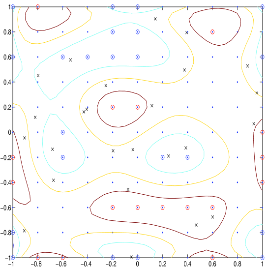
Figure 1: Point sets $X$ (25 crosses), $T$ (121 dots), and extremal points (39 circles around points of $T$), with contours of the approximation error. The extremal points do not form an $H$-set. Signs are indicated by blue or red circles.

Ignoring what the optimizer says, and aiming at a smaller $\mu$, one can go for all points with errors above $\mu=0.0760$, for instance. This yields only 23 points, see Figure 2, and these do not form an $H$-set either. One might argue that $N=23$ is too small for $n=25$ to make an $H$-set possible, but here and in other examples on regular points one has dependent homogeneous equations for the $H$-set condition (2), reducing the degrees of freedom.

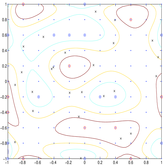
Figure 2: Point sets $X$ (25 crosses), $T$ (121 dots), and extremal points (23 circles around points of $T$), with contours of the approximation error. Two homogeneous conditions were dependent from the others, leading to a 23x23 situation. The extremal points do not form an $H$-set.

But one may take even more points, by allowing smaller $\mu$ and getting more degrees of freedom for the $H$-set, by admitting all points that have an absolute error of $\mu$ or more. It turns out that one has to go down to $\mu=0.0077$ to get an $H$ set of 112 points, see Figure 3. But for large $H$, the maximization of $1^{T}w$ shifts large weights to fewer components, and thus the set $H$ can be reduced by skipping the zero components. See Figure 4 showing the reduction from 112 to 27 points. Unfortunately, this reduction does not improve $\mu$ reasonably, because it does not select peak points. It works on coefficients, not on values.

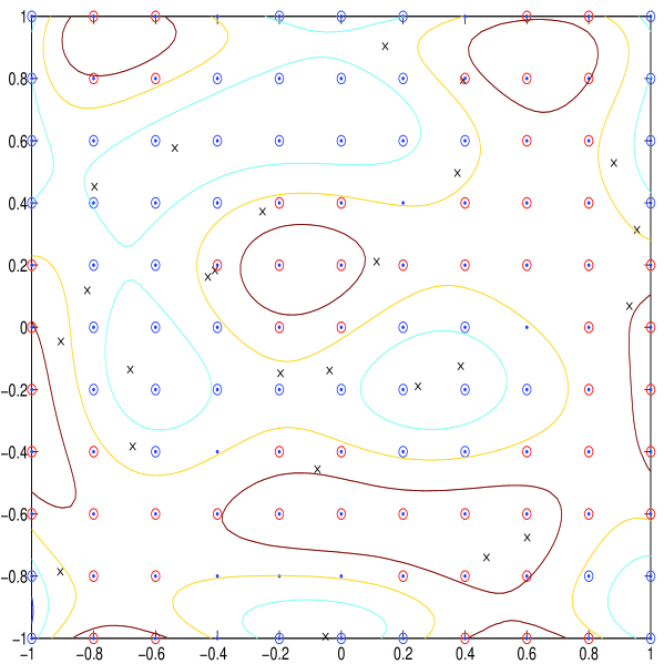
Figure 3: Point sets $X$ (25 crosses), $T$ (121 dots), and $H$-set (112 circles around points of $T$).

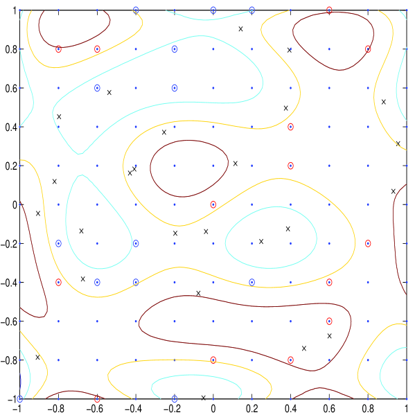
Figure 4: Point sets $X$ (25 crosses), $T$ (121 dots), and reduced $H$ set (27 circles around points of $T$)

6 Kernel-Based Divided Differences

We now consider the case $T=X\cup\{\xi\}$ with $\xi\notin X$ that works perfectly fine for univariate polynomial approximation, leading to alternation and divided differences. Generically, Chebyshev approximation by an $n$-dimensional space on a set of $n+1$ points should lead to “equioscillation”, i.e. the optimal error $\eta^{*}$ should be attained at all $n+1$ points, with different signs. But this cannot be expected in multivariate situations, and here we check the case of kernel-based trial spaces.

We go into the dual situation and apply existence and uniqueness of kernel-based interpolants to get the unique function $g_{\xi}\in V_{X\cup\{\xi\}}$ that vanishes on $X$ and is one at $\xi$. If we generally denote the Lagrangian with respect to a point $y\in Y$ and based on $Y$ as $u_{y}^{Y}$, the function $g_{\xi}$ is the Lagrangian $u_{\xi}^{X\cup\{\xi\}}$ and can be written as

$${\frac{1}{P_{X}^{2}(\xi)}}\left(K(x,\xi)-\sum_{i=1}^{n}u_{x_{i}}^{X}(x)K(x_{i},\xi)\right)$$

due to

$$K(\xi,\xi)-\sum_{i=1}^{n}u_{x_{i}}^{X}(\xi)K(x_{i},\xi)=P_{X}^{2}(\xi)$$

by definition of the Power Function $P_{X}$. The Lagrangians on $X$ have the form

$$u_{x_{i}}^{X}(x)=\sum_{j=1}^{n}\alpha^{X}_{ij}K(x,x_{j})$$

with the $\alpha^{X}_{i,j}$ being the elements of the (symmetric) inverse of the kernel matrix based on $X$. Then the $\ell_{1}$ norm of the coefficients of $g_{\xi}$ in the basis of $V_{X\cup\{\xi\}}$ is obtainable via

$$\begin{array}[]{rcl}K(x,\xi)-\sum_{i=1}^{n}u_{x_{i}}^{X}(x)K(x_{i},\xi)&=&K(x,\xi)-\sum_{i=1}^{n}\sum_{j=1}^{n}\alpha^{X}_{ij}K(x,x_{j})K(x_{i},\xi)\\ &=&K(x,\xi)-\sum_{j=1}^{n}K(x,x_{j})\sum_{i=1}^{n}\alpha^{X}_{ij}K(x_{i},\xi)\\ &=&K(x,\xi)-\sum_{j=1}^{n}K(x,x_{j})\sum_{i=1}^{n}\alpha^{X}_{ji}K(x_{i},\xi)\\ &=&K(x,\xi)-\sum_{j=1}^{n}K(x,x_{j})u_{x_{j}}^{X}(\xi)\\ \end{array}$$

as

$${\frac{1}{P_{X}^{2}(\xi)}}\left(1+\sum_{j=1}^{n}|u_{x_{j}}^{X}(\xi)|\right)=\displaystyle{\frac{1+L_{X}(\xi)}{P_{X}^{2}(\xi)}}$$

using the definition of the Lebesgue function $L_{X}$. The solution vector $w^{*}_{T}$ for the dual problem thus is unique and has coefficients

$$\begin{array}[]{rcl}\displaystyle{\frac{1}{1+L_{X}(\xi)}}&&\hbox{ at }\xi\\ \displaystyle{\frac{-u_{x_{i}}^{X}(\xi)}{1+L_{X}(\xi)}}&&\hbox{ at }x_{i}\in X,\end{array}$$

up to a fixed sign, because the Power Function cancels out. Using the standard interpolant $s_{X,f}$ to $f$ on $X$ in its Lagrange representation, and ignoring a possible sign of $w^{*}_{T}$, we find

$$f_{T}^{T}w^{*}_{T}=\displaystyle{\frac{f(\xi)-s_{X,f}(\xi)}{1+L_{X}(\xi)}},$$

and this is the analog of the divided difference in the context of discrete Chebyshev approximation on $n+1$ points. In fact, its absolute value

$$\begin{array}[]{rcl}|f_{T}^{T}w^{*}_{T}|&=&\displaystyle{\frac{|f(\xi)-s_{X,f}(\xi)|}{1+L_{X}(\xi)}}\\ &=&\eta^{*}(f,X\cup\{\xi\})\end{array}$$ (6)

determines the maximal error $\eta^{*}(f,X\cup\{\xi\})$ for the best discrete approximation $s^{*}_{X,\xi,f}$ to $f$ from the space $V_{X}$ on $X\cup\{\xi\}$, because there is no duality gap and $w_{T}^{*}$ can only change by its sign. The complementary slackness conditions finally produce an $H$-set consisting of $\xi$ and the points $x_{i}$ of $X$ for which $u_{x_{i}}(\xi)$ is nonzero. These must be extremal points, and the sign there is the sign of $u_{x_{i}}(\xi)$. Note that [8] has a similar notion of divided differences in context with Newton bases.

In the polynomial case, all Lagrangians must be nozero at additional points due to the Fundamental Theorem of Algebra, must change signs between zeros, and therefore one has alternation on all points of $X\cup\{\xi\}$. In the kernel case, the absolute errors in all $n+1$ points are equal as long as $\xi$ does not lie on a zero set of one of the Lagrangians $u_{x_{j}}^{X}$. This may be called the “nondegenerate” situation of full equioscillation, if degeneration counts the number of points where the error is not extremal. Generically, through each $x_{j}\in X$ there will be $n-1$ zero sets defined by the other Lagrangians. See Figure 5 for the case of the numerical example of Section 5 using 25 scattered points in $[-1,+1]^{2}$. If $\xi$ does not hit one of the curves, there will be no degeneration, and if $\xi$ moves over the zero curve of $u_{x_{j}}^{X}$, the sign of the error at $x_{j}$ will swap. In view of multiple intersections, the orders of degeneration may vary, but with probability one there is no degeneration, if $\xi$ is sampled uniformly over $[-1,+1]^{2}$.

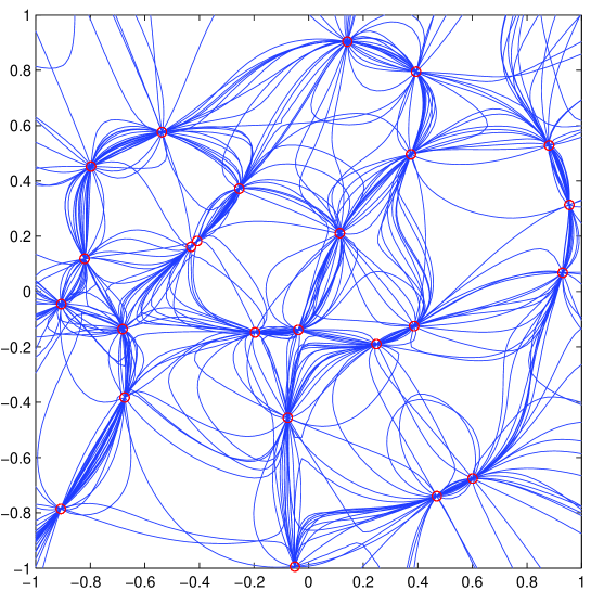
Figure 5: Zero sets of Lagrangians for the 25 points of $X$ (red circles) using the Gaussian at scale one.

Figure 6 shows the divided difference as a function of $\xi\in[-1,+1]^{2}$, while Figure 7 shows the zero set of the standard interpolation error. Note that the points of the zero set can be added to $X$ without changing the interpolant. This means that the usual error bounds in terms of fill distances

$$h(X,\Omega):=\sup_{y\in\Omega}\;\;\min_{x\in X}\|x-y\|_{2}$$

should be replaced by the $f$-dependent quantity

$$\sup_{y\in\Omega}\;\;\inf\{\|x-y\|_{2}\;:\;f(x)=s_{X,f}(x)\}\leq h(X,\Omega).$$

The $f$-greedy point selection strategy of [7] works similarly, but picks extrema of the current interpolation error $f-s_{X,f}$, not points of largest distance to the zero set. It could as well be changed to pick the point $\xi$ where the right-hand side of (6) is maximal. These variations are open for further research.

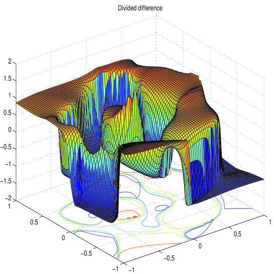
Figure 6: Divided difference as a function of $\xi$ for the 25 points of $X$ using the Gaussian at scale one and approximating the peaks function.

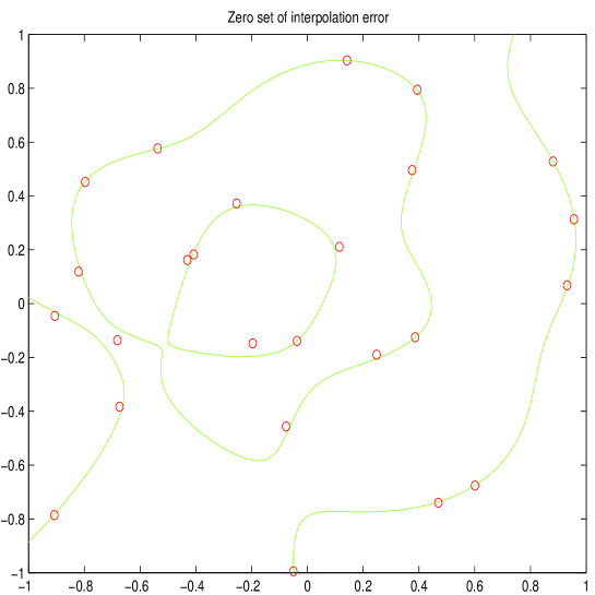
Figure 7: Zero set of the interpolation error on the 25 points of $X$ (red circles) using the Gaussian at scale one and interpolating the peaks function.

There is not much known about what happens for interpolation or approximation using unsymmetric kernel matrices with entries $K(t_{k},x_{j}),\;1\leq k\leq N,\;1\leq j\leq n$. The above case $N=n+1$ with $T=X\cup\{\xi\}$ is a first step.

References

- [1] M. Brannigan. H-sets in Linear Approximation. J. of Approx. Th., 20:153–161, 1977.
- [2] M. Brannigan. A geometric characterization of H-sets. J. of Approx. Th., 39:202–210, 1983.
- [3] M. D. Buhmann. Radial Basis Functions. Cambridge Monographs on Applied and Computational Mathematics. Cambridge University Press, 2004.
- [4] L. Collatz. Approximation von Funktionen bei einer und bei mehreren unabhängigen Veränderlichen. Angew. Math. und Mechanik (ZAMM), 36:198–211, 1956.
- [5] C. Dierieck. Some Remarks on H-Sets in Linear Approximation Theory. J. of Approx. Th., 21:188–204, 1977.
- [6] G. Fasshauer and M. McCourt. Kernel-based Approximation Methods using MATLAB, volume 19 of Interdisciplinary Mathematical Sciences. World Scientific, Singapore, 2015.
- [7] St. Müller. Komplexität und Stabilität von kernbasierten Rekonstruktionsmethoden. PhD thesis, University of Göttingen, 2009.
- [8] St. Müller and R. Schaback. A Newton basis for kernel spaces. Journal of Approximation Theory, 161:645–655, 2009. doi:10.1016/j.jat.2008.10.014.
- [9] G.D. Taylor. On minimal H-Sets. J. of Approx. Th., 5:113–117, 1972.
- [10] H. Wendland. Scattered Data Approximation. Cambridge University Press, 2005.
- [11] W. Wetterling. H-Mengen und Minimalbedingungen bei Approximationsproblemen. In R. Ansorge, K. Glashoff, and B. Werner, editors, Numerische Mathematik, Symposium anläßlich der Emeritierung von Lothar Collatz am Institut für Angewandte Mathematik, Universität Hamburg, vom 25.-26. Januar 1979, volume 49 of ISNM International Series of Numerical Mathematics, pages 195–204, 1979.