Shape Optimization for the Mitigation of Coastal Erosion via the Helmholtz Equation
Department of Mathematics
Universität Trier
Universitätsring 15, 54296 Trier
schlegel@uni-trier.de
&
Department of Mathematics
Universität Trier
Universitätsring 15, 54296 Trier
volker.schulz@uni-trier.de
Abstract
Coastal erosion describes the displacement of land caused by destructive sea waves, currents or tides. Major efforts have been made to mitigate these effects using groins, breakwaters and various other structures. We try to address this problem by applying shape optimization techniques on the obstacles. A first approach models the propagation of waves towards the coastline, using a 2D time-harmonic system based on the famous Helmholtz equation in the form of a scattering problem. The obstacle’s shape is optimized over an appropriate cost function to minimize the height of water waves along the shoreline, without relying on a finite-dimensional design space, but based on shape calculus.
Keywords Coastal Erosion Shape Optimization Helmholtz Equation
1 Introduction
Coastal erosion describes the displacement of land caused by destructive sea waves, currents or tides. Major efforts have been made to mitigate these effects using groins, breakwaters and various other structures. Among experimental set-ups to model the propagation of waves towards a shore and to find optimal wave-breaking obstacles, the focus has turned towards numerical simulations due to the continuously increasing computational performance. Essential contributions to the field of numerical coastal protection have been made for steady [1][2][3] and unsteady [4][5] descriptions of propagating waves. In this paper we select the Helmholtz Equation, that originates from the wave equation via separation of variables and assuming time independence. This paper builds up on the monographs [6][7][8] to perform free-form shape optimization. In addition we strongly orientate on [9][10][11] that use the Lagrangian approach for shape optimization, i.e. calculating state, adjoint and the deformation of the mesh via the volume form of the shape derivative assembled on the right-hand-side of the linear elasticity equation, as Riesz representative of the shape derivative. The application of shape-calculus-based shape optimization to prevent coastal erosion by optimizing the form of the Helmholtz scatterer builds an extension to [1], who relied on a fixed parametrization and to [3], who used a level set method for shape optimization. The paper is structured as follows: In Section 2 we formulate the PDE-constrained optimization problem. In Section 3 we will derive the necessary tools to solve this problem, by deriving the adjoint equation, the shape derivative in volume form and boundary form such as the topological derivative. The final part, Section 4, will then apply the results to firstly a simplified mesh and secondly to a more realistic mesh, picturing the Langue-de-Barbarie, a coastal section in the north of Dakar, Senegal that was severely affected by coastal erosion within the last decades.
2 Model Formulation
Suppose we are given an open domain , which is split into the disjoint sets such that , and . In this setting we assume the variable, interior and the fixed outer boundary to be at least Lipschitz. One simple example of such kind is visualized below in Figure 1.
We interpret as coastline, and as lateral sea, as open sea and as obstacle boundary. The PDE-constrained optimization problem on this domain is defined as [1]
| (1) | ||||||||
| s.t. | on | (2) | ||||||
| on | (3) | |||||||
| on | (4) | |||||||
| on | (5) | |||||||
Remark.
The PDE constrained optimization problem is mainly taken from [1], however we will tackle the problem by not relying on a finite design space but on shape calculus.
2.1 Wave Description
On the illustrative domain we intend to model water waves by complex solution field to the stationary elliptic Helmholtz equation, i.e.
| (6) |
The complexity is introduced for a total field consisting of , since the incoming wave is defined as , where is a constant wavenumber, the amplitude or maximal surface elevation and the wave direction with for .
In the course of this chapter we will also deal with a second problem, placing a transmissive obstacle in for porosity coefficient . For this we firstly modify the problem such that we are solving for two distinct wave fields on and (cf. to [12]), i.e.
| (7) | ||||||
| (8) |
for transmission boundaries
| (9) | |||||
for normal vector . The two wave fields can be rewritten by the usage of a discontinuous transmission coefficient
| (10) |
with interface boundary conditions in the sense of (9) as
| (11) | ||||
Remark.
The latter approach requires calculations on , such that we can write integrals as
| (12) |
Remark.
The obstacles can in the transmissive case be interpreted as permeable with regards to propagating waves, e.g. in [2] geotextile tubes are proposed.
Remark.
Remark.
Choosing let us solve the classical Helmholtz equation on the whole domain.
2.2 Periodic Boundary Condition
Periodic boundary conditions are used as
| (13) |
Remark.
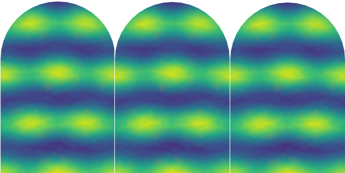
These conditions allow to significantly reduce the computational domain size, e.g. instead of modelling the whole coastline, it allows the field calculation for a reduced domain assuming periodic reproducibility along the shore (cf. exemplifying to Figure 2).
2.3 Sommerfeld Radiation Condition
The model with is equipped with open or non-reflecting boundary at sea level in form of the Sommerfeld Radiation Condition [13]. It ensures the uniqueness of the solution by demanding that scattered waves are not reflected at an infinite boundary by requiring
| (14) | ||||
| (15) |
Since we are restricted to a finite domain, we adjust the condition using the first order approximation [1] on
| (16) |
where due to the half circled boundary for radial distance .
2.4 Partially Absorbing Boundary Condition
We assume partial reflection of the waves at the coast and at the obstacle, by partial absorbing boundary condition (3) on and , i.e.
| (17) |
where represents the complex transmission coefficient as introduced in [16].
Remark.
The general solution was derived by Berkhoff [16] for as
| (18) | |||
with reflection coefficient , reflection phase angle and the incident wave direction .
Remark.
The choice of is a priori a rocky question as it needs to incorporate the angle of the incoming such as already already scattered waves. Since the preceding formulation is based on the assumption that the transmission coefficient is known for all parts of the boundary, we follow [17] for simplification and set and , which leads for (18) to:
| (19) | ||||
Remark.
In [1] and [3] the simple case for is considered such that (3) reduces to which is commonly referred to as sound-hard scattering [18] implying
| (20) |
This assumption simplifies not only the calculation for the field but also for the shape derivative as we will see in Section 3. However, this may lead to undesired reflections at respective boundaries.
2.5 Objective Function
An obstacle is considered to be optimal, if the squared difference of wave and target height is minimized and the distribution is as uniform as possible along the shore. Hence, we define the objective
-
1.
for single directions and frequencies as:
(21) for target height such as variance weight and mean elevation .
-
2.
for multiple directions with different weights each for different wave numbers as:
(22)
In either case to ensure that the obstacle is not becoming arbitrarily large we add a volume penalty controlled by , i.e.
| (23) |
and a perimeter regularization, controlled by the parameter as
| (24) |
3 Adjoint-Based Shape & Topology Optimization
In this section we will first introduce the necessary tools for adjoint-based shape optimization, before we apply techniques to the PDE-constrained problem from the previous section.
3.1 Notations and Definitions
The idea of shape optimization is to deform an object ideally to minimize some target functional. Hence, to find a suitable matter of deforming we are interested in some shape analogy of a classical derivative. Here we use a methodology that is commonly used in shape optimization and extensively elaborated in various works [6][7][8].
In this section we fix notations and definitions following [10][11] and amend whenever it appears necessary.
We start by introducing a family of mappings for that are used to map each current position to another by , where we choose the vector field as the direction for the so called perturbation of identity
| (26) |
According to this methodology, we can map the whole domain to another such that
| (27) |
Minimization of a generic functional dependent on the domain often requires the derivatives. Hence, we define the Eulerian Derivative as
| (28) |
Commonly, this expression is called shape derivative of at in direction and in this sense shape differentiable at if for all directions the Eulerian derivative exists and the mapping is linear and continuous. In addition, we define the material derivative of some scalar function at with respect to the deformation as
| (29) |
and the corresponding shape derivative for a scalar . In the following, we will use the abbreviation to mark the material derivative of . In Section 3 we will need to have the following calculation rules on board [20]
| (30) | ||||
| (31) | ||||
| (32) |
The basic idea in the proof of the shape derivative in the next section will be to pull back each integral defined on the on the transformed field back to the original configuration. We therefore need to state the following rule for differentiating domain integrals [20].
| (33) |
3.2 Adjoint-Based Shape & Topology Optimization
We reformulate the constrained optimization problem (1)-(5) with the help of the Lagrangian
| (34) |
where is the objective (21), is the bilinear form obtained from boundary value problem (2)-(5) and are multipliers.
| (35) | ||||
and is the bilinear form defined by
| (36) |
Remark.
The transmissive case leads us to weak forms as
| (37) | ||||
and is the bilinear form defined by
| (38) |
where denotes the usage of jumps in the associated integrals.
Remark.
To continue with adjoint calculations we are required to integrate twice by parts on the derivative-containing terms such that we obtain exemplifying obtain for non-transmissive obstacle
| (39) | ||||
Remark.
Instead of multipliers it is also possible to derive adjoint and shape derivative based on an immediate insertion of boundary conditions.
Remark.
We can regard the Lagrangian (34) w.r.t. in the same manner. In the following we restrict to for readability.
We obtain the state equation from differentiating the Lagrangian for and the adjoint equation from differentiating w.r.t. . As in [9], the theorem of Correa and Seger [21] is applied on the right hand side of (40) so that the following equality holds
| (40) |
The adjoint is formulated in the following theorem:
Theorem 1.
(Adjoint) Assume that the elliptic PDE problem (2)-(5) is -regular and as in (19), so that its solution is at least in . Then the adjoint in strong form (without perimeter regularization and variance penalty) is given by
| on | (41) | |||||
| on | ||||||
| on | ||||||
| on | ||||||
| on |
Proof.
Any directional derivative of w.r.t. must be zero at the solution , hence
| (42) | ||||
From this we get the adjoint in strong form for the domain by taking the variation as , we obtain
| (43) |
In addition leads to
| (44) |
From this we know that on and , such as on and on and . With this, leads to
| (45) | ||||
Which provides us with boundary conditions for normal as claimed, due to the complex symmetry of the complex inner product. ∎
Having computed both and we can go over and compute the shape derivative (28).
Remark.
Shape derivatives can for a sufficiently smooth domain be described via boundary formulations using Hadamard’s structure theorem [7]. The integral over is then replaced by an integral over that acts on the associated normal vector. In this paper we calculate the deformation field based on the domain formulation and use the boundary formulation for the topological derivative.
Theorem 2.
(Shape Derivative Volume Form) Assume that the elliptic PDE problem (2)-(5) is -regular, so that its solution is at least in . Moreover, assume that the adjoint equation (41) admits a solution . Then the shape derivative of the objective (without perimeter regularization for full-reflecting boundaries) at in the direction is given by
| (46) | ||||
Proof.
The basic idea is to pull all expressions back to the original configuration [19]. For readability we analyse each term by its own. We note that all terms, including the objective, solely dependent on boundaries other than vanish, since these are defined to be invariant under perturbations of the domain. We start by terms of leading order, where we first use (33) e.g.
| (47) |
Then the first integral is rewritten using (32)
| (48) | ||||
For the second integral we obtain again using (33)
| (49) |
Similar to before the first integral is rewritten using (30), such that we get
| (50) |
If we finally rearrange the terms with and , let them act as test functions, apply the saddle point conditions, which means that the state equation (41) and adjoint equation (41) are fulfilled, the terms consisting and cancel. By adding all terms above up and using the definition of the inner product (25), the shape derivative is established. ∎
Remark.
In case of partial reflection the boundary terms are obtained by observing
| (51) |
with the convention
| (52) |
and applying saddle point conditions.
Having obtained the Helmholtz shape derivative in volume form we can now deduce the shape derivate in surface form.
Theorem 3.
(Shape Derivative Boundary Form) Under the assumptions of Theorem 2 the shape derivative of the objective (without perimeter regularization for full-reflecting boundaries) at in the direction is given by
| (53) |
Proof.
Remark.
Following [22] we are now in the position to derive the topological derivative as described in the following theorem.
Theorem 4.
(Topological Derivative) Under the assumptions of Theorem 2 the topological derivative of the objective (without perimeter regularization for full-reflecting boundaries) is given as
| (54) |
Proof.
Finally for completeness we require the shape derivative of the volume penalty and the perimeter regularization as [7]
| (56) | ||||
| (57) |
4 Numerical Results
In this section we firstly describe the numerical algorithm to solve the PDE-constrained optimization problem and present applications to a simplistic domain for transmissive and non-transmissive obstacle such as a domain representing the Langue-de-Barbarie a coastal section in the north of Senegal.
4.1 Implementation Details
We are relying on the classical structure of adjoint-based shape optimization algorithms gradient-descent algorithms. However, we motivate the location and shape of the initial obstacle by the usage of the topological derivative (54), that means we are exploiting the obtained scalar field to initialize an obstacle with the help of a filter which is based on the density-based spatial clustering algorithm (DBSCAN) [25]. The obstacle is then deformed in a second step by the the usage of shape optimization. The procedure is shortly sketched in Figure 3.
To compute the solution to the boundary value problem (2)-(5), the adjoint problem (41) and to finally deform the domain we are relying on the finite element solver FEniCS [26]. High accuracy for the elliptic, constraining PDE is achieved using a Continuous Galerkin (CG) method of order to discretize in space. The mentioned deformation or update of the finite element mesh in each iteration is done via the solution of the linear elasticity equation, which stems from the usage of the Steklov-Poincaré metric [10]
| (58) | |||||
where and are called strain and stress tensor and and are called Lame parameters. In our calculations we have chose and as the solution of the following Poisson Problem
| in | (59) | |||||
| on | ||||||
| on |
The source term in (58) consists of a volume and surface part, i.e. . Here the volumetric share comes from our Helmholtz shape derivative and the shape derivative volume penalty , where we only assemble for test vector fields whose support intersects with the interface and is set to zero for all other basis vector fields. The surface part comes from the shape derivative parameter regularization .
Remark.
In order to guarantee the attainment of useful shapes, which minimize the objective, a backtracking line search is used, which limits the step size in case the shape space is left [27] i.e. having intersecting line segments or the objective is non-decreasing.
Remark.
Solutions to state, adjoint and shape derivative, require the manual calculation of the real part by splitting all occurring trial and test functions in real and imaginary part.
4.2 Ex.1: The Simplistic Mesh
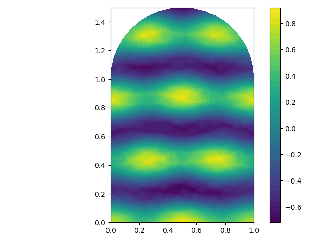
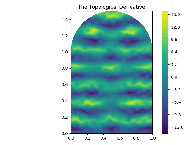
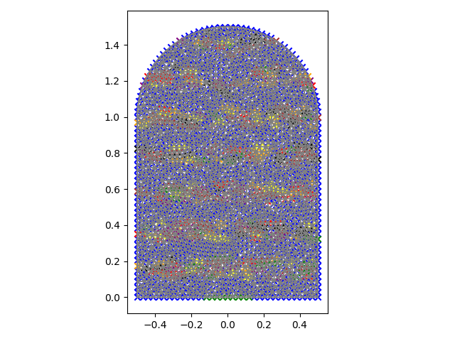
In the first example, we will look at the model problem, that was described in Section 2. We interpret and as the reflective coastline and obstacle, and as the lateral, such as as the open sea boundary. As it is described before in Section 4, the topological derivative can be used in line with a filter to determine the location of an initial obstacle. Exemplifying, we show in Figure 4 an initial field on the simplistic mesh for which the topological derivative is calculated. A filter in form of a DBSCAN-algorithm is then used in Figure 5 to initialize an obstacle. Here results are shown for a minimum number of points in a cluster and threshold , where colours apart from blue build useful clusters.
We have used this information to generate the meshes in Figure 6 with the the mesh generator GMSH [28]. We have discretized finer around the obstacle to ensure a high resolution for the shape optimization routine. A reducing effect along the shore of the created meshes for single and multi-wave case can already be observed for the pure placement of the obstacles in Figure 7. The forthcoming analysis is based on wave description (2), we firstly model a single wave perpendicular to the obstacle’s lower boundary by choosing and a suitable wave number e.g. in the first two figures of Figures 7 and 8. In the multi wave case (22) we model the sum of waves with for weights such as frequencies with , which can be taken from the third figures in Figures 7, 8 and can be interpreted as strong waves from north-west. In all the test cases we model full reflection, i.e. . In the objective we enforce regularization of the perimeter by a weight of . The solution to the state and adjoint equation is of linear nature, hence we use the FEniCS solver for linear partial differential equations. Having solved state and adjoint equations the mesh deformation is performed as described before, where we specify and in (59). The step size is at and shrinks whenever criteria for line searches are not met. We can extract results of shape optimization from Figure 8, where we due to Figure 9 have obtained a significant decrease in the objective values.
We now turn towards the transmissive obstacle case, i.e. (7)-(9) is used. Wave-settings equal to the mono-wave from before but working with a discontinuous porosity coefficient for and , that is pictured in Figure 10. We remark that for an appropriate evaluation of the weak form (2) the discontinuity must be inline with the positioning of the mesh nodes. We then once more target to track a specified height of field (cf. to Figure 10, 1., left). The optimized form, which can be seen in Figure 11, is especially notable. It forms two lines of vertically shifted stretched obstacles, which is due to the initial placement of the obstacle, participating on two increased fronts in the scalar field of the topological derivative (cf. to Figure 4). The shape is then minimized in areas of low values for the mentioned scalar field. The final shape was reached after iterations, where the norm of the gradient reached the convergence threshold. The convergence of the objective function can be taken from Figure 11.
4.3 Ex.2: Langue-de-Barbarie
A more realistic computation is performed in the second example. Here we look at the Langue-de-Barbarie a coastal section in the north of Dakar, Senegal. In 1990 it consisted of a long offshore island, which eroded in three parts within two decades. Waves now travel unhindered to the mainlands, which causes severe damage and destroyed large habitats. Adjusting our model to this specific coastal section starts on mesh level. Shorelines are taken from the free GSHHG databank222https://www.ngdc.noaa.gov/mgg/shorelines/ following [29]. We build an interface from a geographical information system (QGIS3) for processing the data to the Computer Aided Design software GMSH for the mesh generation. Similar to the preceding example, we interpret as coastline for islands and mainlands such as the open sea boundary. We have inserted a smaller island, which shape is to be optimized in front of the second and third with boundary denoted as (cf. to Figure 13,14). The waves propagation is modelled mono-directionally to the shores with and . The initial mesh can be extracted from Figure 12.
Figures 13 and 14 picture fields to the optimized meshes for and using (19) and an initial step size after and steps of optimization.
One can observe a similar behaviour as in Subsection 4.2, where the obstacle is stretched to protect an as large as possible area. The computation stopped after obtaining intersecting line segments at the obstacle’s centre in Figure 13 and reaching the convergence threshold for the norm of the gradient in Figure 14. However, in Figures 15 and 16 we can still note a significant decrease in the target functional for both cases, taking into account that the area of the scatterer is comparably low to the area of the shorelines.
Remark.
From a practical, durability standpoint thin obstacles as in Figures 8 and 13, which also lead to breakdown of the optimization algorithm, due to intersecting line segments, are not ideal. To circumvent this problem we have used a thinness penalty (cf. to [30]) in works dealing with Shallow Water Equations [31][32], but this should not be treated here.
5 Conclusion
We have derived the stationary continuous adjoint and shape derivative in volume form for the Helmholtz equation with suitable boundary conditions. The results were tested on a 2-dimensional simplistic domain and a more comprehensive one picturing the Langue-de-Barbarie coastal section. The optimized shape strongly orients itself to wave directions and to the respective coastal section that is to be protected. The results can be easily adjusted for arbitrary meshes, objective functions and different wave such as boundary properties.
Acknowledgement
This work has been supported by the Deutsche Forschungsgemeinschaft within the Priority program SPP 1962 "Non-smooth and Complementarity-based Distributed Parameter Systems: Simulation and Hierarchical Optimization". The authors would like to thank Diaraf Seck (Université Cheikh Anta Diop, Dakar, Senegal) and Mame Gor Ngom (Université Cheikh Anta Diop, Dakar, Senegal) for helpful and interesting discussions within the project Shape Optimization Mitigating Coastal Erosion (SOMICE).
References
- [1] Pascal Azerad, Benjamin Ivorra, Bijan Mohammadi, and Frédéric Bouchette. Optimal Shape Design of Coastal Structures Minimizing Coastal Erosion. 01 2005.
- [2] Damien Isebe, Pascal Azerad, Frédéric Bouchette, Benjamin Ivorra, and Bijan Mohammadi. Shape optimization of geotextile tubes for sandy beach protection. International Journal for Numerical Methods in Engineering, 74:1262 – 1277, 05 2008.
- [3] Moritz Keuthen and D. Kraft. Shape optimization of a breakwater. Inverse Problems in Science and Engineering, 24, 09 2015.
- [4] Bijan Mohammadi and Afaf Bouharguane. Optimal dynamics of soft shapes in shallow waters. Computers & Fluids, 40:291–298, 01 2011.
- [5] Afaf Bouharguane and Bijan Mohammadi. Minimization principles for the evolution of a soft sea bed interacting with a shallow. International Journal of Computational Fluid Dynamics, 26:163–172, 03 2012.
- [6] Kyung K. Choi. Shape design sensitivity analysis and optimal design of structural systems. In Carlos A. Mota Soares, editor, Computer Aided Optimal Design: Structural and Mechanical Systems, pages 439–492, Berlin, Heidelberg, 1987. Springer Berlin Heidelberg.
- [7] J. Sokołowski and J.P. Zolésio. Introduction to shape optimization: shape sensitivity analysis. Springer series in computational mathematics. Springer-Verlag, 1992.
- [8] M. C. Delfour and J. P. Zolésio. Shapes and Geometries. Society for Industrial and Applied Mathematics, second edition, 2011.
- [9] Volker Schulz, Martin Siebenborn, and Kathrin Welker. Structured inverse modeling in parabolic diffusion processess. SIAM Journal on Control and Optimization, 53, 09 2014.
- [10] Volker H. Schulz, Martin. Siebenborn, and Kathrin. Welker. Efficient pde constrained shape optimization based on steklov–poincaré-type metrics. SIAM Journal on Optimization, 26(4):2800–2819, 2016.
- [11] Volker Schulz and Martin Siebenborn. Computational comparison of surface metrics for pde constrained shape optimization, 2016.
- [12] G. Yan; P. Y.H. Pang. The uniqueness of the inverse obstacle scattering problem with transmission boundary conditions. Pergamon Computers Math. Applic. Vol. 36, 1997.
- [13] Steven H Schot. Eighty years of sommerfeld’s radiation condition. Historia Mathematica, 19(4):385 – 401, 1992.
- [14] Joseph J. Shirron and Ivo Babuška. A comparison of approximate boundary conditions and infinite element methods for exterior helmholtz problems. Computer Methods in Applied Mechanics and Engineering, 164(1):121–139, 1998. Exterior Problems of Wave Propagation.
- [15] Eliane Becache, Anne-Sophie Bonnet-Ben Dhia, and Guillaume Legendre. Perfectly matched layers for the convected helmholtz equation. SIAM J. Numerical Analysis, 42:409–433, 01 2004.
- [16] J. C. W. Berkhoff. Mathematical Models for Simple Harmonic Linear Water Waves: Wave Diffraction and Refraction. PhD thesis, Delft Hydraulics Lab. (Netherlands)., 4 1976.
- [17] Michael Isaacson and Shiqin Qu. Waves in a harbour with partially reflecting boundaries. Coastal Engineering, 14(3):193 – 214, 1990.
- [18] David Colton and Rainer Kress. Inverse acoustic and electromagnetic scattering theory. 1992.
- [19] Gonzalo Feijóo, Assad Oberai, and Peter Pinsky. An application of shape optimization in the solution of inverse acoustic scattering problems. Inverse Problems, 20(1):199–228, 12 2003.
- [20] Martin Berggren. A Unified Discrete–Continuous Sensitivity Analysis Method for Shape Optimization, volume 15, pages 25–39. 08 2010.
- [21] Rafael Correa and Alberto Seeger. Directional derivative of a minmax function. Nonlinear Analysis-theory Methods & Applications, 9:13–22, 01 1985.
- [22] Gonzalo Feijoo. A new method in inverse scattering based on the topological derivative. Inverse Problems, 20:1819, 09 2004.
- [23] Raúl Feijóo, A.A. Novotny, Edgardo Taroco, and Claudio Padra. The topological derivative for the poisson problem. Mathematical Models and Methods in Applied Sciences, 13:1825–1844, 12 2003.
- [24] A.A. Novotny and Jan Sokolowski. Topological Derivatives in Shape Optimization. Interaction of Mechanics and Mathematics Series. 01 2013.
- [25] Martin Ester, Hans-Peter Kriegel, Jörg Sander, and Xiaowei Xu. A density-based algorithm for discovering clusters in large spatial databases with noise. pages 226–231. AAAI Press, 1996.
- [26] Martin S. Alnæs, Jan Blechta, Johan Hake, August Johansson, Benjamin Kehlet, Anders Logg, Chris Richardson, Johannes Ring, Marie E. Rognes, and Garth N. Wells. The fenics project version 1.5. Archive of Numerical Software, 3(100), 2015.
- [27] Kathrin Welker. Efficient PDE Constrained Shape Optimization in Shape Spaces. doctoralthesis, Universität Trier, 2017.
- [28] Christophe Geuzaine and Jean-François Remacle. Gmsh: A 3-d finite element mesh generator with built-in pre- and post-processing facilities. International Journal for Numerical Methods in Engineering, 79:1309 – 1331, 09 2009.
- [29] Alexandros Avdis, Christian Jacobs, Simon Mouradian, Jon Hill, and Matthew Piggott. Meshing ocean domains for coastal engineering applications. In VII European Congress on Computational Methods in Applied Sciences and Engineering, 06 2016.
- [30] Grégoire Allaire, François Jouve, and Georgios Michailidis. Thickness control in structural optimization via a level set method. Structural and Multidisciplinary Optimization, 53, 06 2016.
- [31] Luka Schlegel and Volker Schulz. Shape optimization for the mitigation of coastal erosion via shallow water equations, 2021.
- [32] Luka Schlegel and Volker Schulz. Shape optimization for the mitigation of coastal erosion via porous shallow water equations, 2021.