Linear spectral statistics of sequential sample covariance matrices

Abstract

Let $\mathbf{x}_{1},\ldots,\mathbf{x}_{n}$ denote independent $p$-dimensional vectors with independent complex or real valued entries such that $\mathbb{E}[\mathbf{x}_{i}]=\mathbf{0}$, ${\rm Var}(\mathbf{x}_{i})=\mathbf{I}_{p}$, $i=1,\ldots,n$, let $\mathbf{T}_{n}$ be a $p\times p$ Hermitian nonnegative definite matrix and $f$ be a given function. We prove that an approriately standardized version of the stochastic process $\big{(}{\operatorname{tr}}(f(\mathbf{B}_{n,t}))\big{)}_{t\in[t_{0},1]}$ corresponding to a linear spectral statistic of the sequential empirical covariance estimator

$$\big{(}\mathbf{B}_{n,t})_{t\in[t_{0},1]}=\Big{(}\frac{1}{n}\sum_{i=1}^{\lfloor nt\rfloor}\mathbf{T}^{1/2}_{n}\mathbf{x}_{i}\mathbf{x}_{i}^{\star}\mathbf{T}^{1/2}_{n}\Big{)}_{t\in[t_{0},1]}$$

converges weakly to a non-standard Gaussian process for $n,p\to\infty$. As an application we use these results to develop a novel approach for monitoring the sphericity assumption in a high-dimensional framework, even if the dimension of the underlying data is larger than the sample size.

Keywords: linear spectral statistic, sequential sample covariance matrix, sequential process, sphericity test, Stieltjes transform, monitoring spherictiy.

AMS subject classification: Primary 15A18, 60F17; Secondary 62H15

1 Introduction

Estimation and testing of a high-dimensional covariance matrix is a fundamental problem of statistical inference with numerous applications in biostatistics, wireless communications and finance (see, e.g., Fan and Li, (2006), Johnstone, (2006) and the references therein). Linear spectral statistics are frequently used to construct tests for various hypotheses. For example, Mauchly, (1940) proposes a likelihood ratio test for the hypothesis of sphericity (of a normal distribution), which has been extended by Gupta and Xu, (2006) to the non-normal case and by Bai et al., (2009) and Wang and Yao, (2013) to the high-dimensional case, where the dimension $p$ is of the same order as the sample size $n$, that is $p/n\to y\in(0,1)$ as $p,n\to\infty$ (see also Theorem 9.12 in the monograph of Yao et al., (2015) for a further extension). Alternative tests based on distances between the sample covariance matrix and a multiple of the identity matrix have been considered in Ledoit and Wolf, (2002) and Chen et al., (2010) among others. Fisher et al., (2010) suggest a generalization of John’s test for sphericity, which is based on a ratio of arithmetic means of the eigenvalues of different powers of the sample covariance matrix. Among other testing problems such as sphericity, Jiang and Yang, (2013) consider some classical $q$-sample testing problems under normality in a high-dimensional setting, which are further generalized in Dette and Dörnemann, (2020) for an increasing number $q$ of groups. Other authors concentrate on linear spectral statistics of $F$-matrices (see, for example, Zheng, , 2012; Zheng et al., , 2017; Bodnar et al., , 2019), auto-cross covariance (Jin et al., , 2014), large-dimensional matrices with bivariate dependence measures as entries (Bao et al., 2015a, ; Li et al., , 2019) or information-plus-noise matrices (Banna et al., , 2020).

Because of its importance in statistics numerous authors have investigated the asymptotic properties of linear spectral statistics from a more general perspective. An early reference is Jonsson, (1982) and in their pioneering paper, Bai and Silverstein, (2004) proved a central limit theorem for linear spectral statistics of the form

$$\sum_{i=1}^{p}f(\lambda_{i}(\mathbf{B}_{n}))$$

of the sample covariance matrices $\mathbf{B}_{n}=\frac{1}{n}\sum_{i=1}^{n}\mathbf{T}^{1/2}_{n}\mathbf{x}_{i}\mathbf{x}_{i}^{\star}\mathbf{T}^{1/2}_{n}$ under rather general conditions, where $\mathbf{x}_{1},\ldots,\mathbf{x}_{n}$ are independent $p$-dimensional random vectors with independent real or complex valued (centered) entries $x_{ij}$, $\mathbf{T}_{n}$ is a $p\times p$ (non-random) Hermitian nonnegative definite matrix and $\lambda_{1}(\mathbf{B}_{n})\leq\ldots\leq\lambda_{p}(\mathbf{B}_{n})$ are the ordered eigenvalues of the matrix $\mathbf{B}_{n}$. Several authors have followed this line of research and tried to relax the assumptions for such statements (see Pan and Zhou, , 2008; Lytova and Pastur, , 2009; Pan, , 2014; Zheng et al., , 2015; Najim and Yao, , 2016, among others).

In this paper we will take a different point of view on linear spectral statistics and study these objects from a sequential perspetive. More precisely, we consider a sequential version of the empirical covariance estimator

$$\mathbf{B}_{n,t}=\frac{1}{n}\sum_{i=1}^{\lfloor nt\rfloor}\mathbf{T}^{1/2}_{n}\mathbf{x}_{i}\mathbf{x}_{i}^{\star}\mathbf{T}^{1/2}_{n}~{},~{}~{}0\leq t\leq 1,$$ (1.1)

and investigate the probabilistic properties of the stochastic process corresponding to linear spectral statistics of $\mathbf{B}_{n,t}$, that is

$$S_{t}=\frac{1}{p}\sum_{i=1}^{p}f(\lambda_{i}(\mathbf{B}_{n,t}))~{},~{}~{}0\leq t\leq 1,$$ (1.2)

where $\lambda_{1}(\mathbf{B}_{n,t})\leq\ldots\leq\lambda_{p}(\mathbf{B}_{n,t})$ are the ordered eigenvalues of the matrix $\mathbf{B}_{n,t}$. In particular, we prove that for any $0<t_{0}<1$, an appropriately normalized and centered version of the process $(S_{t})_{t\in[t_{0},1]}$ converges weakly to non-standard Gaussian process.

Our interest in these processes is partially motivated by the fact that the sequential covariance estimator plays a central role in the construction of methodology for the detection of structural breaks in the covariance structure (see Aue et al., , 2009; Dette and Gösmann, , 2020, among others). In this field various functionals of the process $(\mathbf{B}_{n,t})_{~{}0\leq t\leq 1}$ have been studied in the case of fixed dimension, and we expect that results on the weak convergence of the process $(S_{t})_{t\in[t_{0},1]}$ will be useful in the context of change-point analysis for high-dimensional covariance covariance matrices. In fact, we use the probabilistic results presented in this paper to develop a procedure for monitoring deviations from sphericity, see Section 3 for more details.

Surprisingly, sequential processes of the form (1.2) have not found much attention in the literature. To our best knowledge we are only aware of the work of D’Aristotile, (2000) and Nagel, (2020), who considered sequential aspects of large dimensional random matrices from a different point of view. More precisely, D’Aristotile, (2000) studied a sequential process generated from the first $\lfloor nt\rfloor$ diagonal elements of a random matrix chosen according to the Haar measure on the unitary group of $n\times n$ matrices and showed that this process converges weakly to a standard complex-valued Brownian motion (see also D’Aristotile et al., , 2003, for similar results). Recently, Nagel, (2020) proved a functional central limit theorem for the sum of the first $\lfloor nt\rfloor$ diagonal elements of an $n\times n$ matrix $f(Z)$, where $Z$ has an orthogonal or unitarily invariant distribution such that ${\rm tr}\big{(}f(Z)\big{)}$ satisfies a CLT. Compared to these contributions the results of the present paper are conceptually different, because - in contrast to the cited references - the parameter $t$ used in the definition of the process (1.1) also appears in the eigenvalues $\lambda_{i}(\mathbf{B}_{n,t})$. This “non-linearity” results in a substantially more complicated structure of the problem. In particular, the limiting processes of $(S_{t})_{t\in[t_{0},1]}$ are non-standard Gaussian processes (except in the case $f(x)=x$), and the proofs of our results (in particular the proof of tightness) require an extended machinery, which has so far not been considered in the literature on linear spectral statistics. As a consequence we provide a substantial generalization of the classical CLT for linear spectral statistics (see, for example, Bai and Silverstein, , 2010), which is obtained from the process convergence of $(S_{t})_{t\in[t_{0},1]}$ (appropriately standardized) via continuous mapping.

2 A sequential look at linear spectral statistics

Let $\mathbf{x}_{1},\ldots,\mathbf{x}_{n}$ be independent $p$-dimensional random vectors with real or complex entries and covariance matrix given by the identity matrix $\mathbf{I}=\mathbf{I}_{p}\in\mathbb{R}^{p\times p}$ . We use the notation $\mathbf{x}_{j}=(x_{1j},\ldots,x_{pj})^{\top}$ for the components of $\mathbf{x}_{j}$ and assume that $\mathbb{E}[x_{ij}]=0$ and $\mathbb{E}[x_{ij}^{2}]=1$. When considering asymptotics, the dimension $p=p_{n}$ of the data is allowed to increase with the sample size $n\to\infty$ at same order, that is, $p/n\to y\in(0,\infty)$ as $n\to\infty$. Recall the notation of the sequential covariance estimator $\mathbf{B}_{n,t}$ in (1.1) and consider the corresponding linear spectral statistic (as a function of $t$)

$$S_{t}=\frac{1}{p}\operatorname{tr}\big{(}f(\mathbf{B}_{n,t})\big{)}=\frac{1}{p}\sum\limits_{j=1}^{p}f\left(\lambda_{i}(\mathbf{B}_{n,t})\right),~{}t\in[0,1],$$

where $f$ is an appropriate function defined on a subset of the complex plane. For a given $t_{0}\in(0,1]$, we are interested in the asymptotic properties of the process $(S_{t})_{t\in[t_{0},1]}$ and will prove a weak convergence result for an appropriately standardized version of this process in the space $\ell^{\infty}([t_{0},1])$ of bounded functions defined on the interval $[t_{0},1]$. Note that the random variable $S_{1}$ has been studied intensively in the literature (see the discussion in Section 1).

For the statement of our main result we require some notation. Let

$$F^{\mathbf{A}}=\frac{1}{p}\sum\limits_{j=1}^{p}\delta_{\lambda_{j}(\mathbf{A})},$$

be the empirical spectral distribution of a $p\times p$ Hermitian matrix $\mathbf{A}$, where $\lambda_{1}(\mathbf{A}),\ldots,\lambda_{p}(\mathbf{A})$ are the eigenvalues of $\mathbf{A}$ (often the dependence on $\mathbf{A}$ is omitted in the notation, because it is clear from the context) and $\delta_{a}$ denotes the Dirac measure at a point $a\in\mathbb{R}$. A useful tool in random matrix theory is the Stieltjes transform

$$s_{F}(z)=\int\frac{1}{\lambda-z}dF(\lambda)$$

of a distribution function $F$ on the real line, which is here defined for $z\in\mathbb{C}^{+}=\{z\in\mathbb{C}:\operatorname{Im}(z)>0\}$. If $F=F^{\mathbf{A}}$ is an empirical spectral distribution, then its Stieltjes transform has the form

$$s_{F^{\mathbf{A}}}(z)=\frac{1}{p}\operatorname{tr}\left\{\left(\mathbf{A}-z\mathbf{I}\right)^{-1}\right\},z\in\mathbb{C}^{+}.$$

Standard results on linear spectral statistics (see, for example the monograph of Bai and Silverstein, , 2010) show that (for fixed $t>0$) under certain conditions, with probability $1$, the empirical spectral distribution $F^{(n/\lfloor nt\rfloor)\mathbf{B}_{n,t}}$ of the (scaled) matrix $(n/\lfloor nt\rfloor)\mathbf{B}_{n,t}$ converges weakly. The limit, say $F^{y_{t},H}$, is the so-called generalized Marčenko-Pastur distribution defined by its Stieltjes transform $s_{t}=s_{F^{y_{t},H}}$, which is the unique solution of the equation

$$s_{t}(z)=\int\frac{1}{\lambda(1-y_{t}-y_{t}zs_{t}(z))-z}dH(\lambda)$$ (2.1)

on the set $\{s_{t}\in\mathbb{C}^{+}:\frac{1-y_{t}}{z}+y_{t}s_{t}\in\mathbb{C}^{+}\}$. Here, $H$ denotes the limiting spectral distribution $H_{n}=F^{\mathbf{T}_{n}}$ of the Hermitian matrix $\mathbf{T}_{n}$ which will be assumed to exist throughout this paper and $y_{t}=y/t$. Hence, we have

$$\tilde{F}^{y_{t},H}(x):=\lim_{n\to\infty}F^{\mathbf{B}_{n,t}}(x)=F^{y_{t},H}(x/t).$$ (2.2)

at all points, where $\tilde{F}^{y_{t},H}$ is continuous.

For the following discussion, define for $\mathbf{B}_{n,t}$ the $(\lfloor nt\rfloor\times\lfloor nt\rfloor)$-dimensional companion matrix

$$\mathbf{\underline{B}}_{n,t}=\frac{1}{n}\mathbf{X}_{n,t}^{\star}\mathbf{T}_{n}\mathbf{X}_{n,t}$$ (2.3)

and denote the limit (if it exists) of its spectral distribution $F^{\mathbf{\underline{B}}_{n,t}}$ and its corresponding Stieltjes transform by

$$\underline{\tilde{F}}^{y_{t},H}~{}~{}~{}\text{ and }~{}~{}~{}~{}\underline{\tilde{s}}_{t}(z)=s_{\underline{\tilde{F}}^{y_{t},H}}(z),$$ (2.4)

respectively. A straightforward calculation (using (2.1)) shows that this Stieltjes transform satisfies the equation

$$z =-\frac{1}{\tilde{\underline{s}}_{t}(z)}+y\int\frac{\lambda}{1+\lambda t\tilde{\underline{s}}_{t}(z)}dH(\lambda).$$ (2.5)

Our main result provides the asymptotic properties of the process $(X_{n}(f,t))_{t\in[t_{0},1]}$, where $t_{0}\in(0,1]$, $f$ is a given function,

$$X_{n}(f,t)=\int f(x)dG_{n,t}(x),$$ (2.6)

the process $G_{n,t}$ is defined by

$$G_{n,t}(x)=p\big{(}F^{\mathbf{B}_{n,t}}(x)-\tilde{F}^{y_{\lfloor nt\rfloor},H_{n}}(x)\big{)},~{}t\in[t_{0},1]$$

and

$$\tilde{F}^{y_{\lfloor nt\rfloor},H_{n}}(x)=F^{y_{\lfloor nt\rfloor},H_{n}}\left(\frac{n}{\lfloor nt\rfloor}x\right)$$ (2.7)

is a rescaled version of the generalized Marčenko-Pastur distribution defined by (2.1). The proof is challenging and therefore deferred to Section 4 and the Appendix.

Theorem 2.1.

Assume that $p/\lfloor nt\rfloor\to y_{t}=y/t\in(0,\infty)$ and that the following additional conditions are satisfied:

1. For each $n$, the random variables $x_{ij}=x_{ij}^{(n)}$ are independent with $\mathbb{E}x_{ij}=0,$ $\mathbb{E}|x_{ij}|^{2}=1$, $\max\limits_{i,j,n}\mathbb{E}|x_{ij}|^{12}<\infty$.

2. $(\mathbf{T}_{n})_{n\in\mathbb{N}}$ is a sequence of $p\times p$ Hermitian non-negative definite matrices with bounded spectral norm and the sequence of spectral distributions $(F^{\mathbf{T}_{n}})_{n\in\mathbb{N}}$ converges to a proper c.d.f. $H$.

3. Let $t_{0}\in(0,1]$ and $f_{1},f_{2}$ be functions, which are analytic on an open region containing the interval

   $$\Big{[}\liminf\limits_{n\to\infty}\lambda_{\min}(\mathbf{T}_{n})I_{(0,1)}(y_{t_{0}})t_{0}(1-\sqrt{y_{t_{0}}})^{2},\limsup\limits_{n\to\infty}\lambda_{\max}(\mathbf{T}_{n})(1+\sqrt{y_{t_{0}}})^{2}\Big{]}.$$ (2.8)

1. If the random variables $x_{ij}$ are real and $\mathbb{E}x_{ij}^{4}=3$, then the process

   $$(X_{n}(f_{1},t),X_{n}(f_{2},t))_{t\in[t_{0},1]}$$

   converges weakly to a Gaussian process $\left(X(f_{1},t),X(f_{2},t)\right)_{t\in[t_{0},1]}$ in the space $\left(\ell^{\infty}([t_{0},1])\right)^{2}$ with means

   $$\mathbb{E}[X(f_{i},t)]=-\frac{1}{2\pi i}\int\limits_{\mathcal{C}}f_{i}(z)\frac{ty\int\frac{\tilde{\underline{s}}_{t}^{3}(z)\lambda^{2}}{(t\tilde{\underline{s}}_{t}(z)\lambda+1)^{3}}dH(\lambda)}{\left(1-ty\int\frac{\tilde{\underline{s}}_{t}^{2}(z)\lambda^{2}}{(t\tilde{\underline{s}}_{t}(z)\lambda+1)^{2}}dH(\lambda)\right)^{2}}dz~{},~{}~{}i=1,2,$$

   and covariance kernel

   $$\operatorname{cov}(X(f_{1},t_{1}),X(f_{2},t_{2}))=\frac{1}{2\pi^{2}}\int_{\mathcal{C}_{1}}\int_{\mathcal{C}_{2}}f_{1}(z_{1})\overline{f_{2}(z_{2})}\sigma_{t_{1},t_{2}}^{2}(z_{1},\overline{z_{2}})\overline{dz_{2}}dz_{1},$$

   where $\mathcal{C},\mathcal{C}_{1},\mathcal{C}_{2}$ are arbitrary closed, positively orientated contours in the complex plane enclosing the interval in (2.8), $\mathcal{C}_{1},\mathcal{C}_{2}$ are non overlapping and the function $\sigma_{t_{1},t_{2}}^{2}(z_{1},z_{2})$ is defined in (4.19).

2. If the random variables $x_{ij}$ are complex with $\mathbb{E}x_{ij}^{2}=0$ and $\mathbb{E}|x_{ij}|^{4}=2,$ then (1) also holds with means $\mathbb{E}[X(f_{i},t)]=0,~{}i=1,2,$ and covariance structure

   $$\operatorname{cov}(X(f_{1},t_{1}),X(f_{2},t_{2}))=\frac{1}{4\pi^{2}}\int_{\mathcal{C}_{1}}\int_{\mathcal{C}_{2}}f_{1}(z_{1})\overline{f_{2}(z_{2})}\sigma_{t_{1},t_{2}}^{2}(z_{1},\overline{z_{2}})\overline{dz_{2}}dz_{1}.$$

Remark 2.1.

While linear spectral statistics have been studied intensively for sample covariance matrices (see, for example, Bai and Silverstein, , 2004, 2010), very little effort has been done in a sequential framework so far. In contrast to these “classical” CLTs the sequential version in Theorem 2.1 reveals the asymptotic behaviour of the whole process of linear spectral statistics corresponding to the sequential empirical covariance process (1.1) and thus provides a substantial generalization of its one-dimensional versions. In particular, the limiting process is not a standard Gaussian process and the proofs require an extended machinery and some additional assumptions.

• While assumptions such as (2.8) and on the spectrum of the population covariance matrix $\mathbf{T}_{n}$ are common even for a standard CLT of non-sequential linear spectral statistics, we should have a closer look at the moment assumptions. Among many other technical challenges, the most delicate part of the proof of Theorem 2.1 lies in controlling the process $(X_{n}(f,t))_{t}$ of linear spectral statistics in terms of (asymptotic) tightness, which enforces higher-order moment conditions in order to find sharper bounds for the concentration of random quadratic forms of the type

  $$\mathbf{x}_{j}^{\star}\mathbf{A}\mathbf{x}_{j}-\operatorname{tr}(\mathbf{A}),$$ (2.9)

  where $\mathbf{A}$ denotes a random $p\times p$ matrix independent of $\mathbf{x}_{j}$, $j\in\{1,\ldots,n\}$. In particular, the existence of the $12$th-moment in Theorem 2.1 is exclusively needed for the proof of asymptotic tightness and is not used for the proof of convergence of the finite-dimensional distributions (for details, see Section 4.3.3). Strengthening the moment conditions on the underlying random variables appears to be a convienient tool for investigating linear spectral statistics of non-standard random matrices. For example, in the work of Banna et al., (2020), the authors consider linear spectral statistics of random information-plus-noise matrices and assume the existence of the $16$th-moment for deriving a non-sequential CLT for linear spectral statistics corresponding to this type of random matrices. Consequently, the higher-order moment condition implies stronger bounds for the moments of random quadratic forms of the type (2.9) (see their Lemma A.2 for more details).
  Moreover, note that our condition on the $12$th-moment implies the Lindeberg-type condition (9.7.2) in the work of Bai and Silverstein, (2010).

• In order to allow for non-centralized data $(\mathbb{E}[x_{ij}]\neq 0)$, Zheng et al., (2015) prove a substitution principle for linear spectral statistics of recentered sample covariance matrices and thus, weakening the conditions of Bai and Silverstein’s CLT. We expect that it is possible to pursue such a generalization of Theorem 2.1 combining the tools developed in this paper with methodology used in the proof of Theorem 2.1.

• Furthermore, it might be of interest to relax the Gaussian-type 4$th$ moment condition. When allowing for a general finite $4$th moment, additional terms for the covariance structure and the bias arise whose convergence is not guaranteed under the assumptions of Theorem 2.1. In fact, in this case those terms depend also on the eigenvectors of the population covariance matrix $\mathbf{T}_{n}$, which are not controlled under the conditions of Theorem 2.1. For instance, in the non-sequential case, Najim and Yao, (2016) show that the Lévy–Prohorov distance between the linear statistics’ distribution and a normal distribution, whose mean and variance may diverge, vanishes asymptotically, while Pan, (2014) imposes additional conditions on $\mathbf{T}_{n}$ in order to ensure convergence of the additional terms for mean and covariance. For the sequential version considered in this paper, it seems to be promising to derive the convergence of such additional terms under similar conditions on $\mathbf{T}_{n}$ as used by Pan, (2014) for a proof of a “classical” CLT.

In general, the calculation of the limiting parameters appearing in Theorem 2.1 might be involved, since mean and covariance are given by contour integrals and rely on the Stieltjes transform $\tilde{\underline{s}}_{t}(z)$, which is defined implicitly by a equation involving the limiting spectral distribution $H$ and has in general no closed form. In the case $\mathbf{T}_{n}=\mathbf{I}$ these integrals can be interpreted as integrals over the unit circle (see Proposition C.1 in the Appendix), and for specific functions $f_{1}$ and $f_{2}$ an explicit calculation of the asymptotic expectation and variance in Theorem 2.1 is possible. In the following corollary we illustrate this for the sequential process corresponding to the log-determinant of $\mathbf{B}_{n,t}$. Note that the log-determinant $\log|\mathbf{B}_{n,1}|$ of the sample covariance matrix is a well-studied object in random matrix theory (see, e.g., Bao et al., 2015b , Cai et al., (2015), Nguyen and Vu, (2014), Wang et al., (2018)) and has many applications in statistics. A proof can be found in Section C.2.

Corollary 2.1.

Let $t_{0}\in(0,1]$, and assume that condition (a) of Theorem 2.1 is satisfied and that $p/n\to y\in(0,t_{0})$ as $n\to\infty$.

1. If the variables $x_{ij}$ are real and $\mathbb{E}x_{ij}^{4}=3$, then the process

   $$\big{(}\mathbb{D}_{n}(t)\big{)}_{t\in[t_{0},1]}=\Big{(}\log|\mathbf{B}_{n,t}|+p+\lfloor nt\rfloor\log(1-y_{\lfloor nt\rfloor})-p\log\Big{(}\frac{\lfloor nt\rfloor}{n}-y_{n}\Big{)}\Big{)}_{t\in[t_{0},1]},$$

   converges weakly to a Gaussian process $(\mathbb{D}(t))_{t\in[t_{0},1]}$ in the space $\ell^{\infty}([t_{0},1])$ with mean

   $$\mathbb{E}[\mathbb{D}(t)]=\frac{1}{2}\log(1-y_{t})$$

   and covariance kernel

   $$\operatorname{cov}(\mathbb{D}(t_{1}),\mathbb{D}(t_{2}))=-2\log(1-y_{t_{1}}\wedge y_{t_{2}}\ ).$$

2. If $x_{ij}$ are complex with $\mathbb{E}x_{ij}^{2}=0$ and $\mathbb{E}|x_{ij}|^{4}=2,$ then (1) also holds with mean $\mathbb{E}[\mathbb{D}(t)]=0$ and $\operatorname{cov}(\mathbb{D}(t_{1}),\mathbb{D}(t_{2}))=-\log(1-y_{t_{1}}\wedge y_{t_{2}}).$

3 Monitoring sphericity in large dimension

In many statistical problems an important assumption is sphericity, which means, that the components of the random vectors are independent and have common variance. In the present context the corresponding test problem can be formulated as

$$\textnormal{H}_{0}:\mathbf{T}_{n}=\sigma^{2}\mathbf{I}_{p}\textnormal{ for some }\sigma^{2}>0,~{}~{}~{}\textnormal{ vs. }~{}~{}\textnormal{H}_{1}:\mathbf{T}_{n}\neq\sigma^{2}\mathbf{I}_{p}\textnormal{ for all }\sigma^{2}>0.$$ (3.1)

In general, it is well-known that the likelihood ratio test statistic for the hypotheses in (3.1) is degenerated if $p>n$ (see Anderson, , 1984; Muirhead, , 2009)). A test statistic which is also applicable in the case $p\geq n$ has been proposed by John, (1971) and is based on the statistic

$$\frac{1}{p}\operatorname{tr}\Big{\{}\Big{(}\frac{\mathbf{B}_{n,1}}{\frac{1}{p}\operatorname{tr}\mathbf{B}_{n,1}}-\mathbf{I}\Big{)}^{2}\Big{\}}+1=\frac{\frac{1}{p}\operatorname{tr}(\mathbf{B}_{n,1}^{2})}{\big{(}\frac{1}{p}\operatorname{tr}\mathbf{B}_{n,1}\big{)}^{2}}.$$

The asymptotic properties of this statistic in the high-dimensional regime are investigated by Ledoit and Wolf, (2002) and Yao et al., (2015) in the case $y\in(0,\infty)$ and by Birke and Dette, (2005) in the ultra high dimensional case $y=\infty$. In the following discussion we will use the results of Section 2 to develop a sequential monitoring procedure for the assumption of sphericity.

To be precise, we consider random variables $\mathbf{y}_{1},\ldots,\mathbf{y}_{n}\in\mathbb{R}^{p}$, where

$$\mathbf{y}_{i}=\mathbf{\Sigma}^{\frac{1}{2}}_{i}\mathbf{x}_{i},~{}1\leq i\leq n,$$

for symmetric non-negative definite matrices $\mathbf{\Sigma}_{1},\ldots,\mathbf{\Sigma}_{n}\in\mathbb{R}^{p\times p}$ and random variables $\mathbf{x}_{1},\ldots,\mathbf{x}_{n}\in\mathbb{R}^{p}$ satisfying the asssumptions stated in Section 2. We are interested in monitoring the sphericity assumption

$$\textnormal{H}_{0}:\mathbf{\Sigma}_{1}=\ldots=\mathbf{\Sigma}_{n}=\sigma^{2}\mathbf{I}_{p}\textnormal{ for some }\sigma^{2}>0$$

vs. $$H_{1}:\mathbf{\Sigma}_{1}=\ldots=\mathbf{\Sigma}_{\lfloor nt_{1}^{\star}\rfloor}=\sigma^{2}\mathbf{I}_{p},~{}\mathbf{\Sigma}_{\lfloor nt_{1}^{\star}\rfloor+1}=\ldots=\mathbf{\Sigma}_{n}\neq\sigma^{2}\mathbf{I}_{p},$$ (3.2)

for some $0<t_{1}^{\star}<1$. For the construction of a test we consider a sequential version of the statistic proposed by John, (1971), that is

$$U_{n,t}=\frac{\frac{1}{p}\operatorname{tr}(\mathbf{\hat{\Sigma}}_{n,t}^{2})}{\big{(}\frac{1}{p}\operatorname{tr}\mathbf{\hat{\Sigma}}_{n,t}\big{)}^{2}}~{},$$ (3.3)

and investigate the asymptotic behaviour of the stochastic process $U_{n}=(U_{n,t})_{t\in[t_{0},1]}$ under the null hypothesis. Here, $\mathbf{\hat{\Sigma}}_{n,t}$ denotes the sequential sample covariance matrix corresponding to the sample $\mathbf{y}_{1},\ldots,\mathbf{y}_{\lfloor nt\rfloor}$, that is,

$$\mathbf{\hat{\Sigma}}_{n,t}=\frac{1}{n}\sum\limits_{i=1}^{\lfloor nt\rfloor}\mathbf{y}_{i}\mathbf{y}_{i}^{\top}=\frac{1}{n}\sum\limits_{i=1}^{\lfloor nt\rfloor}\mathbf{\Sigma}_{i}^{\frac{1}{2}}\mathbf{x}_{i}\mathbf{x}_{i}^{\top}\mathbf{\Sigma}_{i}^{\frac{1}{2}}.$$ (3.4)

Note that in contrast to tests based on the likelihood ratio principle the dimension may exceed the sample size. Moreover, under the null hypothesis, we have $\mathbf{\Sigma}_{i}=\sigma^{2}\mathbf{I}_{p}$ ($i=1,\ldots,n$), and a simple calculation shows that the statistic $U_{n,t}$ is independent of the concrete proportionality constant $\sigma^{2}$. The following theorem deals with the weak convergence of $(U_{n})_{n\in\mathbb{N}}$ considered as a sequence in the space of bounded functions $\ell^{\infty}([t_{0},1])$ and its proof is postponed to Section 5. In the following discussion the symbol $\rightsquigarrow$ denotes weak convergence of processes and the symbol $\stackrel{{\scriptstyle\mathcal{D}}}{{\to}}$ weak convergences of a real-valued random variables.

Theorem 3.1.

Let $y\in(0,\infty)$, $t_{0}>0$ and define $y_{t}=y/t$ for $t\in[t_{0},1]$. If the random variables $\mathbf{x}_{1},\ldots,\mathbf{x}_{n}$ satisfy the assumptions (a) and (1) of Theorem 2.1, it follows under the null hypothesis (3.2) that

$$p\left(U_{n,t}-1-y_{\lfloor nt\rfloor}\right)_{t\in[t_{0},1]}\rightsquigarrow(U_{t})_{t\in[t_{0},1]}~{}~{}~{}\textnormal{ in }\ell^{\infty}([t_{0},1]),$$

as $n\to\infty$, where $(U_{t})_{t\in[t_{0},1]}$ denotes a Gaussian process with mean function $\mathbb{E}[U_{t}]=y_{t}$ and covariance kernel

$$\operatorname{cov}(U_{t_{1}},U_{t_{2}}) =4y_{\max(t_{1},t_{2})}^{2}~{},~{}~{}t_{1},t_{2}\in[t_{0},1].$$

Remark 3.1.

• To obtain a test for the hypotheses in (3.2) we note that the continuous mapping theorem implies under the null hypothesis

  $$\sup\limits_{t\in[t_{0},1]}p\left(U_{n,t}-1-y_{\lfloor nt\rfloor}\right)\stackrel{{\scriptstyle\mathcal{D}}}{{\to}}\sup\limits_{t\in[t_{0},1]}U_{t},~{}n\to\infty~{}.$$ (3.5)

  Therefore we propose to reject the null hypothesis in (3.2) whenever

  $$\sup\limits_{t\in[t_{0},1]}p\left(U_{n,t}-1-y_{\lfloor nt\rfloor}\right)>c_{\alpha},$$ (3.6)

  where $c_{\alpha}$ denotes the $(1-\alpha)$-quantile of the statistic $\sup_{t\in[t_{0},1]}U_{t}$. Thus, we have by (3.5)

  $$\lim\limits_{n\to\infty}\mathbb{P}_{H_{0}}\Big{(}\sup\limits_{t\in[t_{0},1]}p\big{(}U_{n,t}-1-y_{\lfloor nt\rfloor}\big{)}>c_{\alpha}\Big{)}=\mathbb{P}\Big{(}\sup\limits_{t\in[t_{0},1]}U_{t}>c_{\alpha}\Big{)}\leq\alpha,$$

  which means, that the test keeps a nominal level $\alpha$ (asymptotically).

• In order to investigate the consistency of the test (3.6) assume that the matrices ${\bf\Sigma}_{i}$ in (3.2) satisfy

  $$\mathbf{\Sigma}_{i}=\left\{\begin{array}[]{lll}\sigma^{2}\mathbf{I}_{p}&\mbox{if}&0\leq i\leq\lfloor nt_{1}^{\star}\rfloor,\\ {\bf\Sigma}&\mbox{if}&\lfloor nt_{1}^{\star}\rfloor<i\leq n,\end{array}\right.~{}$$

  where $\sigma^{2}>0$ and ${\bf\Sigma}$ is a $p\times p$ nonnegative definite matrix. We also assume that $\frac{1}{p}{\rm tr}{\bf\Sigma}$ and $\frac{1}{p}{\rm tr}({\bf\Sigma}^{2})$ converge to $g>0$ and $h>0$, respectively. Furthermore, for the matrix $\mathbf{H}=\mathbf{\Sigma}^{\frac{1}{2}}=(H_{ij})_{i,j=1,\ldots,p}$ we have

  $$\Big{(}\frac{1}{p}\sum\limits_{j,l=1}^{p}H_{jl}^{2}\Big{)}^{2}=\Big{(}\frac{1}{p}{\rm tr}\mathbf{\Sigma}\Big{)}^{2}\to g^{2}.$$

  A straightforward calculation then shows that for $t\in(t_{1}^{\star},1)$

  $$\frac{1}{p}\mathbb{E}\left[\operatorname{tr}\left(\hat{\mathbf{\Sigma}}_{n,t}\right)\right] {\stackrel{{\scriptstyle\mathbb{P}}}{{\longrightarrow}}} t_{1}^{\star}\sigma^{2}+(t-t_{1}^{\star})g,$$

  $$\frac{1}{p}\mathbb{E}\left[\operatorname{tr}\left(\hat{\mathbf{\Sigma}}_{n,t}^{2}\right)\right] {\stackrel{{\scriptstyle\mathbb{P}}}{{\longrightarrow}}} \left(t_{1}^{\star}\right)^{2}\sigma^{4}+2t_{1}^{\star}\sigma^{2}(t-t_{1}^{\star})g+(t-t_{1}^{\star})^{2}h+yt_{1}^{\star}\sigma^{4}+y(t-t_{1}^{\star})g.$$

  Using a martingale decomposition and the estimate (9.9.3) in Bai and Silverstein, (2010), one can show that for fixed $t\in(t_{1}^{\star},1)$

  $$\mathbb{E}|s_{F^{\hat{\mathbf{\Sigma}}_{n,t}}}(z)-\mathbb{E}[s_{F^{\hat{\mathbf{\Sigma}}_{n,t}}}(z)]|^{2}\to 0,$$

  if we assume that the spectral norm $||\mathbf{\Sigma}||$ is uniformly bounded with respect to $n\in\mathbb{N}$. Using (4.1), this implies

  $$\frac{1}{p}\operatorname{tr}\left(f(\hat{\mathbf{\Sigma}}_{n,t})\right)-\frac{1}{p}\mathbb{E}\left[\operatorname{tr}\left(f(\hat{\mathbf{\Sigma}}_{n,t})\right)\right]\stackrel{{\scriptstyle\mathbb{P}}}{{\to}}0$$

  for $f(x)=x$ and $f(x)=x^{2}.$ Consequently,

  $$U_{n,t}{\stackrel{{\scriptstyle\mathbb{P}}}{{\longrightarrow}}} \frac{(t_{1}^{\star})^{2}\sigma^{4}+2t_{1}^{\star}\sigma^{2}(t-t_{1}^{\star})g+(t-t_{1}^{\star})^{2}h+yt_{1}^{\star}\sigma^{4}+y(t-t_{1}^{\star})g^{2}}{(t_{1}^{\star})^{2}\sigma^{4}+\left((t-t_{1}^{\star})g\right)^{2}+2t_{1}^{\star}\sigma^{2}(t-t_{1}^{\star})g}$$

  $$= 1+y_{t}+\Delta_{1,t}+\Delta_{2,t}$$

  where

  $$\Delta_{1,t}=\frac{(t-t_{1}^{\star})^{2}(h-g^{2})}{(t_{1}^{\star})^{2}\sigma^{4}+\left((t-t_{1}^{\star})g\right)^{2}+2t_{1}^{\star}\sigma^{2}(t-t_{1}^{\star})g}\geq 0$$

  by construction, and

  $$\Delta_{2,t}= \frac{yt_{1}^{\star}\sigma^{4}+y(t-t_{1}^{\star})g^{2}}{(t_{1}^{\star})^{2}\sigma^{4}+\left((t-t_{1}^{\star})g\right)^{2}+2t_{1}^{\star}\sigma^{2}(t-t_{1}^{\star})g}-y_{t}$$

  $$= \frac{yt_{1}^{\star}\sigma^{4}+y(t-t_{1}^{\star})g^{2}-y_{t}\big{\{}(t_{1}^{\star})^{2}\sigma^{4}+\big{(}(t-t_{1}^{\star})g\big{)}^{2}+2t_{1}^{\star}\sigma^{2}(t-t_{1}^{\star})g\big{\}}}{(t_{1}^{\star})^{2}\sigma^{4}+\big{(}(t-t_{1}^{\star})g\big{)}^{2}+2t_{1}^{\star}\sigma^{2}(t-t_{1}^{\star})g}$$

  $$= \frac{y_{t}t_{1}^{\star}(t-t_{1}^{\star})\left(\sigma^{2}-g\right)^{2}}{(t_{1}^{\star})^{2}\sigma^{4}+\big{(}(t-t_{1}^{\star})g\big{)}^{2}+2t_{1}^{\star}\sigma^{2}(t-t_{1}^{\star})g}\geq 0.$$

  Note that under the alternative in (3.2) two types of structural breaks in the covariance structure corresponding to the terms $\Delta_{1,t}$ and $\Delta_{2,t}$ may occur. On the one hand, the diagonal elements in the matrices $\mathbf{\Sigma}_{1},\ldots,\mathbf{\Sigma}_{n}$ might shift from $\sigma^{2}$ to a different variance while the matrices still remain spherical. This structural break is captured by the term $\Delta_{2,t}$. On the other hand, the change in the matrices could violate the sphericity assumption, which corresponds to the term $\Delta_{1,t}$.
  Consequently, whenever there exists a parameter $\tilde{t}\in(t_{1}^{\star},1)$ such that $\Delta_{1,\tilde{t}}>0$ or $\Delta_{2,\tilde{t}}>0$, it follows under the additional assumption $y-y_{n}=o\left(p^{-1}\right)$ that

  $$\sup_{t\in[t_{0},1]}p(U_{n,t}-1-y_{\lfloor nt\rfloor})\geq p(U_{n,\tilde{t}}-1-y_{\lfloor n\tilde{t}\rfloor}){\stackrel{{\scriptstyle\mathbb{P}}}{{\longrightarrow}}}\ \infty,$$

  and in this case the test (3.6) rejects the null hypothesis with a probability converging to $1$ as $p,n\to\infty$, $p/n\to y\in(0,\infty)$. This is in particular the case for the alternative considered in (3.2).

Fisher et al., (2010) consider several generalizations of the classical test introduced by John, (1971). Motivated by this work an alternative test for the hypothesis (3.2) could be based on the test statistic

$$U_{n,t}^{(2)}=\frac{\frac{1}{p}\operatorname{tr}(\mathbf{\hat{\Sigma}}_{n,t}^{4})}{\left(\frac{1}{p}\operatorname{tr}\mathbf{\hat{\Sigma}}_{n,t}^{2}\right)^{2}},$$

where the matrix $\mathbf{\hat{\Sigma}}_{n,t}$ is defined in (3.4). For $t=1$, the asymptotic properties of an appropriately centered version of $U_{n,1}^{(2)}$ have been investigated by Fisher et al., (2010) assuming that all arithmetic means of the eigenvalues of the sample covariance up to order 16 converge to the corresponding arithmetic means of the eigenvalues of the population covariance. The following results provides the weak convergence of the corresponding stochastic process $U_{n}^{(2)}=(U_{n,t}^{(2)})_{t\in[t_{0},1]}$ under the null hypothesis. A corresponding asymptotic level-$\alpha$ test and a discussion of its power properties can be obtained by similar arguments as given for the process $\big{(}U_{n,t}^{(1)}\big{)}_{t\in[t_{0},1]}$ in Remark 3.1 and the details are omitted for the sake of brevity.

Theorem 3.2.

Under the assumptions of Theorem 3.1 we have

$$p\Big{(}U_{n,t}^{(2)}-\frac{1+6y_{\lfloor nt\rfloor}+6y_{\lfloor nt\rfloor}^{2}+y_{\lfloor nt\rfloor}^{3}}{(1+y_{\lfloor nt\rfloor})^{2}}\Big{)}_{t\in[t_{0},1]}\rightsquigarrow(U_{t}^{(2)})_{t\in[t_{0},1]}~{}~{}~{}\textnormal{ in }\ell^{\infty}([t_{0},1]),$$

where $(U_{t}^{(2)})_{t\in[t_{0},1]}$ denotes a Gaussian process with mean function

$$\mathbb{E}[U_{t}^{(2)}] =\frac{y(4t^{2}+7ty+4y^{2})}{t(t+y)^{2}}~{},~{}~{}t\in[t_{0},1],$$

and covariance kernel

$$\operatorname{cov}(U_{t_{1}}^{(2)},U_{t_{2}}^{(2)}) =\frac{8y^{2}\Big{\{}4t_{1}^{2}(2t_{2}^{2}+3t_{2}y+2y^{2})+6t_{1}y(4t_{2}^{2}+5t_{2}y+2y^{2})+y^{2}(21t_{2}^{2}+24t_{2}y+8y^{2})\Big{\}}}{t_{1}^{2}(t_{1}+y)^{2}(t_{2}+y)^{2}}$$

for $t_{0}\leq t_{2}\leq t_{1}\leq 1$.

Example 3.1.

We conclude this section with a small simulation study illustrating the finite-sample properties of the test (3.6). For this purpose, we generated centered $p$-dimensional normally distributed data with various covariance structures. To be precise, we consider the the alternatives

$$\mathbf{\Sigma}_{1}=\ldots=\mathbf{\Sigma}_{\lfloor nt^{\star}\rfloor}=\mathbf{I}_{p},~{}\mathbf{\Sigma}_{\lfloor nt^{\star}\rfloor+1}=\ldots=\mathbf{\Sigma}_{n}=\mathbf{I}_{p}+\textnormal{diag}(\underbrace{0,\ldots,0}_{\begin{subarray}{c}p/2\end{subarray}},\underbrace{\delta,\ldots,\delta}_{\begin{subarray}{c}p/2\end{subarray}}),$$ (3.8)

$$\mathbf{\Sigma}_{1}=\ldots=\mathbf{\Sigma}_{\lfloor nt^{\star}\rfloor}=\mathbf{I}_{p},~{}\mathbf{\Sigma}_{\lfloor nt^{\star}\rfloor+1}=\ldots=\mathbf{\Sigma}_{n}=\mathbf{I}_{p}+\textnormal{diag}(\underbrace{0,\ldots,0}_{\begin{subarray}{c}p/2\end{subarray}},\underbrace{\delta,\ldots,\delta}_{\begin{subarray}{c}p/2\end{subarray}})+\tilde{\mathbf{S}}(\delta),$$ (3.9)

$$\mathbf{\Sigma}_{1}=\ldots=\mathbf{\Sigma}_{\lfloor nt^{\star}\rfloor}=\mathbf{I}_{p},~{}\mathbf{\Sigma}_{\lfloor nt^{\star}\rfloor+1}=\ldots=\mathbf{\Sigma}_{n}=(1+\varepsilon)\mathbf{I}_{p},$$ (3.10)

$$\mathbf{\Sigma}_{1}=\ldots=\mathbf{\Sigma}_{\lfloor nt^{\star}\rfloor}=\mathbf{I}_{p},~{}\mathbf{\Sigma}_{\lfloor nt^{\star}\rfloor+1}=\ldots=\mathbf{\Sigma}_{n}=(1+\varepsilon)\mathbf{I}_{p}+\mathbf{S}(\varepsilon),$$ (3.11)

where $\delta,\varepsilon\geq 0$ determine the ”deviation” from the null hypothesis (note that the choice $\delta=0$ and $\varepsilon=0$ correspond to the null hypothesis (3.2)). Here, the entries of the $p\times p$ matrix $\mathbf{S}(\varepsilon)$ in (3.11) are given by $S_{j,j-1}(\varepsilon)=S_{j-1,j}(\varepsilon)=\varepsilon,~{}1\leq j\leq p,$ and all other entries are 0. Similarly, the $p\times p$ matrix $\tilde{\mathbf{S}}(\varepsilon)$ in (3.9) has the entries $\tilde{S}_{j,j-1}(\delta)=\tilde{S}_{j-1,j}(\delta)=\delta,~{}p/2<j\leq p,$ and all other entries are 0.

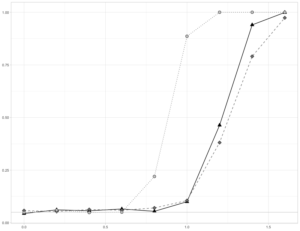
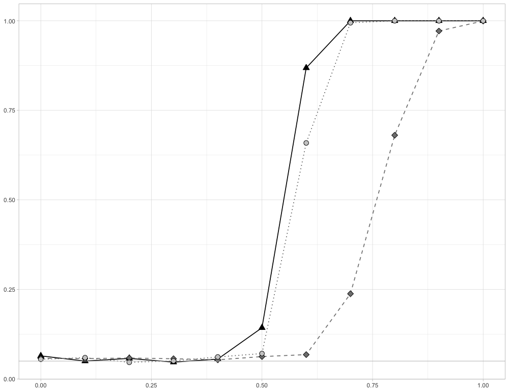
Figure 1: Simulated rejection probabilities of the test (3.6) under the null hypothesis ($\delta=0$) and the different alternatives in (3.8) (left) and (3.9) (right) for $\delta>0$ . The circle indicates $n=200,p=300$, the triangle $n=200,p=120$ and the square $n=150,p=300$.

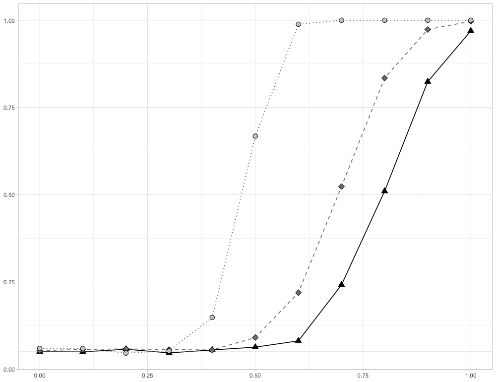
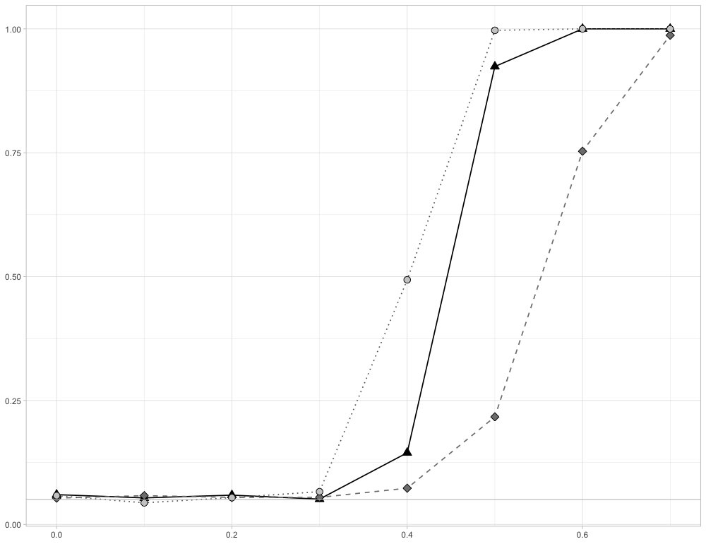
Figure 2: Simulated rejection probabilities of the test (3.6) under the null hypothesis ($\varepsilon=0$) and the different alternatives in (3.10) (left) and (3.11) (right) for $\varepsilon>0$. The circle indicates $n=200,p=300$, the triangle $n=200,p=120$ and the square $n=150,p=300$.

In Figure 1 and Figure 2, we display the the empirical rejection of the test (3.6) for the different alternatives and different values of $n$ and $p$, where the change point is given by $t^{\star}=0.6$. For the parameter $t_{0}$, we always use $t_{0}=0.2,$ and all results are based on $2,000$ simulation runs. The vertical grey line in each figure defines the nominal level $\alpha=5\%$.

Note that the choices $\delta=0$ and $\varepsilon=0$ correspond to the null hypothesis in (3.8), (3.9), (3.10) and (3.11), respectively. We observe a good approximation of the nominal level in all cases under consideration. Moreover, the test has power under all considered alternatives, even if the dimension $p$ is substantially larger than the sample size. Note that the test performs better for alternatives of the form (3.9) compared to the alternatives in (3.8). This reflects the intuition that the alternative in (3.8) is somehow closer to sphericity than the alternative (3.9). A similar observation can be made for the alternatives (3.10) and (3.11).

4 Proof of Theorem 2.1

4.1 Outline of the proof of Theorem 2.1

A frequently used powerful tool in random matrix theory is the Stieltjes transform. This is partially explained by the formula

$$\int f(x)dG(x) =\frac{1}{2\pi i}\int\int_{\mathcal{C}}\frac{f(z)}{z-x}dzdG(x)=-\frac{1}{2\pi i}\int_{\mathcal{C}}f(z)s_{G}(z)dz,$$ (4.1)

where $G$ is an arbitrary cumulative distribution function (c.d.f.) with a compact support, $f$ is an arbitrary analytic function on an open set, say $O$, containing the support of $G$, $\mathcal{C}$ is a positively oriented contour in $O$ enclosing the support of $G$ and

$$s_{G}(z)=\int\frac{1}{x-z}dG(x)$$

denotes the Stieltjes transform of $G$. Note that (4.1) follows from Cauchy’s integral and Fubini’s theorem. Thus invoking the continuous mapping theorem, it may suffice to prove weak convergence for the sequence $(M_{n})_{n\in\mathbb{N}}$, where

$$M_{n}(z,t)=p\left(s_{F^{\mathbf{B}_{n,t}}}(z)-s_{\tilde{F}^{y_{\lfloor nt\rfloor},H_{n}}}(z)\right),~{}~{}~{}{z\in\mathcal{C}}.$$ (4.2)

Here, $s_{\tilde{F}^{y_{\lfloor nt\rfloor},H_{n}}}$ denotes the Stieltjes transform of $\tilde{F}^{y_{\lfloor nt\rfloor},H_{n}}$ given in (2.7) characterized through the equation

$$s_{\tilde{F}^{y_{\lfloor nt\rfloor},H_{n}}}(z)=\int\frac{1}{\lambda\frac{\lfloor nt\rfloor}{n}\left(1-y_{\lfloor nt\rfloor}-y_{\lfloor nt\rfloor}zs_{\tilde{F}^{y_{\lfloor nt\rfloor},H_{n}}}(z)\right)-z}dH_{n}(\lambda),$$ (4.3)

and the contour $\mathcal{C}$ in (4.2) has to be constructed in such a way that it encloses the support of $\tilde{F}^{y_{\lfloor nt\rfloor},H_{n}}$ and $F^{\mathbf{B_{n,t}}}$ with probability $1$ for all $n\in\mathbb{N},t\in[t_{0},1]$. This idea is formalized in the proof of Theorem 2.1 in Section 4.2.

In order to prove the weak convergence of (4.2) define a contour $\mathcal{C}$ as follows. Let $x_{r}$ be any number greater than the right endpoint of the interval (2.8) and $v_{0}>0$ be arbitrary. Let $x_{l}$ be any negative number if the left endpoint of the interval (2.8) is zero. Otherwise, choose

$$x_{l}\in\left(0,\liminf\limits_{n\to\infty}\lambda_{\min}(\mathbf{T}_{n})I_{(0,1)}(y_{t_{0}})t_{0}(1-\sqrt{y_{t_{0}}})^{2}\right).$$

Let $\mathcal{C}_{u}=\{x+iv_{0}:x\in[x_{l},x_{r}]\}~{},$

$$\mathcal{C}^{+}=\{x_{l}+iv:v\in[0,v_{0}]\}~{}\cup~{}\mathcal{C}_{u}~{}\cup~{}\{x_{r}+iv:v\in[0,v_{0}]\}.$$

and define $\mathcal{C}=\mathcal{C}^{+}~{}\cup~{}\overline{\mathcal{C}^{+}}$, where $\overline{\mathcal{C}^{+}}$ contains all elements of $\mathcal{C}^{+}$ complex conjugated. Next, consider a sequence $(\varepsilon_{n})_{n\in\mathbb{N}}$ converging to zero such that for some $\alpha\in(0,1)$

$$\varepsilon_{n}\geq n^{-\alpha},$$

define

$$\mathcal{C}_{l} =\{x_{l}+iv:v\in[n^{-1}\varepsilon_{n},v_{0}]\}$$

$$\mathcal{C}_{r} =\{x_{r}+iv:v\in[n^{-1}\varepsilon_{n},v_{0}]\},$$

and consider the set $\mathcal{C}_{n}=\mathcal{C}_{l}\cup\mathcal{C}_{u}\cup\mathcal{C}_{r}$. We define an approximation $\hat{M}_{n}$ of the process ${M}_{n}$ for $z=x+iv\in\mathcal{C}^{+},t\in[t_{0},1]$ by

$$\hat{M}_{n}(z,t)=\begin{cases}M_{n}(z,t)&\textnormal{ if }z\in\mathcal{C}_{n},\\ M_{n}(x_{r}+in^{-1}\varepsilon_{n},t)&\textnormal{ if }x=x_{r},~{}v\in[0,n^{-1}\varepsilon_{n}],\\ M_{n}(x_{l}+in^{-1}\varepsilon_{n},t)&\textnormal{ if }x=x_{l},~{}v\in[0,n^{-1}\varepsilon_{n}].\end{cases}$$ (4.4)

In Lemma A.2 in the Appendix, it is shown that $(\hat{M}_{n})_{n\in\mathbb{N}}$ approximates $(M_{n})_{n\in\mathbb{N}}$ appropriately in the sense that the corresponding linear spectral statistics

$$-\frac{1}{2\pi i}\int_{\mathcal{C}}f(z)M_{n}(z,t)dz~{}~{}~{}~{}\textnormal{ and }-\frac{1}{2\pi i}\int_{\mathcal{C}}f(z)\hat{M}_{n}(z,t)dz~{}$$

in (4.1) coincide asymptotically. As a consequence the weak convergence of the process (4.2) follows from that of $\hat{M}_{n}$, which is established in the following theorem. The proof is given in Section 4.3.

Theorem 4.1 (Weak convergence for the process of Stieltjes transforms).

Under the assumptions of Theorem 2.1, the sequence $(\hat{M}_{n})_{n\in\mathbb{N}}$ defined in (4.4) converges weakly to a Gaussian process $(M(z,t))_{z\in\mathcal{C}^{+},t\in[t_{0},1]}$ in the space $\ell^{\infty}(\mathcal{C}^{+}\times[t_{0},1])$.

The mean of the limiting process $M$ is given by

$$\mathbb{E}M(z,t)=\begin{cases}\frac{ty\int\frac{\tilde{\underline{s}}_{t}^{3}(z)\lambda^{2}}{(t\tilde{\underline{s}}_{t}(z)\lambda+1)^{3}}dH(\lambda)}{\left(1-ty\int\frac{\tilde{\underline{s}}_{t}^{2}(z)\lambda^{2}}{(t\tilde{\underline{s}}_{t}(z)\lambda+1)^{2}}dH(\lambda)\right)^{2}}&\textnormal{ for the real case,}\\ 0&\textnormal{ for the complex case}\end{cases}$$ (4.5)

($z\in\mathcal{C}^{+}$, $t\in[t_{0},1]$). In the complex case the covariance kernel of the limiting process $M$ is given by

$$\operatorname{cov}(M(z_{1},t_{1}),M(z_{2},t_{2}))=\sigma_{t_{1},t_{2}}^{2}(z_{1},\overline{z_{2}}),$$

where $\sigma_{t_{1},t_{2}}^{2}(z_{1},z_{2})$ is defined in (4.19). In the real case, we have

$$\operatorname{cov}(M(z_{1},t_{1}),M(z_{2},t_{2}))=2\sigma_{t_{1},t_{2}}^{2}(z_{1},\overline{z_{2}}).$$ (4.6)

4.2 Proof of Theorem 2.1 using Theorem 4.1

From (4.1) we obtain

$$-\frac{1}{2\pi i}\int\limits_{\mathcal{C}}f(z)\mathbb{E}s_{G}(z)dz=-\frac{1}{2\pi i}\mathbb{E}\int\limits_{\mathcal{C}}f(z)s_{G}(z)dz=\mathbb{E}\int f(x)dG(x).$$ (4.7)

We choose $v_{0},x_{r},x_{l}$ so that $f_{1}$ and $f_{2}$ given in Theorem 2.1 are analytic on and inside the resulting contour $\mathcal{C}$ and define

$$\mathbf{S}_{n,t}=\frac{1}{n}\mathbf{X}_{n,t}\mathbf{X}_{n,t}^{\star}.$$

The almost sure convergence

$$\lim\limits_{n\to\infty}\lambda_{\min}(\mathbf{S}_{n,t}) =t(1-\sqrt{y_{t}})^{2}I_{(0,1)}(y_{t})=(\sqrt{t}-\sqrt{y})^{2}I_{(0,1)}(y_{t}),$$

$$~{}\lim\limits_{n\to\infty}\lambda_{\max}(\mathbf{S}_{n,t}) =t(1+\sqrt{y_{t}})^{2}=(\sqrt{t}+\sqrt{y})^{2}$$

of the extreme eigenvalues (see, e.g., Theorem 1.1 in Bai and Zhou, , 2008) and the inequalities

$$\lambda_{\max}(\mathbf{AB})\leq\lambda_{\max}(\mathbf{A})\lambda_{\max}(\mathbf{B}),~{}\lambda_{\min}(\mathbf{AB})\geq\lambda_{\min}(\mathbf{A})\lambda_{\min}(\mathbf{B})$$

(valid for quadratic Hermitian nonnegative definite matrices $\mathbf{A}$ and $\mathbf{B}$) imply

$$\limsup\limits_{n\to\infty}\lambda_{\max}(\mathbf{B}_{n,t}) \leq\limsup\limits_{n\to\infty}\lambda_{\max}(\mathbf{T}_{n})\cdot\limsup\limits_{n\to\infty}\lambda_{\max}(\mathbf{S}_{n,t})\ =\limsup\limits_{n\to\infty}\lambda_{\max}(\mathbf{T}_{n})t\left(1+\sqrt{y_{t}}\right)^{2}$$

$$\leq\limsup\limits_{n\to\infty}\lambda_{\max}(\mathbf{T}_{n})\left(1+\sqrt{y_{t_{0}}}\right)^{2}<x_{r}$$

for each $t\in[t_{0},1]$ with probability $1$. Similar calculations for $x_{l}$ show that it holds for all $t\in[t_{0},1]$ with probability 1

$$\liminf\limits_{n\to\infty}\min\big{(}x_{r}-\lambda_{\max}(\mathbf{B}_{n,t}),\lambda_{\min}(\mathbf{B}_{n,t})-x_{l}\big{)}>0,$$ (4.8)

which implies that for sufficiently large $n$ the contour $\mathcal{C}$ encloses the support of $F^{\mathbf{B}_{n,t}}$, $t\in[t_{0},1]$, with probability $1$ for (note that the null set depends on $n$ and $t$). For every $n$, there exist only finitely many $t_{1},t_{2}\in[t_{0},1]$ such that $\lfloor nt_{1}\rfloor\neq\lfloor nt_{2}\rfloor$. Since the countable union of null sets is again a null set, we may choose the above nullset in such a way that $\mathcal{C}$ encloses the support of $F^{\mathbf{B}_{n,t}}$ for sufficiently large $n$ with probability 1 (this null set independent of $n$ and $t\in[t_{0},1]$). From Lemma A.1 in the Appendix, it follows that the support of $\tilde{F}^{y_{\lfloor nt\rfloor},H_{n}}$, $t\in[t_{0},1]$, is contained in the interval

$$\Big{[}\frac{\lfloor nt_{0}\rfloor}{n}\lambda_{\min}(\mathbf{T}_{n})I_{(0,1)}(y_{\lfloor nt_{0}\rfloor})(1-\sqrt{y_{\lfloor nt_{0}\rfloor}})^{2},\lambda_{\max}(\mathbf{T}_{n})(1+\sqrt{y_{\lfloor nt_{0}\rfloor}})^{2}\Big{]},$$

which is enclosed by the contour $\mathcal{C}$ for sufficiently large $n$. Therefore, using (4.1) and (4.7), we have almost surely

$$\Big{(}\Big{(}-\frac{1}{2\pi i}\int_{\mathcal{C}}f_{i}(z)M_{n}(z,t)dz\Big{)}_{i=1,2}\Big{)}_{t\in[t_{0},1]}=\big{(}(X_{n}(f_{i},t))_{i=1,2}\big{)}_{t\in[t_{0},1]}$$

for sufficiently large $n$. Moreover, we have with probability 1 (see Lemma A.2 in the Appendix)

$$\Big{|}\int\limits_{\mathcal{C}}f_{i}(z)(M_{n}(z,t)-\hat{M}_{n}(z,t))dz\Big{|}=o(1),~{}i=1,2,$$

uniformly with respect to $t\in[t_{0},1]$. Let $C(\mathcal{C}\times[t_{0},1])$ and $C([t_{0},1])$ denote the spaces of continuous functions defined on $\mathcal{C}\times[t_{0},1]$ and $[t_{0},1]$, respectively, then the mapping

$$C(\mathcal{C}\times[t_{0},1])\to\left(C([t_{0},1])\right)^{2},~{}h\mapsto\left(I_{f_{1}}(h),I_{f_{2}}(h)\right)$$

is continuous, where

$$I_{f_{i}}(h)(\cdot)=-\frac{1}{2\pi i}\int_{\mathcal{C}}f(z)h(z,\cdot)dz\in C([t_{0},1]),i=1,2.$$

By Corollary 4.1 stated in Section 4.3.3 below and (4.5), the limiting process $M$ in Theorem 4.1 satisfies $M\in C(\mathcal{C}^{+}\times[t_{0},1])$. Invoking the continuous mapping theorem (see Theorem 1.3.6 in Van Der Vaart and Wellner, , 1996) and noting that $\overline{M_{n}(z,t)}=M_{n}(\overline{z},t)$, we have

$$\big{(}I_{f_{1}}(\hat{M}_{n}),I_{f_{2}}(\hat{M}_{n})\big{)} \rightsquigarrow\left(I_{f_{1}}(M),I_{f_{2}}(M)\right)=\Big{(}\Big{(}-\frac{1}{2\pi i}\int_{\mathcal{C}}f_{i}(z)M(z,t)dz\Big{)}_{i=1,2}~{}\Big{)}_{t\in[t_{0},1]}.$$

The fact that this random variable is a Gaussian process follows from the observation that the Riemann sums corresponding to these integrals are multivariate Gaussian and therefore integral must be Gaussian as well. The limiting expression for the mean and the covariance follow immediately from Theorem 4.1. For example, we have for the real case observing (4.6)

$$\operatorname{cov}\Big{(}-\frac{1}{2\pi i}\int_{\mathcal{C}}f_{1}(z)M(z,t_{1})dz,-\frac{1}{2\pi i}\int_{\mathcal{C}}f_{2}(z)M(z,t_{2})dz\Big{)}$$

$$= \frac{1}{4\pi^{2}}\int_{\mathcal{C}_{1}}\int_{\mathcal{C}_{2}}f_{1}(z_{1})\overline{f_{2}(z_{2})}\operatorname{cov}\left(M(z_{1},t_{1}),M(z_{2},t_{2})\right)\overline{dz_{2}}dz_{1}$$

$$= \frac{1}{2\pi^{2}}\int_{\mathcal{C}_{1}}\int_{\mathcal{C}_{2}}f_{1}(z_{1})\overline{f_{2}(z_{2})}\sigma_{t_{1},t_{2}}^{2}(z_{1},\overline{z_{2}})\overline{dz_{2}}dz_{1}.$$

4.3 Proof of Theorem 4.1

We begin with the usual “truncation” and replace the entries of the matrix $\mathbf{X}_{n}=(x_{ij})_{i=1,...,p,j=1,...,n}$ by truncated variables [see Section 9.7.1, Bai and Silverstein, (2010)]. More precisely, without loss of generality we assume that

$$|x_{ij}|<\eta_{n}\sqrt{n},~{}\mathbb{E}[x_{ij}]=0,~{}\mathbb{E}|x_{ij}|^{2}=1,~{}\mathbb{E}|x_{ij}|^{4}<\infty.$$

Additionally, for the real case (part (1) of Theorem 2.1) we may assume that

$$\mathbb{E}|x_{ij}|^{4}=3+o(1)$$

uniformly in $i\in\{1,\ldots,p\},j\in\{1,\ldots,n\}$, and for the complex case (part (2) of Theorem 2.1)

$$\mathbb{E}x_{ij}^{2}=o\Big{(}\frac{1}{n}\Big{)},~{}\mathbb{E}|x_{ij}|^{4}=2+o(1)$$

uniformly in $i\in\{1,\ldots,p\},j\in\{1,\ldots,n\}$. Here, $(\eta_{n})_{n\in\mathbb{N}}$ denotes a sequence converging to zero with the property

$$\eta_{n}n^{{1}/{5}}\to\infty.$$

We now give a brief outline for the proof of Theorem 4.1 describing the important steps, which are carried out in the following sections and the online appendix. We consider the stochastic processes $(M_{n})_{n\in\mathbb{N}}$ and $(\hat{M}_{n})_{n\in\mathbb{N}}$ (which is defined in (4.4)) as sequences in the space $\ell^{\infty}(\mathcal{C}^{+}\times[t_{0},1])$ and use the decomposition

$$M_{n}=M_{n}^{1}+M_{n}^{2}~{},$$ (4.9)

where the random part $M_{n}^{1}$ and the deterministic part $M_{n}^{2}$ are given by

$$M_{n}^{1}(z,t)= p\left(s_{F^{\mathbf{B}_{n,t}}}(z)-\mathbb{E}\left[s_{F^{\mathbf{B}_{n,t}}}(z)\right]\right),$$ (4.10)

$$M_{n}^{2}(z,t)= p\left(\mathbb{E}\left[s_{F^{\mathbf{B}_{n,t}}}(z)\right]-s_{\tilde{F}^{y_{\lfloor nt\rfloor},H_{n}}}(z)\right),~{}$$ (4.11)

the Stieltjes transform $s_{\tilde{F}^{y_{\lfloor nt\rfloor},H_{n}}}$ is defined in (4.3) and $s_{F^{\mathbf{B}_{n,t}}}$ denotes the Stieltjes transform of the empirical spectral distribution $F^{\mathbf{B}_{n,t}}.$
Our first result provides the convergence of the finite-dimensional distributions of $({M}_{n}^{1})_{n\in\mathbb{N}}$. Its proof relies on a central limit theorem for martingale difference schemes and is carried out in Section 4.3.2.

Theorem 4.2.

Under the assumption (1) for the real case or assumption (2) for the complex case from Theorem 2.1, it holds for all $k\in\mathbb{N},t_{1},t_{2}\in[0,1]$, $z_{1},...,z_{k}\in\mathbb{C}$, $\operatorname{Im}(z_{i})\neq 0$

$$(M_{n}^{1}(z_{1},t_{1}),M_{n}^{1}(z_{1},t_{2}),...,M_{n}^{1}(z_{k},t_{1}),M_{n}^{1}(z_{k},t_{2}))^{\top}$$

$$\stackrel{{\scriptstyle\mathcal{D}}}{{\to}}(M^{1}(z_{1},t_{1}),M^{1}(z_{1},t_{2}),...,M^{1}(z_{k},t_{1}),M^{1}(z_{k},t_{2}))^{\top}~{},$$ (4.12)

where $M^{1}(z,t)=M(z,t)-\mathbb{E[}M(z,t)]$ is the centered version of the Gaussian process defined in Theorem 4.1.

Next, we define the process $\hat{M}_{n}^{1}$ in the same way as $\hat{M}_{n}$ in (4.4) replacing $M_{n}$ by $M_{n}^{1}$ and show the following tightness result. The main argument in in its proof consists in establishing delicate moment inequalities for the increments of the process $(\hat{M}_{n}^{1})_{n\in\mathbb{N}}$, see Lemma 4.1 and its proof in Appendix B.1.

Theorem 4.3.

Under the assumptions of Theorem 2.1, the sequence $(\hat{M}_{n}^{1})_{n\in\mathbb{N}}$ is asymptotically tight in the space $\ell^{\infty}(\mathcal{C}^{+}\times[t_{0},1])$.

The third step is an investigation of the deterministic part. In particular we show that the bias $(M_{n}^{2})_{n\in\mathbb{N}}$ converges in the space $\ell^{\infty}(\mathcal{C}^{+}\times[t_{0},1])$ to the limit given in (4.5). Note that the space of bounded function is equipped with the sup-norm, which demands an uniform convergence of the Stieltjes transform $\mathbb{E}[s_{F^{\mathbf{B}_{n,t}}}(z)]$ with respect to the arguments $t\in[t_{0},1],z\in\mathcal{C}^{+}.$ The latter result is provided in Theorem 4.5 in Section 4.3.4.

Theorem 4.4.

Under the assumptions of Theorem 2.1, it holds

$$\lim\limits_{n\to\infty}\sup\limits_{\begin{subarray}{c}z\in\mathcal{C}_{n},\\ t\in[t_{0},1]\end{subarray}}\left|M_{n}^{2}(z,t)-\mathbb{E}[M(z,t)]\right|=0.$$

The proofs of Theorem 4.2, 4.3 and 4.4 are postponed to Section 4.3.2, 4.3.3 and 4.3.4, respectively. Using these results, we are now in the position to prove Theorem 4.1.

4.3.1 Proof of Theorem 4.1

Theorem 4.2 yields the convergence of the finite-dimensional distributions of $M_{n}^{1}(z,t)$ for $t\in[t_{0},1]$ and $z\in\mathcal{C}$ with $\operatorname{Im}(z)\neq 0$ towards the corresponding finite-dimensional distributions of the centered process $M^{1}(z,t)=M(z,t)-\mathbb{E}[M(z,t)]$. By the definition in equation (4.4), this implies the convergence of the finite-dimensional distributions of $\hat{M}_{n}^{1}(z,t)$ for $t\in[t_{0},1]$ and $z\in\mathcal{C}$ with $\operatorname{Im}(z)\neq 0$ towards the corresponding finite-dimensional distributions of $M^{1}$. Since the limiting process $(M^{1}(z,t))_{z\in\mathcal{C}^{+},t\in[t_{0},1]}$ is continuous as proven later in this section (see Corollary 4.1 in Section 4.3.3) and $\left(\mathcal{C}^{+}\setminus\{x_{l},x_{r}\}\right)\times[t_{0},1]$ is a dense subset of $\mathcal{C}^{+}\times[t_{0},1]$, this is sufficient in order to ensure uniqueness of the limiting process. As Theorem 4.3 establishes tightness, Theorem 4.1 follows from the decomposition (4.9), Theorem 1.5.6 in Van Der Vaart and Wellner, (1996) and Theorem 4.4.

4.3.2 Proof of Theorem 4.2

We start by performing some preparations and by introducing notations which will remain crucial for the rest of this work. Using the Cramér–Wold device, the convergence in (4.12) is equivalent to the weak convergence

$$\sum\limits_{i=1}^{k}\left(\alpha_{i,1}M_{n}^{1}(z_{i},t_{1})+\alpha_{i,2}(M_{n}^{1}(z_{i},t_{2})\right)\stackrel{{\scriptstyle\mathcal{D}}}{{\to}}\sum\limits_{i=1}^{k}\left(\alpha_{i,1}M^{1}(z_{i},t_{1})+\alpha_{i,2}(M^{1}(z_{i},t_{2})\right)$$ (4.13)

for all $\alpha_{1,1},\ldots,\alpha_{k,1},\alpha_{1,2},\ldots,\alpha_{k,2}\in\mathbb{C}$. We want to show that the limiting random variable on the right hand side of the display above follows a Gaussian distribution under the assumption (1) or (2) of Theorem 2.1.
Recalling assumption (b) in Theorem 2.1, we may assume $||\mathbf{T}_{n}||\leq 1$, $n\in\mathbb{N}$. Define for $k,j=1,..,\lfloor nt\rfloor$, $k\neq j$, $t\in(0,1]$, $z\in\mathbb{C}$ with Im$(z)\neq 0$

$$\mathbf{r}_{j} =\frac{1}{\sqrt{n}}\mathbf{T}_{n}^{\frac{1}{2}}\mathbf{x}_{j}$$

$$\mathbf{B}_{n,t} =\sum\limits_{j=1}^{\lfloor nt\rfloor}\mathbf{r}_{j}\mathbf{r}_{j}^{\star},$$

$$\mathbf{D}_{t}(z) =\mathbf{B}_{n,t}-z\mathbf{I},$$

$$\mathbf{D}_{j,t}(z) =\mathbf{D}_{t}(z)-\mathbf{r}_{j}\mathbf{r}_{j}^{\star},$$

$$\mathbf{D}_{k,j,t}(z) =\mathbf{D}_{j,t}(z)-\mathbf{r}_{k}\mathbf{r}_{k}^{\star}=\mathbf{D}_{t}(z)-\mathbf{r}_{k}\mathbf{r}_{k}^{\star}-\mathbf{r}_{j}\mathbf{r}_{j}^{\star},$$

$$\alpha_{j,t}(z) =\mathbf{r}_{j}^{\star}\mathbf{D}_{j,t}^{-2}(z)\mathbf{r}_{j}-n^{-1}\operatorname{tr}(\mathbf{D}_{j,t}^{-2}(z)\mathbf{T}_{n}),$$

$$\gamma_{j,t}(z) =\mathbf{r}_{j}^{\star}\mathbf{D}_{j,t}^{-1}(z)\mathbf{r}_{j}-n^{-1}\mathbb{E}\operatorname{tr}(\mathbf{D}_{j,t}^{-1}(z)\mathbf{T}_{n}),$$

$$\gamma_{k,j,t}(z) =\mathbf{r}_{k}^{\star}\mathbf{D}_{k,j,t}^{-1}(z)\mathbf{r}_{k}-n^{-1}\mathbb{E}\left[\operatorname{tr}\left(\mathbf{T}_{n}\mathbf{D}_{k,j,t}^{-1}(z)\right)\right]$$

$$\hat{\gamma}_{j,t}(z) =\mathbf{r}_{j}^{\star}\mathbf{D}_{j,t}^{-1}(z)\mathbf{r}_{j}-n^{-1}\operatorname{tr}(\mathbf{D}_{j,t}^{-1}(z)\mathbf{T}_{n}),$$

$$\beta_{j,t}(z) =\frac{1}{1+\mathbf{r}_{j}^{\star}\mathbf{D}_{j,t}^{-1}(z)\mathbf{r}_{j}},$$

$$\beta_{k,j,t}(z) =\frac{1}{1+\mathbf{r}_{k}^{\star}\mathbf{D}_{k,j,t}^{-1}(z)\mathbf{r}_{k}},$$

$$\overline{\beta}_{j,t}(z) =\frac{1}{1+n^{-1}\operatorname{tr}(\mathbf{T}_{n}\mathbf{D}_{j,t}^{-1}(z))},$$

$$b_{j,t}(z) =\frac{1}{1+n^{-1}\mathbb{E}\operatorname{tr}(\mathbf{T}_{n}\mathbf{D}_{j,t}^{-1}(z))},$$

$$b_{t}(z) =\frac{1}{1+n^{-1}\mathbb{E}\operatorname{tr}(\mathbf{T}_{n}\mathbf{D}_{t}^{-1}(z))}.$$

Note that the terms $\beta_{j,t}(z),\beta_{k,j,t}(z),\overline{\beta}_{j,t}(z),b_{j,t}(z)$ and $b_{t}(z)$ are bounded in absolute value by $|z|/v$, where $v={\rm Im}(z)$ is assumed to be positive (see (6.2.5) in Bai and Silverstein, , 2010). By the Sherman–Morrison formula we obtain the representation

$$\mathbf{D}_{t}^{-1}(z)-\mathbf{D}_{j,t}^{-1}(z)=-\mathbf{D}_{j,t}^{-1}(z)\mathbf{r}_{j}\mathbf{r}_{j}^{\star}\mathbf{D}_{j,t}^{-1}(z)\beta_{j,t}(z).$$ (4.14)

In order to prove asymptotic normality of the random variable appearing in (4.13), we show that it can be represented as a suitable martingale difference scheme plus some negligible remainder, which allows us to apply a central limit theorem.
For $j=1\ldots,n$ let $\mathbb{E}_{j}$ denote the conditional expectation with respect to the filtration $\mathcal{F}_{nj}=\sigma(\{\mathbf{r}_{1},...,\mathbf{r}_{j}\})$ (by $\mathbb{E}_{0}$ we denote the common expectation). Recalling the definition (4.10) and using the martingale decomposition, we have

$$M_{n}^{1}(z,t) =\operatorname{tr}(\mathbf{D}_{t}^{-1}(z)-\mathbb{E}\mathbf{D}_{t}^{-1}(z))$$

$$=\sum\limits_{j=1}^{\lfloor nt\rfloor}\left(\operatorname{tr}\mathbb{E}_{j}\mathbf{D}_{t}^{-1}(z)-\operatorname{tr}\mathbb{E}_{j-1}\mathbf{D}_{t}^{-1}(z)\right)$$

$$=\sum\limits_{j=1}^{\lfloor nt\rfloor}\left(\operatorname{tr}\mathbb{E}_{j}\left[\mathbf{D}_{t}^{-1}(z)-\mathbf{D}_{t,j}^{-1}(z)\right]-\operatorname{tr}\mathbb{E}_{j-1}\left[\mathbf{D}_{t}^{-1}(z)-\mathbf{D}_{j,t}^{-1}(z)\right]\right)$$

$$=-\sum\limits_{j=1}^{\lfloor nt\rfloor}(\mathbb{E}_{j}-\mathbb{E}_{j-1})\beta_{j,t}(z)\mathbf{r}_{j}^{\star}\mathbf{D}_{j,t}^{-2}(z)\mathbf{r}_{j}.$$ (4.15)

Since, from now on, the proof is similar in spirit to Section 9.9 in Bai and Silverstein, (2010), we restrict ourselves to an overview explaining the main steps and important differences. By similar arguments as given in this monograph it can be shown, that it is sufficient to prove asymptotic normality for the quantity

$$\sum\limits_{j=1}^{\max(\lfloor nt_{1}\rfloor,\lfloor nt_{2}\rfloor)}Z_{nj}^{t_{1},t_{2}}~{},$$

where

$$Z_{nj}^{t_{1},t_{2}} =\sum\limits_{i=1}^{k}\left(\alpha_{i,1}Y_{j,t_{1}}(z_{i})+\alpha_{i,2}Y_{j,t_{2}}(z_{i})\right)~{},$$

$$Y_{j,t}(z) =-\mathbb{E}_{j}\Big{[}\overline{\beta}_{j,t}(z)\alpha_{j,t}(z)-\overline{\beta}_{j,t}^{2}(z)\hat{\gamma}_{j,t}(z)\frac{1}{n}\operatorname{tr}(\mathbf{T}_{n}\mathbf{D}_{j,t}^{-2}(z))\Big{]}=-\mathbb{E}_{j}\frac{d}{dz}\overline{\beta}_{j,t}(z)\hat{\gamma}_{j,t}(z)~{}$$

if $j\leq\lfloor nt\rfloor$ and $Y_{j,t}(z)=0$ if $j>\lfloor nt\rfloor$.

For this purpose we verify conditions (5.29) - (5.31) of the central limit theorem for complex-valued martingale difference schemes given in Lemma 5.6 of Najim and Yao, (2016). It is straightforward to show that $Z_{nj}^{t_{1},t_{2}}$ forms a martingale difference scheme with respect to to the filtration $\mathcal{F}_{nj}=\sigma(\{\mathbf{r}_{1},...,\mathbf{r}_{j}\})$ and we can prove that (5.31) in this reference holds true by deriving bounds for the $4$th moment of $Y_{j,t}(z)$. For a proof of condition (5.30), we note that

$$\sum\limits_{j=1}^{\max(\lfloor nt_{1}\rfloor,\lfloor nt_{2}\rfloor)}\mathbb{E}_{j-1}\left[\left(Z_{nj}^{t_{1},t_{2}}\right)^{2}\right]= \sum\limits_{i,l=1}^{k}\Big{(}\sum\limits_{j=1}^{\lfloor nt_{1}\rfloor}\alpha_{i,1}\alpha_{l,1}\mathbb{E}_{j-1}[Y_{j,t_{1}}(z_{i})Y_{j,t_{1}}(z_{l})]$$

$$+\sum\limits_{j=1}^{\min(\lfloor nt_{1}\rfloor,\lfloor nt_{2}\rfloor)}\alpha_{i,1}\alpha_{l,2}\mathbb{E}_{j-1}[Y_{j,t_{1}}(z_{i})Y_{j,t_{2}}(z_{l})]$$

$$+\sum\limits_{j=1}^{\min(\lfloor nt_{1}\rfloor,\lfloor nt_{2}\rfloor)}\alpha_{i,2}\alpha_{l,1}\mathbb{E}_{j-1}[Y_{j,t_{2}}(z_{i})Y_{j,t_{1}}(z_{l})]$$

$$+\sum\limits_{j=1}^{\lfloor nt_{2}\rfloor}\alpha_{i,2}\alpha_{l,2}\mathbb{E}_{j-1}[Y_{j,t_{2}}(z_{i})Y_{j,t_{2}}(z_{l})]\Big{)}~{}.$$

As all terms have the same form, it is sufficient to show that for all $z_{1},z_{2}\in\mathbb{C}$ with $\textnormal{Im}(z_{1}),\textnormal{Im}(z_{2})\neq 0$ and $t_{1},t_{2}\in(0,1]$

$$V_{n}(z_{1},z_{2},t_{1},t_{2})=\sum\limits_{j=1}^{\min(\lfloor nt_{1}\rfloor,\lfloor nt_{2}\rfloor)}\mathbb{E}_{j-1}\left[Y_{j,t_{1}}(z_{1})Y_{j,t_{2}}(z_{2})\right]~{}~{}\stackrel{{\scriptstyle\mathbb{P}}}{{\to}}~{}\sigma_{t_{1},t_{2}}^{2}(z_{1},{z_{2}})$$ (4.16)

for an appropriate function $\sigma_{t_{1},t_{2}}^{2}(z_{1},z_{2})$ (see equation (4.19) below for a precise definition). Note that this convergence implies condition (5.29), since

$$\sum\limits_{j=1}^{\min(\lfloor nt_{1}\rfloor,\lfloor nt_{2}\rfloor)}\mathbb{E}_{j-1}\big{[}Y_{j,t_{1}}(z_{1})\overline{Y_{j,t_{2}}(z_{2})}\big{]}=\sum\limits_{j=1}^{\min(\lfloor nt_{1}\rfloor,\lfloor nt_{2}\rfloor)}\mathbb{E}_{j-1}\left[Y_{j,t_{1}}(z_{1})Y_{j,t_{2}}(\overline{z_{2}})\right]\stackrel{{\scriptstyle\mathbb{P}}}{{\to}}~{}\sigma_{t_{1},t_{2}}^{2}(z_{1},\overline{z_{2}}),$$

where the equality follows from the fact that the matrices $\mathbf{T}_{n},\mathbf{B}_{n,t},\mathbf{r}_{j}\mathbf{r}_{j}^{\star}$ are Hermitian and $(\overline{\mathbf{D}_{j,t}^{-1}(z)})^{T}=\mathbf{D}_{j,t}^{-1}(\overline{z}).$ Consequently, Lemma 5.6 in Najim and Yao, (2016) combined with the Cramér–Wold device yields the weak convergence of the finite-dimensional distributions to a multivariate normal distribution with covariance $\sigma_{t_{1},t_{2}}^{2}(z_{1},\overline{z_{2}})=\operatorname{cov}(M^{1}(z_{1},t_{1}),M^{1}(z_{2},t_{2}))$.

Hence, it is remains to show (4.16) in order to establish the convergence of the finite dimensional distributions. For this purpose, we introduce the quantity

$$V_{n}^{(2)}(z_{1},z_{2},t_{1},t_{2}) =\frac{1}{n^{2}}\sum\limits_{j=1}^{\min(\lfloor nt_{1}\rfloor,\lfloor nt_{2}\rfloor)}b_{j,t_{1}}(z_{1})b_{j,t_{2}}(z_{2})\operatorname{tr}\left(\mathbb{E}_{j}\left[\mathbf{D}_{j,t_{1}}^{-1}(z_{1})\right]\mathbf{T}_{n}\mathbb{E}_{j}\left[\mathbf{D}_{j,t_{2}}^{-1}(z_{2})\right]\mathbf{T}_{n}\right),$$

and note that it can be shown by similar arguments as on p. $273$ in Bai and Silverstein, (2010) that

$$\frac{\partial^{2}}{\partial z_{1}\partial z_{2}}V_{n}^{(2)}(z_{1},z_{2},t_{1},t_{2})=V_{n}(z_{1},z_{2},t_{1},t_{2})+o_{\mathbb{P}}(1)~{}.$$ (4.17)

Moreover, we can show

$$V_{n}^{(2)}(z_{1},z_{2},t_{1},t_{2})\stackrel{{\scriptstyle\mathbb{P}}}{{\to}}a(z_{1},z_{2},t_{1},t_{2})\int\limits_{0}^{\min(t_{1},t_{2})}\frac{1}{1-\lambda a(z_{1},z_{2},t_{1},t_{2})}d\lambda,~{}n\to\infty,$$ (4.18)

where

$$a(z_{1},z_{2},t_{1},t_{2}) =\frac{\tilde{\underline{s}}_{t_{2}}(z_{2})-\tilde{\underline{s}}_{t_{1}}(z_{1})+(z_{1}-z_{2})\tilde{\underline{s}}_{t_{1}}(z_{1})\tilde{\underline{s}}_{t_{2}}(z_{2})}{t_{2}\tilde{\underline{s}}_{t_{2}}(z_{2})-t_{1}\tilde{\underline{s}}_{t_{1}}(z_{1})}$$

and the Stieltjes transform $\tilde{\underline{s}}_{t}(z)$ is defined in (2.4). From (4.17) and (4.18) it follows that

$$\sigma_{t_{1},t_{2}}^{2}(z_{1},z_{2}) =\frac{\partial^{2}}{\partial z_{1}\partial z_{2}}\int\limits_{0}^{\min(t_{1},t_{2})a(z_{1},z_{2},t_{1},t_{2})}\frac{1}{1-\lambda}d\lambda=\frac{\partial}{\partial z_{2}}\Big{(}\frac{\min(t_{1},t_{2})\frac{\partial}{\partial z_{1}}a(z_{1},z_{2},t_{1},t_{2})}{1-\min(t_{1},t_{2})a(z_{1},z_{2},t_{1},t_{2})}\Big{)}$$

$$=\frac{\textnormal{numerator}}{\textnormal{denominator}},$$ (4.19)

where

$$\textnormal{numerator}= \min(t_{1},t_{2})\Big{\{}-t_{2}(t_{2}-\min(t_{1},t_{2}))\tilde{\underline{s}}_{t_{2}}^{2}(z_{2})\tilde{\underline{s}}_{t_{1}}^{\prime}(z_{1})\Big{[}t_{2}\tilde{\underline{s}}_{t_{2}}^{2}(z_{2})+(t_{1}-t_{2})\tilde{\underline{s}}_{t_{2}}^{\prime}(z_{2})\Big{]}\Big{\}}$$

$$-t_{1}^{2}\tilde{\underline{s}}_{t_{1}}^{4}(z_{1})\Big{\{}\min(t_{1},t_{2})\tilde{\underline{s}}_{t_{2}}^{2}(z_{2})+(t_{1}-\min(t_{1},t_{2})\tilde{\underline{s}}_{t_{2}}^{\prime}(z_{2}))\Big{\}}$$

$$+2t_{1}t_{2}\tilde{\underline{s}}_{t_{1}}^{3}(z_{1})\tilde{\underline{s}}_{t_{2}}(z_{2})\Big{\{}\min(t_{1},t_{2})\tilde{\underline{s}}_{t_{2}}^{2}(z_{2})+(t_{1}-\min(t_{1},t_{2}))\tilde{\underline{s}}_{t_{2}}^{\prime}(z_{2})\Big{\}}$$

$$+2t_{1}t_{2}(t_{2}-\min(t_{1},t_{2}))\tilde{\underline{s}}_{t_{1}}(z_{1})\tilde{\underline{s}}_{t_{2}}^{2}(z_{2})\tilde{\underline{s}}_{t_{1}}^{\prime}(z_{1})\Big{\{}\tilde{\underline{s}}_{t_{2}}(z_{2})+(-z_{1}+z_{2})\tilde{\underline{s}}_{t_{2}}^{\prime}(z_{2})\Big{\}}$$

$$+\tilde{\underline{s}}_{t_{1}}^{2}(z_{1})\Big{\{}-t_{2}^{2}\min(t_{1},t_{2})\tilde{\underline{s}}_{t_{2}}^{4}(z_{2})+t_{1}(t_{1}-t_{2})(t_{1}-\min(t_{1},t_{2}))\tilde{\underline{s}}_{t_{1}}^{\prime}(z_{1})\tilde{\underline{s}}_{t_{2}}^{\prime}(z_{2})$$

$$+2t_{1}t_{2}(t_{1}-\min(t_{1},t_{2}))(z_{1}-z_{2})\tilde{\underline{s}}_{t_{2}}(z_{2})\tilde{\underline{s}}_{t_{1}}^{\prime}(z_{1})\tilde{\underline{s}}_{t_{2}}^{\prime}(z_{2})$$

$$+\tilde{\underline{s}}_{t_{2}}^{2}(z_{2})\Big{[}t_{2}^{2}(-t_{1}+\min(t_{1},t_{2}))\tilde{\underline{s}}_{t_{2}}^{\prime}(z_{2})$$

$$+t_{1}\tilde{\underline{s}}_{t_{1}}^{\prime}(z_{1})\Big{(}t_{1}(-t_{2}+\min(t_{1},t_{2}))+t_{2}\min(t_{1},t_{2})(z_{1}-z_{2})^{2}\tilde{\underline{s}}_{t_{2}}^{\prime}(z_{2})\Big{)}\Big{]}\Big{\}}$$

$$\textnormal{denominator}= \left(t_{1}\tilde{\underline{s}}_{t_{1}}(z_{1})-t_{2}\underline{s}_{t_{2}}(z_{2})\right)^{2}\Big{\{}(-t_{2}+\min(t_{1},t_{2}))\tilde{\underline{s}}_{t_{2}}(z_{2})$$

$$+\tilde{\underline{s}}_{t_{1}}(z_{1})(t_{1}-\min(t_{1},t_{2})+\min(t_{1},t_{2})(z_{1}-z_{2})\tilde{\underline{s}}_{t_{2}}(z_{2}))\Big{\}}^{2}.$$

The proofs of (4.17) and (4.18) are very similar to Bai and Silverstein, (2010) and omitted for the sake of brevity. Note also, that for the special case $t_{1}=t_{2}=1$, this covariance structure coincides with formula (9.8.4) in this monograph.

4.3.3 Proof of Theorem 4.3 and continuity of the limiting process

We will show that the assumptions of Corollary A.4 in Dette and Tomecki, (2019) are satisfied, where we identify the curve $\mathcal{C}^{+}$ with the compact interval $[0,1]$. For this purpose, we define the increments for the first and second coordinate of $\hat{M}_{n}^{1}$ by

$$m^{1}(z,t,z^{\prime},z^{\prime\prime})= \min\{|\hat{M}_{n}^{1}(z,t)-\hat{M}_{n}^{1}(z^{\prime},t)|,|\hat{M}_{n}^{1}(z,t)-\hat{M}_{n}^{1}(z^{\prime\prime},t)|\},$$ (4.20)

$$m^{2}(z,t,t^{\prime},t^{\prime\prime})= \min\{|\hat{M}_{n}^{1}(z,t)-\hat{M}_{n}^{1}(z,t^{\prime})|,|\hat{M}_{n}^{1}(z,t)-\hat{M}_{n}^{1}(z,t^{\prime\prime})|\},$$ (4.21)

where $t,t^{\prime},t^{\prime\prime}\in[t_{0},1]$ and $z,z^{\prime},z^{\prime\prime}\in\mathcal{C}^{+}$. In order to find estimates for the tails of (4.20) and (4.21), we establish in the following lemma estimates on the moments of the increments of $\hat{M}_{n}^{1}(z,t)$, which are proved in Appendix B.1. For this purpose note that it follows from (4.15) that

$$\hat{M}_{n}^{1}(z,t_{1})-\hat{M}_{n}^{1}(z,t_{2})=\hat{Z}_{n}^{1}(z,t_{1},t_{2})+\hat{Z}_{n}^{2}(z,t_{1},t_{2}).$$

where $\hat{Z}_{n}^{1}$ and $\hat{Z}_{n}^{1}$ are the processes obtained from

$$Z_{n}^{1}(z,t_{1},t_{2})= \sum\limits_{j=1}^{\lfloor nt_{1}\rfloor}(\mathbb{E}_{j}-\mathbb{E}_{j-1})\left(\beta_{j,t_{2}}(z)\mathbf{r}_{j}^{\star}\mathbf{D}_{j,t_{2}}^{-2}(z)\mathbf{r}_{j}-\beta_{j,t_{1}}(z)\mathbf{r}_{j}^{\star}\mathbf{D}_{j,t_{1}}^{-2}(z)\mathbf{r}_{j}\right),$$ (4.22)

$$Z_{n}^{2}(z,t_{1},t_{2})= \sum\limits_{j=\lfloor nt_{1}\rfloor+1}^{\lfloor nt_{2}\rfloor}(\mathbb{E}_{j}-\mathbb{E}_{j-1})\beta_{j,t_{2}}(z)\mathbf{r}_{j}^{\star}\mathbf{D}_{j,t_{2}}^{-2}(z)\mathbf{r}_{j}$$ (4.23)

using the definition (4.4).

Lemma 4.1.

For $t\in[t_{0},1],z_{1},z_{2}\in\mathcal{C}^{+}$, it holds for sufficiently large $n\in\mathbb{N}$ under the assumptions of Theorem 4.3

$$\mathbb{E}|\hat{M}_{n}^{1}(z_{1},t)-\hat{M}_{n}^{1}(z_{2},t)|^{2+\delta}\leq K|z_{1}-z_{2}|^{2+\delta},$$ (4.24)

where $K>0$ is some universal constant independent of $n,t,z_{1},z_{2}$. We also have for $t_{1},t_{2}\in[t_{0},1],z\in\mathcal{C}^{+}$

$$\mathbb{E}|\hat{Z}_{n}^{1}(z,t_{1},t_{2})|^{4} \leq K\Big{(}\frac{\lfloor nt_{2}\rfloor-\lfloor nt_{1}\rfloor}{n}\Big{)}^{4},$$ (4.25)

$$\mathbb{E}|\hat{Z}_{n}^{2}(z,t_{1},t_{2})|^{4+\delta} \leq K\Big{(}\frac{\lfloor nt_{2}\rfloor-\lfloor nt_{1}\rfloor}{n}\Big{)}^{2+\delta/2}~{}.$$ (4.26)

In order to simplify notation, we write $a\lesssim b$ for $a\leq Kb$, where $a,b\geq 0$ and $K>0$ denote some universal constant independent of $n,t,t_{1},t_{2},z,z_{1},z_{2}$. We continue with the proof of Theorem 4.3 by using results from Lemma 4.1.

We observe that for $t^{\prime}\leq t\leq t^{\prime\prime}$ and $\lambda>0$

$$\mathbb{P}\left(m^{2}(z,t,t^{\prime},t^{\prime\prime})>\lambda\right)\leq \mathbb{P}\left(|\hat{M}_{n}^{1}(z,t)-\hat{M}_{n}^{1}(z,t^{\prime})||\hat{M}_{n}^{1}(z,t)-\hat{M}_{n}^{1}(z,t^{\prime\prime})|>\lambda^{2}\right)$$

$$= \mathbb{P}\left(|\hat{Z}_{n}^{1}(z,t^{\prime},t)+\hat{Z}_{n}^{2}(z,t^{\prime},t)||\hat{Z}_{n}^{1}(z,t,t^{\prime\prime})+\hat{Z}_{n}^{2}(z,t,t^{\prime\prime})|>\lambda^{2}\right)$$

$$\leq \mathbb{P}\left(|\hat{Z}_{n}^{1}(z,t^{\prime},t)+\hat{Z}_{n}^{2}(z,t^{\prime},t)|>\lambda\right)+\mathbb{P}\left(|\hat{Z}_{n}^{1}(z,t,t^{\prime\prime})+\hat{Z}_{n}^{2}(z,t,t^{\prime\prime})|>\lambda\right)$$

$$\leq \sum_{k=1}^{2}\Big{\{}\mathbb{P}\left(|\hat{Z}_{n}^{k}(z,t^{\prime},t)|>\lambda/2\right)+\mathbb{P}\left(|\hat{Z}_{n}^{k}(z,t,t^{\prime\prime})|>\lambda/2\right)\Big{\}}$$

$$\leq \Big{(}\frac{2}{\lambda}\Big{)}^{4}\mathbb{E}|\hat{Z}_{n}^{1}(z,t^{\prime},t)|^{4}+\Big{(}\frac{2}{\lambda}\Big{)}^{4+\delta}\mathbb{E}|\hat{Z}_{n}^{2}(z,t^{\prime},t)|^{4+\delta}+\Big{(}\frac{2}{\lambda}\Big{)}^{4}\mathbb{E}|\hat{Z}_{n}^{1}(z,t,t^{\prime\prime})|^{4}$$

$$+\Big{(}\frac{2}{\lambda}\Big{)}^{4+\delta}\mathbb{E}|\hat{Z}_{n}^{2}(z,t,t^{\prime\prime})|^{4+\delta}.$$

In the case $t^{\prime\prime}-t^{\prime}\geq 1/n$, we use Lemma 4.1 and obtain

$$\mathbb{E}|\hat{Z}_{n}^{1}(z,t^{\prime},t)|^{4}\lesssim \Big{(}\frac{\lfloor nt\rfloor-\lfloor nt^{\prime}\rfloor}{n}\Big{)}^{4}\lesssim\Big{(}t-t^{\prime}+\frac{1}{n}\Big{)}^{4}\leq\Big{(}t^{\prime\prime}-t^{\prime}+\frac{1}{n}\Big{)}^{4}\leq 2^{4}(t^{\prime\prime}-t^{\prime})^{4}$$

$$\lesssim (t^{\prime\prime}-t^{\prime})^{4},$$

$$\mathbb{E}|\hat{Z}_{n}^{2}(z,t,t^{\prime\prime})|^{4+\delta}\lesssim \Big{(}\frac{\lfloor nt^{\prime\prime}\rfloor-\lfloor nt\rfloor}{n}\Big{)}^{2+\delta/2}\lesssim\Big{(}t^{\prime\prime}-t+\frac{1}{n}\Big{)}^{2+\delta/2}\leq\Big{(}t^{\prime\prime}-t^{\prime}+\frac{1}{n}\Big{)}^{2+\delta/2}$$

$$\leq K2^{2+\delta/2}(t^{\prime\prime}-t^{\prime})^{2+\delta/2}\lesssim(t^{\prime\prime}-t^{\prime})^{2+\delta/2}.$$

The remaining terms can be treated similarly in this case, which gives

$$\mathbb{P}\left(m^{2}(z,t,t^{\prime},t^{\prime\prime})>\lambda\right)\lesssim\max(\lambda^{-4},\lambda^{-(4+\delta)})(t^{\prime\prime}-t^{\prime})^{2+\delta/2}$$

for $t^{\prime\prime}-t^{\prime}\geq 1/n$. In the other case $t^{\prime\prime}-t^{\prime}<1/n$, we have $\lfloor nt\rfloor=\lfloor nt^{\prime\prime}\rfloor$ or $\lfloor nt\rfloor=\lfloor nt^{\prime}\rfloor$ and consequently,

$$\hat{M}_{n}^{1}(z,t)-\hat{M}_{n}^{1}(z,t^{\prime})=0\textnormal{ or }\hat{M}_{n}^{1}(z,t^{\prime\prime})-\hat{M}_{n}^{1}(z,t)=0.$$

Therefore we obtain for $t^{\prime}\leq t\leq t^{\prime\prime}\leq 1$

$$\mathbb{P}\left(m^{2}(z,t,t^{\prime},t^{\prime\prime})>\lambda\right)\lesssim\max(\lambda^{-4},\lambda^{-(4+\delta)})(t^{\prime\prime}-t^{\prime})^{2+\delta/2}.$$

In order to derive a similar estimate for the term $m^{1}$, we note that it follows for $z,z^{\prime},z^{\prime\prime}\in\mathcal{C}_{n}$

$$\mathbb{P}\left(m^{1}(z,t,z^{\prime},z^{\prime\prime})>\lambda\right)\leq \mathbb{P}\left(|\hat{M}_{n}^{1}(z,t)-\hat{M}_{n}^{1}(z^{\prime},t)||\hat{M}_{n}^{1}(z,t)-\hat{M}_{n}^{1}(z^{\prime\prime},t)|>\lambda^{2}\right)$$

$$\leq \lambda^{-(2+\delta)}\mathbb{E}[|\hat{M}_{n}^{1}(z,t)-\hat{M}_{n}^{1}(z^{\prime},t)||\hat{M}_{n}^{1}(z,t)-\hat{M}_{n}^{1}(z^{\prime\prime},t)|]^{1+\delta/2}$$

$$\leq \lambda^{-(2+\delta)}\left(\mathbb{E}|\hat{M}_{n}^{1}(z,t)-\hat{M}_{n}^{1}(z^{\prime},t)|^{2+\delta}\mathbb{E}|\hat{M}_{n}^{1}(z,t)-\hat{M}_{n}^{1}(z^{\prime\prime},t)|^{2+\delta}\right)^{1/2}$$

$$\lesssim \lambda^{-(2+\delta)}\left(|z-z^{\prime}|^{2+\delta}|z-z^{\prime\prime}|^{2+\delta}\right)^{1/2}\leq\lambda^{-(2+\delta)}|z^{\prime}-z^{\prime\prime}|^{2+\delta},$$

where we used Lemma 4.1 in the last line. Moreover, we have

$$\mathbb{P}\left(|\hat{M}_{n}^{1}(z_{1},t_{1})-\hat{M}_{n}^{1}(z_{2},t_{2})|>\lambda\right)$$

$$\leq \mathbb{P}\left(|\hat{M}_{n}^{1}(z_{1},t_{1})-\hat{M}_{n}^{1}(z_{2},t_{1})|>\frac{\lambda}{2}\right)+\mathbb{P}\left(|\hat{M}_{n}^{1}(z_{2},t_{1})-\hat{M}_{n}^{1}(z_{2},t_{2})|>\frac{\lambda}{2}\right)$$

$$\leq \mathbb{P}\Big{(}|\hat{M}_{n}^{1}(z_{1},t_{1})-\hat{M}_{n}^{1}(z_{2},t_{1})|>\frac{\lambda}{2}\Big{)}+\sum\limits_{k=1}^{2}\mathbb{P}\Big{(}|\hat{Z}_{n}^{k}(z_{2},t_{1},t_{2})|>\frac{\lambda}{4}\Big{)}$$

$$\leq \Big{(}\frac{2}{\lambda}\Big{)}^{2+\delta}\mathbb{E}|\hat{M}_{n}^{1}(z_{1},t_{1})-\hat{M}_{n}^{1}(z_{2},t_{1})|^{2+\delta}+\Big{(}\frac{2}{\lambda}\Big{)}^{4}\mathbb{E}|\hat{Z}_{n}^{1}(z_{2},t_{1},t_{2})|^{4}+\Big{(}\frac{2}{\lambda}\Big{)}^{4+\delta}\mathbb{E}|\hat{Z}_{n}^{2}(z_{2},t_{1},t_{2})|^{4+\delta}$$

$$\lesssim \Big{(}\frac{2}{\lambda}\Big{)}^{2+\delta}|z_{1}-z_{2}|^{2+\delta}+\Big{(}\frac{2}{\lambda}\Big{)}^{4}\Big{(}\frac{\lfloor nt_{2}\rfloor-\lfloor nt_{1}\rfloor}{n}\Big{)}^{4}+\Big{(}\frac{2}{\lambda}\Big{)}^{4+\delta}\Big{(}\frac{\lfloor nt_{2}\rfloor-\lfloor nt_{1}\rfloor}{n}\Big{)}^{2+\delta/2}$$

$$\lesssim C_{1,\lambda}\Big{[}\Big{|}\frac{\lfloor nt_{2}\rfloor-\lfloor nt_{1}\rfloor}{n}\Big{|}^{2+\delta/2}+|z_{1}-z_{2}|^{2+\delta}\Big{]}$$

$$\leq C_{1,\lambda}\Big{[}\Big{(}\left|t_{2}-t_{1}\right|+\frac{1}{n}\Big{)}^{2+\delta/2}+|z_{1}-z_{2}|^{2+\delta}\Big{]}$$

$$\leq C_{1,\lambda}\Big{(}\Big{\|}\left(z_{1},t_{1}\right)^{\top}-\left(z_{2},t_{2}\right)^{\top}\Big{\|}_{\infty}+\frac{1}{n}\Big{)}^{2+\delta/2},$$

where

$$C_{1,\lambda}=\max(\lambda^{-4},\lambda^{-(2+\delta)},\lambda^{-(4+\delta)}).$$

Let $m\in\mathbb{N}$ and define for $j=(j_{1},j_{2})\in\{1,\ldots,m\}^{2}$ the set

$$K_{j}=\Big{[}\frac{j_{1}-1}{m},\frac{j_{1}}{m}\Big{]}\times\Big{[}\frac{j_{2}-1}{m}\wedge t_{0},\frac{j_{2}}{m}\wedge t_{0}\Big{]}.$$

Combining the three inequalities above, we are able to apply Corollary A.4 in Dette and Tomecki, (2019) with the parameters $\varepsilon=1/m,\delta^{\prime}=2+\delta/2$ and get

$$\mathbb{P}\Big{(}\sup\limits_{(z_{1},t_{1}),(z_{2},t_{2})\in K_{j}}|\hat{M}_{n}^{1}(z_{1},t_{1})-\hat{M}_{n}^{2}(z_{2},t_{2})|>\lambda\Big{)}\lesssim C_{2,\lambda}\Big{(}\frac{1}{m}\Big{)}^{2+\delta/2}+C_{1,\lambda}\Big{(}\frac{1}{m}+\frac{1}{n}\Big{)}^{2+\delta/2},$$

where $C_{2,\lambda}=\max(\lambda^{-4},\lambda^{-(4+\delta)},\lambda^{-(2+\delta)}).$ This implies

$$\limsup\limits_{n\to\infty}\mathbb{P}\Big{(}\sup\limits_{j\in\{1,\ldots,m\}^{2}}\sup\limits_{(z_{1},t_{1}),(z_{2},t_{2})\in K_{j}}|\hat{M}_{n}^{1}(z_{1},t_{1})-\hat{M}_{n}^{2}(z_{2},t_{2})|>\lambda\Big{)}$$

$$\leq \limsup\limits_{n\to\infty}\sum\limits_{j\in\{1,\ldots,m\}^{2}}\mathbb{P}\Big{(}\sup\limits_{(z_{1},t_{1}),(z_{2},t_{2})\in K_{j}}|\hat{M}_{n}^{1}(z_{1},t_{1})-\hat{M}_{n}^{2}(z_{2},t_{2})|>\lambda\Big{)}$$

$$\lesssim \limsup\limits_{n\to\infty}m^{2}\Big{[}C_{2,\lambda}\Big{(}\frac{1}{m}\Big{)}^{2+\delta/2}+C_{1,\lambda}\Big{(}\frac{1}{m}+\frac{1}{n}\Big{)}^{2+\delta/2}\Big{]}$$

$$\lesssim m^{2}\frac{1}{m^{2+\delta/2}}\to 0,\textnormal{ as }m\to\infty.$$

Theorem 1.5.7 in Van Der Vaart and Wellner, (1996) finally implies the asymptotic tightness of the sequence $(\hat{M}_{n}^{1})_{n\in\mathbb{N}}$, which completes the proof of Theorem 4.3.

Corollary 4.1.

There exists a version of the process $(M^{1}(z,t))_{z\in\mathcal{C}^{+},t\in[t_{0},1]}$ with continuous sample paths.

Proof.

By Addendum 1.5.8 in Van Der Vaart and Wellner, (1996), almost all paths $(z,t,\omega)\in(\mathcal{C}^{+}\setminus\{x_{l},x_{r}\})\times[t_{0},1]\times\Omega\mapsto\hat{M}^{1}(z,t)(\omega)$ are continuous. Since $(\mathcal{C}^{+}\setminus\{x_{l},x_{r}\})\times[t_{0},1]\subset\mathcal{C}^{+}\times[t_{0},1]$ is a dense set, we conclude that almost all paths $(z,t,\omega)\in\mathcal{C}^{+}\times[t_{0},1]\times\Omega\mapsto\hat{M}^{1}(z,t)(\omega)$ are continuous. ∎

4.3.4 Proof of Theorem 4.4

Let

$$\tilde{\underline{s}}_{n,t}(z) =s_{F^{\underline{\mathbf{B}}_{n,t}}}(z)=-\frac{1-y_{\lfloor nt\rfloor}}{z}+y_{\lfloor nt\rfloor}\tilde{s}_{n,t}(z)$$

be the Stieltjes transform of the empirical spectral distribution $F^{\underline{\mathbf{B}}_{n,t}}$ of the matrix $\underline{\mathbf{B}}_{n,t}$ defined in (2.3), and let

$$\tilde{\underline{s}}_{n,t}^{0}(z) =s_{\underline{\tilde{F}}^{y_{\lfloor nt\rfloor},H_{n}}(z)}=-\frac{1-y_{\lfloor nt\rfloor}}{z}+y_{\lfloor nt\rfloor}\tilde{s}_{n,t}^{0}(z)$$

be the Stieltjes transform of the distribution

$$\tilde{\underline{F}}^{y_{\lfloor nt\rfloor},H_{n}}(\cdot)=\underline{F}^{y_{\lfloor nt\rfloor},H_{n}}\Big{(}\frac{n}{\lfloor nt\rfloor}\cdot\Big{)}$$

with $\underline{F}^{y_{\lfloor nt\rfloor},H_{n}}-y_{\lfloor nt\rfloor}F^{y_{\lfloor nt\rfloor},H_{n}}=(1-y_{\lfloor nt\rfloor})I_{[0,\infty)}$. Recalling the definition (4.11) we have

$$M_{n}^{2}(z,t) =p\left(\mathbb{E}[\tilde{s}_{n,t}(z)]-\tilde{s}_{n,t}^{0}(z)\right)=\lfloor nt\rfloor\left(\mathbb{E}\left[\tilde{\underline{s}}_{n,t}(z)\right]-\tilde{\underline{s}}_{n,t}^{0}(z)\right).$$ (4.27)

We begin with a lemma which can be used to derive an alternative representation of $M_{n}^{2}(z,t)$. Note that this Lemma corrects an error in formula (9.11.1) in Bai and Silverstein, (2010) and is proved in Section B.2 of the online supplement.

Lemma 4.2.

$$\left(\mathbb{E}[\tilde{\underline{s}}_{n,t}(z)]-\tilde{\underline{s}}_{n,t}^{0}(z)\right)\left(1-\frac{y_{n}\frac{\lfloor nt\rfloor}{n}\int\frac{\lambda^{2}\tilde{\underline{s}}_{n,t}^{0}(z)dH_{n}(\lambda)}{(1+\lambda\frac{\lfloor nt\rfloor}{n}\mathbb{E}[\tilde{\underline{s}}_{n,t}(z)])(1+\lambda\frac{\lfloor nt\rfloor}{n}\tilde{\underline{s}}_{n,t}^{0}(z))}}{-z+y_{n}\int\frac{\lambda dH_{n}(\lambda)}{1+\lambda\frac{\lfloor nt\rfloor}{n}\mathbb{E}[\tilde{\underline{s}}_{n,t}(z)]}-\frac{\lfloor nt\rfloor}{n}R_{n,t}(z)}\right)$$

$$= \frac{\lfloor nt\rfloor}{n}R_{n,t}(z)\mathbb{E}[\tilde{\underline{s}}_{n,t}(z)]\tilde{\underline{s}}_{n,t}^{0}(z),$$

where

$$R_{n,t}(z) =y_{\lfloor nt\rfloor}\lfloor nt\rfloor^{-1}\sum\limits_{j=1}^{\lfloor nt\rfloor}\mathbb{E}[\beta_{j,t}(z)d_{j,t}(z)]\left(\mathbb{E}[\tilde{\underline{s}}_{n,t}(z)]\right)^{-1}$$

$$=y_{\lfloor nt\rfloor}n^{-1}\sum\limits_{j=1}^{\lfloor nt\rfloor}\mathbb{E}[\beta_{j,t}(z)d_{j,t}(z)]\Big{(}\frac{\lfloor nt\rfloor}{n}\mathbb{E}[\tilde{\underline{s}}_{n,t}(z)]\Big{)}^{-1},$$

$$d_{j,t}(z) =-\mathbf{q}_{j}^{\star}\mathbf{T}_{n}^{\frac{1}{2}}\mathbf{D}_{j,t}^{-1}(z)(\frac{\lfloor nt\rfloor}{n}\mathbb{E}[\tilde{\underline{s}}_{n,t}(z)]\mathbf{T}_{n}+\mathbf{I})^{-1}\mathbf{T}_{n}^{\frac{1}{2}}\mathbf{q}_{j}$$

$$+\frac{1}{p}\mathbb{E}\Big{[}\operatorname{tr}(\frac{\lfloor nt\rfloor}{n}\mathbb{E}[\tilde{\underline{s}}_{n,t}(z)]\mathbf{T}_{n}+\mathbf{I})^{-1}\mathbf{T}_{n}\mathbf{D}_{t}^{-1}(z)\Big{]},$$

$$\mathbf{q}_{j} =\frac{1}{\sqrt{p}}\mathbf{x}_{j}.$$

The next main step is the following result, which is proved in Section B.3.

Theorem 4.5.

Under the assumptions of Theorem 2.1, we have

$$\lim\limits_{n\to\infty}\sup_{\begin{subarray}{c}z\in\mathcal{C}_{n},\\ t\in[t_{0},1]\end{subarray}}|\mathbb{E}[\tilde{\underline{s}}_{n,t}(z)]-\tilde{\underline{s}}_{t}(z)|~{}=0,$$

where $\tilde{\underline{s}}_{t}$ is defined in (2.4).

The third step in the proof of Theorem 4.4 is the following result, which is proved in Section B.4 of the online supplement.

Theorem 4.6.

Under the assumptions of Theorem 2.1, we have

$$\sup_{\begin{subarray}{c}n\in\mathbb{N},\\ z\in\mathcal{C}_{n},\\ t\in[t_{0},1]\end{subarray}}|M_{n}^{2}(z,t)|\leq K~{},~{}~{}~{}~{}\lim\limits_{n\to\infty}\sup_{\begin{subarray}{c}z\in\mathcal{C}_{n},\\ t\in[t_{0},1]\end{subarray}}|\tilde{\underline{s}}_{n,t}^{0}(z)-\tilde{\underline{s}}_{t}(z)|=0.$$

With these preparations we show in Section B.5 that

$$\lfloor nt\rfloor R_{n,t}(z)\mathbb{E}[\tilde{\underline{s}}_{n,t}(z)]\to\begin{cases}\frac{y\int\frac{\tilde{\underline{s}}_{t}^{2}(z)\lambda^{2}}{(t\tilde{\underline{s}}_{t}(z)\lambda+1)^{3}}dH(\lambda)}{1-ty\int\frac{\tilde{\underline{s}}_{t}^{2}(z)\lambda^{2}}{(t\tilde{\underline{s}}_{t}(z)\lambda+1)^{2}}dH(\lambda)}&\textnormal{ for the real case,}\\ 0&\textnormal{ for the complex case,}\end{cases}$$ (4.28)

uniformly with respect to $z\in\mathcal{C}_{n},t\in[t_{0},1]$. Combining this result with Theorem 4.5 and Lemma B.8 yields

$$\lim\limits_{n\to\infty}\sup\limits_{\begin{subarray}{c}z\in\mathcal{C}_{n}\\ t\in[t_{0},1]\end{subarray}}|R_{n,t}(z)|=0$$ (4.29)

This result and Lemma B.8, Theorem 4.5, Theorem 4.6, Proposition B.1 and the equation (2.5) show that

$$\frac{y_{n}\frac{\lfloor nt\rfloor}{n}\int\frac{\lambda^{2}\tilde{\underline{s}}_{n,t}^{0}(z)dH_{n}(\lambda)}{(1+\lambda\frac{\lfloor nt\rfloor}{n}\mathbb{E}[\tilde{\underline{s}}_{n,t}(z)])(1+\lambda\frac{\lfloor nt\rfloor}{n}\tilde{\underline{s}}_{n,t}^{0}(z))}}{-z+y_{n}\int\frac{\lambda dH_{n}(\lambda)}{1+\lambda\frac{\lfloor nt\rfloor}{n}\mathbb{E}[\tilde{\underline{s}}_{n,t}(z)]}-R_{n,t}(z)}\to ty\int\frac{\lambda^{2}\tilde{\underline{s}}_{t}^{2}(z)dH(\lambda)}{(1+\lambda t\tilde{\underline{s}}_{t}(z))^{2}}~{}.$$

Observing the representation in (4.27), Lemma 4.2 and Theorem 4.6, this implies

$$M_{n}^{2}(z,t)\to\begin{cases}\frac{ty\int\frac{\tilde{\underline{s}}_{t}^{3}(z)\lambda^{2}}{(t\tilde{\underline{s}}_{t}(z)\lambda+1)^{3}}dH(\lambda)}{\left(1-ty\int\frac{\tilde{\underline{s}}_{t}^{2}(z)\lambda^{2}}{(t\tilde{\underline{s}}_{t}(z)\lambda+1)^{2}}dH(\lambda)\right)^{2}}&\textnormal{ for the real case,}\\ 0&\textnormal{ for the complex case.}\end{cases}$$

uniformly with respect $z\in\mathcal{C}_{n},t\in[t_{0},1]$, which completes the proof of Theorem 4.4.

5 Proof of Theorem 3.1

Due to the invariance of $U_{n,t}$ under $H_{0}$, we may assume w.l.o.g. that that $\mathbf{\Sigma}_{1}=\ldots\mathbf{\Sigma}_{n}=\mathbf{I}$, which implies $\mathbf{\hat{\Sigma}}_{n,t}=\mathbf{B}_{n,t}.$ We apply Theorem 2.1 for the special case $f_{1}(x)=x$, $f_{2}(x)=x^{2},\mathbf{T}_{n}=\mathbf{I}$, that is

$$X_{n}(f_{1},t) =\operatorname{tr}\left(\mathbf{B}_{n,t}\right)-\lfloor nt\rfloor y_{n},~{}$$

$$X_{n}(f_{2},t) =\operatorname{tr}\left(\mathbf{B}_{n,t}^{2}\right)-\lfloor nt\rfloor y_{n}\Big{(}\frac{\lfloor nt\rfloor}{n}+y_{n}\Big{)},~{}t\in[t_{0},1].$$

Note that all conditions from Theorem 2.1 are satisfied, and therefore

$$\left((X_{n}(f_{1},t))_{t\in[t_{0},1]},(X_{n}(f_{2},t))_{t\in[t_{0},1]}\right)_{n\in\mathbb{N}}\rightsquigarrow\left((X(f_{1},t))_{t\in[t_{0},1]},(X(f_{2},t))_{t\in[t_{0},1]}\right)$$

in the space $\left(\ell^{\infty}([t_{0},1])\right)^{2}$, where $\left((X(f_{1},t))_{t\in[t_{0},1]},(X(f_{2},t))_{t\in[t_{0},1]}\right)$ is a Gaussian process. Thus, it is left to calculate mean, covariance and the centering term appearing in Theorem 2.1. A tedious calculation in Section C.2 shows

$$\mathbb{E}[X(f_{1},t)]=0,~{}\mathbb{E}[X(f_{2},t)]=ty,$$ (5.1)

and

$$\operatorname{cov}(X(f_{1},t_{1}),X(f_{1},t_{2}))=2y\min(t_{1},t_{2}),$$

$$\operatorname{cov}(X(f_{2},t_{1}),X(f_{2},t_{2}))=4\min(t_{1},t_{2})y\left\{2t_{1}t_{2}+\left[\min(t_{1},t_{2})+2(t_{1}+t_{2})\right]y+2y^{2}\right\},$$ (5.2)

$$\operatorname{cov}(X(f_{1},t_{1}),X(f_{2},t_{2}))=4\min(t_{1},t_{2})y(t_{2}+y).$$

In Section C.2, we also calculate the centering terms for $X_{n}(f_{1},t)$ and $X_{n}(f_{2},t).$ With the definition $\phi(x,y)=\frac{y}{x^{2}},$ we obtain the representation

$$U_{n,t}=\phi\Big{(}\frac{1}{p}\operatorname{tr}(\mathbf{B}_{n,t}),\frac{1}{p}\operatorname{tr}(\mathbf{B}_{n,t}^{2})\Big{)}.$$

for the process $U_{n,t}$ in (3.3). Consequently, the assertion can be proved by the functional delta method.

To be precise, note that it follows from $y_{n}=p/n$

$$p\begin{pmatrix}\frac{1}{p}\operatorname{tr}(\mathbf{B}_{n,t})-\frac{\lfloor nt\rfloor}{n}\\ \frac{1}{p}\operatorname{tr}(\mathbf{B}_{n,t}^{2})-\frac{\lfloor nt\rfloor}{n}\left(\frac{\lfloor nt\rfloor}{n}+y_{n}\right)\end{pmatrix}_{t\in[t_{0},1]}\rightsquigarrow\begin{pmatrix}X(f_{1},t)\\ X(f_{2},t)\end{pmatrix}_{t\in[t_{0},1]}$$ (5.3)

in $\left(\ell^{\infty}([t_{0},1])\right)^{2}.$ Let $a_{n}(t)=\frac{\lfloor nt\rfloor}{n}$ and $b_{n}(t)=\frac{\lfloor nt\rfloor}{n}\big{(}\frac{\lfloor nt\rfloor}{n}+y_{n}\big{)}$, such that

$$\lim\limits_{n\to\infty}a_{n}(t)=t=a(t),~{}\lim\limits_{n\to\infty}b_{n}(t)=t(t+y)=b(t)$$

uniformly in $t\in[t_{0},1]$. For a sequence $(h_{n,1},h_{n,2})_{n\in\mathbb{N}}$ in $(\ell^{\infty}([t_{0},1]))^{2}$ converging to $0$, a straightforward calculation shows that

$$p\left\{\phi\left(a_{n}+p^{-1}h_{n,1},b_{n}+p^{-1}h_{n,2}\right)-\phi\left(a_{n},b_{n}\right)\right\}\to\frac{h_{2}}{a^{2}}-\frac{2bh_{1}}{a^{3}}=\phi^{\prime}_{(a,b)}(h_{1},h_{2})$$

in $l^{\infty}([t_{0},1])$, as $n\to\infty$. Moreover, we have

$$\phi\left(a_{n}(t),b_{n}(t)\right)=\frac{\frac{\lfloor nt\rfloor}{n}\big{(}\frac{\lfloor nt\rfloor}{n}+y_{n}\big{)}}{\big{(}\frac{\lfloor nt\rfloor}{n}\big{)}^{2}}=\frac{n}{\lfloor nt\rfloor}\Big{(}\frac{\lfloor nt\rfloor}{n}+y_{n}\Big{)}=1+y_{\lfloor nt\rfloor}.$$

Thus, it follows from (5.3) and Theorem 3.9.5 in Van Der Vaart and Wellner, (1996) that

$$p\left\{U_{n,t}-1-y_{\lfloor nt\rfloor}\right\}_{t\in[t_{0},1]}=p\Big{\{}\phi\Big{(}\frac{1}{p}\operatorname{tr}(\mathbf{B}_{n,t}),\frac{1}{p}\operatorname{tr}(\mathbf{B}_{n,t}^{2})\Big{)}-\phi\left(a_{n}(t),b_{n}(t)\right)\Big{\}}_{t\in[t_{0},1]}\rightsquigarrow(U_{t})_{t\in[t_{0},1]}$$

in $\ell^{\infty}([t_{0},1])$, where

$$U_{t}=\frac{X(f_{2},t)-2X(f_{1},t)(t+y)}{t^{2}},~{}t\in[t_{0},1]$$

is a Gaussian process. Recalling (5.1) and (5.2) we obtain for $t,t_{1},t_{2}\in[t_{0},1]$ with $t_{2}\leq t_{1}$ by straightforward calculations

$$\mathbb{E}[U_{t}]= \frac{1}{t^{2}}\left(\mathbb{E}[X(f_{2},t)]-2(t+y)\mathbb{E}[X(f_{1},t)]\right)=\frac{ty}{t^{2}}=y_{t},$$

$$\operatorname{cov}(U_{t_{1}},U_{t_{2}})= \frac{1}{t_{1}^{2}t_{2}^{2}}\operatorname{cov}\left(X(f_{2},t_{1})-2(t_{1}+y)X(f_{1},t_{1}),X(f_{2},t_{2})-2(t_{2}+y)X(f_{1},t_{2})\right)$$

$$= \frac{1}{t_{1}^{2}t_{2}^{2}}\Big{\{}4t_{2}y\left\{2t_{1}t_{2}+\left[t_{2}+2(t_{1}+t_{2})\right]y+2y^{2}\right\}-2(t_{2}+y)4\min(t_{1},t_{2})y(t_{1}+y)$$

$$-2(t_{1}+y)4\min(t_{1},t_{2})y(t_{2}+y)+4(t_{1}+y)(t_{2}+y)2y\min(t_{1},t_{2})\Big{\}}$$

$$= \frac{1}{t_{1}^{2}t_{2}^{2}}\Big{\{}4t_{2}y\left\{2t_{1}t_{2}+\left[t_{2}+2(t_{1}+t_{2})\right]y+2y^{2}\right\}-8(t_{2}+y)\min(t_{1},t_{2})y(t_{1}+y)\Big{\}}$$

$$= 4\frac{y^{2}}{t_{1}^{2}}=4y_{\max(t_{1},t_{2})}^{2}.$$

which proves the assertion of Theorem 3.1.

Acknowledgements. The work of N. Dörnemann was supported by the Deutsche Forschungsgemeinschaft (RTG 2131). We are grateful to Zhidong Bai and Jack Silverstein for the discussion of the proof of formula (9.11.1) in Bai and Silverstein, (2010).

Online supplement: technical details A Details for the arguments in Section 4.2

Lemma A.1.

Let $\Gamma_{F}$ denote the support of a cdf $F$. Then it holds

$$\Gamma_{\tilde{F}^{y_{\lfloor nt\rfloor},H_{n}}}\subset\Big{[}\frac{\lfloor nt_{0}\rfloor}{n}\lambda_{\min}(\mathbf{T}_{n})I_{(0,1)}(y_{\lfloor nt_{0}\rfloor})(1-\sqrt{y_{\lfloor nt_{0}\rfloor}})^{2},\lambda_{\max}(\mathbf{T}_{n})(1+\sqrt{y_{\lfloor nt_{0}\rfloor}})^{2}\Big{]}.$$

The proof of Lemma A.1 follows from Lemma 6.1, Bai and Silverstein, (2010) or Proposition 2.17, Yao et al., (2015) and is therefore omitted.

The following lemma ensures that the process $(\hat{M}_{n}(z,t))_{z\in\mathcal{C}^{+},t\in[t_{0},1]}$ defined in (4.4) provides an appropriate approximation for the process $(M_{n}(z,t))_{z\in\mathcal{C}^{+},t\in[t_{0},1]}$.

Lemma A.2.

Let $i\in\{1,2\}.$ It holds for all large $n$ and for all $z\in\mathcal{C}^{+},t\in[t_{0},1]$ with probability 1 (uniformly in $t\in[t_{0},1]$)

$$\Big{|}\int\limits_{\mathcal{C}}f_{i}(z)\left(M_{n}(z,t)-\hat{M}_{n}(z,t)\right)dz\Big{|}=o(1),\textnormal{ as }n\to\infty.$$

Proof of Lemma A.2.

For convenience, we write $f_{i}=f.$ Since $\mathcal{C}=\mathcal{C}^{+}\cup\overline{\mathcal{C}^{+}}$ and $M_{n}(\overline{z},t)=\overline{M_{n}(z,t)}$ for all $z=x+iv\in\mathcal{C}^{+}$, we have (using also the definition of $\hat{M}_{n}$)

$$\Big{|}\int\limits_{\mathcal{C}}f(z)\left(M_{n}(z,t)-\hat{M}_{n}(z,t)\right)dz\Big{|} \leq K\int\limits_{[0,n^{-1}\varepsilon_{n}]}\Big{\{}|M_{n}(x_{r}+iv,t)-M_{n}(x_{r}+in^{-1}\varepsilon_{n},t)|$$

$$~{}~{}~{}~{}~{}~{}~{}~{}~{}~{}~{}~{}+|M_{n}(x_{l}+iv,t)-M_{n}(x_{l}+in^{-1}\varepsilon_{n},t)|\Big{\}}dv.$$

Let $\Gamma_{F}$ denote the support of a c.d.f. $F$, then it follows by Proposition 2.4 in Yao et al., (2015) that

$$\left|s_{F}(z)\right|\leq\frac{1}{\textnormal{dist}(z,\Gamma_{F})},$$ (A.1)

where $z\in\mathbb{C}\setminus\Gamma_{F}$ and $s_{F}$ is the Stieltjes transform of $F$. Using (4.8) and Lemma A.1, we have for $v\in[0,n^{-1}\varepsilon_{n}]$ and sufficiently large $n$

$$\textnormal{dist}\left(x_{r}+iv,\Gamma_{F^{\mathbf{B}_{n,t}}}\right) \geq\big{|}x_{r}-\lambda_{\max}(\mathbf{B}_{n,t})\big{|}\geq\big{|}x_{r}-\max\big{(}\lambda_{\max}(\mathbf{B}_{n,t}),\lambda_{\max}(\mathbf{T}_{n})(1+\sqrt{y_{\lfloor nt\rfloor}})^{2}\big{)}\big{|},$$

$$\textnormal{dist}\left(x_{l}+iv,\Gamma_{\tilde{F}^{y_{\lfloor nt\rfloor}},H_{n}}\right) \geq\big{|}x_{l}-\frac{\lfloor nt_{0}\rfloor}{n}\lambda_{\min}(\mathbf{T}_{n})I_{(0,1)}(y_{\lfloor nt\rfloor})(1-\sqrt{y_{\lfloor nt\rfloor}})^{2}\big{|}$$

$$\geq\big{|}x_{l}-\min\big{(}\lambda_{\min}(\mathbf{B}_{n,t}),\frac{\lfloor nt_{0}\rfloor}{n}\lambda_{\min}(\mathbf{T}_{n})I_{(0,1)}(y_{\lfloor nt\rfloor})(1-\sqrt{y_{\lfloor nt\rfloor}})^{2}\big{)}\big{|}.$$

Similarly, one can show that for sufficiently large n

$$\textnormal{dist}\left(x_{r}+iv,\Gamma_{\tilde{F}^{y_{\lfloor nt\rfloor}},H_{n}}\right) \geq\left|x_{r}-\max\left(\lambda_{\max}(\mathbf{B}_{n,t}),\lambda_{\max}(\mathbf{T}_{n})(1+\sqrt{y_{\lfloor nt\rfloor}})^{2}\right)\right|,$$

$$\textnormal{dist}\left(x_{l}+iv,\Gamma_{F^{\mathbf{B}_{n,t}}}\right) \geq\big{|}x_{l}-\min\big{(}\lambda_{\min}(\mathbf{B}_{n,t}),\frac{\lfloor nt_{0}\rfloor}{n}\lambda_{\min}(\mathbf{T}_{n})I_{(0,1)}(y_{\lfloor nt\rfloor})(1-\sqrt{y_{\lfloor nt\rfloor}})^{2}\big{)}\big{|}.$$

Recall the definition of $M_{n}$, then (A.1) implies

$$\Big{|}\int\limits_{\mathcal{C}}f(z)\left(M_{n}(z,t)-\hat{M}_{n}(z,t)\right)dz\Big{|} \leq 4K\varepsilon_{n}\Big{\{}\left|x_{r}-\max\left(\lambda_{\max}(\mathbf{B}_{n,t}),\lambda_{\max}(\mathbf{T}_{n})(1+\sqrt{y_{\lfloor nt\rfloor}})^{2}\right)\right|^{-1}$$

$$+\big{|}x_{l}-\min\big{(}\lambda_{\min}(\mathbf{B}_{n,t}),\lambda_{\min}(\mathbf{T}_{n})I_{(0,1)}(y_{\lfloor nt\rfloor})\frac{\lfloor nt_{0}\rfloor}{n}(1-\sqrt{y_{\lfloor nt\rfloor}})^{2}\big{)}\big{|}^{-1}\Big{\}}.$$

Due to (4.8), for every $t\in[t_{0},1]$, the denominators are bounded away from 0 for sufficiently large $n$ with probability 1 (nullset may depend on $t$). Note that for every $n\in\mathbb{N}$, there are only finitely many $t_{1},t_{2}\in[t_{0},1]$ such that $\lfloor nt_{1}\rfloor\neq\lfloor nt_{2}\rfloor$. That is, since the countable union of nullsets is again a nullset, we find that with probability 1 (uniformly in $t$)

$$\limsup\limits_{n\to\infty}\Big{|}\int\limits_{\mathcal{C}}f(z)\left(M_{n}(z,t)-\hat{M}_{n}(z,t)\right)dz\Big{|}$$

$$\leq 4K\lim\limits_{n\to\infty}\varepsilon_{n}\Big{\{}\Big{(}x_{r}-\limsup\limits_{n\to\infty}\max\left(\lambda_{\max}(\mathbf{B}_{n,t}),\lambda_{\max}(\mathbf{T}_{n})(1+\sqrt{y_{\lfloor nt\rfloor}})^{2}\right)\Big{)}^{-1}$$

$$+\Big{(}\liminf\limits_{n\to\infty}\min\Big{(}\lambda_{\min}(\mathbf{B}_{n,t}),\lambda_{\min}(\mathbf{T}_{n})I_{(0,1)}(y_{\lfloor nt\rfloor})\frac{\lfloor nt_{0}\rfloor}{n}(1-\sqrt{y_{\lfloor nt\rfloor}})^{2}\Big{)}-x_{l}\Big{)}^{-1}\Big{\}}$$

$$\leq 4K\lim\limits_{n\to\infty}\varepsilon_{n}\Big{\{}\Big{(}x_{r}-\limsup\limits_{n\to\infty}\lambda_{\max}(\mathbf{T}_{n})(1+\sqrt{y_{\lfloor nt_{0}\rfloor}})^{2}\Big{)}^{-1}$$

$$+\Big{(}\liminf\limits_{n\to\infty}\lambda_{\min}(\mathbf{T}_{n})I_{(0,1)}(y_{\lfloor nt_{0}\rfloor})\frac{\lfloor nt_{0}\rfloor}{n}(1-\sqrt{y_{\lfloor nt_{0}\rfloor}})^{2}-x_{l}\Big{)}^{-1}\Big{\}}=0.$$

∎

Online supplement: technical details B More details for the proof of Theorem 4.1

In this section we provide the remaining arguments in the proof of Theorem 4.1 in Section 4.3. Several further very technical results are given in Section B.6.

B.1 Proof of Lemma 4.1

To be precise, recall the definition of $Z_{n}^{1}$ and $Z_{n}^{2}$ in (4.22) and (4.23) and define $\hat{Z}_{n}^{1}$ and $\hat{Z}_{n}^{2}$ by $Z_{n}^{1}$ and $Z_{n}^{2}$, respectively, in the same way as $\hat{M}_{n}^{1}$ is defined by $M_{n}^{1}$ in equation (4.4). The bounds (4.25) and (4.26) for the moments of $\hat{Z}_{n}^{1}$ and $\hat{Z}_{n}^{2}$ follow directly from corresponding bounds (B.27) and (B.28) in Lemma B.5.

We continue by proving the first assertion (4.24). If $z_{1}$ and $z_{2}$ are both contained in $\mathcal{C}_{n}$, the assertion directly follows from (B.26). Otherwise we assume that $N\in\mathbb{N}$ is sufficiently large so that for all $n\geq N$

$$v_{0}>\varepsilon_{n}n^{-1}.$$

Let $z_{1}\in\mathcal{C}_{n}$ and $z_{2}\notin\mathcal{C}_{n}$, that is, $0\leq\textnormal{Im}(z_{2})\leq\varepsilon_{n}n^{-1}\leq\textnormal{Im}(z_{1}).$ With the notation Re$(z_{2})=x\in\{x_{l},x_{r}\}$ we have from (B.26)

$$\mathbb{E}|\hat{M}_{n}^{1}(z_{1},t)-\hat{M}_{n}^{1}(z_{2},t)|^{2+\delta}= \mathbb{E}|M_{n}^{1}(z_{1},t)-M_{n}^{1}(x+i\varepsilon_{n}n^{-1},t)|^{2+\delta}\lesssim|z_{1}-(x+i\varepsilon_{n}n^{-1})|^{2+\delta}$$

$$\leq \left[(\textnormal{Re}(z_{1})-x)^{2}+(\textnormal{Im}(z_{1})-\varepsilon_{n}n^{-1})^{2}\right]^{(2+\delta)/2}$$

$$\leq \left[(\textnormal{Re}(z_{1})-x)^{2}+(\textnormal{Im}(z_{1})-\textnormal{Im}(z_{2}))^{2}\right]^{(2+\delta)/2}$$

$$= |z_{1}-z_{2}|^{2+\delta}.$$

Finally, if both $z_{1},z_{2}\in\mathcal{C}^{+}\setminus\mathcal{C}_{n}$, it follows from (B.26) that

$$\mathbb{E}|\hat{M}_{n}^{1}(z_{1},t)-\hat{M}_{n}^{1}(z_{2},t)|^{2+\delta}= \mathbb{E}|M_{n}^{1}(\textnormal{Re}(z_{1})+i\varepsilon_{n}n^{-1})-M_{n}^{1}(\textnormal{Re}(z_{2})+i\varepsilon_{n}n^{-1})|^{2+\delta}$$

$$\lesssim |\textnormal{Re}(z_{1})-\textnormal{Re}(z_{2})|^{2+\delta}\leq|z_{1}-z_{2}|^{2+\delta},$$

which completes the proof of Lemma 4.1.

B.2 Proof of Lemma 4.2

We begin by deriving an alternative form for $R_{n,t}(z)$. By

$$\mathbb{E}[\tilde{s}_{n,t}(z)]=\frac{1}{y_{\lfloor nt\rfloor}}\mathbb{E}[\tilde{\underline{s}}_{n,t}(z)]+\frac{1}{zy_{\lfloor nt\rfloor}}-\frac{1}{z}$$

and Lemma B.7, we have

$$-\frac{\lfloor nt\rfloor}{n}\mathbb{E}\tilde{\underline{s}}_{n,t}(z)\Big{(}-z- \frac{1}{\mathbb{E}[\tilde{\underline{s}}_{n,t}(z)]}+y_{n}\int\frac{\lambda dH_{n}(\lambda)}{1+\lambda\frac{\lfloor nt\rfloor}{n}\mathbb{E}[\tilde{\underline{s}}_{n,t}(z)]}\Big{)}$$

$$= y_{n}\int\frac{dH_{n}(\lambda)}{1+\lambda\frac{\lfloor nt\rfloor}{n}\mathbb{E}[\tilde{\underline{s}}_{n,t}(z)]}+zy_{n}\mathbb{E}[\tilde{s}_{n,t}(z)]$$

$$= -n^{-1}\sum\limits_{j=1}^{\lfloor nt\rfloor}\mathbb{E}\Big{[}\beta_{j,t}(z)\Big{(}\mathbf{r}_{j}^{\star}\mathbf{D}_{j,t}^{-1}(z)(\frac{\lfloor nt\rfloor}{n}\mathbb{E}\tilde{\underline{s}}_{n,t}(z)\mathbf{T}_{n}+\mathbf{I})^{-1}\mathbf{r}_{j}$$

$$~{}~{}~{}~{}~{}-\frac{1}{n}\mathbb{E}[\operatorname{tr}(\frac{\lfloor nt\rfloor}{n}\mathbb{E}\tilde{\underline{s}}_{n,t}(z)\mathbf{T}_{n}+\mathbf{I})^{-1}\mathbf{T}_{n}\mathbf{D}_{t}^{-1}(z)]\Big{)}\Big{]}$$

$$= -y_{n}n^{-1}\sum\limits_{j=1}^{\lfloor nt\rfloor}\mathbb{E}\Big{[}\beta_{j,t}(z)\Big{(}\mathbf{q}_{j}^{\star}\mathbf{T}_{n}^{\frac{1}{2}}\mathbf{D}_{j,t}^{-1}(z)(\frac{\lfloor nt\rfloor}{n}\mathbb{E}\tilde{\underline{s}}_{n,t}(z)\mathbf{T}_{n}+\mathbf{I})^{-1}\mathbf{T}_{n}^{\frac{1}{2}}\mathbf{q}_{j}$$

$$~{}~{}~{}~{}~{}-\frac{1}{p}\mathbb{E}[\operatorname{tr}(\frac{\lfloor nt\rfloor}{n}\mathbb{E}\tilde{\underline{s}}_{n,t}(z)\mathbf{T}_{n}+\mathbf{I})^{-1}\mathbf{T}_{n}\mathbf{D}_{t}^{-1}(z)]\Big{)}\Big{]}$$

$$= -y_{n}n^{-1}\sum\limits_{j=1}^{\lfloor nt\rfloor}\mathbb{E}\left[\beta_{j,t}(z)d_{j,t}(z)\right]=-\frac{\lfloor nt\rfloor}{n}y_{\lfloor nt\rfloor}n^{-1}\sum\limits_{j=1}^{\lfloor nt\rfloor}\mathbb{E}\left[\beta_{j,t}(z)d_{j,t}(z)\right].$$

This implies

$$\frac{\lfloor nt\rfloor}{n}R_{n,t}(z)=-z-\frac{1}{\mathbb{E}[\tilde{\underline{s}}_{n,t}(z)]}+y_{n}\int\frac{\lambda dH_{n}(\lambda)}{1+\lambda\frac{\lfloor nt\rfloor}{n}\mathbb{E}[\tilde{\underline{s}}_{n,t}(z)]},$$

and we can conclude

$$\mathbb{E}[\tilde{\underline{s}}_{n,t}(z)] -\tilde{\underline{s}}_{n,t}^{0}(z)$$

$$= \frac{1}{-z+y_{n}\int\frac{\lambda dH_{n}(\lambda)}{1+\lambda\frac{\lfloor nt\rfloor}{n}\mathbb{E}[\tilde{\underline{s}}_{n,t}(z)]}-\frac{\lfloor nt\rfloor}{n}R_{n,t}(z)}-\frac{1}{-z+y_{n}\int\frac{\lambda dH_{n}(\lambda)}{1+\lambda\frac{\lfloor nt\rfloor}{n}\tilde{\underline{s}}_{n,t}^{0}(z)}}$$

$$= \frac{y_{n}\Big{(}\int\frac{\lambda dH_{n}(\lambda)}{1+\lambda\frac{\lfloor nt\rfloor}{n}\tilde{\underline{s}}_{n,t}^{0}(z)}-\int\frac{\lambda dH_{n}(\lambda)}{1+\lambda\frac{\lfloor nt\rfloor}{n}\mathbb{E}[\tilde{\underline{s}}_{n,t}(z)]}\Big{)}+\frac{\lfloor nt\rfloor}{n}R_{n,t}(z)}{\Big{(}-z+y_{n}\int\frac{\lambda dH_{n}(\lambda)}{1+\lambda\frac{\lfloor nt\rfloor}{n}\mathbb{E}[\tilde{\underline{s}}_{n,t}(z)]}-\frac{\lfloor nt\rfloor}{n}R_{n,t}(z)\Big{)}\Big{(}-z+y_{n}\int\frac{\lambda dH_{n}(\lambda)}{1+\lambda\frac{\lfloor nt\rfloor}{n}\tilde{\underline{s}}_{n,t}^{0}(z)}\Big{)}}$$

$$= \frac{y_{n}\frac{\lfloor nt\rfloor}{n}\left(\mathbb{E}[\tilde{\underline{s}}_{n,t}(z)]-\tilde{\underline{s}}_{n,t}^{0}(z)\right)\int\frac{\lambda^{2}dH_{n}(\lambda)}{(1+\lambda\frac{\lfloor nt\rfloor}{n}\mathbb{E}[\tilde{\underline{s}}_{n,t}(z)])(1+\lambda\frac{\lfloor nt\rfloor}{n}\tilde{\underline{s}}_{n,t}^{0}(z))}+\frac{\lfloor nt\rfloor}{n}R_{n,t}(z)}{\Big{(}-z+y_{n}\int\frac{\lambda dH_{n}(\lambda)}{1+\lambda\frac{\lfloor nt\rfloor}{n}\mathbb{E}[\tilde{\underline{s}}_{n,t}(z)]}-\frac{\lfloor nt\rfloor}{n}R_{n,t}(z)\Big{)}\Big{(}-z+y_{n}\int\frac{\lambda dH_{n}(\lambda)}{1+\lambda\frac{\lfloor nt\rfloor}{n}\tilde{\underline{s}}_{n,t}^{0}(z)}\Big{)}}$$ (B.1)

$$= \frac{y_{n}\frac{\lfloor nt\rfloor}{n}\left(\mathbb{E}[\tilde{\underline{s}}_{n,t}(z)]-\tilde{\underline{s}}_{n,t}^{0}(z)\right)\int\frac{\lambda^{2}\tilde{\underline{s}}_{n,t}^{0}(z)dH_{n}(\lambda)}{(1+\lambda\frac{\lfloor nt\rfloor}{n}\mathbb{E}[\tilde{\underline{s}}_{n,t}(z)])(1+\lambda\frac{\lfloor nt\rfloor}{n}\tilde{\underline{s}}_{n,t}^{0}(z))}}{-z+y_{n}\int\frac{\lambda dH_{n}(\lambda)}{1+\lambda\frac{\lfloor nt\rfloor}{n}\mathbb{E}[\tilde{\underline{s}}_{n,t}(z)]}-\frac{\lfloor nt\rfloor}{n}R_{n,t}(z)}$$

$$+\frac{\lfloor nt\rfloor}{n}R_{n,t}(z)\mathbb{E}[\tilde{\underline{s}}_{n,t}(z)]\tilde{\underline{s}}_{n,t}^{0}(z).$$

B.3 Proof of Theorem 4.5

In this section, $D[0,1]^{2}$ denotes the Skorokhod space on $[0,1]^{2}$ (see Bickel and Wichura, , 1971; Neuhaus, , 1971, for a formal definition). We will identify the set $\mathcal{C}^{+}\times[0,1]$ with the square $[0,1]^{2}$ and proceed in several steps. First, we will show a uniqueness condition, second we prove the existence of a Skorokhod-limit of $(\mathbb{E}[\tilde{s}_{n,\cdot}(\cdot)])_{n\in\mathbb{N}}$. We conclude by proving that the Skorokhod-limit is in fact an uniform limit.

Lemma B.1.

Let $(\mathbb{E}[\tilde{s}_{k(n),t}(z)])_{n\in\mathbb{N}}$ and $(\mathbb{E}[\tilde{s}_{l(n),t}(z)])_{n\in\mathbb{N}}$ be two subsequences of $(\mathbb{E}[\tilde{s}_{n,t}(z)])_{n\in\mathbb{N}}$ and $m_{1}$ and $m_{2}$ be functions on $\mathcal{C}^{+}\times[t_{0},1]$. If for $z\in\mathcal{C}^{+},t\in[t_{0},1]$,

$$\lim\limits_{n\to\infty}\mathbb{E}[\tilde{s}_{k(n),t}(z)]=m_{1}(z,t)\text{~{}~{}and ~{}~{}~{}}\lim\limits_{n\to\infty}\mathbb{E}[\tilde{s}_{j(n),t}(z)]=m_{2}(z,t),$$

then we have for $z\in\mathcal{C}^{+},t\in[t_{0},1]$

$$m_{1}(z,t)=m_{2}(z,t)=\tilde{s}_{t}(z),$$

where $\tilde{s}_{t}$ denotes the Stieltjes transform of $\tilde{F}^{y_{t},H}$ given in (2.2)

Proof of Lemma B.1.

We will start showing that a potential limit of the sequence $(\mathbb{E}[\tilde{s}_{n,\cdot}(\cdot)])_{n\in\mathbb{N}}$ satisfies an equation which admits a unique solution. For this purpose we will adapt ideas from Bai and Zhou, (2008) and also correct some arguments in step 2 in the proof of their Theorem 1.1. To be precise, define for $z\in\mathcal{C}^{+}$ and $t\in[t_{0},1]$

$$\mathbf{K}=b_{t}(z)\mathbf{T}_{n},$$

and note that

$$\mathbf{D}_{t}(z)-\Big{(}\frac{\lfloor nt\rfloor}{n}\mathbf{K}-z\mathbf{I}\Big{)}=\sum\limits_{k=1}^{\lfloor nt\rfloor}\mathbf{r}_{k}\mathbf{r}_{k}^{\star}-\frac{\lfloor nt\rfloor}{n}\mathbf{K}.$$

Multiplying with $((\lfloor nt\rfloor/n)\mathbf{K}-z\mathbf{I})^{-1}$ and $\mathbf{D}_{t}^{-1}(z)$ from the left and from the right, respectively, and using identity (6.1.11) from Bai and Silverstein, (2010) yields

$$\Big{(}\frac{\lfloor nt\rfloor}{n}\mathbf{K}-z\mathbf{I}\Big{)}^{-1}-\mathbf{D}_{t}^{-1}(z)$$

$$= \sum\limits_{k=1}^{\lfloor nt\rfloor}\Big{(}\frac{\lfloor nt\rfloor}{n}\mathbf{K}-z\mathbf{I}\Big{)}^{-1}\mathbf{r}_{k}\mathbf{r}_{k}^{\star}\mathbf{D}_{t}^{-1}(z)-\frac{\lfloor nt\rfloor}{n}\Big{(}\frac{\lfloor nt\rfloor}{n}\mathbf{K}-z\mathbf{I}\Big{)}^{-1}\mathbf{K}\mathbf{D}_{t}^{-1}(z)$$

$$= \sum\limits_{k=1}^{\lfloor nt\rfloor}\beta_{k,t}(z)\Big{(}\frac{\lfloor nt\rfloor}{n}\mathbf{K}-z\mathbf{I}\Big{)}^{-1}\mathbf{r}_{k}\mathbf{r}_{k}^{\star}\mathbf{D}_{k,t}^{-1}(z)-\frac{\lfloor nt\rfloor}{n}\Big{(}\frac{\lfloor nt\rfloor}{n}\mathbf{K}-z\mathbf{I}\Big{)}^{-1}\mathbf{K}\mathbf{D}_{t}^{-1}(z).$$

This implies for $l\in\{0,1\}$

$$\frac{1}{p}\operatorname{tr}\mathbf{T}_{n}^{l}\Big{(}\frac{\lfloor nt\rfloor}{n}\mathbf{K}-z\mathbf{I}\Big{)}^{-1}-\frac{1}{p}\operatorname{tr}\mathbf{T}_{n}^{l}\mathbf{D}_{t}^{-1}(z)$$

$$= \frac{1}{p}\sum\limits_{k=1}^{\lfloor nt\rfloor}\beta_{k,t}(z)\mathbf{r}_{k}^{\star}\mathbf{D}_{k,t}^{-1}(z)\mathbf{T}_{n}^{l}\Big{(}\frac{\lfloor nt\rfloor}{n}\mathbf{K}-z\mathbf{I}\Big{)}^{-1}\mathbf{r}_{k}-\frac{1}{p}\operatorname{tr}\frac{\lfloor nt\rfloor}{n}\mathbf{T}_{n}^{l}\Big{(}\frac{\lfloor nt\rfloor}{n}\mathbf{K}-z\mathbf{I}\Big{)}^{-1}\mathbf{K}\mathbf{D}_{t}^{-1}(z)$$

$$= \frac{1}{p}\sum\limits_{k=1}^{\lfloor nt\rfloor}\beta_{k,t}(z)\varepsilon_{k},$$

where

$$\varepsilon_{k}= \mathbf{r}_{k}^{\star}\mathbf{D}_{k,t}^{-1}(z)\mathbf{T}_{n}^{l}\Big{(}\frac{\lfloor nt\rfloor}{n}\mathbf{K}-z\mathbf{I}\Big{)}^{-1}\mathbf{r}_{k}-n^{-1}\beta_{k,t}^{-1}(z)\operatorname{tr}\mathbf{T}_{n}^{l}\Big{(}\frac{\lfloor nt\rfloor}{n}\mathbf{K}-z\mathbf{I}\Big{)}^{-1}\mathbf{K}\mathbf{D}_{t}^{-1}(z)$$

$$= \mathbf{r}_{k}^{\star}\mathbf{D}_{k,t}^{-1}(z)\mathbf{T}_{n}^{l}\Big{(}\frac{\lfloor nt\rfloor}{n}\mathbf{K}-z\mathbf{I}\Big{)}^{-1}\mathbf{r}_{k}-n^{-1}\operatorname{tr}\mathbf{T}_{n}^{l}\Big{(}\frac{\lfloor nt\rfloor}{n}\mathbf{K}-z\mathbf{I}\Big{)}^{-1}\mathbf{K}\mathbf{D}_{t}^{-1}(z)\left(1+\mathbf{r}_{k}^{\star}\mathbf{D}_{k,t}^{-1}(z)\mathbf{r}_{k}\right).$$

We decompose $\varepsilon_{k}=\varepsilon_{k1}+\varepsilon_{k2}+\varepsilon_{k3}$, where

$$\varepsilon_{k1}= n^{-1}\operatorname{tr}\mathbf{T}_{n}^{l+1}\Big{(}\frac{\lfloor nt\rfloor}{n}\mathbf{K}-z\mathbf{I}\Big{)}^{-1}\mathbf{D}_{k,t}^{-1}(z)-n^{-1}\operatorname{tr}\mathbf{T}_{n}^{l+1}\Big{(}\frac{\lfloor nt\rfloor}{n}\mathbf{K}-z\mathbf{I}\Big{)}^{-1}\mathbf{D}_{t}^{-1}(z)$$

$$\varepsilon_{k2}= \mathbf{r}_{k}^{\star}\mathbf{D}_{k,t}^{-1}(z)\mathbf{T}_{n}^{l}\Big{(}\frac{\lfloor nt\rfloor}{n}\mathbf{K}-z\mathbf{I}\Big{)}^{-1}\mathbf{r}_{k}-n^{-1}\operatorname{tr}\mathbf{T}_{n}^{l+1}\Big{(}\frac{\lfloor nt\rfloor}{n}\mathbf{K}-z\mathbf{I}\Big{)}^{-1}\mathbf{D}_{k,t}^{-1}(z)$$

$$\varepsilon_{k3}= -n^{-1}\operatorname{tr}\mathbf{T}_{n}^{l}\Big{(}\frac{\lfloor nt\rfloor}{n}\mathbf{K}-z\mathbf{I}\Big{)}^{-1}\mathbf{K}\mathbf{D}_{t}^{-1}(z)\left((1+\mathbf{r}_{k}^{\star}\mathbf{D}_{k,t}^{-1}(z)\mathbf{r}_{k}\right))$$

$$+n^{-1}\operatorname{tr}\mathbf{T}_{n}^{l+1}\Big{(}\frac{\lfloor nt\rfloor}{n}\mathbf{K}-z\mathbf{I}\Big{)}^{-1}\mathbf{D}_{t}^{-1}(z)$$

$$= -n^{-1}\operatorname{tr}\mathbf{T}_{n}^{l+1}\Big{(}\frac{\lfloor nt\rfloor}{n}\mathbf{K}-z\mathbf{I}\Big{)}^{-1}\mathbf{D}_{t}^{-1}(z)\left\{b_{t}(z)\left(\mathbf{r}_{k}^{\star}\mathbf{D}_{k,t}^{-1}(z)\mathbf{r}_{k}+1\right)-1\right\},$$

and we have used the fact that the matrices $\mathbf{T}_{n}$ and $((\lfloor nt\rfloor/n)\mathbf{K}-z\mathbf{I})^{-1}$ commute. Similar arguments as given by Bai and Zhou, (2008) for their estimate (3.4) yield

$$\Big{|}\Big{|}\Big{(}\frac{\lfloor nt\rfloor}{n}\mathbf{K}-z\mathbf{I}\Big{)}^{-1}\Big{|}\Big{|}\leq K,$$

and this estimate can be used to show

$$\mathbb{E}|\varepsilon_{ki}|^{2}\to 0,~{}n\to\infty~{}~{},i\in\{1,2,3\}.$$

This implies for $l\in\{0,1\}$

$$\frac{1}{p}\Big{(}\mathbb{E}\operatorname{tr}\mathbf{T}_{n}^{l}\Big{(}\frac{\lfloor nt\rfloor}{n}\mathbf{K}-z\mathbf{I}\Big{)}^{-1}-\mathbb{E}\operatorname{tr}\mathbf{T}_{n}^{l}\mathbf{D}_{t}^{-1}(z)\Big{)}\to 0,~{}n\to\infty.$$ (B.2)

Using (B.2) with $l=0$ for the first line and $l=1$ for the second one, we have

$$\frac{1}{p}\mathbb{E}\operatorname{tr}\Big{(}\frac{\frac{\lfloor nt\rfloor}{n}\mathbf{T}_{n}}{1+y_{\lfloor nt\rfloor}a_{n,t}(z)}-z\mathbf{I}\Big{)}^{-1}-\mathbb{E}\tilde{s}_{n,t}(z)\to 0,$$ (B.3)

$$\frac{1}{p}\mathbb{E}\operatorname{tr}\frac{\lfloor nt\rfloor}{n}\mathbf{T}_{n}\Big{(}\frac{\frac{\lfloor nt\rfloor}{n}\mathbf{T}_{n}}{1+y_{\lfloor nt\rfloor}a_{n,t}(z)}-z\mathbf{I}\Big{)}^{-1}-a_{n,t}(z)\to 0,$$ (B.4)

where $a_{n,t}(z)=(\lfloor nt\rfloor/n)p^{-1}\mathbb{E}\operatorname{tr}\mathbf{T}_{n}\mathbf{D}_{t}^{-1}(z)$, so that $1+y_{\lfloor nt\rfloor}a_{n,t}(z)=b_{t}(z)$. We use

$$\Big{|}\frac{1}{1+y_{\lfloor nt\rfloor}a_{n,t}(z)}\Big{|}\leq\frac{|z|}{v}$$

to conclude from (B.4)

$$1+\frac{z}{p}\mathbb{E}\operatorname{tr}\Big{(}\frac{\frac{\lfloor nt\rfloor}{n}\mathbf{T}_{n}}{1+y_{\lfloor nt\rfloor}a_{n,t}(z)}-z\mathbf{I}\Big{)}^{-1}-\frac{a_{n,t}(z)}{1+y_{\lfloor nt\rfloor}a_{n,t}(z)}\to 0.$$

Combining this with (B.3) yields

$$1+z\mathbb{E}\tilde{s}_{n,t}(z)-\frac{a_{n,t}(z)}{1+y_{\lfloor nt\rfloor}a_{n,t}(z)}\to 0$$

and, by rearranging terms and multiplying with $y_{\lfloor nt\rfloor}$,

$$\frac{1}{1+y_{\lfloor nt\rfloor}a_{n,t}(z)}=1-y_{\lfloor nt\rfloor}(1+z\mathbb{E}\tilde{s}_{n,t}(z))+o(1).$$

Substituting this in (B.3), we get

$$\frac{1}{p}\mathbb{E}\operatorname{tr}\Big{(}\frac{\lfloor nt\rfloor}{n}\mathbf{T}_{n}\left(1-y_{\lfloor nt\rfloor}(1+z\mathbb{E}\tilde{s}_{n,t}(z))\right)-z\mathbf{I}\Big{)}^{-1}-\mathbb{E}\tilde{s}_{n,t}(z)\to 0.$$ (B.5)

Due to (B.5), any potential limit $\tilde{s}_{\cdot}(\cdot)$ of $(\mathbb{E}\tilde{s}_{n,\cdot}(\cdot))_{n\in\mathbb{N}}$ satisfies

$$\tilde{s}_{t}(z)=\int\frac{1}{\lambda t(1-y_{t}(1+z\tilde{s}_{t}(z)))-z}dH(\lambda).$$

It follows from Theorem 1.1 in Bai and Zhou, (2008), that this equation admits a unique solution $\tilde{s}_{\cdot}(\cdot)$.

∎

In the following lemma, we consider for technical reasons the functions $\hat{s}_{n,\cdot}(\cdot):\mathcal{C}^{+}\times[0,1]\to\mathbb{C}$ with $\hat{s}_{n,t}(z)=0$ for $t<t_{0}$ and for $t\in[t_{0},1],z=x+iv\in\mathcal{C}^{+}$

$$\hat{s}_{n,t}(z)=\begin{cases}\tilde{s}_{n,t}(z)&:z\in\mathcal{C}_{n}\\ \tilde{s}_{n,t}(x_{r}+in^{-1}\varepsilon_{n})&:x=x_{r},~{}v\in[0,n^{-1}\varepsilon_{n}]\\ \tilde{s}_{n,t}(x_{l}+in^{-1}\varepsilon_{n})&:x=x_{l},~{}v\in[0,n^{-1}\varepsilon_{n}]\end{cases}$$

and for $t\in[0,1],z\in\mathcal{C}^{+}$

$$\hat{m}_{n,t}(z)=\begin{cases}\lim\limits_{t\to 1}\hat{s}_{n,t}(z)=\hat{s}_{n,\frac{n-1}{n}}(z)&:t=1\\ \hat{s}_{n,t}(z)&:t\in[0,1).\end{cases}$$

Note that for $t\in[0,1]$, the functions $\hat{s}_{n,t}(\cdot)$ and $\tilde{s}_{n,t}(\cdot)$ coincide on $\mathcal{C}_{n}$, $n\in\mathbb{N}$ and that for $z\in\mathcal{C}^{+}$, the functions $\hat{s}_{n,t}(z)$ and $\hat{m}_{n,t}(z)$ differ only in the point $t=1$.

Lemma B.2.

The set $\{\mathbb{E}[\hat{m}_{n,\cdot}(\cdot)]:n\in\mathbb{N}\}$ has a compact closure in the Skorokhod space $D[0,1]^{2}$.

Proof of Lemma B.2.

The sequence $(\mathbb{E}\hat{m}_{n,\cdot}(\cdot))_{n\in\mathbb{N}}$ is bounded, since by Lemma B.4, we get uniformly with respect to $t\in[t_{0},1],z\in\mathcal{C}_{n},n\in\mathbb{N}$

$$\left|\mathbb{E}\tilde{s}_{n,t}(z)\right|=\frac{1}{p}\left|\mathbb{E}\operatorname{tr}\mathbf{D}_{t}^{-1}(z)\right|\leq\mathbb{E}||\mathbf{D}_{t}^{-1}(z)||\leq K.$$

We observe for $t_{2}\geq t_{1}$ and $z\in\mathcal{C}_{n}$

$$|\mathbb{E}[\tilde{s}_{n,t_{1}}(z)]-\mathbb{E}[\tilde{s}_{n,t_{2}}(z)]|= \Big{|}\frac{1}{p}\mathbb{E}\left[\operatorname{tr}\left(\mathbf{D}_{t_{1}}^{-1}(z)-\mathbf{D}_{t_{2}}^{-1}(z)\right)\right]\Big{|}=\Big{|}\frac{1}{p}\sum\limits_{j=\lfloor nt_{1}\rfloor+1}^{\lfloor nt_{2}\rfloor}\mathbb{E}\left[\mathbf{r}_{j}^{\star}\mathbf{D}_{t_{1}}^{-1}(z)\mathbf{D}_{t_{2}}^{-1}(z)\mathbf{r}_{j}\right]\Big{|}$$

$$= \Big{|}\frac{1}{p}\sum\limits_{j=\lfloor nt_{1}\rfloor+1}^{\lfloor nt_{2}\rfloor}\Big{\{}\mathbb{E}\left[\mathbf{r}_{j}^{\star}\mathbf{D}_{t_{1}}^{-1}(z)\mathbf{D}_{j,t_{2}}^{-1}(z)\mathbf{r}_{j}\right]$$

$$-\mathbb{E}\left[\beta_{j,t_{2}}(z)\mathbf{r}_{j}^{\star}\mathbf{D}_{t_{1}}^{-1}(z)\mathbf{D}_{j,t_{2}}^{-1}(z)\mathbf{r}_{j}\mathbf{r}_{j}^{\star}\mathbf{D}_{j,t_{2}}^{-1}(z)\mathbf{r}_{j}\right]\Big{\}}\Big{|}$$

$$\leq Ky_{n}\frac{\lfloor nt_{2}\rfloor-\lfloor nt_{1}\rfloor}{n}\leq K\frac{\lfloor nt_{2}\rfloor-\lfloor nt_{1}\rfloor}{n},$$

where the constant $K$ is independent of $t_{1},t_{2},z,n$. Thus, we have

$$\big{|}\mathbb{E}[\hat{s}_{n,t_{1}}(z)]-\mathbb{E}[\hat{s}_{n,t_{2}}(z)]\big{|}\leq K\frac{\lfloor nt_{2}\rfloor-\lfloor nt_{1}\rfloor}{n}.$$

We aim to show

$$\lim\limits_{\delta\to 0}\sup\limits_{n\in\mathbb{N}}\sup\limits_{\begin{subarray}{c}(t_{1},t_{2},t)\in\mathcal{A}_{\delta},\\ z\in\mathcal{C}^{+}\end{subarray}}\min\left(|\mathbb{E}[\hat{s}_{n,t}(z)]-\mathbb{E}[\hat{s}_{n,t_{1}}(z)]|,|\mathbb{E}[\hat{s}_{n,t}(z)]-\mathbb{E}[\hat{s}_{n,t_{2}}(z)]|\right)=0,$$ (B.6)

where

$$\mathcal{A}_{\delta}=\{(t_{1},t_{2},t)~{}:~{}t_{1}\leq t\leq t_{2},~{}t_{2}-t_{1}\leq\delta\}.$$

Let $\varepsilon>0$ be given. We choose $N\in\mathbb{N}$ sufficiently large such that $\frac{1}{N}<\varepsilon$ and $\delta>0$ sufficiently small such that $\delta<\varepsilon$ and for all $n\in\{1,\ldots,N\}$

$$\lfloor nt\rfloor-\lfloor nt_{2}\rfloor=0\textnormal{ or }\lfloor nt\rfloor-\lfloor nt_{1}\rfloor=0,$$

where $(t_{1},t_{2},t)\in\mathcal{A}_{\delta}$. Then, it holds

$$\sup\limits_{n\leq N}\sup\limits_{\begin{subarray}{c}(t_{1},t_{2},t)\in\mathcal{A}_{\delta},\\ z\in\mathcal{C}^{+}\end{subarray}}\min\left(|\mathbb{E}[\hat{s}_{n,t}(z)]-\mathbb{E}[\hat{s}_{n,t_{1}}(z)]|,|\mathbb{E}[\hat{s}_{n,t}(z)]-\mathbb{E}[\hat{s}_{n,t_{2}}(z)]|\right)=0.$$

For $n\geq N$ we conclude

$$\big{|}\mathbb{E}[\hat{s}_{n,t}(z)]-\mathbb{E}[\hat{s}_{n,t_{1}}(z)]\big{|}\leq K\frac{\lfloor nt\rfloor-\lfloor nt_{1}\rfloor}{n}$$

$$\leq K\Big{(}\Big{|}\frac{\lfloor nt\rfloor-nt}{n}\Big{|}+|t_{1}-t|+\Big{|}\frac{\lfloor nt_{1}\rfloor-nt_{1}}{n}\Big{|}\Big{)}\leq 3\varepsilon K$$

and obtain

$$\sup\limits_{n\geq N}\sup\limits_{\begin{subarray}{c}(t_{1},t_{2},t)\in\mathcal{A}_{\delta},\\ z\in\mathcal{C}^{+}\end{subarray}}\min\big{\{}|\mathbb{E}[\hat{s}_{n,t}(z)]-\mathbb{E}[\hat{s}_{n,t_{1}}(z)]|,|\mathbb{E}[\hat{s}_{n,t}(z)]-\mathbb{E}[\hat{s}_{n,t_{2}}(z)]|\big{\}}\leq 3\varepsilon K.$$

Thus, (B.6) holds true. Similarly, one can show

$$\lim\limits_{\delta\to 0}\sup\limits_{n\in\mathbb{N}}\sup\limits_{\begin{subarray}{c}t_{1},t_{2}\in[1-\delta,1),\\ z\in\mathcal{C}^{+}\end{subarray}}|\mathbb{E}[\hat{s}_{n,t_{1}}(z)]-\mathbb{E}[\hat{s}_{n,t_{2}}(z)]|=0.$$

By definition, this implies

$$\lim\limits_{\delta\to 0}\sup\limits_{n\in\mathbb{N}}\sup\limits_{\begin{subarray}{c}t_{1},t_{2}\in[1-\delta,1],\\ z\in\mathcal{C}^{+}\end{subarray}}|\mathbb{E}[\hat{m}_{n,t_{1}}(z)]-\mathbb{E}[\hat{m}_{n,t_{2}}(z)]|=0.$$

Since $\hat{s}_{n,t}(z)=0$ for $t<t_{0}$, we also have for $\delta<t_{0}$

$$\sup\limits_{n\in\mathbb{N}}\sup\limits_{\begin{subarray}{c}t_{1},t_{2}\in[0,\delta),\\ z\in\mathcal{C}^{+}\end{subarray}}|\mathbb{E}[\hat{s}_{n,t_{1}}(z)]-\mathbb{E}[\hat{s}_{n,t_{2}}(z)]|=0.$$

Therefore, it follows from the proof of Theorem 14.4 in Billingsley, (1968) that

$$0= \lim\limits_{\delta\to 0}~{}\sup\limits_{n\in\mathbb{N}}~{}\sup\limits_{z\in\mathcal{C}^{+}}~{}\inf\limits_{\begin{subarray}{c}(t_{0},\ldots,t_{r})\in\mathcal{B}_{\delta,r},\\ r\in\mathbb{N}\end{subarray}}~{}\max\limits_{0\leq i\leq r}~{}\sup\limits_{t,t^{\prime}\in[t_{i-1},t_{i})}|\mathbb{E}[\hat{s}_{n,t}(z)]-\mathbb{E}[\hat{s}_{n,t^{\prime}}(z)]|$$

$$= \lim\limits_{\delta\to 0}~{}\sup\limits_{n\in\mathbb{N}}~{}\sup\limits_{z\in\mathcal{C}^{+}}~{}\inf\limits_{\begin{subarray}{c}(t_{0},\ldots,t_{r})\in\mathcal{B}_{\delta,r},\\ r\in\mathbb{N}\end{subarray}}~{}\max\limits_{0\leq i\leq r}~{}\sup\limits_{t,t^{\prime}\in[t_{i-1},t_{i}\rangle}|\mathbb{E}[\hat{m}_{n,t}(z)]-\mathbb{E}[\hat{m}_{n,t^{\prime}}(z)]|,$$ (B.7)

where $[t_{i-1},t_{i}\rangle$ is defined as $[t_{i-1},t_{i}]$ if $t_{i}=1$ and as $[t_{i-1},t_{i})$ otherwise and we set

$$\mathcal{B}_{\delta,r}=\{(t_{0},\ldots,t_{r}):0=t_{0}<t_{1}<\ldots<t_{r}=1,~{}t_{i}-t_{i-1}>\delta\textnormal{ for }i\in\{1,\ldots,r\}\}.$$

For the next step, we have for $z_{1},z_{2}\in\mathcal{C}_{n}$

$$|\mathbb{E}[\tilde{s}_{n,t}(z_{1})]-\mathbb{E}[\tilde{s}_{n,t}(z_{2})]|= \frac{1}{p}|z_{1}-z_{2}||\mathbb{E}\operatorname{tr}\mathbf{D}_{t}^{-1}(z_{1})\mathbf{D}_{t}^{-1}(z_{2})|\leq K|z_{1}-z_{2}|\mathbb{E}||\mathbf{D}_{t}^{-1}(z_{1})\mathbf{D}_{t}^{-1}(z_{2})||$$

$$\leq K|z_{1}-z_{2}|$$

uniformly in $t\in[t_{0},1]$, which implies for $z_{1},z_{2}\in\mathcal{C}_{n}$ or $z_{1},z_{2}\notin\mathcal{C}_{n}$ that

$$|\mathbb{E}[\hat{s}_{n,t}(z_{1})]-\mathbb{E}[\hat{s}_{n,t}(z_{2})]|\leq K|z_{1}-z_{2}|.$$

In the case $z_{1}=x_{1}+iv_{1}\in\mathcal{C}_{n}$ and $z_{2}=x_{2}+iv_{2}\notin\mathcal{C}_{n}$, we conclude

$$|\mathbb{E}[\hat{s}_{n,t}(z_{1})]-\mathbb{E}[\hat{s}_{n,t}(z_{2})]| =|\mathbb{E}[\tilde{s}_{n,t}(z_{1})]-\mathbb{E}[\tilde{s}_{n,t}(x_{2}+in^{-1}\varepsilon_{n})]|\leq K|z_{1}-(x_{2}+in^{-1}\varepsilon_{n})|$$

$$= \left\{(x_{1}-x_{2})^{2}+(v_{1}-n^{-1}\varepsilon_{n})^{2}\right\}^{\frac{1}{2}}\leq\left\{(x_{1}-x_{2})^{2}+(v_{1}-v_{2})^{2}\right\}^{\frac{1}{2}}$$

$$\leq K|z_{1}-z_{2}|,$$

since $v_{2}\leq n^{-1}\varepsilon_{n}\leq v_{1}.$ Thus, we have

$$\lim\limits_{\delta\to 0}~{}\sup\limits_{n\in\mathbb{N}}~{}\sup\limits_{\begin{subarray}{c}t\in[0,1],\\ z_{1},z_{2}\in\mathcal{C}^{+},\\ |z_{1}-z_{2}|<\delta\end{subarray}}|\mathbb{E}[\hat{s}_{n,t}(z_{1})]-\mathbb{E}[\hat{s}_{n,t}(z_{2})]|=0.$$ (B.8)

Since for $A\times B\subset(\mathcal{C}^{+})^{2},C\times D\subset[0,1]^{2}$

$$\sup\limits_{\begin{subarray}{c}(z,z^{\prime})\in A\times B,\\ (t,t^{\prime})\in C\times D\end{subarray}}|\mathbb{E}[\hat{s}_{n,t}(z)]-\mathbb{E}[\hat{s}_{n,t^{\prime}}(z^{\prime})]|$$

$$\leq \sup\limits_{\begin{subarray}{c}(z,z^{\prime})\in A\times B,\\ t\in C\end{subarray}}|\mathbb{E}[\hat{s}_{n,t}(z)]-\mathbb{E}[\hat{s}_{n,t}(z^{\prime})]|+\sup\limits_{\begin{subarray}{c}z^{\prime}\in B,\\ (t,t^{\prime})\in C\times D\end{subarray}}|\mathbb{E}[\hat{s}_{n,t}(z^{\prime})]-\mathbb{E}[\hat{s}_{n,t^{\prime}}(z^{\prime})]|,$$

we conclude from (B.7) and (B.8)

$$\lim\limits_{\delta\to 0}~{}\sup\limits_{n\in\mathbb{N}}~{}\inf\limits_{\begin{subarray}{c}((t_{0},z_{0}),\ldots,(t_{r},z_{r}))\in\mathcal{B}_{\delta,r}^{(2)},\\ r\in\mathbb{N}\end{subarray}}~{}\max\limits_{0\leq i\leq r}~{}\sup\limits_{\begin{subarray}{c}t,t^{\prime}\in[t_{i-1},t_{i})\\ z,z^{\prime}\in[z_{i-1},z_{i}\rangle\end{subarray}}|\mathbb{E}[\hat{s}_{n,t}(z)]-\mathbb{E}[\hat{s}_{n,t^{\prime}}(z^{\prime})]|$$

$$= \lim\limits_{\delta\to 0}~{}\sup\limits_{n\in\mathbb{N}}~{}\inf\limits_{\begin{subarray}{c}((t_{0},z_{0}),\ldots,(t_{r},z_{r}))\in\mathcal{B}_{\delta,r}^{(2)},\\ r\in\mathbb{N}\end{subarray}}~{}\max\limits_{0\leq i\leq r}~{}\sup\limits_{\begin{subarray}{c}t,t^{\prime}\in[t_{i-1},t_{i}\rangle\\ z,z^{\prime}\in[z_{i-1},z_{i}\rangle\end{subarray}}|\mathbb{E}[\hat{m}_{n,t}(z)]-\mathbb{E}[\hat{m}_{n,t^{\prime}}(z^{\prime})]|$$

$$= 0,$$ (B.9)

where

$$B_{\delta,r}^{(2)}=\{((t_{0},z_{0}),\ldots,(t_{r},z_{r}))~{}:~{} 0=t_{0}<t_{1}<\ldots<t_{r}=1,~{}0=z_{0}<z_{1}<\ldots<z_{r}=1,~{}$$

$$t_{i}-t_{i-1}>\delta,~{}z_{i}-z_{i-1}>\delta\textnormal{ for }i\in\{1,\ldots,r\}\}.$$

Note that in this definition, an element $z\in\mathcal{C}^{+}$ is identified with its representative in $[0,1]$.
One can observe that (B.9) is equivalent to

$$\lim\limits_{\delta\to 0}\sup\limits_{n\in\mathbb{N}}\omega_{\mathbb{E}[\hat{m}_{n,\cdot}(\cdot)]}^{\prime}(\delta)=0,$$

where the modulus $\omega^{\prime}$ is defined in Neuhaus, (1971). Applying Theorem 2.1 in this reference, we conclude that $\{\mathbb{E}[\hat{m}_{n,\cdot}(\cdot)]:n\in\mathbb{N}\}$ has a compact closure in $D[0,1]^{2}.$

∎

Proof of Theorem 4.5.

From Lemma B.1 and Lemma B.2, we conclude that

$$\lim\limits_{n\to\infty}d_{2}|_{\mathcal{C}_{n}\times[t_{0},1)}(\mathbb{E}[\tilde{s}_{n,\cdot}(\cdot)],\tilde{s}_{\cdot}(\cdot))=\lim\limits_{n\to\infty}d_{2}|_{\mathcal{C}_{n}\times[t_{0},1)}(\mathbb{E}[\hat{m}_{n,\cdot}(\cdot)],\tilde{s}_{\cdot}(\cdot))=0,$$

where $d_{2}|_{A}$ for some set $A\subset\mathcal{C}^{+}\times[0,1]$ denotes the Skorokhod metric restricted to functions on $A$. Observe that for $t=1$

$$\lim\limits_{n\to\infty}\sup\limits_{z\in\mathcal{C}_{n}}|\mathbb{E}[\tilde{s}_{n,1}(z)]-\tilde{s}_{1}(z)|=0.$$

Then it is straightforward to show that

$$\lim\limits_{n\to\infty}d_{2}|_{\mathcal{C}_{n}\times[t_{0},1]}(\mathbb{E}[\tilde{s}_{n,\cdot}(\cdot)],\tilde{s}_{\cdot}(\cdot))=0.$$ (B.10)

The considerations in the proof of Lemma B.2 reveal that $\mathbb{E}[\tilde{s}_{\cdot}(\cdot)]\in C(\mathcal{C}^{+}\times[t_{0},1])$. In this case, the convergence in the Skorokhod space in (B.10) implies the uniform convergence

$$\lim\limits_{n\to\infty}\sup_{\begin{subarray}{c}z\in\mathcal{C}_{n},\\ t\in[t_{0},1]\end{subarray}}|\mathbb{E}[\tilde{s}_{n,t}(z)]-\tilde{s}_{t}(z)|=0.$$

A similar convergence result with respect to the sup-norm can be shown for the Stieltjes transform $\tilde{\underline{s}}_{n,t}(z)$. More precisely, since

$$\tilde{\underline{s}}_{t}(z) =-\frac{1-y_{t}}{z}+y_{t}\tilde{s}_{t}(z),$$

$$\tilde{\underline{s}}_{n,t}(z) =-\frac{1-y_{\lfloor nt\rfloor}}{z}+y_{\lfloor nt\rfloor}\tilde{s}_{n,t}(z),$$

we also have

$$\lim\limits_{n\to\infty}\sup_{\begin{subarray}{c}z\in\mathcal{C}_{n},\\ t\in[t_{0},1]\end{subarray}}|\mathbb{E}[\tilde{\underline{s}}_{n,t}(z)]-\tilde{\underline{s}}_{t}(z)|=0.$$

∎

B.4 Proof of Theorem 4.6

The second assertion directly follows from the first one combined with Theorem 4.5. Therefore, it is sufficient to show that $(M_{n}^{2})_{n\in\mathbb{N}}$ is uniformly bounded. For this purpose, we use the following lemma.

Lemma B.3.

We have

$$\sup\limits_{\begin{subarray}{c}n\in\mathbb{N},\\ z\in\mathcal{C}_{n},\\ t\in[t_{0},1]\end{subarray}}\Big{|}\frac{\textnormal{Im}(\tilde{\underline{s}}_{n,t}^{0}(z))}{\textnormal{Im}(z)}\Big{|}\leq K.$$

Proof of Lemma B.3.

We have for sufficiently large $n$

$$\textnormal{Im}(\tilde{\underline{s}}_{n,t}^{0}(z))= \int\textnormal{Im}\Big{(}\frac{1}{\lambda-z}\Big{)}d\tilde{\underline{F}}^{y_{\lfloor nt\rfloor},H_{n}}(\lambda)=\int\frac{-\textnormal{Im}(\lambda-z)}{|\lambda-z|^{2}}d\tilde{\underline{F}}^{y_{\lfloor nt\rfloor},H_{n}}(\lambda)$$

$$= \int\frac{\textnormal{Im}(z)}{(\lambda-\textnormal{Re}(z))^{2}+\textnormal{Im}^{2}(z)}d\tilde{\underline{F}}^{y_{\lfloor nt\rfloor},H_{n}}(\lambda)\leq K\textnormal{Im}(z),$$

since for $z\in\mathcal{C}_{l}\cup\mathcal{C}_{r}$, $\textnormal{Re}(z)\in\{x_{l},x_{r}\}$ is uniformly bounded away from the support of $\tilde{\underline{F}}^{y_{\lfloor nt\rfloor},H_{n}}$ for sufficiently large $n$ (Lemma A.1). If $z\in\mathcal{C}_{u}$, then $\textnormal{Im}(z)=v_{0}$ is constant and hence, the denominator is also uniformly bounded away from 0.

∎

To continue with the proof of Theorem 4.6, we note that it follows from (B.1) in the proof of Lemma 4.2 in Section B.2 that

$$\lfloor nt\rfloor(\mathbb{E}[\tilde{\underline{s}}_{n,t}(z)]-\tilde{\underline{s}}_{n,t}^{0}(z))-\lfloor nt\rfloor\frac{\lfloor nt\rfloor}{n}R_{n,t}(z)\mathbb{E}[\tilde{\underline{s}}_{n,t}(z)]\tilde{\underline{s}}_{n,t}^{0}(z)$$

$$~{}~{}~{}~{}~{}~{}~{}~{}~{}~{}~{}~{}~{}~{}~{}~{}~{}~{}=\frac{y_{n}\frac{\lfloor nt\rfloor}{n}\lfloor nt\rfloor\left(\mathbb{E}[\tilde{\underline{s}}_{n,t}(z)]-\tilde{\underline{s}}_{n,t}^{0}(z)\right)\int\frac{\lambda^{2}dH_{n}(\lambda)}{(1+\lambda\frac{\lfloor nt\rfloor}{n}\mathbb{E}[\tilde{\underline{s}}_{n,t}(z)])(1+\lambda\frac{\lfloor nt\rfloor}{n}\tilde{\underline{s}}_{n,t}^{0}(z))}}{{\big{(}-z+y_{n}\int\frac{\lambda dH_{n}(\lambda)}{1+\lambda\frac{\lfloor nt\rfloor}{n}\mathbb{E}[\tilde{\underline{s}}_{n,t}(z)]}-R_{n,t}(z)\big{)}\big{(}-z+y_{n}\int\frac{\lambda dH_{n}(\lambda)}{1+\lambda\frac{\lfloor nt\rfloor}{n}\tilde{\underline{s}}_{n,t}^{0}(z)}\big{)}}},$$

which is equivalent to

$$\lfloor nt\rfloor\big{(}\mathbb{E}[\tilde{\underline{s}}_{n,t}(z)]-\tilde{\underline{s}}_{n,t}^{0}(z)\big{)}=\frac{\lfloor nt\rfloor\frac{\lfloor nt\rfloor}{n}R_{n,t}(z)\mathbb{E}[\tilde{\underline{s}}_{n,t}(z)]\tilde{\underline{s}}_{n,t}^{0}(z)}{1-\frac{y_{n}\frac{\lfloor nt\rfloor}{n}\int\frac{\lambda^{2}dH_{n}(\lambda)}{(1+\lambda\frac{\lfloor nt\rfloor}{n}\mathbb{E}[\tilde{\underline{s}}_{n,t}(z)])(1+\lambda\frac{\lfloor nt\rfloor}{n}\tilde{\underline{s}}_{n,t}^{0}(z))}}{\big{(}-z+y_{n}\int\frac{\lambda dH_{n}(\lambda)}{1+\lambda\frac{\lfloor nt\rfloor}{n}\mathbb{E}[\tilde{\underline{s}}_{n,t}(z)]}-R_{n,t}(z)\big{)}\big{(}-z+y_{n}\int\frac{\lambda dH_{n}(\lambda)}{1+\lambda\frac{\lfloor nt\rfloor}{n}\tilde{\underline{s}}_{n,t}^{0}(z)}\big{)}}}.$$

Note that $\tilde{\underline{s}}_{n,t}^{0}(z)$ is uniformly bounded which follows by a similar argument as given in the proof of Lemma B.3. In order to show that the the sequence $(M_{n}^{2})_{n\in\mathbb{N}}$ is uniformly bounded, by using (4.28), it is sufficient to show that the denominator is uniformly bounded away from 0 for sufficiently large $n$. For this aim, it is sufficient to prove that

$$\Big{|}\frac{y_{n}\frac{\lfloor nt\rfloor}{n}\int\frac{\lambda^{2}\tilde{\underline{s}}_{n,t}^{0}(z)\mathbb{E}[\tilde{\underline{s}}_{n,t}(z)]dH_{n}(\lambda)}{(1+\lambda\frac{\lfloor nt\rfloor}{n}\mathbb{E}[\tilde{\underline{s}}_{n,t}(z)])(1+\lambda\frac{\lfloor nt\rfloor}{n}\tilde{\underline{s}}_{n,t}^{0}(z))}}{\Big{(}-z+y_{n}\int\frac{\lambda dH_{n}(\lambda)}{1+\lambda\frac{\lfloor nt\rfloor}{n}\mathbb{E}[\tilde{\underline{s}}_{n,t}(z)]}-R_{n,t}(z)\Big{)}\Big{(}-z+y_{n}\int\frac{\lambda dH_{n}(\lambda)}{1+\lambda\frac{\lfloor nt\rfloor}{n}\tilde{\underline{s}}_{n,t}^{0}(z)}\Big{)}}\Big{|}<1$$

holds uniformly. Similarly to the proof of Lemma B.8, we conclude that for any bounded subset $S\subset\mathbb{C}^{+}$

$$\inf\limits_{\begin{subarray}{c}n\in\mathbb{N},\\ z\in S,\\ t\in[t_{0},1]\end{subarray}}|\tilde{\underline{s}}_{n,t}^{0}(z)|>0.$$

Using this, Hölder’s inequality, Lemma B.3 and the identities

$$\frac{y_{n}\frac{\lfloor nt\rfloor}{n}\int\frac{\lambda^{2}dH_{n}(\lambda)}{|1+\lambda\frac{\lfloor nt\rfloor}{n}\tilde{\underline{s}}_{n,t}^{0}(z)|^{2}}}{\Big{|}-z+y_{n}\int\frac{\lambda dH_{n}(\lambda)}{1+\lambda\frac{\lfloor nt\rfloor}{n}\tilde{\underline{s}}_{n,t}^{0}(z)}\Big{|}^{2}}= \frac{\frac{\lfloor nt\rfloor}{n}\operatorname{Im}(\tilde{\underline{s}}_{n,t}^{0}(z))y_{n}\int\frac{\lambda^{2}dH_{n}(\lambda)}{|1+\lambda\frac{\lfloor nt\rfloor}{n}\tilde{\underline{s}}_{n,t}^{0}(z)|^{2}}}{\operatorname{Im}(z)+\frac{\lfloor nt\rfloor}{n}\operatorname{Im}(\tilde{\underline{s}}_{n,t}^{0}(z))y_{n}\int\frac{\lambda^{2}dH_{n}(\lambda)}{|1+\lambda\frac{\lfloor nt\rfloor}{n}\tilde{\underline{s}}_{n,t}^{0}(z)|^{2}}},$$

$$\frac{y_{n}\frac{\lfloor nt\rfloor}{n}\int\frac{\lambda^{2}dH_{n}(\lambda)}{|1+\lambda\frac{\lfloor nt\rfloor}{n}\mathbb{E}[\tilde{\underline{s}}_{n,t}(z)]|^{2}}}{\left|-z+y_{n}\int\frac{\lambda dH_{n}(\lambda)}{1+\lambda\frac{\lfloor nt\rfloor}{n}\mathbb{E}[\tilde{\underline{s}}_{n,t}(z)]}+R_{n,t}\right|^{2}}= \frac{\frac{\lfloor nt\rfloor}{n}\operatorname{Im}(\mathbb{E}[\tilde{\underline{s}}_{n,t}(z)])y_{n}\int\frac{\lambda^{2}dH_{n}(\lambda)}{|1+\lambda\frac{\lfloor nt\rfloor}{n}\mathbb{E}[\tilde{\underline{s}}_{n,t}(z)]|^{2}}}{\operatorname{Im}(z)+\frac{\lfloor nt\rfloor}{n}\operatorname{Im}(\mathbb{E}[\tilde{\underline{s}}_{n,t}(z)])y_{n}\int\frac{\lambda^{2}dH_{n}(\lambda)}{|1+\lambda\frac{\lfloor nt\rfloor}{n}\mathbb{E}[\tilde{\underline{s}}_{n,t}(z)]|^{2}}+\operatorname{Im}(R_{n,t})},$$

we obtain for sufficiently large $n$

$$\Bigg{|}y_{n}\frac{\int\frac{\lambda^{2}\frac{\lfloor nt\rfloor}{n}dH_{n}(\lambda)}{(1+\lambda\frac{\lfloor nt\rfloor}{n}\mathbb{E}[\tilde{\underline{s}}_{n,t}(z)])(1+\lambda\frac{\lfloor nt\rfloor}{n}\tilde{\underline{s}}_{n,t}^{0}(z))}}{\Big{(}-z+y_{n}\int\frac{\lambda dH_{n}(\lambda)}{1+\lambda\frac{\lfloor nt\rfloor}{n}\mathbb{E}[\tilde{\underline{s}}_{n,t}(z)]}-R_{n,t}(z)\Big{)}\Big{(}-z+y_{n}\int\frac{\lambda dH_{n}(\lambda)}{1+\lambda\frac{\lfloor nt\rfloor}{n}\tilde{\underline{s}}_{n,t}^{0}(z)}\Big{)}}\Bigg{|}^{2}$$

$$\leq \frac{y_{n}\frac{\lfloor nt\rfloor}{n}\int\frac{\lambda^{2}dH_{n}(\lambda)}{\left|1+\lambda\frac{\lfloor nt\rfloor}{n}\tilde{\underline{s}}_{n,t}^{0}(z)\right|^{2}}}{\Big{|}-z+y_{n}\int\frac{\lambda dH_{n}(\lambda)}{1+\lambda\frac{\lfloor nt\rfloor}{n}\tilde{\underline{s}}_{n,t}^{0}(z)}\Big{|}^{2}}\frac{y_{n}\frac{\lfloor nt\rfloor}{n}\int\frac{\lambda^{2}dH_{n}(\lambda)}{\left|1+\lambda\frac{\lfloor nt\rfloor}{n}\mathbb{E}[\tilde{\underline{s}}_{n,t}(z)])\right|^{2}}}{\Big{|}-z+y_{n}\int\frac{\lambda dH_{n}(\lambda)}{1+\lambda\frac{\lfloor nt\rfloor}{n}\mathbb{E}[\tilde{\underline{s}}_{n,t}(z)]}-R_{n,t}(z)\Big{|}^{2}}$$

$$= \frac{\frac{\lfloor nt\rfloor}{n}\operatorname{Im}(\tilde{\underline{s}}_{n,t}^{0}(z))y_{n}\int\frac{\lambda^{2}dH_{n}(\lambda)}{|1+\lambda\frac{\lfloor nt\rfloor}{n}\tilde{\underline{s}}_{n,t}^{0}(z)|^{2}}}{\operatorname{Im}(z)+\frac{\lfloor nt\rfloor}{n}\operatorname{Im}(\tilde{\underline{s}}_{n,t}^{0}(z))y_{n}\int\frac{\lambda^{2}dH_{n}(\lambda)}{|1+\lambda\frac{\lfloor nt\rfloor}{n}\tilde{\underline{s}}_{n,t}^{0}(z)|^{2}}}$$

$$\times\frac{\frac{\lfloor nt\rfloor}{n}\operatorname{Im}(\mathbb{E}[\tilde{\underline{s}}_{n,t}(z)])y_{n}\int\frac{\lambda^{2}dH_{n}(\lambda)}{|1+\lambda\frac{\lfloor nt\rfloor}{n}\mathbb{E}[\tilde{\underline{s}}_{n,t}(z)]|^{2}}}{\operatorname{Im}(z)+\frac{\lfloor nt\rfloor}{n}\operatorname{Im}(\mathbb{E}[\tilde{\underline{s}}_{n,t}(z)])y_{n}\int\frac{\lambda^{2}dH_{n}(\lambda)}{|1+\lambda\frac{\lfloor nt\rfloor}{n}\mathbb{E}[\tilde{\underline{s}}_{n,t}(z)]|^{2}}+\operatorname{Im}(R_{n,t}(z))}$$

$$\leq 1-\frac{\operatorname{Im}(z)}{\operatorname{Im}(z)+\frac{\lfloor nt\rfloor}{n}\operatorname{Im}(\tilde{\underline{s}}_{n,t}^{0}(z))y_{n}\int\frac{\lambda^{2}dH_{n}(\lambda)}{|1+\lambda\frac{\lfloor nt\rfloor}{n}\tilde{\underline{s}}_{n,t}^{0}(z)|^{2}}}$$

$$\leq 1-\frac{\operatorname{Im}(z)}{\operatorname{Im}(z)+\frac{\lfloor nt\rfloor}{n}K\operatorname{Im}(z)y_{n}\int\frac{\lambda^{2}dH_{n}(\lambda)}{|1+\lambda\frac{\lfloor nt\rfloor}{n}\tilde{\underline{s}}_{n,t}^{0}(z)|^{2}}}\leq 1-\frac{1}{1+K}<1,$$

where we used the fact that $\operatorname{Im}(R_{n,t}(z))+\operatorname{Im}(z)\geq 0$ for sufficiently large $n$, which follows from Lemma B.10. This finishes the proof of Theorem 4.6.

B.5 Proof of the statement (4.28)

As a preparation, we need the following proposition. The proof is omitted for the sake of brevity.

Proposition B.1.

$$\sup\limits_{n\in\mathbb{N},z\in\mathcal{C}_{n},t\in[t_{0},1]}\Big{\|}(\frac{\lfloor nt\rfloor}{n}\mathbb{E}[\tilde{\underline{s}}_{n,t}(z)]\mathbf{T}_{n}+\mathbf{I})^{-1}\Big{\|}\leq K.$$

Using (4.14) and the representation (B.51) we obtain

$$\lfloor nt\rfloor R_{n,t}(z)\mathbb{E}[\tilde{\underline{s}}_{n,t}(z)]=y_{\lfloor nt\rfloor}\sum\limits_{j=1}^{\lfloor nt\rfloor}\mathbb{E}[\beta_{j,t}(z)d_{j,t}(z)]$$

$$= -y_{\lfloor nt\rfloor}\sum\limits_{j=1}^{\lfloor nt\rfloor}\mathbb{E}\Big{[}\beta_{j,t}(z)\Big{\{}\mathbf{q}_{j}^{\star}\mathbf{T}_{n}^{\frac{1}{2}}\mathbf{D}_{j,t}^{-1}(z)(\frac{\lfloor nt\rfloor}{n}\mathbb{E}[\tilde{\underline{s}}_{n,t}(z)]\mathbf{T}_{n}+\mathbf{I})^{-1}\mathbf{T}_{n}^{\frac{1}{2}}\mathbf{q}_{j}$$

$$-\frac{1}{p}\mathbb{E}\Big{[}\operatorname{tr}(\frac{\lfloor nt\rfloor}{n}\mathbb{E}[\tilde{\underline{s}}_{n,t}(z)]\mathbf{T}_{n}+\mathbf{I})^{-1}\mathbf{T}_{n}\mathbf{D}_{t}^{-1}(z)\Big{]}\Big{\}}\Big{]}$$

$$= -y_{\lfloor nt\rfloor}\sum\limits_{j=1}^{\lfloor nt\rfloor}\mathbb{E}\Big{[}\beta_{j,t}(z)\Big{\{}\mathbf{q}_{j}^{\star}\mathbf{T}_{n}^{\frac{1}{2}}\mathbf{D}_{j,t}^{-1}(z)(\frac{\lfloor nt\rfloor}{n}\mathbb{E}[\tilde{\underline{s}}_{n,t}(z)]\mathbf{T}_{n}+\mathbf{I})^{-1}\mathbf{T}_{n}^{\frac{1}{2}}\mathbf{q}_{j}$$

$$-\frac{1}{p}\mathbb{E}\Big{[}\operatorname{tr}(\frac{\lfloor nt\rfloor}{n}\mathbb{E}[\tilde{\underline{s}}_{n,t}(z)]\mathbf{T}_{n}+\mathbf{I})^{-1}\mathbf{T}_{n}\mathbf{D}_{j,t}^{-1}(z)\Big{]}\Big{\}}\Big{]}$$

$$+\frac{1}{\lfloor nt\rfloor}\sum\limits_{j=1}^{\lfloor nt\rfloor}\mathbb{E}\Big{[}\beta_{j,t}(z)\operatorname{tr}(\frac{\lfloor nt\rfloor}{n}\mathbb{E}[\tilde{\underline{s}}_{n,t}(z)]\mathbf{T}_{n}+\mathbf{I})^{-1}\mathbf{T}_{n}\mathbb{E}\left[\mathbf{D}_{t}^{-1}(z)-\mathbf{D}_{j,t}^{-1}(z)\right]\Big{]}$$

$$= T_{n,1}(z,t)+T_{n,2}(z,t)+o(1)$$

uniformly with respect to $z\in\mathcal{C}_{n},t\in[t_{0},1]$, where the terms $T_{n,1}$ and $T_{n,2}$ are defined by

$$T_{n,1}(z,t) =y_{\lfloor nt\rfloor}\sum\limits_{j=1}^{\lfloor nt\rfloor}\mathbb{E}\Big{[}\overline{\beta}_{j,t}^{2}(z)\Big{\{}\mathbf{q}_{j}^{\star}\mathbf{T}_{n}^{\frac{1}{2}}\mathbf{D}_{j,t}^{-1}(z)(\frac{\lfloor nt\rfloor}{n}\mathbb{E}[\tilde{\underline{s}}_{n,t}(z)]\mathbf{T}_{n}+\mathbf{I})^{-1}\mathbf{T}_{n}^{\frac{1}{2}}\mathbf{q}_{j}$$

$$-\frac{1}{p}\mathbb{E}\Big{[}\operatorname{tr}(\frac{\lfloor nt\rfloor}{n}\mathbb{E}[\tilde{\underline{s}}_{n,t}(z)]\mathbf{T}_{n}+\mathbf{I})^{-1}\mathbf{T}_{n}\mathbf{D}_{j,t}^{-1}(z)\Big{]}\Big{\}}\hat{\gamma}_{j,t}(z)\Big{]},$$ (B.11)

$$T_{n,2}(z,t) =-\frac{1}{\lfloor nt\rfloor}\sum\limits_{j=1}^{\lfloor nt\rfloor}\mathbb{E}\left[\beta_{j,t}(z)\right]\mathbb{E}\Big{[}\beta_{j,t}(z)\mathbf{r}_{j}^{\star}\mathbf{D}_{j,t}^{-1}(z)\Big{(}\frac{\lfloor nt\rfloor}{n}\mathbb{E}\tilde{\underline{s}}_{n,t}(z)\mathbf{T}_{n}+\mathbf{I}\Big{)}^{-1}\mathbf{T}_{n}\mathbf{D}_{j,t}^{-1}(z)\mathbf{r}_{j}\Big{]},$$ (B.12)

For this argument we used the fact

$$\mathbb{E}\Big{[}\overline{\beta}_{j,t}(z)\Big{\{}\mathbf{q}_{j}^{\star}\mathbf{T}_{n}^{\frac{1}{2}}\mathbf{D}_{j,t}^{-1}(z)(\frac{\lfloor nt\rfloor}{n}\mathbb{E}[\tilde{\underline{s}}_{n,t}(z)]\mathbf{T}_{n}+\mathbf{I})^{-1}\mathbf{T}_{n}^{\frac{1}{2}}\mathbf{q}_{j}$$

$$~{}~{}~{}~{}~{}~{}~{}~{}~{}~{}~{}~{}~{}~{}~{}~{}~{}~{}~{}~{}~{}~{}~{}-\frac{1}{p}\mathbb{E}\Big{[}\operatorname{tr}(\frac{\lfloor nt\rfloor}{n}\mathbb{E}[\tilde{\underline{s}}_{n,t}(z)]\mathbf{T}_{n}+\mathbf{I})^{-1}\mathbf{T}_{n}\mathbf{D}_{j,t}^{-1}(z)\Big{]}\Big{\}}\Big{]}=0$$

and that by the estimate (9.10.2) in Bai and Silverstein, (2010)

$$\mathbb{E}\Big{|}\overline{\beta}_{j,t}^{2}(z)\beta_{j,t}(z)\Big{\{}\mathbf{q}_{j}^{\star}\mathbf{T}_{n}^{\frac{1}{2}}\mathbf{D}_{j,t}^{-1}(z)(\frac{\lfloor nt\rfloor}{n}\mathbb{E}[\tilde{\underline{s}}_{n,t}(z)]\mathbf{T}_{n}+\mathbf{I})^{-1}\mathbf{T}_{n}^{\frac{1}{2}}\mathbf{q}_{j}$$

$$-\frac{1}{p}\mathbb{E}\Big{[}\operatorname{tr}(\frac{\lfloor nt\rfloor}{n}\mathbb{E}[\tilde{\underline{s}}_{n,t}(z)]\mathbf{T}_{n}+\mathbf{I})^{-1}\mathbf{T}_{n}\mathbf{D}_{j,t}^{-1}(z)\Big{]}\Big{\}}\hat{\gamma}_{j,t}(z)^{2}\Big{|}$$

$$\leq \mathbb{E}^{\frac{1}{2}}\Big{|}\overline{\beta}_{j,t}^{2}(z)\beta_{j,t}(z)\Big{\{}\mathbf{q}_{j}^{\star}\mathbf{T}_{n}^{\frac{1}{2}}\mathbf{D}_{j,t}^{-1}(z)(\frac{\lfloor nt\rfloor}{n}\mathbb{E}[\tilde{\underline{s}}_{n,t}(z)]\mathbf{T}_{n}+\mathbf{I})^{-1}\mathbf{T}_{n}^{\frac{1}{2}}\mathbf{q}_{j}$$

$$-\frac{1}{p}\mathbb{E}\Big{[}\operatorname{tr}(\frac{\lfloor nt\rfloor}{n}\mathbb{E}[\tilde{\underline{s}}_{n,t}(z)]\mathbf{T}_{n}+\mathbf{I})^{-1}\mathbf{T}_{n}\mathbf{D}_{j,t}^{-1}(z)\Big{]}\Big{|}^{2}\mathbb{E}^{\frac{1}{2}}|\hat{\gamma}_{j,t}(z)|^{4}\Big{|}$$

$$\leq Kn^{-1}\eta_{n}^{2}=o\left(n^{-1}\right).$$

For the term in (B.11) we obtain the representation

$$T_{n,1}(z,t)= y_{\lfloor nt\rfloor}\sum\limits_{j=1}^{\lfloor nt\rfloor}\mathbb{E}\Big{[}\overline{\beta}_{j,t}^{2}(z)\Big{\{}\mathbf{q}_{j}^{\star}\mathbf{T}_{n}^{\frac{1}{2}}\mathbf{D}_{j,t}^{-1}(z)(\frac{\lfloor nt\rfloor}{n}\mathbb{E}[\tilde{\underline{s}}_{n,t}(z)]\mathbf{T}_{n}+\mathbf{I})^{-1}\mathbf{T}_{n}^{\frac{1}{2}}\mathbf{q}_{j}$$

$$-\frac{1}{p}\operatorname{tr}(\frac{\lfloor nt\rfloor}{n}\mathbb{E}[\tilde{\underline{s}}_{n,t}(z)]\mathbf{T}_{n}+\mathbf{I})^{-1}\mathbf{T}_{n}\mathbf{D}_{j,t}^{-1}(z)\Big{\}}\hat{\gamma}_{j,t}(z)\Big{]}$$

$$-y_{\lfloor nt\rfloor}\sum\limits_{j=1}^{\lfloor nt\rfloor}\mathbb{E}\Big{[}\overline{\beta}_{j,t}^{2}(z)\frac{1}{p}\operatorname{tr}(\frac{\lfloor nt\rfloor}{n}\mathbb{E}[\tilde{\underline{s}}_{n,t}(z)]\mathbf{T}_{n}+\mathbf{I})^{-1}\mathbf{T}_{n}\mathbb{E}[\mathbf{D}_{j,t}^{-1}(z)]\hat{\gamma}_{j,t}(z)\Big{]}$$

$$+y_{\lfloor nt\rfloor}\sum\limits_{j=1}^{\lfloor nt\rfloor}\mathbb{E}\Big{[}\overline{\beta}_{j,t}^{2}(z)\frac{1}{p}\operatorname{tr}(\frac{\lfloor nt\rfloor}{n}\mathbb{E}[\tilde{\underline{s}}_{n,t}(z)]\mathbf{T}_{n}+\mathbf{I})^{-1}\mathbf{T}_{n}\mathbf{D}_{j,t}^{-1}(z)\hat{\gamma}_{j,t}(z)\Big{]}$$

$$= y_{\lfloor nt\rfloor}\sum\limits_{j=1}^{\lfloor nt\rfloor}\mathbb{E}\Big{[}\overline{\beta}_{j,t}^{2}(z)\Big{\{}\mathbf{q}_{j}^{\star}\mathbf{T}_{n}^{\frac{1}{2}}\mathbf{D}_{j,t}^{-1}(z)(\frac{\lfloor nt\rfloor}{n}\mathbb{E}[\tilde{\underline{s}}_{n,t}(z)]\mathbf{T}_{n}+\mathbf{I})^{-1}\mathbf{T}_{n}^{\frac{1}{2}}\mathbf{q}_{j}$$

$$-\frac{1}{p}\operatorname{tr}(\frac{\lfloor nt\rfloor}{n}\mathbb{E}[\tilde{\underline{s}}_{n,t}(z)]\mathbf{T}_{n}+\mathbf{I})^{-1}\mathbf{T}_{n}\mathbf{D}_{j,t}^{-1}(z)\Big{\}}\hat{\gamma}_{j,t}(z)\Big{]}$$

$$= y_{\lfloor nt\rfloor}\sum\limits_{j=1}^{\lfloor nt\rfloor}z^{2}\tilde{\underline{s}}_{t}^{2}(z)\mathbb{E}\Big{[}\Big{\{}\mathbf{q}_{j}^{\star}\mathbf{T}_{n}^{\frac{1}{2}}\mathbf{D}_{j,t}^{-1}(z)(\frac{\lfloor nt\rfloor}{n}\mathbb{E}[\tilde{\underline{s}}_{n,t}(z)]\mathbf{T}_{n}+\mathbf{I})^{-1}\mathbf{T}_{n}^{\frac{1}{2}}\mathbf{q}_{j}$$

$$-\frac{1}{p}\operatorname{tr}(\frac{\lfloor nt\rfloor}{n}\mathbb{E}[\tilde{\underline{s}}_{n,t}(z)]\mathbf{T}_{n}+\mathbf{I})^{-1}\mathbf{T}_{n}\mathbf{D}_{j,t}^{-1}(z)\Big{\}}\hat{\gamma}_{j,t}(z)\Big{]}+o(1),$$

where in the last step we used the inequality (9.10.2) in Bai and Silverstein, (2010), to replace all of the terms $\beta_{j,t}(z),\overline{\beta}_{j,t}(z),b_{j,t}(z)$ and similarly defined quantities by $-z\tilde{\underline{s}}_{t}(z)$. This argument also implies for the term $T_{n,2}$ defined in (B.12)

$$T_{n,2}(z,t)=-\frac{z^{2}\tilde{\underline{s}}_{t}^{2}(z)}{\lfloor nt\rfloor n}\sum\limits_{j=1}^{\lfloor nt\rfloor}\mathbb{E}\Big{[}\operatorname{tr}\mathbf{D}_{j,t}^{-1}(z)\Big{(}\frac{\lfloor nt\rfloor}{n}\mathbb{E}\tilde{\underline{s}}_{n,t}(z)\mathbf{T}_{n}+\mathbf{I}\Big{)}^{-1}\mathbf{T}_{n}\mathbf{D}_{j,t}^{-1}(z)\mathbf{T}_{n}\Big{]}+o(1).$$

We now consider the the complex case, where we have from equation (9.8.6) in Bai and Silverstein, (2010)

$$T_{n,1}(z,t) =\frac{z^{2}\tilde{\underline{s}}_{t}^{2}(z)}{\lfloor nt\rfloor n}\sum\limits_{j=1}^{\lfloor nt\rfloor}\mathbb{E}\Big{[}\operatorname{tr}\mathbf{D}_{j,t}^{-1}(z)\Big{(}\frac{\lfloor nt\rfloor}{n}\mathbb{E}[\tilde{\underline{s}}_{n,t}(z)]\mathbf{T}_{n}+\mathbf{I}\Big{)}^{-1}\mathbf{T}_{n}\mathbf{D}_{j,t}^{-1}(z)\mathbf{T}_{n}\Big{]}+o(1).$$

which yields $T_{n,1}(z,t)+T_{n,2}(z,t)=o(1),$ and as a consequence (4.28) in this case.

Next, we consider the real case using again equation (9.8.6) in Bai and Silverstein, (2010), which gives

$$\lfloor nt\rfloor R_{n,t}(z)\mathbb{E}[\tilde{\underline{s}}_{n,t}(z)] =T_{n,1}(z,t)+T_{n,2}(z,t)+o(1)$$

$$=\frac{z^{2}\tilde{\underline{s}}_{t}^{2}(z)}{\lfloor nt\rfloor n}\sum\limits_{j=1}^{\lfloor nt\rfloor}\mathbb{E}\Big{[}\operatorname{tr}\mathbf{D}_{j,t}^{-1}(z)\Big{(}\frac{\lfloor nt\rfloor}{n}\mathbb{E}[\tilde{\underline{s}}_{n,t}(z)]\mathbf{T}_{n}+\mathbf{I}\Big{)}^{-1}\mathbf{T}_{n}\mathbf{D}_{j,t}^{-1}(z)\mathbf{T}_{n}\Big{]}+o(1)$$

$$=\frac{z^{2}\tilde{\underline{s}}_{t}^{2}(z)}{\lfloor nt\rfloor n}\sum\limits_{j=1}^{\lfloor nt\rfloor}\mathbb{E}\big{[}\operatorname{tr}\mathbf{D}_{j,t}^{-1}(z)\big{(}t\tilde{\underline{s}}_{t}(z)\mathbf{T}_{n}+\mathbf{I}\big{)}^{-1}\mathbf{T}_{n}\mathbf{D}_{j,t}^{-1}(z)\mathbf{T}_{n}\big{]}+o(1).$$ (B.13)

For a detailed analysis of the random variable in (B.13) we use the decomposition

$$\mathbf{D}_{j,t}^{-1}(z)= -\Big{(}z\mathbf{I}-\frac{\lfloor nt\rfloor-1}{n}b_{j,t}(z)\mathbf{T}_{n}\Big{)}^{-1}+b_{j,t}(z)\mathbf{A}_{t}(z)+\mathbf{B}_{t}(z)+\mathbf{C}_{t}(z),$$ (B.14)

where

$$\mathbf{A}_{t}(z) =\sum\limits_{i\neq j,1\leq i\leq\lfloor nt\rfloor}\Big{(}z\mathbf{I}-\frac{\lfloor nt\rfloor-1}{n}b_{j,t}(z)\mathbf{T}_{n}\Big{)}^{-1}\left(\mathbf{r}_{i}\mathbf{r}_{i}^{\star}-n^{-1}\mathbf{T}_{n}\right)\mathbf{D}_{i,j,t}^{-1}(z),$$ (B.15)

$$\mathbf{B}_{t}(z) =\sum\limits_{i\neq j,1\leq i\leq\lfloor nt\rfloor}(\beta_{i,j,t}(z)-b_{j,t}(z))\Big{(}z\mathbf{I}-\frac{\lfloor nt\rfloor-1}{n}b_{j,t}(z)\mathbf{T}_{n}\Big{)}^{-1}\mathbf{r}_{i}\mathbf{r}_{i}^{\star}\mathbf{D}_{i,j,t}^{-1}(z),$$

$$\mathbf{C}_{t}(z) =b_{j,t}(z)\Big{(}z\mathbf{I}-\frac{\lfloor nt\rfloor-1}{n}b_{j,t}(z)\mathbf{T}_{n}\Big{)}^{-1}\mathbf{T}_{n}n^{-1}\sum\limits_{i\neq j}\left(\mathbf{D}^{-1}_{i,j,t}(z)-\mathbf{D}^{-1}_{j,t}(z)\right).$$

(here, we do not reflect the dependence on index $j$ in our notation). We now investigate these terms in more detail.
Let $\mathbf{M}$ be a $p\times p$ (random) matrix and let $||\mathbf{M}||$ denote a nonrandom bound on the spectral norm of $\mathbf{M}$ for all parameters governing $\mathbf{M}$ and all realizations of $\mathbf{M}$. Then, one can show the following bounds (similarly to the inequalities (9.9.14) and (9.9.15) in Bai and Silverstein, (2010))

$$\mathbb{E}|\operatorname{tr}(\mathbf{B}_{t}(z)\mathbf{M})| \leq K||\mathbf{M}||n^{\frac{1}{2}},$$ (B.16)

$$\left|\operatorname{tr}(\mathbf{C}_{t}(z)\mathbf{M})\right| \leq K||\mathbf{M}||.$$ (B.17)

Moreover, we have for any nonrandom $\mathbf{M}$

$$\mathbb{E}\left|\operatorname{tr}\mathbf{A}_{t}(z)\mathbf{M}\right| \leq K||\mathbf{M}||,$$

which follows using formula (9.9.6) in Bai and Silverstein, (2010).

Using the decomposition given in (B.14), the estimates (B.16) and (B.17) (which shows that all terms involving $\mathbf{B}_{t}(z)$ and $\mathbf{C}_{t}(z)$ are negligible) and the fact

$$\mathbb{E}\big{[}\operatorname{tr}\big{(}z\mathbf{I}-\frac{\lfloor nt\rfloor-1}{n}b_{j,t}(z)\mathbf{T}_{n}\big{)}^{-1}\left(t\tilde{\underline{s}}_{t}(z)\mathbf{T}_{n}+\mathbf{I}\right)^{-1}\mathbf{T}_{n}\mathbf{A}_{t}(z)\mathbf{T}_{n}\big{]}=0,$$

we obtain

$$y_{\lfloor nt\rfloor}\sum\limits_{j=1}^{\lfloor nt\rfloor}\mathbb{E}[\beta_{j,t}(z)d_{j,t}(z)]$$

$$= \frac{z^{2}\tilde{\underline{s}}_{t}^{2}(z)}{\lfloor nt\rfloor n}\sum\limits_{j=1}^{\lfloor nt\rfloor}\mathbb{E}\Big{[}\operatorname{tr}\Big{(}z\mathbf{I}-\frac{\lfloor nt\rfloor-1}{n}b_{j,t}(z)\mathbf{T}_{n}\Big{)}^{-1}\left(t\tilde{\underline{s}}_{t}(z)\mathbf{T}_{n}+\mathbf{I}\right)^{-1}\mathbf{T}_{n}$$

$$\times\Big{(}z\mathbf{I}-\frac{\lfloor nt\rfloor-1}{n}b_{j,t}(z)\mathbf{T}_{n}\Big{)}^{-1}\mathbf{T}_{n}\Big{]}$$

$$+\frac{z^{2}\tilde{\underline{s}}_{t}^{2}(z)}{\lfloor nt\rfloor n}\sum\limits_{j=1}^{\lfloor nt\rfloor}b_{j,t}^{2}(z)\mathbb{E}\left[\operatorname{tr}\mathbf{A}_{t}(z)\left(t\tilde{\underline{s}}_{t}(z)\mathbf{T}_{n}+\mathbf{I}\right)^{-1}\mathbf{T}_{n}\mathbf{A}_{t}(z)\mathbf{T}_{n}\right]+o(1)$$

$$= \frac{\tilde{\underline{s}}_{t}^{2}(z)}{n}\mathbb{E}\left[\operatorname{tr}\left(t\tilde{\underline{s}}_{t}(z)\mathbf{T}_{n}+\mathbf{I}\right)^{-3}\mathbf{T}_{n}^{2}\right]$$

$$+\frac{z^{4}\tilde{\underline{s}}_{t}^{4}(z)}{\lfloor nt\rfloor n}\sum\limits_{j=1}^{\lfloor nt\rfloor}\mathbb{E}\left[\operatorname{tr}\mathbf{A}_{t}(z)\left(t\tilde{\underline{s}}_{t}(z)\mathbf{T}_{n}+\mathbf{I}\right)^{-1}\mathbf{T}_{n}\mathbf{A}_{t}(z)\mathbf{T}_{n}\right]+o(1).$$ (B.18)

For the term $\mathbf{A}_{t}(z)$ in (B.15) (which actually depends on $j$) we have

$$\mathbf{A}_{t}(z) =\sum\limits_{i\neq j,1\leq i\leq\lfloor nt\rfloor}\Big{(}z\mathbf{I}-\frac{\lfloor nt\rfloor-1}{n}b_{j,t}(z)\mathbf{T}_{n}\Big{)}^{-1}\left(\mathbf{r}_{i}\mathbf{r}_{i}^{\star}-n^{-1}\mathbf{T}_{n}\right)\mathbf{D}_{i,j,t}^{-1}(z)$$

$$= \sum\limits_{i\neq j,1\leq i\leq\lfloor nt\rfloor}\mathbf{D}_{i,j,t}^{-1}(z)\left(\mathbf{r}_{i}\mathbf{r}_{i}^{\star}-n^{-1}\mathbf{T}_{n}\right)\Big{(}z\mathbf{I}-\frac{\lfloor nt\rfloor-1}{n}b_{j,t}(z)\mathbf{T}_{n}\Big{)}^{-1},$$

which follows from $\mathbf{A}_{t}(z)=\left(\mathbf{A}_{t}(\overline{z})\right)^{\star}$. Substituting the first and second expression for the term $\mathbf{A}_{t}(z)$ on the left and on the right in (B.18), respectively, yields

$$\frac{z^{4}\tilde{\underline{s}}_{t}^{4}(z)}{\lfloor nt\rfloor n}\sum\limits_{j=1}^{\lfloor nt\rfloor}\mathbb{E}\left[\operatorname{tr}\mathbf{A}_{t}(z)\left(t\tilde{\underline{s}}_{t}(z)\mathbf{T}_{n}+\mathbf{I}\right)^{-1}\mathbf{T}_{n}\mathbf{A}_{t}(z)\mathbf{T}_{n}\right]$$

$$= \frac{z^{4}\tilde{\underline{s}}_{t}^{4}(z)}{\lfloor nt\rfloor n}\sum\limits_{j=1}^{\lfloor nt\rfloor}\sum\limits_{i,l\neq j}\mathbb{E}\Big{[}\operatorname{tr}\Big{(}z\mathbf{I}-\frac{\lfloor nt\rfloor-1}{n}b_{j,t}(z)\mathbf{T}_{n}\Big{)}^{-1}\left(\mathbf{r}_{i}\mathbf{r}_{i}^{\star}-n^{-1}\mathbf{T}_{n}\right)\mathbf{D}_{i,j,t}^{-1}(z)\left(t\tilde{\underline{s}}_{t}(z)\mathbf{T}_{n}+\mathbf{I}\right)^{-1}\mathbf{T}_{n}$$

$$\times\mathbf{D}_{l,j,t}^{-1}(z)\left(\mathbf{r}_{l}\mathbf{r}_{l}^{\star}-n^{-1}\mathbf{T}_{n}\right)\Big{(}z\mathbf{I}-\frac{\lfloor nt\rfloor-1}{n}b_{l,t}(z)\mathbf{T}_{n}\Big{)}^{-1}\mathbf{T}_{n}\Big{]}$$

$$= \frac{z^{2}\tilde{\underline{s}}_{t}^{4}(z)}{\lfloor nt\rfloor n}\sum\limits_{j=1}^{\lfloor nt\rfloor}\sum\limits_{i,l\neq j}A_{i,l,j}(z,t)+o(1),$$ (B.19)

where

$$A_{i,l,j}(z,t) =\mathbb{E}\Big{[}\operatorname{tr}\left(t\tilde{\underline{s}}_{t}(z)\mathbf{T}_{n}+\mathbf{I}\right)^{-2}\mathbf{T}_{n}\left(\mathbf{r}_{i}\mathbf{r}_{i}^{\star}-n^{-1}\mathbf{T}_{n}\right)\mathbf{D}_{i,j,t}^{-1}(z)\left(t\tilde{\underline{s}}_{t}(z)\mathbf{T}_{n}+\mathbf{I}\right)^{-1}\mathbf{T}_{n}$$

$$\times\mathbf{D}_{l,j,t}^{-1}(z)\left(\mathbf{r}_{l}\mathbf{r}_{l}^{\star}-n^{-1}\mathbf{T}_{n}\right)\Big{]}.$$

In the following, we will show that the sum of the cross terms $A_{i,l,j}(z,t)$ (i.e. $l\neq i$) in (B.19) vanishes asymptotically. For this purpose we use the formulas for $l\neq i$

$$\mathbf{D}_{i,j,t}^{-1}(z)= \mathbf{D}_{l,i,j,t}^{-1}(z)-\beta_{l,i,j,t}(z)\mathbf{D}_{l,i,j,t}^{-1}(z)\mathbf{r}_{l}\mathbf{r}_{l}^{\star}\mathbf{D}_{l,i,j,t}^{-1}(z),$$

where

$$\beta_{l,i,j,t}(z)=\frac{1}{1+\mathbf{r}_{l}^{\star}\mathbf{D}_{l,i,j,t}^{-1}(z)\mathbf{r}_{l}}.$$

Note that that the expectation appearing in the cross term $A_{i,l,j}(z,t)$ will be $0$ if $\mathbf{D}_{i,j,t}^{-1}(z)$ or $\mathbf{D}_{l,j,t}^{-1}(z)$ are replaced by $\mathbf{D}_{l,i,j,t}^{-1}(z).$ Hence, it remains to bound for $i\neq l$ (use also (B.51) )

$$|A_{i,l,j}(z,t)|$$

$$= \Big{|}\mathbb{E}\Big{[}\operatorname{tr}\left(t\tilde{\underline{s}}_{t}(z)\mathbf{T}_{n}+\mathbf{I}\right)^{-2}\mathbf{T}_{n}\left(\mathbf{r}_{i}\mathbf{r}_{i}^{\star}-n^{-1}\mathbf{T}_{n}\right)\left(\mathbf{D}_{l,i,j,t}^{-1}(z)-\mathbf{D}_{i,j,t}^{-1}(z)\right)\left(t\tilde{\underline{s}}_{t}(z)\mathbf{T}_{n}+\mathbf{I}\right)^{-1}\mathbf{T}_{n}$$

$$\times\left(\mathbf{D}_{i,l,j,t}^{-1}(z)-\mathbf{D}_{l,j,t}^{-1}(z)\right)\left(\mathbf{r}_{l}\mathbf{r}_{l}^{\star}-n^{-1}\mathbf{T}_{n}\right)\Big{]}\Big{|}$$

$$= \Big{|}\mathbb{E}\Big{[}\operatorname{tr}\left(t\tilde{\underline{s}}_{t}(z)\mathbf{T}_{n}+\mathbf{I}\right)^{-2}\mathbf{T}_{n}\left(\mathbf{r}_{i}\mathbf{r}_{i}^{\star}-n^{-1}\mathbf{T}_{n}\right)\beta_{l,i,j,t}(z)\mathbf{D}_{l,i,j,t}^{-1}(z)\mathbf{r}_{l}\mathbf{r}_{l}^{\star}\mathbf{D}_{l,i,j,t}^{-1}(z)\left(t\tilde{\underline{s}}_{t}(z)\mathbf{T}_{n}+\mathbf{I}\right)^{-1}\mathbf{T}_{n}$$

$$\times\beta_{i,l,j,t}(z)\mathbf{D}_{i,l,j,t}^{-1}(z)\mathbf{r}_{i}\mathbf{r}_{i}^{\star}\mathbf{D}_{i,l,j,t}^{-1}(z)\left(\mathbf{r}_{l}\mathbf{r}_{l}^{\star}-n^{-1}\mathbf{T}_{n}\right)\Big{]}\Big{|}$$

$$= o\left(n^{-1}\right),$$

which is shown in Lemma B.9 and corrects a wrong statement on p. 260 in the monograph of Bai and Silverstein, (2010).

Summarizing, we have shown that

$$y_{\lfloor nt\rfloor}\sum\limits_{j=1}^{\lfloor nt\rfloor}\mathbb{E}[\beta_{j,t}(z)d_{j,t}(z)]$$

$$= \frac{\tilde{\underline{s}}_{t}^{2}(z)}{n}\mathbb{E}\left[\operatorname{tr}\left(t\tilde{\underline{s}}_{t}(z)\mathbf{T}_{n}+\mathbf{I}\right)^{-3}\mathbf{T}_{n}^{2}\right]$$

$$+\frac{z^{2}\tilde{\underline{s}}_{t}^{4}(z)}{\lfloor nt\rfloor n}\sum\limits_{j=1}^{\lfloor nt\rfloor}\sum\limits_{i\neq j}\mathbb{E}\Big{[}\operatorname{tr}\left(t\tilde{\underline{s}}_{t}(z)\mathbf{T}_{n}+\mathbf{I}\right)^{-2}\mathbf{T}_{n}\left(\mathbf{r}_{i}\mathbf{r}_{i}^{\star}-n^{-1}\mathbf{T}_{n}\right)\mathbf{D}_{i,j,t}^{-1}(z)\left(t\tilde{\underline{s}}_{t}(z)\mathbf{T}_{n}+\mathbf{I}\right)^{-1}\mathbf{T}_{n}$$

$$\times\mathbf{D}_{i,j,t}^{-1}(z)\left(\mathbf{r}_{i}\mathbf{r}_{i}^{\star}-n^{-1}\mathbf{T}_{n}\right)\Big{]}+o(1)$$

$$= \frac{\tilde{\underline{s}}_{t}^{2}(z)}{n}\mathbb{E}\left[\operatorname{tr}\left(t\tilde{\underline{s}}_{t}(z)\mathbf{T}_{n}+\mathbf{I}\right)^{-3}\mathbf{T}_{n}^{2}\right]$$

$$+\frac{z^{2}\tilde{\underline{s}}_{t}^{4}(z)}{\lfloor nt\rfloor n}\sum\limits_{j=1}^{\lfloor nt\rfloor}\sum\limits_{i\neq j}\mathbb{E}\Big{[}\operatorname{tr}\left(t\tilde{\underline{s}}_{t}(z)\mathbf{T}_{n}+\mathbf{I}\right)^{-2}\mathbf{T}_{n}\mathbf{r}_{i}\mathbf{r}_{i}^{\star}\mathbf{D}_{i,j,t}^{-1}(z)\left(t\tilde{\underline{s}}_{t}(z)\mathbf{T}_{n}+\mathbf{I}\right)^{-1}\mathbf{T}_{n}\mathbf{D}_{i,j,t}^{-1}(z)\mathbf{r}_{i}\mathbf{r}_{i}^{\star}\Big{]}$$

$$+o(1)$$

$$= \frac{\tilde{\underline{s}}_{t}^{2}(z)}{n}\mathbb{E}\left[\operatorname{tr}\left(t\tilde{\underline{s}}_{t}(z)\mathbf{T}_{n}+\mathbf{I}\right)^{-3}\mathbf{T}_{n}^{2}\right]$$

$$+\frac{z^{2}\tilde{\underline{s}}_{t}^{4}(z)}{\lfloor nt\rfloor n^{3}}\sum\limits_{j=1}^{\lfloor nt\rfloor}\sum\limits_{i\neq j}\mathbb{E}\Big{[}\operatorname{tr}\left\{\left(t\tilde{\underline{s}}_{t}(z)\mathbf{T}_{n}+\mathbf{I}\right)^{-2}\mathbf{T}_{n}^{2}\right\}\operatorname{tr}\left\{\mathbf{D}_{i,j,t}^{-1}(z)\left(t\tilde{\underline{s}}_{t}(z)\mathbf{T}_{n}+\mathbf{I}\right)^{-1}\mathbf{T}_{n}\mathbf{D}_{i,j,t}^{-1}(z)\mathbf{T}_{n}\right\}\Big{]}$$

$$+o(1)$$

$$= \frac{\tilde{\underline{s}}_{t}^{2}(z)}{n}\mathbb{E}\left[\operatorname{tr}\left(t\tilde{\underline{s}}_{t}(z)\mathbf{T}_{n}+\mathbf{I}\right)^{-3}\mathbf{T}_{n}^{2}\right]$$

$$+\frac{z^{2}\tilde{\underline{s}}_{t}^{4}(z)}{n^{3}}\sum\limits_{j=1}^{\lfloor nt\rfloor}\mathbb{E}\Big{[}\operatorname{tr}\left\{\left(t\tilde{\underline{s}}_{t}(z)\mathbf{T}_{n}+\mathbf{I}\right)^{-2}\mathbf{T}_{n}^{2}\right\}\operatorname{tr}\left\{\mathbf{D}_{j,t}^{-1}(z)\left(t\tilde{\underline{s}}_{t}(z)\mathbf{T}_{n}+\mathbf{I}\right)^{-1}\mathbf{T}_{n}\mathbf{D}_{j,t}^{-1}(z)\mathbf{T}_{n}\right\}\Big{]}+o(1).$$ (B.20)

Here we used for the last equality the fact

$$\Big{|}\mathbb{E}\Big{[}\operatorname{tr}\left\{\mathbf{D}_{j,t}^{-1}(z)\left(t\tilde{\underline{s}}_{t}(z)\mathbf{T}_{n}+\mathbf{I}\right)^{-1}\mathbf{T}_{n}\mathbf{D}_{j,t}^{-1}(z)\mathbf{T}_{n}\right\}-\operatorname{tr}\left\{\mathbf{D}_{i,j,t}^{-1}(z)\left(t\tilde{\underline{s}}_{t}(z)\mathbf{T}_{n}+\mathbf{I}\right)^{-1}\mathbf{T}_{n}\mathbf{D}_{i,j,t}^{-1}(z)\mathbf{T}_{n}\right\}\Big{]}\Big{|}$$

$$\leq \mathbb{E}\Big{|}\operatorname{tr}\left(\mathbf{D}_{i,j,t}^{-1}(z)-\mathbf{D}_{j,t}^{-1}(z)\right)\left(t\tilde{\underline{s}}_{t}(z)\mathbf{T}_{n}+\mathbf{I}\right)^{-1}\mathbf{T}_{n}\mathbf{D}_{j,t}^{-1}(z)\mathbf{T}_{n}\Big{|}$$

$$+\mathbb{E}\Big{|}\operatorname{tr}\mathbf{D}_{i,j,t}^{-1}(z)\left(t\tilde{\underline{s}}_{t}(z)\mathbf{T}_{n}+\mathbf{I}\right)^{-1}\mathbf{T}_{n}\left(\mathbf{D}_{i,j,t}^{-1}(z)-\mathbf{D}_{j,t}^{-1}(z)\right)\mathbf{T}_{n}\Big{|}$$

$$= \mathbb{E}\Big{|}\beta_{i,j,t}(z)\mathbf{r}_{i}^{\star}\mathbf{D}_{i,j,t}^{-1}(z)\left(t\tilde{\underline{s}}_{t}(z)\mathbf{T}_{n}+\mathbf{I}\right)^{-1}\mathbf{T}_{n}\mathbf{D}_{j,t}^{-1}(z)\mathbf{T}_{n}\mathbf{D}_{i,j,t}^{-1}(z)\mathbf{r}_{i}\Big{|}$$

$$+\mathbb{E}\Big{|}\beta_{i,j,t}(z)\mathbf{r}_{i}^{\star}\mathbf{D}_{i,j,t}^{-1}(z)\mathbf{T}_{n}\mathbf{D}_{i,j,t}^{-1}(z)\left(t\tilde{\underline{s}}_{t}(z)\mathbf{T}_{n}+\mathbf{I}\right)^{-1}\mathbf{T}_{n}\mathbf{D}_{i,j,t}^{-1}(z)\mathbf{r}_{i}\Big{|}$$

$$\leq K+\mathbb{E}\Big{|}\beta_{i,j,t}(z)\mathbf{r}_{i}^{\star}\mathbf{D}_{i,j,t}^{-1}(z)\left(t\tilde{\underline{s}}_{t}(z)\mathbf{T}_{n}+\mathbf{I}\right)^{-1}\mathbf{T}_{n}\left(\mathbf{D}_{i,j,t}^{-1}(z)-\beta_{i,j,t}(z)\mathbf{D}_{i,j,t}^{-1}(z)\mathbf{r}_{i}\mathbf{r}_{i}^{\star}\mathbf{D}_{i,j,t}^{-1}(z)\right)\mathbf{T}_{n}\mathbf{D}_{i,j,t}^{-1}(z)\mathbf{r}_{i}\Big{|}$$

$$\leq K.$$

Hence,

$$\Big{|}\frac{z^{2}\tilde{\underline{s}}_{t}^{4}(z)}{\lfloor nt\rfloor n^{3}}\sum\limits_{j=1}^{\lfloor nt\rfloor}\sum\limits_{i\neq j}\operatorname{tr}\left\{\left(t\tilde{\underline{s}}_{t}(z)\mathbf{T}_{n}+\mathbf{I}\right)^{-2}\mathbf{T}_{n}^{2}\right\}\mathbb{E}\Big{[}\operatorname{tr}\left\{\mathbf{D}_{j,t}^{-1}(z)\left(t\tilde{\underline{s}}_{t}(z)\mathbf{T}_{n}+\mathbf{I}\right)^{-1}\mathbf{T}_{n}\mathbf{D}_{j,t}^{-1}(z)\mathbf{T}_{n}\right\}$$

$$-\operatorname{tr}\left\{\mathbf{D}_{i,j,t}^{-1}(z)\left(t\tilde{\underline{s}}_{t}(z)\mathbf{T}_{n}+\mathbf{I}\right)^{-1}\mathbf{T}_{n}\mathbf{D}_{i,j,t}^{-1}(z)\mathbf{T}_{n}\right\}\Big{]}\Big{|}=o(1).$$

We now apply (B.13) for (B.20) and obtain

$$y_{\lfloor nt\rfloor}\sum\limits_{j=1}^{\lfloor nt\rfloor}\mathbb{E}[\beta_{j,t}(z)d_{j,t}(z)]= \frac{\tilde{\underline{s}}_{t}^{2}(z)}{n}\mathbb{E}\left[\operatorname{tr}\left(t\tilde{\underline{s}}_{t}(z)\mathbf{T}_{n}+\mathbf{I}\right)^{-3}\mathbf{T}_{n}^{2}\right]$$

$$+\frac{\tilde{\underline{s}}_{t}^{2}(z)\lfloor nt\rfloor}{n^{2}}\operatorname{tr}\left\{\left(t\tilde{\underline{s}}_{t}(z)\mathbf{T}_{n}+\mathbf{I}\right)^{-2}\mathbf{T}_{n}^{2}\right\}y_{\lfloor nt\rfloor}\sum\limits_{j=1}^{\lfloor nt\rfloor}\mathbb{E}[\beta_{j,t}(z)d_{j,t}(z)]+o(1).$$

This implies (4.28) for the real case, namely,

$$y_{\lfloor nt\rfloor}\sum\limits_{j=1}^{\lfloor nt\rfloor}\mathbb{E}[\beta_{j,t}(z)d_{j,t}(z)]= \frac{\frac{\tilde{\underline{s}}_{t}^{2}(z)}{n}\operatorname{tr}\left\{\left(t\tilde{\underline{s}}_{t}(z)\mathbf{T}_{n}+\mathbf{I}\right)^{-3}\mathbf{T}_{n}^{2}\right\}}{1-\frac{\tilde{\underline{s}}_{t}^{2}(z)\lfloor nt\rfloor}{n^{2}}\operatorname{tr}\left\{\left(t\tilde{\underline{s}}_{t}(z)\mathbf{T}_{n}+\mathbf{I}\right)^{-2}\mathbf{T}_{n}^{2}\right\}}+o(1)$$

$$= \frac{y\int\frac{\tilde{\underline{s}}_{t}^{2}(z)\lambda^{2}}{(t\tilde{\underline{s}}_{t}(z)\lambda+1)^{3}}dH(\lambda)}{1-ty\int\frac{\tilde{\underline{s}}_{t}^{2}(z)\lambda^{2}}{(t\tilde{\underline{s}}_{t}(z)\lambda+1)^{2}}dH(\lambda)}+o(1).$$

B.6 Further auxiliary results

Lemma B.4.

We have uniformly in $n\in\mathbb{N},t\in[t_{0},1],z\in\mathcal{C}_{n}$

$$\mathbb{E}||\mathbf{D}_{t}^{-1}(z)||^{q}\leq K,$$ (B.21)

where $K>0$ is a constant depending on $q\in\mathbb{N}$. Similarly, for pairwise different integers $i,j,k\in\{1,\ldots,\lfloor nt\rfloor\}$

$$\max\left(\mathbb{E}||\mathbf{D}_{t}^{-1}(z)||^{q},\mathbb{E}||\mathbf{D}_{j,t}^{-1}(z)||^{q},\mathbb{E}||\mathbf{D}_{j,k,t}^{-1}(z)||^{q}\right)\leq K.$$

It also holds that

$$||\mathbf{D}_{t}^{-1}(z)||\leq K+n\varepsilon_{n}^{-1}I\{||\mathbf{B}_{n,t}||\geq\eta_{r,t}\textnormal{ or }\lambda_{\min}(\mathbf{B}_{n,t})\leq\eta_{l,t}\}.$$ (B.22)

Proof of Lemma B.4.

We restrict ourselves to the first assertion. Let first $z\in\mathcal{C}_{u}$, that is, $z=x+iv_{0}$ for some $x\in[x_{l},x_{r}]$. Then,

$$||\mathbf{D}_{t}^{-1}(z)||=\frac{1}{\min(|\lambda_{\min}(\mathbf{B}_{n,t})-z|,|\lambda_{\max}(\mathbf{B}_{n,t})-z|)}\leq\frac{1}{v_{0}}=K.$$

This implies $\mathbb{E}||\mathbf{D}_{t}^{-1}(z)||^{q}\leq K.$ Next, assume $z\in\mathcal{C}_{l}\cup\mathcal{C}_{r}$, that is, $z=x_{r}+iv$ or $z=x_{l}+iv$ for some $v\in[n^{-1}\varepsilon_{n},v_{0}]$. By formula (9.7.8) and (9.7.9) in Bai and Silverstein, (2010) we have for $t\in[t_{0},1]$ and any $m>0$

$$\mathbb{P}\left(||\mathbf{B}_{n,t}||>\eta_{r,t}\textnormal{ or }\lambda_{\min}(\mathbf{B}_{n,t})<\eta_{l,t}\right)=o\left(\lfloor nt\rfloor^{-m}\right)=o\left(n^{-m}\right),$$ (B.23)

where $\eta_{r,t}$ denotes a fixed number between

$$\limsup\limits_{n\to\infty}||\mathbf{T}_{n}||(1+\sqrt{y_{t}})^{2}t$$

and $x_{r}$ and $\eta_{l,t}$ between

$$\liminf\limits_{n\to\infty}\lambda_{\min}(\mathbf{T}_{n})(1-\sqrt{y_{t}})^{2}I_{(0,1)}(y_{t})t$$

and $x_{l}$. We estimate

$$\mathbb{E}||\mathbf{D}_{t}^{-1}(z)||^{q}\leq K\mathbb{E}\left[||\mathbf{D}_{t}^{-1}(z)||I\{||\mathbf{B}_{n,t}||\leq\eta_{r,t}\textnormal{ and }\lambda_{\min}(\mathbf{B}_{n,t})\geq\eta_{l,t}\}\right]^{q}$$

$$+K\mathbb{E}\left[||\mathbf{D}_{t}^{-1}(z)||I\{||\mathbf{B}_{n,t}||>\eta_{r,t}\textnormal{ or }\lambda_{\min}(\mathbf{B}_{n,t})<\eta_{l,t}\}\right]^{q}$$

$$\leq K+Kn^{q}\varepsilon_{n}^{-q}n^{-m}\leq K.$$

To derive a bound for the first term, we distinguish the cases $z\in\mathcal{C}_{r}$ and $z\in\mathcal{C}_{l}$. For the sake of brevity, we only consider the first one. It holds

$$||\mathbf{D}_{t}^{-1}(z)||I\{||\mathbf{B}_{n,t}||\leq\eta_{r,t}\textnormal{ and }\lambda_{\min}(\mathbf{B}_{n,t})\geq\eta_{l,t}\}$$

$$= \frac{1}{\min(|\lambda_{\min}(\mathbf{B}_{n,t})-(x_{r}+iv)|,|\lambda_{\max}(\mathbf{B}_{n,t})-(x_{r}+iv)|)}I\{||\mathbf{B}_{n,t}||\leq\eta_{r,t}\textnormal{ and }\lambda_{\min}(\mathbf{B}_{n,t})\geq\eta_{l,t}\}$$

$$\leq \frac{1}{x_{r}-\lambda_{\max}(\mathbf{B}_{n,t})}I\{||\mathbf{B}_{n,t}||\leq\eta_{r,t}\textnormal{ and }\lambda_{\min}(\mathbf{B}_{n,t})\geq\eta_{l,t}\}$$

$$\leq \frac{1}{x_{r}-\eta_{r,t}}\leq\frac{1}{x_{r}-\limsup\limits_{n\to\infty}||\mathbf{T}_{n}||(1+\sqrt{y_{t_{0}}})^{2}}=K.$$ (B.24)

For the second summand, we conclude

$$||\mathbf{D}_{t}^{-1}(z)||I\{||\mathbf{B}_{n,t}||>\eta_{r,t}\textnormal{ or }\lambda_{\min}(\mathbf{B}_{n,t})<\eta_{l,t}\}$$

$$\leq \frac{1}{\min(|\lambda_{\min}(\mathbf{B}_{n,t})-z|,|\lambda_{\max}(\mathbf{B}_{n,t})-z|)}I\{||\mathbf{B}_{n,t}||>\eta_{r,t}\textnormal{ or }\lambda_{\min}(\mathbf{B}_{n,t})<\eta_{l,t}\}$$

$$\leq n\varepsilon_{n}^{-1}I\left\{||\mathbf{B}_{n,t}||>\eta_{r,t}\textnormal{ or }\lambda_{\min}(\mathbf{B}_{n,t})<\eta_{l,t}\right\}.$$ (B.25)

The bounds in (B.24) and (B.25) show that (B.22) holds true. The assertion in (B.21) follows by applying (B.23). ∎

The bounds for the increments of $M_{n}(z,t)$, $z\in\mathcal{C}_{n},t\in[t_{0},1]$ are given in the following lemma, which will be proven later.

Lemma B.5.

For $t\in[t_{0},1],z_{1},z_{2}\in\mathcal{C}_{n}$, it holds for sufficiently large $n\in\mathbb{N}$ under the assumptions of Theorem 4.3

$$\mathbb{E}|M_{n}^{1}(z_{1},t)-M_{n}^{1}(z_{2},t)|^{2+\delta}\lesssim|z_{1}-z_{2}|^{2+\delta}.$$ (B.26)

We also have for $t_{1},t_{2}\in[t_{0},1],z\in\mathcal{C}_{n}$

$$\mathbb{E}|Z_{n}^{1}(z,t_{1},t_{2})|^{4} \lesssim\Big{(}\frac{\lfloor nt_{2}\rfloor-\lfloor nt_{1}\rfloor}{n}\Big{)}^{4},$$ (B.27)

$$\mathbb{E}|Z_{n}^{2}(z,t_{1},t_{2})|^{4+\delta} \lesssim\Big{(}\frac{\lfloor nt_{2}\rfloor-\lfloor nt_{1}\rfloor}{n}\Big{)}^{2+\delta/2},$$ (B.28)

where

$$M_{n}^{1}(z,t_{1})-M_{n}^{1}(z,t_{2})=Z_{n}^{1}(z,t_{1},t_{2})+Z_{n}^{2}(z,t_{1},t_{2}),$$ (B.29)

and $Z_{n}^{1}$ and $Z_{n}^{2}$ are defined in (4.22) and (4.23), respectively.

The proof of Lemma B.5 requires some preparations. Note that while a fourth moment condition is sufficient for proving the convergence of the finite-dimensional distribution of $(\hat{M}_{n}^{1})_{n\in\mathbb{N}}$ (Theorem 4.2) and the convergence of the non-random part $(\hat{M}_{n}^{2})_{n\in\mathbb{N}}$ (Theorem 4.4), we need the stronger moment assumption from Theorem 2.1, namely

$$\sup\limits_{i,j,n}\mathbb{E}|x_{ij}|^{12}<\infty,$$ (B.30)

exclusively for a proof of the asymptotic tightness of $(\hat{M}_{n}^{1})_{n\in\mathbb{N}}$.
Under this assumption, by Lemma B.26 in Bai and Silverstein, (2010), the following estimates for moments of quadratic forms hold true for $q\geq 2$

$$\mathbb{E}|\mathbf{x}_{j}^{\star}\mathbf{A}\mathbf{x}_{j}-\operatorname{tr}\mathbf{A}|^{q}\lesssim \left(\operatorname{tr}\mathbf{A}\mathbf{A}^{\star}\right)^{q/2}+\eta_{n}^{(2q-12)\vee 0}n^{(q-6)\vee 0}\operatorname{tr}(\mathbf{A}\mathbf{A}^{\star})^{q/2}$$

$$\lesssim \begin{cases}&\left(\operatorname{tr}\mathbf{A}\mathbf{A}^{\star}\right)^{q/2}\left(1+n^{(q-6)\vee 0}\right),\\ &n^{q/2}||\mathbf{A}||^{q}+nn^{(q-6)\vee 0}||\mathbf{A}||^{q}.\end{cases}$$

Thus, we have for $q\geq 2$

$$\mathbb{E}|\mathbf{r}_{j}^{\star}\mathbf{A}\mathbf{r}_{j}-n^{-1}\operatorname{tr}\mathbf{T}_{n}\mathbf{A}|^{q}\lesssim \begin{cases}&\left(\operatorname{tr}\mathbf{A}\mathbf{A}^{\star}\right)^{q/2}n^{-(q\wedge 6)},\\ &||\mathbf{A}||^{q}n^{-((q/2)\wedge 5)}.\end{cases}$$ (B.31)

Furthermore, combining (B.31) with arguments given in the proof of (9.9.6) in Bai and Silverstein, (2010), we obtain the following lemma.

Lemma B.6.

Let $j,m\in\mathbb{N}_{0}$, $q\geq 2$ and $\mathbf{A}_{l}$, $l\in\{1,\ldots,m+1\}$ be $p\times p$ (random) matrices independent of $\mathbf{r}_{j}$ which obey for any $\tilde{q}\geq 2$

$$\mathbb{E}||\mathbf{A}_{l}||^{\tilde{q}}<\infty,~{}l\in\{1,\ldots,m+1\}.$$

Then, it holds

$$\mathbb{E}\Big{|}\Big{(}\prod\limits_{k=1}^{m}\mathbf{r}_{j}^{\star}\mathbf{A}_{k}\mathbf{r}_{j}\Big{)}\left(\mathbf{r}_{j}^{\star}\mathbf{A}_{m+1}\mathbf{r}_{j}-n^{-1}\operatorname{tr}\mathbf{T}_{n}\mathbf{A}_{m+1}\right)\Big{|}^{q}\lesssim n^{-((q/2)\wedge 5)}.$$

If even for any $l\in\{1,\ldots,m+1\}$, $\tilde{q}\geq 2$

$$\mathbb{E}\left[\operatorname{tr}\mathbf{A}\mathbf{A}_{l}^{\star}\right]^{\tilde{q}}<\infty,$$

holds true, then we have

$$\mathbb{E}\Big{|}\Big{(}\prod\limits_{k=1}^{m}\mathbf{r}_{j}^{\star}\mathbf{A}_{k}\mathbf{r}_{j}\Big{)}\left(\mathbf{r}_{j}^{\star}\mathbf{A}_{m+1}\mathbf{r}_{j}-n^{-1}\operatorname{tr}\mathbf{T}_{n}\mathbf{A}_{m+1}\right)\Big{|}^{q}\lesssim n^{-(q\wedge 6)}.$$

Remark B.1.

In fact, as the proof of Lemma B.6 reveals, we could impose a less restrictive condition on the spectral moments of $\mathbf{A}_{l}$, $l\in\{1,\ldots,m+1\}$. For our purpose, it is sufficient to state the previous lemma in this form, since, when applying Lemma B.6, the involved matrices will have bounded spectral moments of any order.
In particular, the second assertion will be useful if $\mathbf{B}_{l}$ involves a term like $\mathbf{r}_{k}\mathbf{r}_{k}^{\star}$ for some $k\neq j$ among other matrices like $\mathbf{D}_{j,t}^{-1}(z)$, while we will make use of the first assertion in case that $\mathbf{B}_{l}$ only involves matrices like $\mathbf{D}_{j,t}^{-1}(z)$. In the latter case, contrary to the first one, we are not able to control moments of $\operatorname{tr}\mathbf{B}_{l}\mathbf{B}_{l}^{\star}$ uniformly in $n$.

Proof of Lemma B.6.

For $m=0$, the assertion of the lemma follows directly from (B.31) for any $q\geq 2$. We continue the proof by an induction over the integer $m$ for some fixed $q\geq 2$.

$$\mathbb{E}\Big{|}\Big{(}\prod\limits_{k=1}^{m}\mathbf{r}_{j}^{\star}\mathbf{A}_{k}\mathbf{r}_{j}\Big{)}\left(\mathbf{r}_{j}^{\star}\mathbf{A}_{m+1}\mathbf{r}_{j}-n^{-1}\operatorname{tr}\mathbf{T}_{n}\mathbf{A}_{m+1}\right)\Big{|}^{q}$$

$$\lesssim \mathbb{E}\Big{|}\Big{(}\prod\limits_{k=1}^{m-1}\mathbf{r}_{j}^{\star}\mathbf{A}_{k}\mathbf{r}_{j}\Big{)}\left(\mathbf{r}_{j}^{\star}\mathbf{A}_{m}\mathbf{r}_{j}-n^{-1}\operatorname{tr}\mathbf{T}_{n}\mathbf{A}_{m}\right)\left(\mathbf{r}_{j}^{\star}\mathbf{A}_{m+1}\mathbf{r}_{j}-n^{-1}\operatorname{tr}\mathbf{T}_{n}\mathbf{A}_{m+1}\right)\Big{|}^{q}$$

$$+\mathbb{E}\Big{|}\Big{(}\prod\limits_{k=1}^{m-1}\mathbf{r}_{j}^{\star}\mathbf{A}_{k}\mathbf{r}_{j}\Big{)}n^{-1}\operatorname{tr}\mathbf{T}_{n}\mathbf{A}_{m}\left(\mathbf{r}_{j}^{\star}\mathbf{A}_{m+1}\mathbf{r}_{j}-n^{-1}\operatorname{tr}\mathbf{T}_{n}\mathbf{A}_{m+1}\right)\Big{|}^{q}$$

$$\leq \Big{(}\mathbb{E}\Big{|}\Big{(}\prod\limits_{k=1}^{m-1}\mathbf{r}_{j}^{\star}\mathbf{A}_{k}\mathbf{r}_{j}\Big{)}\left(\mathbf{r}_{j}^{\star}\mathbf{A}_{m}\mathbf{r}_{j}-n^{-1}\operatorname{tr}\mathbf{T}_{n}\mathbf{A}_{m}\right)\Big{|}^{2q}\mathbb{E}\left|\left(\mathbf{r}_{j}^{\star}\mathbf{A}_{m+1}\mathbf{r}_{j}-n^{-1}\operatorname{tr}\mathbf{T}_{n}\mathbf{A}_{m+1}\right)\right|^{2q}\Big{)}^{\frac{1}{2}}$$

$$+\mathbb{E}\Big{|}\Big{(}\prod\limits_{k=1}^{m-1}\mathbf{r}_{j}^{\star}\mathbf{A}_{k}\mathbf{r}_{j}\Big{)}n^{-1}\operatorname{tr}\mathbf{T}_{n}\mathbf{A}_{m}\left(\mathbf{r}_{j}^{\star}\mathbf{A}_{m+1}\mathbf{r}_{j}-n^{-1}\operatorname{tr}\mathbf{T}_{n}\mathbf{A}_{m+1}\right)\Big{|}^{q}.$$

By applying the induction hypothesis to these three terms, we get the desired result for each case. ∎

Adapting the proof of (9.10.5) in Bai and Silverstein, (2010), we obtain under the strong moment condition (B.30) for $q\geq 2$

$$\mathbb{E}|\gamma_{j,t}(z)|^{q}\lesssim n^{-((q/2)\wedge 5)}.$$ (B.32)

We need an estimate for moments of complex martingale difference schemes. We refer to Lemma 2.1 in Li, (2003), which is an corollary from Burkholder’s inequality and can easily be extended to the complex case. We are now in the position to give a proof of Lemma B.5.

Proof of Lemma B.5.

In the following, we will often make use of the decompositions

$$\mathbf{D}_{t}^{-1}(z) =\mathbf{D}_{j,t}^{-1}(z)-\beta_{j,t}(z)\mathbf{D}_{j,t}^{-1}(z)\mathbf{r}_{j}\mathbf{r}_{j}^{\star}\mathbf{D}_{j,t}^{-1}(z),$$ (B.33)

$$\beta_{j,t}(z) =b_{j,t}(z)-\beta_{j,t}(z)b_{j,t}(z)\gamma_{j,t}(z).$$

Observing the decomposition (B.29), our aim is to show the inequalities in (B.27) and (B.28), where we assume $t_{2}>t_{1}$ w.l.o.g.

Step 1: Analysis of $Z_{n}^{2}$
Beginning with the proof of (B.28) for $Z_{n}^{2}$, we are able to show that (using Lemma 2.1 in Li, (2003) with $q=4+\delta$)

$$\mathbb{E}|Z_{n}^{2}(z,t_{1},t_{2})|^{4+\delta} =\mathbb{E}\Big{|}\sum\limits_{j=\lfloor nt_{1}\rfloor+1}^{\lfloor nt_{2}\rfloor}(\mathbb{E}_{j}-\mathbb{E}_{j-1})\beta_{j,t_{2}}(z)\mathbf{r}_{j}^{\star}\mathbf{D}_{j,t_{2}}^{-2}(z)\mathbf{r}_{j}\Big{|}^{4+\delta}$$

$$\lesssim \left(\lfloor nt_{2}\rfloor-\lfloor nt_{1}\rfloor\right)^{1+\delta/2}\sum\limits_{j=\lfloor nt_{1}\rfloor+1}^{\lfloor nt_{2}\rfloor}\mathbb{E}\left|(\mathbb{E}_{j}-\mathbb{E}_{j-1})\beta_{j,t_{2}}(z)\mathbf{r}_{j}^{\star}\mathbf{D}_{j,t_{2}}^{-2}(z)\mathbf{r}_{j}\right|^{4+\delta}$$

$$\lesssim \Big{(}\frac{\lfloor nt_{2}\rfloor-\lfloor nt_{1}\rfloor}{n}\Big{)}^{2+\delta/2},$$

since we can bound

$$\mathbb{E}\left|(\mathbb{E}_{j}-\mathbb{E}_{j-1})\beta_{j,t_{2}}(z)\mathbf{r}_{j}^{\star}\mathbf{D}_{j,t_{2}}^{-2}(z)\mathbf{r}_{j}\right|^{4+\delta}\lesssim \mathbb{E}\left|(\mathbb{E}_{j}-\mathbb{E}_{j-1})b_{j,t_{2}}(z)\mathbf{r}_{j}^{\star}\mathbf{D}_{j,t_{2}}^{-2}(z)\mathbf{r}_{j}\right|^{4+\delta}$$

$$+\mathbb{E}\left|(\mathbb{E}_{j}-\mathbb{E}_{j-1})\beta_{j,t_{2}}(z)b_{j,t_{2}}(z)\mathbf{r}_{j}^{\star}\mathbf{D}_{j,t_{2}}^{-2}(z)\mathbf{r}_{j}\gamma_{j,t_{2}}(z)\right|^{4+\delta}$$

$$\lesssim \mathbb{E}\left|(\mathbb{E}_{j}-\mathbb{E}_{j-1})\left\{\mathbf{r}_{j}^{\star}\mathbf{D}_{j,t_{2}}^{-2}(z)\mathbf{r}_{j}-n^{-1}\operatorname{tr}\mathbf{T}_{n}\mathbf{D}_{j,t_{2}}^{-2}(z)\right\}\right|^{4+\delta}$$

$$+\mathbb{E}\left|\beta_{j,t_{2}}(z)b_{j,t_{2}}(z)\mathbf{r}_{j}^{\star}\mathbf{D}_{j,t_{2}}^{-2}(z)\mathbf{r}_{j}\gamma_{j,t_{2}}(z)\right|^{4+\delta}$$ (B.34)

$$\lesssim n^{-(2+\delta/2)}.$$

We should explain the bound for (B.34) in more detail: First, note that we are able to bound the moments of $||\mathbf{D}_{j,t}^{-1}(z)||$ independent of $n,z,t$ (see Lemma B.4). As a further preparation, we observe for $z\in\mathcal{C}_{n},t\in[t_{0},1]$ from Lemma B.4

$$||\mathbf{D}_{t}^{-1}(z)||\lesssim 1+n\varepsilon_{n}^{-1}I\{||\mathbf{B}_{n,t}||\geq\eta_{r,t}\textnormal{ or }\lambda_{\min}(\mathbf{B}_{n,t})\leq\eta_{l,t}\}$$

$$\leq 1+n^{2}I\{||\mathbf{B}_{n,t}||\geq\eta_{r,t}\textnormal{ or }\lambda_{\min}(\mathbf{B}_{n,t})\leq\eta_{l,t}\},$$ (B.35)

where we used the fact that $\varepsilon_{n}\geq n^{-\alpha}$ for some $\alpha\in(0,1)$. Thus, since $|\mathbf{r}_{j}|^{2}\leq n$, we obtain

$$|\beta_{j,t}(z)|= |1-\mathbf{r}_{j}^{\star}\mathbf{D}_{t}^{-1}(z)\mathbf{r}_{j}|\leq 1+|\mathbf{r}_{j}|^{2}||\mathbf{D}_{t}^{-1}(z)||$$

$$\lesssim 1+|\mathbf{r}_{j}|^{2}+n^{3}I\{||\mathbf{B}_{n,t}||\geq\eta_{r,t}\textnormal{ or }\lambda_{\min}(\mathbf{B}_{n,t})\leq\eta_{l,t}\}.$$ (B.36)

It is easy to see that the inequality (9.10.6) in Bai and Silverstein, (2010) also holds for $\beta_{j,t}(z)$ and by the same arguments following (9.10.6), we obtain

$$|b_{j,t}(z)|\leq K.$$ (B.37)

Similarly to these bounds, using (B.22) in Lemma B.4 for the matrix $\mathbf{D}_{j,t}^{-1}(z)$, we get for any $m\geq 1$

$$|\gamma_{j,t}(z)|= |\mathbf{r}_{j}^{\star}\mathbf{D}_{j,t}^{-1}(z)\mathbf{r}_{j}-n^{-1}\mathbb{E}[\operatorname{tr}\mathbf{T}_{n}\mathbf{D}_{j,t}^{-1}(z)]|\lesssim|\mathbf{r}_{j}|^{2}||\mathbf{D}_{j,t}^{-1}(z)||+\mathbb{E}||\mathbf{D}_{j,t}^{-1}(z)||$$

$$\lesssim |\mathbf{r}_{j}|^{2}+|\mathbf{r}_{j}|^{2}n\varepsilon_{n}^{-1}I\{||\mathbf{B}_{n,t}^{(-j)}||\geq\eta_{r,t}\textnormal{ or }\lambda_{\min}(\mathbf{B}_{n,t}^{(-j)})\leq\eta_{l,t}\}$$

$$+|\mathbf{r}_{j}|^{2}n\varepsilon_{n}^{-1}\mathbb{P}\{||\mathbf{B}_{n,t}^{(-j)}||\geq\eta_{r,t}\textnormal{ or }\lambda_{\min}(\mathbf{B}_{n,t}^{(-j)})\leq\eta_{l,t}\}$$

$$\leq |\mathbf{r}_{j}|^{2}+n^{3}I\{||\mathbf{B}_{n,t}^{(-j)}||\geq\eta_{r,t}\textnormal{ or }\lambda_{\min}(\mathbf{B}_{n,t}^{(-j)})\leq\eta_{l,t}\}+o\left(n^{-m}\right),$$

where we used the fact that for any $m>0$

$$\mathbb{P}\{||\mathbf{B}_{n,t_{2}}^{(-j)}||\geq\eta_{r,t_{2}}\textnormal{ or }\lambda_{\min}(\mathbf{B}_{n,t_{2}}^{(-j)})\leq\eta_{l,t_{2}}\}=o\left(n^{-m}\right),$$

$$\mathbb{P}\{||\mathbf{B}_{n,t_{2}}||\geq\eta_{r,t_{2}}\textnormal{ or }\lambda_{\min}(\mathbf{B}_{n,t_{2}})\leq\eta_{l,t_{2}}\}=o\left(n^{-m}\right)$$ (B.38)

and the notation

$$\mathbf{B}_{n,t}^{(-j)}=\mathbf{B}_{n,t}-\mathbf{r}_{j}\mathbf{r}_{j}^{\star}.$$

Using (B.31) and (B.32), we can also bound

$$\mathbb{E}\Big{|}|\mathbf{r}_{j}|^{2}\gamma_{j,t}(z)\Big{|}^{4+\delta}= \mathbb{E}|\mathbf{r}_{j}^{\star}\mathbf{r}_{j}\gamma_{j,t}(z)|^{4+\delta}\lesssim\mathbb{E}|\left(\mathbf{r}_{j}^{\star}\mathbf{r}_{j}-n^{-1}\operatorname{tr}\mathbf{T}_{n}\right)\gamma_{j,t}(z)|^{4+\delta}+\mathbb{E}|n^{-1}\operatorname{tr}(\mathbf{T}_{n})\gamma_{j,t}(z)|^{4+\delta}$$

$$\leq \left(\mathbb{E}|\mathbf{r}_{j}^{\star}\mathbf{r}_{j}-n^{-1}\operatorname{tr}\mathbf{T}_{n}|^{8+2\delta}\mathbb{E}|\gamma_{j,t}(z)|^{8+2\delta}\right)^{\frac{1}{2}}+\mathbb{E}|\gamma_{j,t}(z)|^{4+\delta}\lesssim n^{-(2+\delta/2)}.$$

By induction, one can show for some $q\in\mathbb{N}_{0}$ and $\delta\geq 0$

$$\mathbb{E}\Big{|}|\mathbf{r}_{j}|^{2q}\gamma_{j,t}(z)\Big{|}^{4+\delta}\lesssim n^{-(2+\delta/2)}.$$ (B.39)

Combining these inequalities, we conclude

$$\mathbb{E}\left|\beta_{j,t_{2}}(z)b_{j,t_{2}}(z)\mathbf{r}_{j}^{\star}\mathbf{D}_{j,t_{2}}^{-2}(z)\mathbf{r}_{j}\gamma_{j,t_{2}}(z)\right|^{4+\delta}$$

$$\lesssim \mathbb{E}\Big{|}\Big{(}1+|\mathbf{r}_{j}|^{2}+n^{3}I\{||\mathbf{B}_{n,t_{2}}||\geq\eta_{r,t_{2}}\textnormal{ or }\lambda_{\min}(\mathbf{B}_{n,t_{2}})\leq\eta_{l,t_{2}}\}\Big{)}|\mathbf{r}_{j}|^{2}$$

$$\times\Big{(}1+n^{2}I\{||\mathbf{B}_{n,t_{2}}^{(-j)}||\geq\eta_{r,t_{2}}\textnormal{ or }\lambda_{\min}(\mathbf{B}_{n,t_{2}}^{(-j)})\leq\eta_{l,t_{2}}\}\Big{)}^{2}\gamma_{j,t_{2}}(z)\Big{|}^{4+\delta}.$$ (B.40)

The expectation in (B.40) can now be estimated by multiplying these terms out and using the inequalities (B.37) and (B.38).

Thus, we conclude that

$$\mathbb{E}\left|\beta_{j,t_{2}}(z)b_{j,t_{2}}(z)\mathbf{r}_{j}^{\star}\mathbf{D}_{j,t_{2}}^{-2}(z)\mathbf{r}_{j}\gamma_{j,t_{2}}(z)\right|^{4+\delta}\lesssim n^{-(2+\delta/2)}.$$

Step 2: Analysis of $M_{n}^{1}(z_{1},t)-M_{n}^{1}(z_{2},t)$
Before investigating the term $Z_{n}^{1}$ in the decomposition (B.29), we show that (B.26) holds true in a similar fashion to the considerations above. We write for $z_{1},z_{2}\in\mathcal{C}_{n},t\in[t_{0},1]$

$$M_{n}^{1}(z_{1},t)-M_{n}^{1}(z_{2},t) =\sum\limits_{j=1}^{\lfloor nt\rfloor}(\mathbb{E}_{j}-\mathbb{E}_{j-1})\operatorname{tr}\left(\mathbf{D}_{t}^{-1}(z_{1})-\mathbf{D}_{t}^{-1}(z_{2})\right)$$

$$=\sum\limits_{j=1}^{\lfloor nt\rfloor}(\mathbb{E}_{j}-\mathbb{E}_{j-1})(z_{1}-z_{2})\operatorname{tr}\mathbf{D}_{t}^{-1}(z_{1})\mathbf{D}_{t}^{-1}(z_{2})$$

$$=G_{n1}+G_{n2}+G_{n3},$$

where

$$G_{n1} =(z_{1}-z_{2})\sum\limits_{j=1}^{\lfloor nt\rfloor}(\mathbb{E}_{j}-\mathbb{E}_{j-1})\beta_{j,t}(z_{1})\beta_{j,t}(z_{2})\left(\mathbf{r}_{j}^{\star}\mathbf{D}_{j,t}^{-1}(z_{1})\mathbf{D}_{j,t}^{-1}(z_{2})\mathbf{r}_{j}\right)^{2},$$

$$G_{n2} =-(z_{1}-z_{2})\sum\limits_{j=1}^{\lfloor nt\rfloor}(\mathbb{E}_{j}-\mathbb{E}_{j-1})\beta_{j,t}(z_{1})\mathbf{r}_{j}^{\star}\mathbf{D}_{j,t}^{-2}(z_{1})\mathbf{D}_{j,t}^{-1}(z_{2})\mathbf{r}_{j},$$

$$G_{n3} =-(z_{1}-z_{2})\sum\limits_{j=1}^{\lfloor nt\rfloor}(\mathbb{E}_{j}-\mathbb{E}_{j-1})\beta_{j,t}(z_{2})\mathbf{r}_{j}^{\star}\mathbf{D}_{j,t}^{-2}(z_{2})\mathbf{D}_{j,t}^{-1}(z_{1})\mathbf{r}_{j}.$$

The terms $G_{n2}$ and $G_{n3}$ can be estimated using similar arguments as given in the proof of (B.28). More precisely, we obtain for the second term

$$\mathbb{E}|G_{n2}|^{2+\delta}\lesssim|z_{1}-z_{2}|^{2+\delta},$$

and a similar inequality holds for the third term. For the first summand, we have

$$G_{n1}=G_{n11}+G_{n12}+G_{n13},$$

where

$$G_{n11}= (z_{1}-z_{2})\sum\limits_{j=1}^{\lfloor nt\rfloor}(\mathbb{E}_{j}-\mathbb{E}_{j-1})b_{j,t}(z_{1})b_{j,t}(z_{2})\left(\mathbf{r}_{j}^{\star}\mathbf{D}_{j,t}^{-1}(z_{1})\mathbf{D}_{j,t}^{-1}(z_{2})\mathbf{r}_{j}\right)^{2},$$

$$G_{n12}= -(z_{1}-z_{2})\sum\limits_{j=1}^{\lfloor nt\rfloor}(\mathbb{E}_{j}-\mathbb{E}_{j-1})b_{j,t}(z_{2})\beta_{j,t}(z_{1})\beta_{j,t}(z_{2})\left(\mathbf{r}_{j}^{\star}\mathbf{D}_{j,t}^{-1}(z_{1})\mathbf{D}_{j,t}^{-1}(z_{2})\mathbf{r}_{j}\right)^{2}\gamma_{j,t}(z_{2}),$$

$$G_{n13}= -(z_{1}-z_{2})\sum\limits_{j=1}^{\lfloor nt\rfloor}(\mathbb{E}_{j}-\mathbb{E}_{j-1})b_{j,t}(z_{1})b_{j,t}(z_{2})\beta_{j,t}(z_{1})\left(\mathbf{r}_{j}^{\star}\mathbf{D}_{j,t}^{-1}(z_{1})\mathbf{D}_{j,t}^{-1}(z_{2})\mathbf{r}_{j}\right)^{2}\gamma_{j,t}(z_{1}).$$

Here, the terms $G_{n12}$ and $G_{n13}$ can be treated by similar arguments as in the derivation of (B.34) using Lemma 2.1 in Li, (2003), which gives for $l\in\{1,2\}$

$$\mathbb{E}|G_{n1l}|^{2+\delta}\lesssim|z_{1}-z_{2}|^{2+\delta}.$$

Therefore, it remains to investigate the term $G_{n11}$:

$$\mathbb{E}|G_{n11}|^{2+\delta}\lesssim |z_{1}-z_{2}|^{2+\delta}n^{\delta/2}\sum\limits_{j=1}^{\lfloor nt\rfloor}\mathbb{E}\left|(\mathbb{E}_{j}-\mathbb{E}_{j-1})b_{j,t}(z_{1})b_{j,t}(z_{2})\left(\mathbf{r}_{j}^{\star}\mathbf{D}_{j,t}^{-1}(z_{1})\mathbf{D}_{j,t}^{-1}(z_{2})\mathbf{r}_{j}\right)^{2}\right|^{2+\delta}.$$

We obtain for the summands in $\mathbb{E}|G_{n11}|^{2+\delta}$ observing (B.37)

$$\mathbb{E}\left|(\mathbb{E}_{j}-\mathbb{E}_{j-1})b_{j,t}(z_{1})b_{j,t}(z_{2})\left(\mathbf{r}_{j}^{\star}\mathbf{D}_{j,t}^{-1}(z_{1})\mathbf{D}_{j,t}^{-1}(z_{2})\mathbf{r}_{j}\right)^{2}\right|^{2+\delta}$$

$$\lesssim \mathbb{E}\left|(\mathbb{E}_{j}-\mathbb{E}_{j-1})\left(\mathbf{r}_{j}^{\star}\mathbf{D}_{j,t}^{-1}(z_{1})\mathbf{D}_{j,t}^{-1}(z_{2})\mathbf{r}_{j}\right)^{2}\right|^{2+\delta}$$

$$= \mathbb{E}\left|(\mathbb{E}_{j}-\mathbb{E}_{j-1})\left[\left(\mathbf{r}_{j}^{\star}\mathbf{D}_{j,t}^{-1}(z_{1})\mathbf{D}_{j,t}^{-1}(z_{2})\mathbf{r}_{j}\right)^{2}-\left(n^{-1}\operatorname{tr}\mathbf{T}_{n}\mathbf{D}_{j,t}^{-1}(z_{1})\mathbf{D}_{j,t}^{-1}(z_{2})\right)^{2}\right]\right|^{2+\delta}$$

$$= \mathbb{E}\Big{|}(\mathbb{E}_{j}-\mathbb{E}_{j-1})\Big{[}\left(\mathbf{r}_{j}^{\star}\mathbf{D}_{j,t}^{-1}(z_{1})\mathbf{D}_{j,t}^{-1}(z_{2})\mathbf{r}_{j}-n^{-1}\operatorname{tr}\mathbf{T}_{n}\mathbf{D}_{j,t}^{-1}(z_{1})\mathbf{D}_{j,t}^{-1}(z_{2})\right)$$

$$\times\left(\mathbf{r}_{j}^{\star}\mathbf{D}_{j,t}^{-1}(z_{1})\mathbf{D}_{j,t}^{-1}(z_{2})\mathbf{r}_{j}+n^{-1}\operatorname{tr}\mathbf{T}_{n}\mathbf{D}_{j,t}^{-1}(z_{1})\mathbf{D}_{j,t}^{-1}(z_{2})\right)\Big{]}\Big{|}^{2+\delta}$$

$$\lesssim \mathbb{E}\Big{|}(\mathbb{E}_{j}-\mathbb{E}_{j-1})\Big{[}\left(\mathbf{r}_{j}^{\star}\mathbf{D}_{j,t}^{-1}(z_{1})\mathbf{D}_{j,t}^{-1}(z_{2})\mathbf{r}_{j}-n^{-1}\operatorname{tr}\mathbf{T}_{n}\mathbf{D}_{j,t}^{-1}(z_{1})\mathbf{D}_{j,t}^{-1}(z_{2})\right)\mathbf{r}_{j}^{\star}\mathbf{D}_{j,t}^{-1}(z_{1})\mathbf{D}_{j,t}^{-1}(z_{2})\mathbf{r}_{j}\Big{]}\Big{|}^{2+\delta}$$

$$+ \mathbb{E}\Big{|}(\mathbb{E}_{j}-\mathbb{E}_{j-1})\Big{[}\left(\mathbf{r}_{j}^{\star}\mathbf{D}_{j,t}^{-1}(z_{1})\mathbf{D}_{j,t}^{-1}(z_{2})\mathbf{r}_{j}-n^{-1}\operatorname{tr}\mathbf{T}_{n}\mathbf{D}_{j,t}^{-1}(z_{1})\mathbf{D}_{j,t}^{-1}(z_{2})\right)n^{-1}\operatorname{tr}\mathbf{T}_{n}\mathbf{D}_{j,t}^{-1}(z_{1})\mathbf{D}_{j,t}^{-1}(z_{2})\Big{]}\Big{|}^{2+\delta}$$

$$\lesssim n^{-(1+\delta/2)},$$

where we used Lemma B.6 with $q=2+\delta$ and $m=1$ and Lemma B.4 for the last inequality. These considerations show that (B.26) holds true.

Step 3: Analysis of $Z_{n}^{1}$
Next, we show the estimate (B.27) for the term $Z_{n}^{1}$. Doing so, we will need condition (B.30) on the moments of $x_{ij}$. For the following calculation, we will write $\beta_{t}$ instead of $\beta_{t}(z)$, $\mathbf{D}_{t}^{-1}$ instead of $\mathbf{D}_{t}^{-1}(z)$ and further omit the $z$-argument for similar quantities. We have for $j\leq\lfloor nt_{1}\rfloor$

$$\beta_{j,t_{2}}\mathbf{r}_{j}^{\star}\mathbf{D}_{j,t_{2}}^{-2}\mathbf{r}_{j}-\beta_{j,t_{1}}\mathbf{r}_{j}^{\star}\mathbf{D}_{j,t_{1}}^{-2}\mathbf{r}_{j}=(\beta_{j,t_{2}}-\beta_{j,t_{1}})\mathbf{r}_{j}^{\star}\mathbf{D}_{j,t_{2}}^{-2}\mathbf{r}_{j}+\beta_{j,t_{1}}\mathbf{r}_{j}^{\star}\left(\mathbf{D}_{j,t_{2}}^{-2}-\mathbf{D}_{j,t_{1}}^{-2}\right)\mathbf{r}_{j}$$

$$= (\beta_{j,t_{2}}-\beta_{j,t_{1}})\mathbf{r}_{j}^{\star}\mathbf{D}_{j,t_{2}}^{-2}\mathbf{r}_{j}+\beta_{j,t_{1}}\mathbf{r}_{j}^{\star}\left(\mathbf{D}_{j,t_{2}}^{-1}-\mathbf{D}_{j,t_{1}}^{-1}\right)\mathbf{D}_{j,t_{1}}^{-1}\mathbf{r}_{j}+\beta_{j,t_{1}}\mathbf{r}_{j}^{\star}\mathbf{D}_{j,t_{2}}^{-1}\left(\mathbf{D}_{j,t_{2}}^{-1}-\mathbf{D}_{j,t_{1}}^{-1}\right)\mathbf{r}_{j}$$

$$= \left(\mathbf{r}_{j}^{\star}\mathbf{D}_{t_{1}}^{-1}\mathbf{r}_{j}-\mathbf{r}_{j}^{\star}\mathbf{D}_{t_{2}}^{-1}\mathbf{r}_{j}\right)\mathbf{r}_{j}^{\star}\mathbf{D}_{j,t_{2}}^{-2}\mathbf{r}_{j}-\beta_{j,t_{1}}\mathbf{r}_{j}^{\star}\mathbf{D}_{j,t_{1}}^{-1}\Big{(}\sum\limits_{k=\lfloor nt_{1}\rfloor+1}^{\lfloor nt_{2}\rfloor}\mathbf{r}_{k}\mathbf{r}_{k}^{\star}\Big{)}\mathbf{D}_{j,t_{2}}^{-1}\mathbf{D}_{j,t_{1}}^{-1}\mathbf{r}_{j}$$

$$-\beta_{j,t_{1}}\mathbf{r}_{j}^{\star}\mathbf{D}_{j,t_{2}}^{-1}\mathbf{D}_{j,t_{1}}^{-1}\Big{(}\sum\limits_{k=\lfloor nt_{1}\rfloor+1}^{\lfloor nt_{2}\rfloor}\mathbf{r}_{k}\mathbf{r}_{k}^{\star}\Big{)}\mathbf{D}_{j,t_{2}}^{-1}\mathbf{r}_{j}$$

$$= \mathbf{r}_{j}^{\star}\mathbf{D}_{t_{2}}^{-1}\Big{(}\sum\limits_{k=\lfloor nt_{1}\rfloor+1}^{\lfloor nt_{2}\rfloor}\mathbf{r}_{k}\mathbf{r}_{k}^{\star}\Big{)}\mathbf{D}_{t_{1}}^{-1}\mathbf{r}_{j}\mathbf{r}_{j}^{\star}\mathbf{D}_{j,t_{2}}^{-2}\mathbf{r}_{j}-\beta_{j,t_{1}}\mathbf{r}_{j}^{\star}\mathbf{D}_{j,t_{1}}^{-1}\Big{(}\sum\limits_{k=\lfloor nt_{1}\rfloor+1}^{\lfloor nt_{2}\rfloor}\mathbf{r}_{k}\mathbf{r}_{k}^{\star}\Big{)}\mathbf{D}_{j,t_{2}}^{-1}\mathbf{D}_{j,t_{1}}^{-1}\mathbf{r}_{j}$$

$$-\beta_{j,t_{1}}\mathbf{r}_{j}^{\star}\mathbf{D}_{j,t_{2}}^{-1}\mathbf{D}_{j,t_{1}}^{-1}\Big{(}\sum\limits_{k=\lfloor nt_{1}\rfloor+1}^{\lfloor nt_{2}\rfloor}\mathbf{r}_{k}\mathbf{r}_{k}^{\star}\Big{)}\mathbf{D}_{j,t_{2}}^{-1}\mathbf{r}_{j}$$

$$= \sum\limits_{k=\lfloor nt_{1}\rfloor+1}^{\lfloor nt_{2}\rfloor}\Big{\{}\mathbf{r}_{j}^{\star}\mathbf{D}_{t_{2}}^{-1}\mathbf{r}_{k}\mathbf{r}_{k}^{\star}\mathbf{D}_{t_{1}}^{-1}\mathbf{r}_{j}\mathbf{r}_{j}^{\star}\mathbf{D}_{j,t_{2}}^{-2}\mathbf{r}_{j}-\beta_{j,t_{1}}\mathbf{r}_{j}^{\star}\mathbf{D}_{j,t_{1}}^{-1}\mathbf{r}_{k}\mathbf{r}_{k}^{\star}\mathbf{D}_{j,t_{2}}^{-1}\mathbf{D}_{j,t_{1}}^{-1}\mathbf{r}_{j}-\beta_{j,t_{1}}\mathbf{r}_{j}^{\star}\mathbf{D}_{j,t_{2}}^{-1}\mathbf{D}_{j,t_{1}}^{-1}\mathbf{r}_{k}\mathbf{r}_{k}^{\star}\mathbf{D}_{j,t_{2}}^{-1}\mathbf{r}_{j}\Big{\}}.$$

Hence, using the identity (B.33), we obtain the representation

$$Z_{n}^{1}(z,t_{1},t_{2})$$

$$= \sum\limits_{j=1}^{\lfloor nt_{1}\rfloor}\sum\limits_{k=\lfloor nt_{1}\rfloor+1}^{\lfloor nt_{2}\rfloor}(\mathbb{E}_{j}-\mathbb{E}_{j-1})\Big{\{}-\beta_{j,t_{1}}\mathbf{r}_{j}^{\star}\mathbf{D}_{j,t_{1}}^{-1}\mathbf{r}_{k}\mathbf{r}_{k}^{\star}\mathbf{D}_{j,t_{2}}^{-1}\mathbf{D}_{j,t_{1}}^{-1}\mathbf{r}_{j}-\beta_{j,t_{1}}\mathbf{r}_{j}^{\star}\mathbf{D}_{j,t_{2}}^{-1}\mathbf{D}_{j,t_{1}}^{-1}\mathbf{r}_{k}\mathbf{r}_{k}^{\star}\mathbf{D}_{j,t_{2}}^{-1}\mathbf{r}_{j}$$

$$+\mathbf{r}_{j}^{\star}\mathbf{D}_{j,t_{2}}^{-1}\mathbf{r}_{k}\mathbf{r}_{k}^{\star}\mathbf{D}_{j,t_{1}}^{-1}\mathbf{r}_{j}\mathbf{r}_{j}^{\star}\mathbf{D}_{j,t_{2}}^{-2}\mathbf{r}_{j}-\beta_{j,t_{1}}\mathbf{r}_{j}^{\star}\mathbf{D}_{j,t_{2}}^{-1}\mathbf{r}_{k}\mathbf{r}_{k}^{\star}\mathbf{D}_{j,t_{1}}^{-1}\mathbf{r}_{j}\mathbf{r}_{j}^{\star}\mathbf{D}_{j,t_{1}}^{-1}\mathbf{r}_{j}\mathbf{r}_{j}^{\star}\mathbf{D}_{j,t_{2}}^{-2}\mathbf{r}_{j}$$

$$-\beta_{j,t_{2}}\mathbf{r}_{j}^{\star}\mathbf{D}_{j,t_{2}}^{-1}\mathbf{r}_{j}\mathbf{r}_{j}^{\star}\mathbf{D}_{j,t_{2}}^{-1}\mathbf{r}_{k}\mathbf{r}_{k}^{\star}\mathbf{D}_{j,t_{1}}^{-1}\mathbf{r}_{j}\mathbf{r}_{j}^{\star}\mathbf{D}_{j,t_{2}}^{-2}\mathbf{r}_{j}+\beta_{j,t_{1}}\beta_{j,t_{2}}\mathbf{r}_{j}^{\star}\mathbf{D}_{j,t_{2}}^{-1}\mathbf{r}_{j}\mathbf{r}_{j}^{\star}\mathbf{D}_{j,t_{2}}^{-1}\mathbf{r}_{k}\mathbf{r}_{k}^{\star}\mathbf{D}_{j,t_{1}}^{-1}\mathbf{r}_{j}\mathbf{r}_{j}^{\star}\mathbf{D}_{j,t_{1}}^{-1}\mathbf{r}_{j}\mathbf{r}_{j}^{\star}\mathbf{D}_{j,t_{2}}^{-2}\mathbf{r}_{j}\Big{\}}.$$

We use the substitutions

$$\mathbf{D}_{j,t_{2}}^{-1}=\mathbf{D}_{k,j,t_{2}}^{-1}-\beta_{k,j,t_{2}}\mathbf{D}_{k,j,t_{2}}^{-1}\mathbf{r}_{k}\mathbf{r}_{k}^{\star}\mathbf{D}_{k,j,t_{2}}^{-1}$$ (B.41)

and

$$\beta_{j,t}=b_{j,t}-b_{j,t}\beta_{j,t}\gamma_{j,t},~{}\beta_{k,j,t_{2}}=b_{k,j,t_{2}}-b_{k,j,t_{2}}\beta_{k,j,t_{2}}\gamma_{k,j,t_{2}},$$

where $\gamma_{k,j,t}(z)=\mathbf{r}_{k}^{\star}\mathbf{D}_{k,j,t}^{-1}(z)\mathbf{r}_{k}-n^{-1}\mathbb{E}[\operatorname{tr}\mathbf{T}_{n}\mathbf{D}_{k,j,t}^{-1}(z)].$ This yields the representation

$$Z_{n}^{1}(z,t_{1},t_{2})=\sum\limits\sum\limits_{j=1}^{\lfloor nt_{1}\rfloor}\sum\limits_{k=\lfloor nt_{1}\rfloor+1}^{\lfloor nt_{2}\rfloor}(\mathbb{E}_{j}-\mathbb{E}_{j-1})T_{j,k}.$$

Here, the first sum corresponds to the summation with respect to a finite number of different terms $T_{j,k}$, which are of the form

$$\prod\limits_{l_{1}=1}^{q}\Big{(}\mathbf{r}_{j}^{\star}\mathbf{A}_{l_{1}}\Big{(}\prod\limits_{l_{2}=1}^{q_{l_{1}}}\mathbf{r}_{k}\mathbf{r}_{k}^{\star}\mathbf{B}_{l_{1},l_{2}}\Big{)}\mathbf{r}_{j}\Big{)},$$

$$\left(\beta_{j,t_{1}}\gamma_{j,t_{1}}\right)^{X_{1}}\left(\beta_{j,t_{2}}\gamma_{j,t_{2}}\right)^{X_{2}}\prod\limits_{l_{1}=1}^{q}\Big{(}\mathbf{r}_{j}^{\star}\mathbf{A}_{l_{1}}\Big{(}\prod\limits_{l_{2}=1}^{q_{l_{1}}}\mathbf{r}_{k}\mathbf{r}_{k}^{\star}\mathbf{B}_{l_{1},l_{2}}\Big{)}\mathbf{r}_{j}\Big{)},$$

$$\left(\beta_{k,j,t_{2}}\gamma_{k,j,t_{2}}\right)^{X}\prod\limits_{l_{1}=1}^{q}\Big{(}\mathbf{r}_{j}^{\star}\mathbf{A}_{l_{1}}\Big{(}\prod\limits_{l_{2}=1}^{q_{l_{1}}}\mathbf{r}_{k}\mathbf{r}_{k}^{\star}\mathbf{B}_{l_{1},l_{2}}\Big{)}\mathbf{r}_{j}\Big{)},$$

$$\left(\beta_{k,j,t_{2}}\gamma_{k,j,t_{2}}\right)^{X}\left(\beta_{j,t_{1}}\gamma_{j,t_{1}}\right)^{X_{1}}\left(\beta_{j,t_{2}}\gamma_{j,t_{2}}\right)^{X_{2}}\prod\limits_{l_{1}=1}^{q}\Big{(}\mathbf{r}_{j}^{\star}\mathbf{A}_{l_{1}}\Big{(}\prod\limits_{l_{2}=1}^{q_{l_{1}}}\mathbf{r}_{k}\mathbf{r}_{k}^{\star}\mathbf{B}_{l_{1},l_{2}}\Big{)}\mathbf{r}_{j}\Big{)}.$$

Here, $q\in\mathbb{N}$, $q_{l_{1}}\in\mathbb{N}_{0}$, $l_{1}\in\{1,\ldots,q\}$, there exists an index $l_{1}\in\{1,\ldots,q\}$ such that $q_{l_{1}}\geq 1$, and the matrices $\mathbf{A}_{l_{1}}$ and $\mathbf{B}_{l_{1},l_{2}}$ are products of the matrices $\mathbf{D}_{j,t_{1}}^{-1},\mathbf{D}_{k,j,t_{2}}^{-1}$ and $\mathbf{T}_{n}$ for $l_{2}\in\{1,\ldots,q_{l_{1}}\}$, $l_{1}\in\{1,\ldots,q\}$ and of the deterministic scalars $b_{j,t_{1}},b_{j,t_{2}},b_{k,j,t_{2}}$. We assume that $X\in\mathbb{N}$ and that one of the exponents $X_{1}\in\mathbb{N}_{0}$ and $X_{2}\in\mathbb{N}_{0}$ is positive, that is, $X_{1}+X_{2}\geq 1$. Since, again by Lemma 2.1 in Li, (2003),

$$\mathbb{E}|Z_{n}^{1}(z,t_{1},t_{2})|^{4}=\mathbb{E}\Big{|}\sum\sum\limits_{j=1}^{\lfloor nt_{1}\rfloor}\sum\limits_{k=\lfloor nt_{1}\rfloor+1}^{\lfloor nt_{2}\rfloor}(\mathbb{E}_{j}-\mathbb{E}_{j-1})T_{j,k}\Big{|}^{4}\lesssim n\sum\sum\limits_{j=1}^{\lfloor nt_{1}\rfloor}\mathbb{E}\Big{|}\sum\limits_{k=\lfloor nt_{1}\rfloor+1}^{\lfloor nt_{2}\rfloor}(\mathbb{E}_{j}-\mathbb{E}_{j-1})T_{j,k}\Big{|}^{4},$$

in order to prove (B.27), it suffices to show that for $j\in\{1,\ldots,\lfloor nt_{1}\rfloor\}$ and $k\in\{\lfloor nt_{1}\rfloor+1,\ldots,\lfloor nt_{2}\rfloor\}$

$$\mathbb{E}\left|(\mathbb{E}_{j}-\mathbb{E}_{j-1})T_{j,k}\right|^{4}\lesssim n^{-6}.$$

In order to derive this estimate, we note that we can ignore the deterministic and bounded terms $b_{j,t_{1}},b_{j,t_{2}},b_{k,j,t_{2}}$ and denote by $\mathbf{A}_{l},{l\in\mathbb{N}},$ a $p\times p$ (random) matrix which is a product of $\mathbf{D}_{j,t_{1}}^{-1},\mathbf{D}_{k,j,t_{2}}^{-1}$ and $\mathbf{T}_{n}$. For the sake of brevity, we only consider terms of the type

$$R_{1}= \mathbb{E}|(\mathbb{E}_{j}-\mathbb{E}_{j-1})\beta_{j,t_{1}}\mathbf{r}_{j}^{\star}\mathbf{A}_{1}\mathbf{r}_{j}\mathbf{r}_{j}^{\star}\mathbf{A}_{2}\mathbf{r}_{k}\mathbf{r}_{k}^{\star}\mathbf{A}_{3}\mathbf{r}_{j}\gamma_{j,t_{1}}|^{4},$$ (B.42)

$$R_{2}= \mathbb{E}|(\mathbb{E}_{j}-\mathbb{E}_{j-1})\mathbf{r}_{j}^{\star}\mathbf{A}_{1}\mathbf{r}_{k}\mathbf{r}_{k}^{\star}\mathbf{A}_{2}\mathbf{r}_{k}\mathbf{r}_{k}^{\star}\mathbf{A}_{3}\mathbf{r}_{j}|^{4},$$ (B.43)

$$R_{3}= \mathbb{E}|(\mathbb{E}_{j}-\mathbb{E}_{j-1})\beta_{j,t_{2}}\mathbf{r}_{j}^{\star}\mathbf{A}_{1}\mathbf{r}_{k}\mathbf{r}_{k}^{\star}\mathbf{A}_{2}\mathbf{r}_{j}\gamma_{j,t_{2}}|^{4},$$ (B.44)

$$R_{4}= \mathbb{E}|(\mathbb{E}_{j}-\mathbb{E}_{j-1})\beta_{k,j,t_{2}}\mathbf{r}_{j}^{\star}\mathbf{A}_{1}\mathbf{r}_{k}\mathbf{r}_{k}^{\star}\mathbf{A}_{2}\mathbf{r}_{k}\mathbf{r}_{k}^{\star}\mathbf{A}_{3}\mathbf{r}_{j}\gamma_{k,j,t_{2}}|^{4},$$ (B.45)

$$R_{5}= \mathbb{E}|(\mathbb{E}_{j}-\mathbb{E}_{j-1})\beta_{k,j,t_{2}}\beta_{j,t_{2}}\mathbf{r}_{j}^{\star}\mathbf{A}_{1}\mathbf{r}_{k}\mathbf{r}_{k}^{\star}\mathbf{A}_{2}\mathbf{r}_{k}\mathbf{r}_{k}^{\star}\mathbf{A}_{3}\mathbf{r}_{j}\gamma_{k,j,t_{2}}\gamma_{j,t_{2}}|^{4}.$$ (B.46)

For further investigations, we observe that

$$(\mathbb{E}_{j}-\mathbb{E}_{j-1})\operatorname{tr}\Big{(}\prod_{l=1}^{q_{1}}\mathbf{r}_{k}\mathbf{r}_{k}^{\star}\mathbf{A}_{l}\Big{)}=0,$$ (B.47)

since $\mathbf{r}_{k}\mathbf{r}_{k}^{\star}\mathbf{A}_{l}$, $l\in\{1,\ldots,q_{1}\}$ does not depend on $\mathbf{r}_{j}$. In order to estimate the term in (B.42), we note that due to independence

$$\mathbb{E}|(\mathbb{E}_{j}-\mathbb{E}_{j-1})\beta_{j,t_{1}}\mathbf{r}_{j}^{\star}\mathbf{A}_{1}\mathbf{r}_{j}\mathbf{r}_{j}^{\star}\mathbf{A}_{2}\left(\mathbf{r}_{k}\mathbf{r}_{k}^{\star}\mathbf{A}_{3}-n^{-1}\mathbf{T}_{n}\mathbf{A}_{3}\right)\mathbf{r}_{j}\gamma_{j,t_{1}}|^{4}=0,$$

so that we obtain, using similar arguments as in the derivation of (B.34), in particular the bound in (B.39),

$$R_{1}\lesssim \mathbb{E}|(\mathbb{E}_{j}-\mathbb{E}_{j-1})\beta_{j,t_{1}}\mathbf{r}_{j}^{\star}\mathbf{A}_{1}\mathbf{r}_{j}\mathbf{r}_{j}^{\star}\mathbf{A}_{2}\left(\mathbf{r}_{k}\mathbf{r}_{k}^{\star}\mathbf{A}_{3}-n^{-1}\mathbf{T}_{n}\mathbf{A}_{3}\right)\mathbf{r}_{j}\gamma_{j,t_{1}}|^{4}$$

$$+n^{-4}\mathbb{E}|(\mathbb{E}_{j}-\mathbb{E}_{j-1})\beta_{j,t_{1}}\mathbf{r}_{j}^{\star}\mathbf{A}_{1}\mathbf{r}_{j}\mathbf{r}_{j}^{\star}\mathbf{A}_{2}\mathbf{T}_{n}\mathbf{A}_{3}\mathbf{r}_{j}\gamma_{j,t_{1}}|^{4}$$

$$= n^{-4}\mathbb{E}|(\mathbb{E}_{j}-\mathbb{E}_{j-1})\beta_{j,t_{1}}\mathbf{r}_{j}^{\star}\mathbf{A}_{1}\mathbf{r}_{j}\mathbf{r}_{j}^{\star}\mathbf{A}_{2}\mathbf{T}_{n}\mathbf{A}_{3}\mathbf{r}_{j}\gamma_{j,t_{1}}|^{4}\lesssim n^{-6}.$$

For (B.43), we have using Lemma B.6 and (B.47)

$$R_{2}= \mathbb{E}\Big{|}(\mathbb{E}_{j}-\mathbb{E}_{j-1})\Big{[}\mathbf{r}_{j}^{\star}\mathbf{A}_{1}\mathbf{r}_{k}\mathbf{r}_{k}^{\star}\mathbf{A}_{2}\mathbf{r}_{k}\mathbf{r}_{k}^{\star}\mathbf{A}_{3}\mathbf{r}_{j}-n^{-1}\operatorname{tr}\mathbf{T}_{n}\mathbf{A}_{1}\mathbf{r}_{k}\mathbf{r}_{k}^{\star}\mathbf{A}_{2}\mathbf{r}_{k}\mathbf{r}_{k}^{\star}\mathbf{A}_{3}\Big{]}\Big{|}^{4}$$

$$\lesssim \mathbb{E}\Big{|}(\mathbb{E}_{j}-\mathbb{E}_{j-1})\Big{[}\mathbf{r}_{j}^{\star}\mathbf{A}_{1}\mathbf{r}_{k}\left(\mathbf{r}_{k}^{\star}\mathbf{A}_{2}\mathbf{r}_{k}-n^{-1}\operatorname{tr}\mathbf{T}_{n}\mathbf{A}_{2}\right)\mathbf{r}_{k}^{\star}\mathbf{A}_{3}\mathbf{r}_{j}$$

$$-n^{-1}\operatorname{tr}\mathbf{T}_{n}\mathbf{A}_{1}\mathbf{r}_{k}\left(\mathbf{r}_{k}^{\star}\mathbf{A}_{2}\mathbf{r}_{k}-n^{-1}\operatorname{tr}\mathbf{T}_{n}\mathbf{A}_{2}\right)\mathbf{r}_{k}^{\star}\mathbf{A}_{3}\Big{]}\Big{|}^{4}$$

$$+\mathbb{E}\Big{|}(\mathbb{E}_{j}-\mathbb{E}_{j-1})\Big{[}\mathbf{r}_{j}^{\star}\mathbf{A}_{1}\mathbf{r}_{k}\left(n^{-1}\operatorname{tr}\mathbf{T}_{n}\mathbf{A}_{2}\right)\mathbf{r}_{k}^{\star}\mathbf{A}_{3}\mathbf{r}_{j}-n^{-1}\operatorname{tr}\mathbf{T}_{n}\mathbf{A}_{1}\mathbf{r}_{k}\left(n^{-1}\operatorname{tr}\mathbf{T}_{n}\mathbf{A}_{2}\right)\mathbf{r}_{k}^{\star}\mathbf{A}_{3}\Big{]}\Big{|}^{4}$$

$$= \mathbb{E}\Big{|}(\mathbb{E}_{j}-\mathbb{E}_{j-1})\Big{[}\mathbf{r}_{j}^{\star}\mathbf{A}_{1}\mathbf{r}_{k}\left(\mathbf{r}_{k}^{\star}\mathbf{A}_{2}\mathbf{r}_{k}-n^{-1}\operatorname{tr}\mathbf{T}_{n}\mathbf{A}_{2}\right)\mathbf{r}_{k}^{\star}\mathbf{A}_{3}\mathbf{r}_{j}$$

$$-n^{-1}\operatorname{tr}\mathbf{T}_{n}\mathbf{A}_{1}\mathbf{r}_{k}\left(\mathbf{r}_{k}^{\star}\mathbf{A}_{2}\mathbf{r}_{k}-n^{-1}\operatorname{tr}\mathbf{T}_{n}\mathbf{A}_{2}\right)\mathbf{r}_{k}^{\star}\mathbf{A}_{3}\Big{]}\Big{|}^{4}$$

$$+n^{-4}\mathbb{E}\Big{|}(\mathbb{E}_{j}-\mathbb{E}_{j-1})\Big{[}\mathbf{r}_{j}^{\star}\mathbf{A}_{1}\mathbf{T}_{n}\left(n^{-1}\operatorname{tr}\mathbf{T}_{n}\mathbf{A}_{2}\right)\mathbf{A}_{3}\mathbf{r}_{j}-n^{-1}\operatorname{tr}\mathbf{T}_{n}\mathbf{A}_{1}\mathbf{T}_{n}\left(n^{-1}\operatorname{tr}\mathbf{T}_{n}\mathbf{A}_{2}\right)\mathbf{A}_{3}\Big{]}\Big{|}^{4}$$

$$\lesssim n^{-4}\mathbb{E}\left(\operatorname{tr}\left(\mathbf{A}_{1}\mathbf{r}_{k}\left(\mathbf{r}_{k}^{\star}\mathbf{A}_{2}\mathbf{r}_{k}-n^{-1}\operatorname{tr}\mathbf{T}_{n}\mathbf{A}_{2}\right)\mathbf{r}_{k}^{\star}\mathbf{A}_{3}\right)\left(\mathbf{A}_{1}\mathbf{r}_{k}\left(\mathbf{r}_{k}^{\star}\mathbf{A}_{2}\mathbf{r}_{k}-n^{-1}\operatorname{tr}\mathbf{T}_{n}\mathbf{A}_{2}\right)\mathbf{r}_{k}^{\star}\mathbf{A}_{3}\right)^{\star}\right)^{2}+n^{-6}$$

$$= n^{-4}\mathbb{E}\left(\operatorname{tr}\left(\mathbf{A}_{1}\mathbf{r}_{k}\left(\mathbf{r}_{k}^{\star}\mathbf{A}_{2}\mathbf{r}_{k}-n^{-1}\operatorname{tr}\mathbf{T}_{n}\mathbf{A}_{2}\right)\mathbf{r}_{k}^{\star}\mathbf{A}_{3}\right)\left(\mathbf{A}_{3}^{\star}\mathbf{r}_{k}\overline{\left(\mathbf{r}_{k}^{\star}\mathbf{A}_{2}\mathbf{r}_{k}-n^{-1}\operatorname{tr}\mathbf{T}_{n}\mathbf{A}_{2}\right)}\mathbf{r}_{k}^{\star}\mathbf{A}_{1}^{\star}\right)\right)^{2}+n^{-6}$$

$$= n^{-4}\mathbb{E}|\left(\mathbf{r}_{k}^{\star}\mathbf{A}_{2}\mathbf{r}_{k}-n^{-1}\operatorname{tr}\mathbf{T}_{n}\mathbf{A}_{2}\right)^{2}\mathbf{r}_{k}^{\star}\mathbf{A}_{3}\mathbf{A}_{3}^{\star}\mathbf{r}_{k}\mathbf{r}_{k}^{\star}\mathbf{A}_{1}^{\star}\mathbf{A}_{1}\mathbf{r}_{k}|^{2}+n^{-6}$$

$$\lesssim n^{-6}.$$

Next, we have for the term $R_{4}$ defined in (B.45) by similar arguments as in the derivation of (B.34)

$$R_{4}= \mathbb{E}|(\mathbb{E}_{j}-\mathbb{E}_{j-1})\beta_{k,j,t_{2}}\{\mathbf{r}_{j}^{\star}\mathbf{A}_{1}\mathbf{r}_{k}\mathbf{r}_{k}^{\star}\mathbf{A}_{2}\mathbf{r}_{k}\mathbf{r}_{k}^{\star}\mathbf{A}_{3}\mathbf{r}_{j}-n^{-1}\operatorname{tr}\mathbf{T}_{n}\mathbf{A}_{1}\mathbf{r}_{k}\mathbf{r}_{k}^{\star}\mathbf{A}_{2}\mathbf{r}_{k}\mathbf{r}_{k}^{\star}\mathbf{A}_{3}\}\gamma_{k,j,t_{2}}|^{4}$$

$$\lesssim n^{-4}\mathbb{E}\Big{[}\left(\operatorname{tr}\left(\mathbf{A}_{1}\mathbf{r}_{k}\mathbf{r}_{k}^{\star}\mathbf{A}_{2}\mathbf{r}_{k}\mathbf{r}_{k}^{\star}\mathbf{A}_{3}\right)\left(\mathbf{A}_{1}\mathbf{r}_{k}\mathbf{r}_{k}^{\star}\mathbf{A}_{2}\mathbf{r}_{k}\mathbf{r}_{k}^{\star}\mathbf{A}_{3}\right)^{\star}\right)^{2}|\beta_{k,j,t_{2}}\gamma_{k,j,t_{2}}|^{4}\Big{]}$$

$$\lesssim n^{-6},$$

where we used the bound in Lemma B.6 and the fact that $\mathbf{r}_{j}$ is independent of $\gamma_{k,j,t_{2}}$ and $\beta_{k,j,t_{2}}.$
Concerning the term $R_{3}$ in (B.44), we first decompose using (B.41)

$$\gamma_{j,t_{2}}(z)= \gamma_{j,k,t_{2}}(z)-\left(\beta_{k,j,t_{2}}(z)\mathbf{r}_{j}^{\star}\mathbf{D}_{k,j,t_{2}}^{-1}(z)\mathbf{r}_{k}\mathbf{r}_{k}^{\star}\mathbf{D}_{k,j,t_{2}}^{-1}(z)\mathbf{r}_{j}-n^{-1}\mathbb{E}\left[\beta_{k,j,t_{2}}(z)\operatorname{tr}\mathbf{T}_{n}\mathbf{D}_{k,j,t_{2}}^{-1}(z)\mathbf{r}_{k}\mathbf{r}_{k}^{\star}\mathbf{D}_{k,j,t_{2}}^{-1}(z)\right)\right]$$

$$= \gamma_{j,k,t_{2}}(z)-\beta_{k,j,t_{2}}(z)\left(\mathbf{r}_{j}^{\star}\mathbf{D}_{k,j,t_{2}}^{-1}(z)\mathbf{r}_{k}\mathbf{r}_{k}^{\star}\mathbf{D}_{k,j,t_{2}}^{-1}(z)\mathbf{r}_{j}-n^{-1}\operatorname{tr}\mathbf{T}_{n}\mathbf{D}_{k,j,t_{2}}^{-1}(z)\mathbf{r}_{k}\mathbf{r}_{k}^{\star}\mathbf{D}_{k,j,t_{2}}^{-1}(z)\right)$$

$$-n^{-1}\left(\beta_{k,j,t_{2}}(z)\mathbf{r}_{k}^{\star}\mathbf{D}_{k,j,t_{2}}^{-1}(z)\mathbf{T}_{n}\mathbf{D}_{k,j,t_{2}}^{-1}(z)\mathbf{r}_{k}-\mathbb{E}\left[\beta_{k,j,t_{2}}(z)\operatorname{tr}\mathbf{T}_{n}\mathbf{D}_{k,j,t_{2}}^{-1}(z)\mathbf{r}_{k}\mathbf{r}_{k}^{\star}\mathbf{D}_{k,j,t_{2}}^{-1}(z)\right]\right)$$

$$= \gamma_{j,k,t_{2}}(z)-\beta_{k,j,t_{2}}(z)\left(\mathbf{r}_{j}^{\star}\mathbf{D}_{k,j,t_{2}}^{-1}(z)\mathbf{r}_{k}\mathbf{r}_{k}^{\star}\mathbf{D}_{k,j,t_{2}}^{-1}(z)\mathbf{r}_{j}-n^{-1}\operatorname{tr}\mathbf{T}_{n}\mathbf{D}_{k,j,t_{2}}^{-1}(z)\mathbf{r}_{k}\mathbf{r}_{k}^{\star}\mathbf{D}_{k,j,t_{2}}^{-1}(z)\right)$$

$$-n^{-1}b_{k,j,t_{2}}(z)\left(\mathbf{r}_{k}^{\star}\mathbf{D}_{k,j,t_{2}}^{-1}(z)\mathbf{T}_{n}\mathbf{D}_{k,j,t_{2}}^{-1}(z)\mathbf{r}_{k}-n^{-1}\mathbb{E}\left[\operatorname{tr}\mathbf{T}_{n}\mathbf{D}_{k,j,t_{2}}^{-1}(z)\mathbf{T}_{n}\mathbf{D}_{k,j,t_{2}}^{-1}(z)\right]\right)$$

$$+n^{-1}b_{k,j,t_{2}}(z)\Big{(}\beta_{k,j,t_{2}}(z)\mathbf{r}_{k}^{\star}\mathbf{D}_{k,j,t_{2}}^{-1}(z)\mathbf{T}_{n}\mathbf{D}_{k,j,t_{2}}^{-1}(z)\mathbf{r}_{k}\gamma_{k,j,t_{2}}(z)$$

$$-\mathbb{E}\left[\beta_{k,j,t_{2}}(z)\operatorname{tr}\mathbf{T}_{n}\mathbf{D}_{k,j,t_{2}}^{-1}(z)\mathbf{r}_{k}\mathbf{r}_{k}^{\star}\mathbf{D}_{k,j,t_{2}}^{-1}(z)\gamma_{k,j,t_{2}}(z)\right]\Big{)}$$

$$= \gamma_{j,k,t_{2}}(z)-\beta_{k,j,t_{2}}(z)\left(\mathbf{r}_{j}^{\star}\mathbf{D}_{k,j,t_{2}}^{-1}(z)\mathbf{r}_{k}\mathbf{r}_{k}^{\star}\mathbf{D}_{k,j,t_{2}}^{-1}(z)\mathbf{r}_{j}-n^{-1}\operatorname{tr}\mathbf{T}_{n}\mathbf{D}_{k,j,t_{2}}^{-1}(z)\mathbf{r}_{k}\mathbf{r}_{k}^{\star}\mathbf{D}_{k,j,t_{2}}^{-1}(z)\right)$$

$$-n^{-1}b_{k,j,t_{2}}(z)\tilde{\gamma}_{k,j,t_{2}}(z)+n^{-1}b_{k,j,t_{2}}(z)\Big{(}\beta_{k,j,t_{2}}(z)\mathbf{r}_{k}^{\star}\mathbf{D}_{k,j,t_{2}}^{-1}(z)\mathbf{T}_{n}\mathbf{D}_{k,j,t_{2}}^{-1}(z)\mathbf{r}_{k}\gamma_{k,j,t_{2}}(z)$$

$$-\mathbb{E}\left[\beta_{k,j,t_{2}}(z)\mathbf{r}_{k}^{\star}\mathbf{D}_{k,j,t_{2}}^{-1}(z)\mathbf{T}_{n}\mathbf{D}_{k,j,t_{2}}^{-1}(z)\mathbf{r}_{k}\gamma_{k,j,t_{2}}(z)\right]\Big{)}$$

$$= \gamma_{j,k,t_{2}}(z)-b_{k,j,t_{2}}(z)\left(\mathbf{r}_{j}^{\star}\mathbf{D}_{k,j,t_{2}}^{-1}(z)\mathbf{r}_{k}\mathbf{r}_{k}^{\star}\mathbf{D}_{k,j,t_{2}}^{-1}(z)\mathbf{r}_{j}-n^{-1}\operatorname{tr}\mathbf{T}_{n}\mathbf{D}_{k,j,t_{2}}^{-1}(z)\mathbf{r}_{k}\mathbf{r}_{k}^{\star}\mathbf{D}_{k,j,t_{2}}^{-1}(z)\right)$$

$$+b_{k,j,t_{2}}(z)\beta_{k,j,t_{2}}(z)\left(\mathbf{r}_{j}^{\star}\mathbf{D}_{k,j,t_{2}}^{-1}(z)\mathbf{r}_{k}\mathbf{r}_{k}^{\star}\mathbf{D}_{k,j,t_{2}}^{-1}(z)\mathbf{r}_{j}-n^{-1}\operatorname{tr}\mathbf{T}_{n}\mathbf{D}_{k,j,t_{2}}^{-1}(z)\mathbf{r}_{k}\mathbf{r}_{k}^{\star}\mathbf{D}_{k,j,t_{2}}^{-1}(z)\right)\gamma_{k,j,t_{2}}(z)$$

$$-n^{-1}b_{k,j,t_{2}}(z)\tilde{\gamma}_{k,j,t_{2}}(z)+n^{-1}b_{k,j,t_{2}}(z)\Big{(}\beta_{k,j,t_{2}}(z)\mathbf{r}_{k}^{\star}\mathbf{D}_{k,j,t_{2}}^{-1}(z)\mathbf{T}_{n}\mathbf{D}_{k,j,t_{2}}^{-1}(z)\mathbf{r}_{k}\gamma_{k,j,t_{2}}(z)$$

$$-\mathbb{E}\left[\beta_{k,j,t_{2}}(z)\mathbf{r}_{k}^{\star}\mathbf{D}_{k,j,t_{2}}^{-1}(z)\mathbf{T}_{n}\mathbf{D}_{k,j,t_{2}}^{-1}(z)\mathbf{r}_{k}\gamma_{k,j,t_{2}}(z)\right]\Big{)},$$

where

$$\tilde{\gamma}_{k,j,t_{2}}(z)=\mathbf{r}_{k}^{\star}\mathbf{D}_{k,j,t_{2}}^{-1}(z)\mathbf{T}_{n}\mathbf{D}_{k,j,t_{2}}^{-1}(z)\mathbf{r}_{k}-n^{-1}\mathbb{E}\left[\operatorname{tr}\mathbf{T}_{n}\mathbf{D}_{k,j,t_{2}}^{-1}(z)\mathbf{T}_{n}\mathbf{D}_{k,j,t_{2}}^{-1}(z)\right].$$

Thus, we conclude for (B.44), using the notations $\mathbf{A}_{3}=\mathbf{D}_{k,j,t_{2}}^{-1}$ and $\mathbf{A}_{4}=\mathbf{D}_{k,j,t_{2}}^{-1}\mathbf{T}_{n}\mathbf{D}_{k,j,t_{2}}^{-1}$ and the fact that $b_{k,j,t_{2}}$ is deterministic and bounded,

$$R_{3}\lesssim \mathbb{E}|(\mathbb{E}_{j}-\mathbb{E}_{j-1})\beta_{j,t_{2}}\mathbf{r}_{j}^{\star}\mathbf{A}_{1}\mathbf{r}_{k}\mathbf{r}_{k}^{\star}\mathbf{A}_{2}\mathbf{r}_{j}\gamma_{j,k,t_{2}}|^{4}$$

$$+\mathbb{E}|(\mathbb{E}_{j}-\mathbb{E}_{j-1})\beta_{j,t_{2}}b_{k,j,t_{2}}\mathbf{r}_{j}^{\star}\mathbf{A}_{1}\mathbf{r}_{k}\mathbf{r}_{k}^{\star}\mathbf{A}_{2}\mathbf{r}_{j}\left(\mathbf{r}_{j}^{\star}\mathbf{A}_{3}\mathbf{r}_{k}\mathbf{r}_{k}^{\star}\mathbf{A}_{3}\mathbf{r}_{j}-n^{-1}\operatorname{tr}\mathbf{T}_{n}\mathbf{A}_{3}\mathbf{r}_{k}\mathbf{r}_{k}^{\star}\mathbf{A}_{3}\right)|^{4}$$

$$+\mathbb{E}|(\mathbb{E}_{j}-\mathbb{E}_{j-1})\beta_{j,t_{2}}\beta_{k,j,t_{2}}b_{k,j,t_{2}}\mathbf{r}_{j}^{\star}\mathbf{A}_{1}\mathbf{r}_{k}\mathbf{r}_{k}^{\star}\mathbf{A}_{2}\mathbf{r}_{j}\left(\mathbf{r}_{j}^{\star}\mathbf{A}_{3}\mathbf{r}_{k}\mathbf{r}_{k}^{\star}\mathbf{A}_{3}\mathbf{r}_{j}-n^{-1}\operatorname{tr}\mathbf{T}_{n}\mathbf{A}_{3}\mathbf{r}_{k}\mathbf{r}_{k}^{\star}\mathbf{A}_{3}\right)\gamma_{k,j,t_{2}}|^{4}$$

$$+n^{-4}\mathbb{E}|(\mathbb{E}_{j}-\mathbb{E}_{j-1})\beta_{j,t_{2}}b_{k,j,t_{2}}\mathbf{r}_{j}^{\star}\mathbf{A}_{1}\mathbf{r}_{k}\mathbf{r}_{k}^{\star}\mathbf{A}_{2}\mathbf{r}_{j}\tilde{\gamma}_{k,j,t_{2}}|^{4}$$

$$+n^{-4}\mathbb{E}|(\mathbb{E}_{j}-\mathbb{E}_{j-1})\beta_{j,t_{2}}\beta_{k,j,t_{2}}b_{k,j,t_{2}}\mathbf{r}_{j}^{\star}\mathbf{A}_{1}\mathbf{r}_{k}\mathbf{r}_{k}^{\star}\mathbf{A}_{2}\mathbf{r}_{j}\mathbf{r}_{k}^{\star}\mathbf{A}_{4}\mathbf{r}_{k}\gamma_{k,j,t_{2}}|^{4}$$

$$+n^{-4}\mathbb{E}|(\mathbb{E}_{j}-\mathbb{E}_{j-1})\beta_{j,t_{2}}\mathbf{r}_{j}^{\star}\mathbf{A}_{1}\mathbf{r}_{k}\mathbf{r}_{k}^{\star}\mathbf{A}_{2}\mathbf{r}_{j}|^{4}\mathbb{E}|\beta_{k,j,t_{2}}b_{k,j,t_{2}}\mathbf{r}_{k}^{\star}\mathbf{A}_{4}\mathbf{r}_{k}\gamma_{k,j,t_{2}}|^{4}$$

$$\lesssim R_{31}+R_{32}+R_{33}+n^{-6},$$

where

$$R_{31}= \mathbb{E}|(\mathbb{E}_{j}-\mathbb{E}_{j-1})\beta_{j,t_{2}}\mathbf{r}_{j}^{\star}\mathbf{A}_{1}\mathbf{r}_{k}\mathbf{r}_{k}^{\star}\mathbf{A}_{2}\mathbf{r}_{j}\gamma_{j,k,t_{2}}|^{4},$$ (B.48)

$$R_{32}= \mathbb{E}|(\mathbb{E}_{j}-\mathbb{E}_{j-1})\beta_{j,t_{2}}\mathbf{r}_{j}^{\star}\mathbf{A}_{1}\mathbf{r}_{k}\mathbf{r}_{k}^{\star}\mathbf{A}_{2}\mathbf{r}_{j}\left(\mathbf{r}_{j}^{\star}\mathbf{A}_{3}\mathbf{r}_{k}\mathbf{r}_{k}^{\star}\mathbf{A}_{3}\mathbf{r}_{j}-n^{-1}\operatorname{tr}\mathbf{T}_{n}\mathbf{A}_{3}\mathbf{r}_{k}\mathbf{r}_{k}^{\star}\mathbf{A}_{3}\right)|^{4},$$

$$R_{33}= \mathbb{E}|(\mathbb{E}_{j}-\mathbb{E}_{j-1})\beta_{j,t_{2}}\beta_{k,j,t_{2}}\mathbf{r}_{j}^{\star}\mathbf{A}_{1}\mathbf{r}_{k}\mathbf{r}_{k}^{\star}\mathbf{A}_{2}\mathbf{r}_{j}\left(\mathbf{r}_{j}^{\star}\mathbf{A}_{3}\mathbf{r}_{k}\mathbf{r}_{k}^{\star}\mathbf{A}_{3}\mathbf{r}_{j}-n^{-1}\operatorname{tr}\mathbf{T}_{n}\mathbf{A}_{3}\mathbf{r}_{k}\mathbf{r}_{k}^{\star}\mathbf{A}_{3}\right)\gamma_{k,j,t_{2}}|^{4}$$ (B.49)

and we used an analogue of the estimate (B.39) for the terms $\gamma_{k,j,t_{2}}$ and $\tilde{\gamma}_{k,j,t_{2}}$ in the last step. The term $R_{31}$ in (B.48) can be bounded using the bounds in (B.35), (B.36) and (B.38) as follows:

$$R_{31}\lesssim R_{311}+R_{312}+o\left(n^{-l}\right),$$

where

$$R_{311}= \mathbb{E}|\mathbf{r}_{j}^{\star}\mathbf{A}_{1}\mathbf{r}_{k}\mathbf{r}_{k}^{\star}\mathbf{A}_{2}\mathbf{r}_{j}\gamma_{j,k,t_{2}}|^{4},$$

$$R_{312}= \mathbb{E}|\mathbf{r}_{j}^{\star}\mathbf{r}_{j}\mathbf{r}_{j}^{\star}\mathbf{A}_{1}\mathbf{r}_{k}\mathbf{r}_{k}^{\star}\mathbf{A}_{2}\mathbf{r}_{j}\gamma_{j,k,t_{2}}|^{4}.$$

Since $R_{312}$ can be handled similarly to $R_{311}$, we only consider $R_{311}$ and obtain by Lemma B.6

$$R_{311}\lesssim \mathbb{E}|\left(\mathbf{r}_{k}^{\star}\mathbf{A}_{2}\mathbf{r}_{j}\mathbf{r}_{j}^{\star}\mathbf{A}_{1}\mathbf{r}_{k}-n^{-1}\operatorname{tr}\mathbf{T}_{n}\mathbf{A}_{2}\mathbf{r}_{j}\mathbf{r}_{j}^{\star}\mathbf{A}_{1}\right)\gamma_{j,k,t_{2}}|^{4}+n^{-4}\mathbb{E}|\mathbf{r}_{j}^{\star}\mathbf{A}_{1}\mathbf{T}_{n}\mathbf{A}_{2}\mathbf{r}_{j}\gamma_{j,k,t_{2}}|^{4}$$

$$\lesssim n^{-6}+n^{-4}\mathbb{E}\left[|\gamma_{j,k,t_{2}}|^{4}\left(\operatorname{tr}\left(\mathbf{A}_{2}\mathbf{r}_{j}\mathbf{r}_{j}^{\star}\mathbf{A}_{1}\right)\left(\mathbf{A}_{2}\mathbf{r}_{j}\mathbf{r}_{j}^{\star}\mathbf{A}_{1}\right)^{\star}\right)^{2}\right]$$

$$\leq n^{-6}.$$

Note that the term $R_{33}$ defined in (B.49) can be bounded similarly. Similarly to $R_{31}$ given in (B.48) we bound $|\beta_{j,t_{2}}|$ and get

$$R_{32}\lesssim R_{321}+R_{322}+o\left(n^{-l}\right),$$

where

$$R_{321}= \mathbb{E}|\mathbf{r}_{j}^{\star}\mathbf{A}_{1}\mathbf{r}_{k}\mathbf{r}_{k}^{\star}\mathbf{A}_{2}\mathbf{r}_{j}\left(\mathbf{r}_{j}^{\star}\mathbf{A}_{3}\mathbf{r}_{k}\mathbf{r}_{k}^{\star}\mathbf{A}_{3}\mathbf{r}_{j}-n^{-1}\operatorname{tr}\mathbf{T}_{n}\mathbf{A}_{3}\mathbf{r}_{k}\mathbf{r}_{k}^{\star}\mathbf{A}_{3}\right)|^{4},$$

$$R_{322}= \mathbb{E}|\mathbf{r}_{j}^{\star}\mathbf{r}_{j}\mathbf{r}_{j}^{\star}\mathbf{A}_{1}\mathbf{r}_{k}\mathbf{r}_{k}^{\star}\mathbf{A}_{2}\mathbf{r}_{j}\left(\mathbf{r}_{j}^{\star}\mathbf{A}_{3}\mathbf{r}_{k}\mathbf{r}_{k}^{\star}\mathbf{A}_{3}\mathbf{r}_{j}-n^{-1}\operatorname{tr}\mathbf{T}_{n}\mathbf{A}_{3}\mathbf{r}_{k}\mathbf{r}_{k}^{\star}\mathbf{A}_{3}\right)|^{4}.$$

For the sake of brevity, we shall limit ourselves to investigating the summand $R_{321}$.

$$R_{321}\lesssim \mathbb{E}|\left(\mathbf{r}_{k}^{\star}\mathbf{A}_{2}\mathbf{r}_{j}\mathbf{r}_{j}^{\star}\mathbf{A}_{1}\mathbf{r}_{k}-n^{-1}\operatorname{tr}\mathbf{T}_{n}\mathbf{A}_{2}\mathbf{r}_{j}\mathbf{r}_{j}^{\star}\mathbf{A}_{1}\right)\left(\mathbf{r}_{j}^{\star}\mathbf{A}_{3}\mathbf{r}_{k}\mathbf{r}_{k}^{\star}\mathbf{A}_{3}\mathbf{r}_{j}-n^{-1}\operatorname{tr}\mathbf{T}_{n}\mathbf{A}_{3}\mathbf{r}_{k}\mathbf{r}_{k}^{\star}\mathbf{A}_{3}\right)|^{4}$$

$$+n^{-4}\mathbb{E}|\mathbf{r}_{j}^{\star}\mathbf{A}_{1}\mathbf{T}_{n}\mathbf{A}_{2}\mathbf{r}_{j}\left(\mathbf{r}_{j}^{\star}\mathbf{A}_{3}\mathbf{r}_{k}\mathbf{r}_{k}^{\star}\mathbf{A}_{3}\mathbf{r}_{j}-n^{-1}\operatorname{tr}\mathbf{T}_{n}\mathbf{A}_{3}\mathbf{r}_{k}\mathbf{r}_{k}^{\star}\mathbf{A}_{3}\right)|^{4}$$

$$\lesssim n^{-6}+\left(\mathbb{E}|\mathbf{r}_{k}^{\star}\mathbf{A}_{2}\mathbf{r}_{j}\mathbf{r}_{j}^{\star}\mathbf{A}_{1}\mathbf{r}_{k}-n^{-1}\operatorname{tr}\mathbf{T}_{n}\mathbf{A}_{2}\mathbf{r}_{j}\mathbf{r}_{j}^{\star}\mathbf{A}_{1}|^{8}\mathbb{E}|\mathbf{r}_{j}^{\star}\mathbf{A}_{3}\mathbf{r}_{k}\mathbf{r}_{k}^{\star}\mathbf{A}_{3}\mathbf{r}_{j}-n^{-1}\operatorname{tr}\mathbf{T}_{n}\mathbf{A}_{3}\mathbf{r}_{k}\mathbf{r}_{k}^{\star}\mathbf{A}_{3}|^{8}\right)^{\frac{1}{2}}$$

$$\lesssim n^{-6}.$$

Finally, invoking Lemma B.6 and (B.39), we can show for the term $R_{5}$ defined in (B.46) that

$$R_{5}\lesssim R_{51}+R_{52},$$

where

$$R_{51}= \mathbb{E}|\beta_{k,j,t_{2}}\beta_{j,t_{2}}\left(\mathbf{r}_{j}^{\star}\mathbf{A}_{1}\mathbf{r}_{k}\mathbf{r}_{k}^{\star}\mathbf{A}_{2}\mathbf{r}_{k}\mathbf{r}_{k}^{\star}\mathbf{A}_{3}\mathbf{r}_{j}-n^{-1}\operatorname{tr}\mathbf{T}_{n}\mathbf{A}_{1}\mathbf{r}_{k}\mathbf{r}_{k}^{\star}\mathbf{A}_{2}\mathbf{r}_{k}\mathbf{r}_{k}^{\star}\mathbf{A}_{3}\right)\gamma_{k,j,t_{2}}\gamma_{j,t_{2}}|^{4}$$

$$\leq \left(\mathbb{E}|\mathbf{r}_{j}^{\star}\mathbf{A}_{1}\mathbf{r}_{k}\mathbf{r}_{k}^{\star}\mathbf{A}_{2}\mathbf{r}_{k}\mathbf{r}_{k}^{\star}\mathbf{A}_{3}\mathbf{r}_{j}-n^{-1}\operatorname{tr}\mathbf{T}_{n}\mathbf{A}_{1}\mathbf{r}_{k}\mathbf{r}_{k}^{\star}\mathbf{A}_{2}\mathbf{r}_{k}\mathbf{r}_{k}^{\star}\mathbf{A}_{3}|^{8}\mathbb{E}|\beta_{k,j,t_{2}}\beta_{j,t_{2}}\gamma_{k,j,t_{2}}\gamma_{j,t_{2}}|^{8}\right)^{\frac{1}{2}}\lesssim n^{-6},$$

$$R_{52}= n^{-4}\mathbb{E}|\beta_{k,j,t_{2}}\beta_{j,t_{2}}\mathbf{r}_{k}^{\star}\mathbf{A}_{2}\mathbf{r}_{k}\mathbf{r}_{k}^{\star}\mathbf{A}_{3}\mathbf{T}_{n}\mathbf{A}_{1}\mathbf{r}_{k}\gamma_{k,j,t_{2}}\gamma_{j,t_{2}}|^{4}\lesssim n^{-6}.$$

Thus, the moment inequalities (B.26), (B.27) and (B.28) for $M_{n}^{1}$ hold true. ∎

For the proof of Lemma 4.2, we need the following identity, which can be proved similarly to (5.2) in Bai and Silverstein, (1998).

Lemma B.7.

$$y_{n}\int\frac{dH_{n}(\lambda)}{1+\lambda\frac{\lfloor nt\rfloor}{n}\mathbb{E}[\tilde{\underline{s}}_{n,t}(z)]}+zy_{n}\mathbb{E}[\tilde{s}_{n,t}(z)]$$

$$= \frac{1}{n}\sum\limits_{j=1}^{\lfloor nt\rfloor}\mathbb{E}\Big{\{}\beta_{j,t}(z)\Big{[}\mathbf{r}_{j}^{\star}\mathbf{D}_{j,t}^{-1}(z)\Big{(}\frac{\lfloor nt\rfloor}{n}\mathbb{E}[\tilde{\underline{s}}_{n,t}(z)]\mathbf{T}_{n}-\mathbf{I}\Big{)}^{-1}\mathbf{r}_{j}$$

$$-\frac{1}{n}\operatorname{tr}\Big{(}\frac{\lfloor nt\rfloor}{n}\mathbb{E}[\tilde{\underline{s}}_{n,t}(z)]\mathbf{T}_{n}-\mathbf{I}\Big{)}^{-1}\mathbf{T}_{n}\mathbb{E}[\mathbf{D}_{t}^{-1}(z)]\Big{]}\Big{\}}$$

Lemma B.8.

For any bounded subset $S\subset\mathbb{C}^{+}$, we have

$$\inf\limits_{\begin{subarray}{c}z\in S,t\in[t_{0},1]\end{subarray}}|\tilde{\underline{s}}_{t}(z)|>0.$$

Proof of Lemma B.8.

Let us assume that the assertion does not hold. In this case, there exists sequences $(z_{n})_{n\in\mathbb{N}}$ in $S$ and $(t_{n})_{n\in\mathbb{N}}$ in $[t_{0},1]$ with the property

$$\lim\limits_{n\to\infty}\tilde{\underline{s}}_{t_{n}}(z_{n})=0.$$

By choosing approriate subsequences, we assume without loss of generality that $(z_{n})_{n\in\mathbb{N}}$ converges to limit in the closure of $S$ and $(t_{n})_{n\in\mathbb{N}}$ converges to a limit in $[t_{0},1]$. From (2.5), we conclude

$$\lim\limits_{n\to\infty}y\int\frac{\lambda\tilde{\underline{s}}_{t_{n}}(z_{n})}{1+\lambda t_{n}\tilde{\underline{s}}_{t_{n}}(z_{n})}dH(\lambda)=1.$$

But, using the fact that $H$ is compactly supported, we see that the expression above tends to 0. Thus, we get a contradiction. ∎

Lemma B.9.

In the real case, it holds for $i\neq l$ ($i,l\in\{1,\ldots,n\}\setminus\{j\}$)

$$\sup\limits_{\begin{subarray}{c}z\in\mathcal{C}_{n},\\ t\in[t_{0},1]\end{subarray}}\Big{|}\mathbb{E}\Big{[}\operatorname{tr}\left(t\tilde{\underline{s}}_{t}(z)\mathbf{T}_{n}+\mathbf{I}\right)^{-2}\mathbf{T}_{n}\left(\mathbf{r}_{i}\mathbf{r}_{i}^{\star}-n^{-1}\mathbf{T}_{n}\right)\beta_{l,i,j,t}(z)\mathbf{D}_{l,i,j,t}^{-1}(z)\mathbf{r}_{l}\mathbf{r}_{l}^{\star}\mathbf{D}_{l,i,j,t}^{-1}(z)\left(t\tilde{\underline{s}}_{t}(z)\mathbf{T}_{n}+\mathbf{I}\right)^{-1}\mathbf{T}_{n}$$

$$\times\beta_{i,l,j,t}(z)\mathbf{D}_{i,l,j,t}^{-1}(z)\mathbf{r}_{i}\mathbf{r}_{i}^{\star}\mathbf{D}_{i,l,j,t}^{-1}(z)\left(\mathbf{r}_{l}\mathbf{r}_{l}^{\star}-n^{-1}\mathbf{T}_{n}\right)\Big{]}\Big{|}$$ (B.50)

$$= o\left(n^{-1}\right).$$

Proof of Lemma B.9.

Denoting

$$\hat{\gamma}_{i,l,j,t}(z)= \mathbf{r}_{i}^{\star}\mathbf{D}_{i,l,j,t}^{-1}(z)\mathbf{r}_{i}-n^{-1}\operatorname{tr}\mathbf{T}_{n}\mathbf{D}_{i,l,j,t}^{-1}(z),$$

$$\overline{\beta}_{i,j,l,t}^{2}(z)= \frac{1}{1+n^{-1}\operatorname{tr}\mathbf{T}_{n}\mathbf{D}_{i,l,j,t}^{-1}(z)},$$

we use the representation

$$\beta_{j,t}(z)=\overline{\beta}_{j,t}(z)-\overline{\beta}_{j,t}^{2}(z)\hat{\gamma}_{j,t}(z)+\overline{\beta}_{j,t}^{2}(z)\beta_{j,t}(z)\hat{\gamma}_{j,t}^{2}(z),$$ (B.51)

in order to replace $\beta_{l,i,j,t}(z)$ and $\beta_{i,l,j,t}(z)$. Note that $\mathbb{E}[||\mathbf{D}_{l,i,j,t}^{-1}(z)||]\leq K$ and $||\left(t\tilde{\underline{s}}_{t}(z)\mathbf{T}_{n}+\mathbf{I}\right)^{-1}||\leq K$ which follows from Lemma B.4 and Proposition B.1. By applying the triangle inequality, this gives us several summands for the mean in (B.50). More precisely, we can write

$$\Big{|}\mathbb{E}\Big{[}\operatorname{tr}\left(t\tilde{\underline{s}}_{t}(z)\mathbf{T}_{n}+\mathbf{I}\right)^{-2}\mathbf{T}_{n}\left(\mathbf{r}_{i}\mathbf{r}_{i}^{\star}-n^{-1}\mathbf{T}_{n}\right)\beta_{l,i,j,t}(z)\mathbf{D}_{l,i,j,t}^{-1}(z)\mathbf{r}_{l}\mathbf{r}_{l}^{\star}\mathbf{D}_{l,i,j,t}^{-1}(z)\left(t\tilde{\underline{s}}_{t}(z)\mathbf{T}_{n}+\mathbf{I}\right)^{-1}\mathbf{T}_{n}$$

$$\times\beta_{i,l,j,t}(z)\mathbf{D}_{i,l,j,t}^{-1}(z)\mathbf{r}_{i}\mathbf{r}_{i}^{\star}\mathbf{D}_{i,l,j,t}^{-1}(z)\left(\mathbf{r}_{l}\mathbf{r}_{l}^{\star}-n^{-1}\mathbf{T}_{n}\right)\Big{]}\Big{|}$$

$$\leq \sum\limits_{\zeta_{1},\zeta_{2}}|\mathbb{E}[T(\zeta_{1},\zeta_{2})]|,$$

where $T(\zeta_{1},\zeta_{2})$ has the following form

$$\operatorname{tr}\left(t\tilde{\underline{s}}_{t}(z)\mathbf{T}_{n}+\mathbf{I}\right)^{-2}\mathbf{T}_{n}\left(\mathbf{r}_{i}\mathbf{r}_{i}^{\star}-n^{-1}\mathbf{T}_{n}\right)\zeta_{1}\mathbf{D}_{l,i,j,t}^{-1}(z)\mathbf{r}_{l}\mathbf{r}_{l}^{\star}\mathbf{D}_{l,i,j,t}^{-1}(z)\left(t\tilde{\underline{s}}_{t}(z)\mathbf{T}_{n}+\mathbf{I}\right)^{-1}\mathbf{T}_{n}$$

$$\times\zeta_{2}\mathbf{D}_{i,l,j,t}^{-1}(z)\mathbf{r}_{i}\mathbf{r}_{i}^{\star}\mathbf{D}_{i,l,j,t}^{-1}(z)\left(\mathbf{r}_{l}\mathbf{r}_{l}^{\star}-n^{-1}\mathbf{T}_{n}\right),$$

and

$$\zeta_{1}\in\{\overline{\beta}_{l,i,j,t}(z),-\overline{\beta}_{l,i,j,t}^{2}(z)\hat{\gamma}_{l,i,j,t}(z),\beta_{l,i,j,t}(z)\overline{\beta}_{l,i,j,t}^{2}(z)\hat{\gamma}_{l,i,j,t}^{2}(z)\},$$

$$\zeta_{2}\in\{\overline{\beta}_{i,l,j,t}(z),-\overline{\beta}_{i,l,j,t}(z)^{2}\hat{\gamma}_{i,l,j,t}(z),\beta_{i,l,j,t}(z)\overline{\beta}_{i,l,j,t}^{2}(z)\hat{\gamma}_{i,l,j,t}^{2}(z)\}.$$

The assertion now follows, if we show that for all $\zeta_{1},\zeta_{2}$

$$|\mathbb{E}[T(\zeta_{1},\zeta_{2})]|=o\left(n^{-1}\right).$$ (B.52)

In the following, we restrict ourselves to three different cases noting that the remaining cases can be handled similarly.
To begin with, let $\zeta_{1}=\overline{\beta}_{l,i,j,t}(z)$ and $\zeta_{2}=\overline{\beta}_{i,l,j,t}(z)$. In this case, we have

$$\left|\mathbb{E}[T(\zeta_{1},\zeta_{2})]\right|$$

$$\leq K\Big{|}\mathbb{E}\operatorname{tr}\left(t\tilde{\underline{s}}_{t}(z)\mathbf{T}_{n}+\mathbf{I}\right)^{-2}\mathbf{T}_{n}\left(\mathbf{r}_{i}\mathbf{r}_{i}^{\star}-n^{-1}\mathbf{T}_{n}\right)\mathbf{D}_{l,i,j,t}^{-1}(z)\mathbf{r}_{l}\mathbf{r}_{l}^{\star}\mathbf{D}_{l,i,j,t}^{-1}(z)\left(t\tilde{\underline{s}}_{t}(z)\mathbf{T}_{n}+\mathbf{I}\right)^{-1}\mathbf{T}_{n}$$

$$\times\mathbf{D}_{i,l,j,t}^{-1}(z)\mathbf{r}_{i}\mathbf{r}_{i}^{\star}\mathbf{D}_{i,l,j,t}^{-1}(z)\left(\mathbf{r}_{l}\mathbf{r}_{l}^{\star}-n^{-1}\mathbf{T}_{n}\right)\Big{|}$$

$$\leq K\Big{|}\mathbb{E}\operatorname{tr}\left(t\tilde{\underline{s}}_{t}(z)\mathbf{T}_{n}+\mathbf{I}\right)^{-2}\mathbf{T}_{n}\mathbf{r}_{i}\mathbf{r}_{i}^{\star}\mathbf{D}_{l,i,j,t}^{-1}(z)\mathbf{r}_{l}\mathbf{r}_{l}^{\star}\mathbf{D}_{l,i,j,t}^{-1}(z)\left(t\tilde{\underline{s}}_{t}(z)\mathbf{T}_{n}+\mathbf{I}\right)^{-1}\mathbf{T}_{n}\mathbf{D}_{i,l,j,t}^{-1}(z)\mathbf{r}_{i}\mathbf{r}_{i}^{\star}\mathbf{D}_{i,l,j,t}^{-1}(z)\mathbf{r}_{l}\mathbf{r}_{l}^{\star}\Big{|}$$

$$+Kn^{-1}\Big{|}\mathbb{E}\operatorname{tr}\left(t\tilde{\underline{s}}_{t}(z)\mathbf{T}_{n}+\mathbf{I}\right)^{-2}\mathbf{T}_{n}^{2}\mathbf{D}_{l,i,j,t}^{-1}(z)\mathbf{r}_{l}\mathbf{r}_{l}^{\star}\mathbf{D}_{l,i,j,t}^{-1}(z)\left(t\tilde{\underline{s}}_{t}(z)\mathbf{T}_{n}+\mathbf{I}\right)^{-1}\mathbf{T}_{n}\mathbf{D}_{i,l,j,t}^{-1}(z)\mathbf{r}_{i}\mathbf{r}_{i}^{\star}\mathbf{D}_{i,l,j,t}^{-1}(z)\mathbf{r}_{l}\mathbf{r}_{l}^{\star}\Big{|}$$

$$+Kn^{-1}\Big{|}\mathbb{E}\operatorname{tr}\left(t\tilde{\underline{s}}_{t}(z)\mathbf{T}_{n}+\mathbf{I}\right)^{-2}\mathbf{T}_{n}\mathbf{r}_{i}\mathbf{r}_{i}^{\star}\mathbf{D}_{l,i,j,t}^{-1}(z)\mathbf{r}_{l}\mathbf{r}_{l}^{\star}\mathbf{D}_{l,i,j,t}^{-1}(z)\left(t\tilde{\underline{s}}_{t}(z)\mathbf{T}_{n}+\mathbf{I}\right)^{-1}\mathbf{T}_{n}\mathbf{D}_{i,l,j,t}^{-1}(z)\mathbf{r}_{i}\mathbf{r}_{i}^{\star}\mathbf{D}_{i,l,j,t}^{-1}(z)\mathbf{T}_{n}\Big{|}$$

$$+Kn^{-2}\Big{|}\mathbb{E}\operatorname{tr}\left(t\tilde{\underline{s}}_{t}(z)\mathbf{T}_{n}+\mathbf{I}\right)^{-2}\mathbf{T}_{n}^{2}\mathbf{D}_{l,i,j,t}^{-1}(z)\mathbf{r}_{l}\mathbf{r}_{l}^{\star}\mathbf{D}_{l,i,j,t}^{-1}(z)\left(t\tilde{\underline{s}}_{t}(z)\mathbf{T}_{n}+\mathbf{I}\right)^{-1}\mathbf{T}_{n}\mathbf{D}_{i,l,j,t}^{-1}(z)\mathbf{r}_{i}\mathbf{r}_{i}^{\star}\mathbf{D}_{i,l,j,t}^{-1}(z)\mathbf{T}_{n}\Big{|}$$

$$= K(T_{1}+T_{2}+T_{3})+o\left(n^{-1}\right),$$

where

$$T_{1}= \Big{|}\mathbb{E}\left[\mathbf{r}_{i}^{\star}\mathbf{D}_{l,i,j,t}^{-1}(z)\mathbf{r}_{l}\mathbf{r}_{l}^{\star}\mathbf{D}_{l,i,j,t}^{-1}(z)\left(t\tilde{\underline{s}}_{t}(z)\mathbf{T}_{n}+\mathbf{I}\right)^{-1}\mathbf{T}_{n}\mathbf{D}_{i,l,j,t}^{-1}(z)\mathbf{r}_{i}\mathbf{r}_{i}^{\star}\mathbf{D}_{i,l,j,t}^{-1}(z)\mathbf{r}_{l}\mathbf{r}_{l}^{\star}\left(t\tilde{\underline{s}}_{t}(z)\mathbf{T}_{n}+\mathbf{I}\right)^{-2}\mathbf{T}_{n}\mathbf{r}_{i}\right]\Big{|},$$

$$T_{2}= n^{-1}\Big{|}\mathbb{E}\operatorname{tr}\left(t\tilde{\underline{s}}_{t}(z)\mathbf{T}_{n}+\mathbf{I}\right)^{-2}\mathbf{T}_{n}^{2}\mathbf{D}_{l,i,j,t}^{-1}(z)\mathbf{r}_{l}\mathbf{r}_{l}^{\star}\mathbf{D}_{l,i,j,t}^{-1}(z)\left(t\tilde{\underline{s}}_{t}(z)\mathbf{T}_{n}+\mathbf{I}\right)^{-1}\mathbf{T}_{n}\mathbf{D}_{i,l,j,t}^{-1}(z)\mathbf{r}_{i}\mathbf{r}_{i}^{\star}\mathbf{D}_{i,l,j,t}^{-1}(z)\mathbf{r}_{l}\mathbf{r}_{l}^{\star}\Big{|},$$

$$T_{3}= n^{-1}\Big{|}\mathbb{E}\operatorname{tr}\left(t\tilde{\underline{s}}_{t}(z)\mathbf{T}_{n}+\mathbf{I}\right)^{-2}\mathbf{T}_{n}\mathbf{r}_{i}\mathbf{r}_{i}^{\star}\mathbf{D}_{l,i,j,t}^{-1}(z)\mathbf{r}_{l}\mathbf{r}_{l}^{\star}\mathbf{D}_{l,i,j,t}^{-1}(z)\left(t\tilde{\underline{s}}_{t}(z)\mathbf{T}_{n}+\mathbf{I}\right)^{-1}\mathbf{T}_{n}\mathbf{D}_{i,l,j,t}^{-1}(z)\mathbf{r}_{i}\mathbf{r}_{i}^{\star}\mathbf{D}_{i,l,j,t}^{-1}(z)\mathbf{T}_{n}\Big{|}.$$

For the first summand, we obtain using (9.8.6) in Bai and Silverstein, (2010) for the real case

$$T_{1}\leq \Big{|}\mathbb{E}\Big{[}\big{\{}\mathbf{r}_{i}^{\star}\mathbf{D}_{l,i,j,t}^{-1}(z)\mathbf{r}_{l}\mathbf{r}_{l}^{\star}\mathbf{D}_{l,i,j,t}^{-1}(z)\left(t\tilde{\underline{s}}_{t}(z)\mathbf{T}_{n}+\mathbf{I}\right)^{-1}\mathbf{T}_{n}\mathbf{D}_{i,l,j,t}^{-1}(z)\mathbf{r}_{i}$$

$$-n^{-1}\operatorname{tr}\mathbf{T}_{n}\mathbf{D}_{l,i,j,t}^{-1}(z)\mathbf{r}_{l}\mathbf{r}_{l}^{\star}\mathbf{D}_{l,i,j,t}^{-1}(z)\left(t\tilde{\underline{s}}_{t}(z)\mathbf{T}_{n}+\mathbf{I}\right)^{-1}\mathbf{T}_{n}\mathbf{D}_{i,l,j,t}^{-1}(z)\big{\}}$$

$$\times\big{\{}\mathbf{r}_{i}^{\star}\mathbf{D}_{i,l,j,t}^{-1}(z)\mathbf{r}_{l}\mathbf{r}_{l}^{\star}\left(t\tilde{\underline{s}}_{t}(z)\mathbf{T}_{n}+\mathbf{I}\right)^{-2}\mathbf{T}_{n}\mathbf{r}_{i}-n^{-1}\operatorname{tr}\mathbf{T}_{n}\mathbf{D}_{i,l,j,t}^{-1}(z)\mathbf{r}_{l}\mathbf{r}_{l}^{\star}\left(t\tilde{\underline{s}}_{t}(z)\mathbf{T}_{n}+\mathbf{I}\right)^{-2}\mathbf{T}_{n}\big{\}}\Big{]}\Big{|}+o\left(n^{-1}\right)$$

$$= o\left(n^{-1}\right).$$

With similar ideas, it can be shown that $T_{2}=o\left(n^{-1}\right)$ and $T_{3}=o\left(n^{-1}\right)$ and that (B.52) holds true in the case $\zeta_{1}=\overline{\beta}_{l,i,j,t}(z)$ and $\zeta_{2}=-\overline{\beta}_{i,l,j,t}^{2}(z)\hat{\gamma}_{i,l,j,t}(z).$

Finally, we consider the case $\zeta_{1}=-\overline{\beta}_{l,i,j,t}^{2}(z)\hat{\gamma}_{l,i,j,t}(z)$ and $\zeta_{2}=-\overline{\beta}_{i,l,j,t}^{2}(z)\hat{\gamma}_{i,l,j,t}(z).$ Note that $\overline{\beta}_{i,l,j,t}(z)=\overline{\beta}_{l,i,j,t}(z)$. We obtain (B.52), that is,

$$|\mathbb{E}[T(\zeta_{1},\zeta_{2})]|$$

$$= \Big{|}\mathbb{E}\Big{[}\overline{\beta}_{i,j,l,t}^{4}(z)\operatorname{tr}\left(t\tilde{\underline{s}}_{t}(z)\mathbf{T}_{n}+\mathbf{I}\right)^{-2}\mathbf{T}_{n}\left(\mathbf{r}_{i}\mathbf{r}_{i}^{\star}-n^{-1}\mathbf{T}_{n}\right)\mathbf{D}_{l,i,j,t}^{-1}(z)\mathbf{r}_{l}\mathbf{r}_{l}^{\star}\mathbf{D}_{l,i,j,t}^{-1}(z)\left(t\tilde{\underline{s}}_{t}(z)\mathbf{T}_{n}+\mathbf{I}\right)^{-1}\mathbf{T}_{n}\hat{\gamma}_{l,i,j,t}(z)$$

$$\times\mathbf{D}_{i,l,j,t}^{-1}(z)\mathbf{r}_{i}\mathbf{r}_{i}^{\star}\mathbf{D}_{i,l,j,t}^{-1}(z)\left(\mathbf{r}_{l}\mathbf{r}_{l}^{\star}-n^{-1}\mathbf{T}_{n}\right)\hat{\gamma}_{i,l,j,t}(z)\Big{]}\Big{|}$$

$$\leq \mathbb{E}^{\frac{1}{2}}|E_{1}|^{2}\mathbb{E}^{\frac{1}{4}}|E_{2}|^{4}\mathbb{E}^{\frac{1}{4}}|E_{3}|^{4}=o\left(n^{-1}\right),$$

if

$$\mathbb{E}^{\frac{1}{2}}|E_{1}|^{2} \leq Kn^{-1},$$ (B.53)

$$\mathbb{E}^{\frac{1}{4}}|E_{2}|^{4} \leq K,$$ (B.54)

$$\mathbb{E}^{\frac{1}{4}}|E_{3}|^{4} =o(1),$$ (B.55)

where

$$E_{1}= \overline{\beta}_{i,j,l,t}^{4}(z)\hat{\gamma}_{i,l,j,t}(z)\hat{\gamma}_{l,i,j,t}(z),$$

$$E_{2}= \mathbf{r}_{l}^{\star}\mathbf{D}_{l,i,j,t}^{-1}(z)\left(t\tilde{\underline{s}}_{t}(z)\mathbf{T}_{n}+\mathbf{I}\right)^{-1}\mathbf{T}_{n}\mathbf{D}_{i,l,j,t}^{-1}(z)\mathbf{r}_{i},$$

$$E_{3}= \operatorname{tr}\Big{\{}\left(t\tilde{\underline{s}}_{t}(z)\mathbf{T}_{n}+\mathbf{I}\right)^{-2}\mathbf{T}_{n}\left(\mathbf{r}_{i}\mathbf{r}_{i}^{\star}-n^{-1}\mathbf{T}_{n}\right)\mathbf{D}_{l,i,j,t}^{-1}(z)\mathbf{r}_{l}\mathbf{r}_{i}^{\star}\mathbf{D}_{i,l,j,t}^{-1}(z)\left(\mathbf{r}_{l}\mathbf{r}_{l}^{\star}-n^{-1}\mathbf{T}_{n}\right)\Big{\}}.$$

We begin with a proof of (B.53). Note that $\hat{\gamma}_{l,i,j,t}(z)$ is independent of $\mathbf{r}_{i}$ and $\overline{\beta}_{i,j,l,t}(z)$ is independent of $\mathbf{r}_{i}$ and $\mathbf{r}_{j}$. Using (9.9.6) in Bai and Silverstein, (2010) twice, we obtain

$$\mathbb{E}|E_{1}|^{2}\leq Kn^{-2},$$

which proves (B.53). The estimate (B.54) can be proven similarly to Bai and Silverstein, (2010), p. 290.

Finally, we will prove that (B.55) holds true. We obtain

$$E_{3}= \mathbf{r}_{i}^{\star}\mathbf{D}_{i,l,j,t}^{-1}(z)\left(\mathbf{r}_{l}\mathbf{r}_{l}^{\star}-n^{-1}\mathbf{T}_{n}\right)\left(t\tilde{\underline{s}}_{t}(z)\mathbf{T}+\mathbf{I}\right)^{-2}\mathbf{T}\left(\mathbf{r}_{i}\mathbf{r}_{i}^{\star}-n^{-1}\mathbf{T}\right)\mathbf{D}_{l,i,j,t}^{-1}(z)\mathbf{r}_{l}$$

$$= E_{31}+E_{32}+E_{33}+E_{34},$$

where

$$E_{31}= \mathbf{r}_{i}^{\star}\mathbf{D}_{i,l,j,t}^{-1}(z)\mathbf{r}_{l}\mathbf{r}_{l}^{\star}\left(t\tilde{\underline{s}}_{t}(z)\mathbf{T}+\mathbf{I}\right)^{-2}\mathbf{T}\mathbf{r}_{i}\mathbf{r}_{i}^{\star}\mathbf{D}_{l,i,j,t}^{-1}(z)\mathbf{r}_{l}$$

$$E_{32}= -n^{-1}\mathbf{r}_{i}^{\star}\mathbf{D}_{i,l,j,t}^{-1}(z)\mathbf{r}_{l}\mathbf{r}_{l}^{\star}\left(t\tilde{\underline{s}}_{t}(z)\mathbf{T}+\mathbf{I}\right)^{-2}\mathbf{T}^{2}\mathbf{D}_{l,i,j,t}^{-1}(z)\mathbf{r}_{l},$$

$$E_{33}= -n^{-1}\mathbf{r}_{i}^{\star}\mathbf{D}_{i,l,j,t}^{-1}(z)\mathbf{T}_{n}\left(t\tilde{\underline{s}}_{t}(z)\mathbf{T}+\mathbf{I}\right)^{-2}\mathbf{T}\mathbf{r}_{i}\mathbf{r}_{i}^{\star}\mathbf{D}_{l,i,j,t}^{-1}(z)\mathbf{r}_{l},$$

$$E_{34}= n^{-2}\mathbf{r}_{i}^{\star}\mathbf{D}_{i,l,j,t}^{-1}(z)\mathbf{T}_{n}\left(t\tilde{\underline{s}}_{t}(z)\mathbf{T}+\mathbf{I}\right)^{-2}\mathbf{T}^{2}\mathbf{D}_{l,i,j,t}^{-1}(z)\mathbf{r}_{l}.$$

For $k\in\{2,3,4\}$, it holds

$$E|E_{3k}|^{4}=o(1).$$

For the first summand, we conclude

$$E|E_{31}|^{4}\leq K\mathbb{E}^{\frac{1}{2}}\Big{|}\mathbf{r}_{l}^{\star}\left(t\tilde{\underline{s}}_{t}(z)\mathbf{T}+\mathbf{I}\right)^{-2}\mathbf{T}\mathbf{r}_{i}\mathbf{r}_{i}^{\star}\mathbf{D}_{l,i,j,t}^{-1}(z)\mathbf{r}_{l}\Big{|}^{8}$$

$$\leq K\mathbb{E}^{\frac{1}{2}}\Big{|}\mathbf{r}_{l}^{\star}\left(t\tilde{\underline{s}}_{t}(z)\mathbf{T}+\mathbf{I}\right)^{-2}\mathbf{T}\mathbf{r}_{i}\mathbf{r}_{i}^{\star}\mathbf{D}_{l,i,j,t}^{-1}(z)\mathbf{r}_{l}-n^{-1}\operatorname{tr}\mathbf{T}\left(t\tilde{\underline{s}}_{t}(z)\mathbf{T}+\mathbf{I}\right)^{-2}\mathbf{T}\mathbf{r}_{i}\mathbf{r}_{i}^{\star}\mathbf{D}_{l,i,j,t}^{-1}(z)\Big{|}^{8}$$

$$+K\mathbb{E}^{\frac{1}{2}}\Big{|}n^{-1}\operatorname{tr}\mathbf{T}\left(t\tilde{\underline{s}}_{t}(z)\mathbf{T}+\mathbf{I}\right)^{-2}\mathbf{T}\mathbf{r}_{i}\mathbf{r}_{i}^{\star}\mathbf{D}_{l,i,j,t}^{-1}(z)\Big{|}^{8}$$

$$\leq K\mathbb{E}^{\frac{1}{2}}\Big{|}\mathbf{r}_{l}^{\star}\left(t\tilde{\underline{s}}_{t}(z)\mathbf{T}+\mathbf{I}\right)^{-2}\mathbf{T}\mathbf{r}_{i}\mathbf{r}_{i}^{\star}\mathbf{D}_{l,i,j,t}^{-1}(z)\mathbf{r}_{l}-n^{-1}\operatorname{tr}\mathbf{T}\left(t\tilde{\underline{s}}_{t}(z)\mathbf{T}+\mathbf{I}\right)^{-2}\mathbf{T}\mathbf{r}_{i}\mathbf{r}_{i}^{\star}\mathbf{D}_{l,i,j,t}^{-1}(z)\Big{|}^{8}$$

$$+Kn^{-4}$$

$$\leq Kn^{-\frac{1}{2}}+Kn^{-4}=o(1),$$

which proves (B.55). Hence, the proof of Lemma B.9 is finished. ∎

Lemma B.10.

It holds for sufficiently large $N\in\mathbb{N}$

$$\inf\limits_{n\geq N}\inf\limits_{\begin{subarray}{c}z\in\mathcal{C}_{n},\\ t\in[t_{0},1]\end{subarray}}\left(\operatorname{Im}(z)+\operatorname{Im}(R_{n,t}(z))\right)\geq 0.$$

Proof of Lemma B.10.

We start by investigating real and imaginary part of $1/\mathbb{E}[\tilde{\underline{s}}_{n,t}(z)]$. As a preparation for the latter, one can show similarly to Lemma B.8 that $\operatorname{Re}(\tilde{\underline{s}}_{t}(z))$ is uniformly bounded away from 0. Thus, due to Theorem 4.5, we also have for some sufficiently large $N\in\mathbb{N}$

$$\inf\limits_{n\geq N}\inf\limits_{\begin{subarray}{c}z\in\mathcal{C}_{n},\\ t\in[t_{0},1]\end{subarray}}|\operatorname{Re}\mathbb{E}[\tilde{\underline{s}}_{n,t}(z)]|>0\textnormal{ and }\inf\limits_{n\geq N}\inf\limits_{\begin{subarray}{c}z\in\mathcal{C}_{n},\\ t\in[t_{0},1]\end{subarray}}|\mathbb{E}[\tilde{\underline{s}}_{n,t}(z)]|>0.$$

Using also $|\mathbb{E}[\tilde{\underline{s}}_{n,t}(z)]|\leq 1/\operatorname{Im}(z)$, this implies for the real part of the inverse for some $K_{1}>0$

$$\operatorname{Re}\left(\mathbb{E}[\tilde{\underline{s}}_{n,t}(z)]\right)^{-1}= \frac{\operatorname{Re}\left(\mathbb{E}[\tilde{\underline{s}}_{n,t}(z)]\right)}{|\mathbb{E}[\tilde{\underline{s}}_{n,t}(z)]|^{2}}\geq K_{1}\operatorname{Im}^{2}(z).$$

For the imaginary part, we conclude for some $K_{2}>0$

$$\operatorname{Im}\left(\mathbb{E}[\tilde{\underline{s}}_{n,t}(z)]\right)^{-1}= \frac{-\operatorname{Im}\left(\mathbb{E}[\tilde{\underline{s}}_{n,t}(z)]\right)}{|\mathbb{E}[\tilde{\underline{s}}_{n,t}(z)]|^{2}}=\frac{1}{|\mathbb{E}[\tilde{\underline{s}}_{n,t}(z)]|^{2}}\operatorname{Im}\Big{(}\int\frac{-1}{\lambda-z}dF^{\mathbf{\underline{B}}_{n,t}}(\lambda)\Big{)}$$

$$= \frac{1}{|\mathbb{E}[\tilde{\underline{s}}_{n,t}(z)]|^{2}}\int\frac{-\operatorname{Im}(z)}{|z-\lambda|^{2}}dF^{\mathbf{\underline{B}}_{n,t}}(\lambda)\geq K\mathbb{E}\int\frac{-\operatorname{Im}(z)}{|\lambda-z|^{2}}dF^{\mathbf{\underline{B}}_{n,t}}(\lambda)$$

$$\geq -K_{2}\operatorname{Im}(z).$$

By definition of $R_{n,t}(z)$, we have for all $n\geq N$

$$\operatorname{Im}(R_{n,t}(z))= y_{\lfloor nt\rfloor}\lfloor nt\rfloor^{-1}\sum\limits_{j=1}^{\lfloor nt\rfloor}\operatorname{Im}\left(\mathbb{E}[\beta_{j,t}(z)d_{j,t}(z)]\left(\mathbb{E}[\tilde{\underline{s}}_{n,t}(z)]\right)^{-1}\right)$$

$$= y_{\lfloor nt\rfloor}\lfloor nt\rfloor^{-1}\sum\limits_{j=1}^{\lfloor nt\rfloor}\operatorname{Im}\left(\mathbb{E}[\beta_{j,t}(z)d_{j,t}(z)]\right)\operatorname{Re}\left(\mathbb{E}[\tilde{\underline{s}}_{n,t}(z)]\right)^{-1}$$

$$+y_{\lfloor nt\rfloor}\lfloor nt\rfloor^{-1}\sum\limits_{j=1}^{\lfloor nt\rfloor}\operatorname{Re}\left(\mathbb{E}[\beta_{j,t}(z)d_{j,t}(z)]\right)\operatorname{Im}\left(\mathbb{E}[\tilde{\underline{s}}_{n,t}(z)]\right)^{-1}$$

$$\geq K_{1}\operatorname{Im}^{2}(z)\lfloor nt\rfloor^{-1}\operatorname{Im}\Big{(}y_{\lfloor nt\rfloor}\sum\limits_{j=1}^{\lfloor nt\rfloor}\mathbb{E}[\beta_{j,t}(z)d_{j,t}(z)]\Big{)}$$

$$-K_{2}\operatorname{Im}(z)\lfloor nt\rfloor^{-1}\operatorname{Re}\Big{(}y_{\lfloor nt\rfloor}\sum\limits_{j=1}^{\lfloor nt\rfloor}\mathbb{E}[\beta_{j,t}(z)d_{j,t}(z)]\Big{)},$$

which implies that

$$\operatorname{Im}(R_{n,t}(z))+\operatorname{Im}(z)$$

$$\geq \operatorname{Im}(z)+K_{1}\operatorname{Im}^{2}(z)\lfloor nt\rfloor^{-1}\operatorname{Im}\Big{(}y_{\lfloor nt\rfloor}\sum\limits_{j=1}^{\lfloor nt\rfloor}\mathbb{E}[\beta_{j,t}(z)d_{j,t}(z)]\Big{)}-K_{2}\operatorname{Im}(z)\lfloor nt\rfloor^{-1}\operatorname{Re}\Big{(}y_{\lfloor nt\rfloor}\sum\limits_{j=1}^{\lfloor nt\rfloor}\mathbb{E}[\beta_{j,t}(z)d_{j,t}(z)]\Big{)}$$

$$\geq \operatorname{Im}(z)\Big{\{}1+K_{1}\operatorname{Im}(z)\lfloor nt\rfloor^{-1}\operatorname{Im}\Big{(}y_{\lfloor nt\rfloor}\sum\limits_{j=1}^{\lfloor nt\rfloor}\mathbb{E}[\beta_{j,t}(z)d_{j,t}(z)]\Big{)}-K_{2}\lfloor nt\rfloor^{-1}\operatorname{Re}\Big{(}y_{\lfloor nt\rfloor}\sum\limits_{j=1}^{\lfloor nt\rfloor}\mathbb{E}[\beta_{j,t}(z)d_{j,t}(z)]\Big{)}\Big{\}}.$$

The real and imaginary part of $\beta_{j,t}(z)d_{j,t}(z)$ might be negative, but, due to (4.29), we have for some $N\in\mathbb{N}$

$$\sup\limits_{\begin{subarray}{c}n\geq N\end{subarray}}\sup\limits_{\begin{subarray}{c}z\in\mathcal{C}_{n},\\ t\in[t_{0},1]\end{subarray}}\Big{|}K_{1}\operatorname{Im}(z)\lfloor nt\rfloor^{-1}\operatorname{Im}\Big{(}y_{\lfloor nt\rfloor}\sum\limits_{j=1}^{\lfloor nt\rfloor}\mathbb{E}[\beta_{j,t}(z)d_{j,t}(z)]\Big{)}-K_{2}\lfloor nt\rfloor^{-1}\operatorname{Re}\Big{(}y_{\lfloor nt\rfloor}\sum\limits_{j=1}^{\lfloor nt\rfloor}\mathbb{E}[\beta_{j,t}(z)d_{j,t}(z)]\Big{)}\Big{|}<1$$

Thus, we conclude that

$$\inf\limits_{n\geq N}\inf\limits_{\begin{subarray}{c}z\in\mathcal{C}_{n},\\ t\in[t_{0},1]\end{subarray}}\left(\operatorname{Im}(z)+\operatorname{Im}(R_{n,t}(z))\right)\geq 0.$$

∎

Online supplement: technical details C Details for the proof of Theorem 3.1

C.1 How to calculate mean and covariance in Theorem 2.1

The following result provides essential formulas for the calculation of the mean and covariance structure in Theorem 2.1 in the case $\mathbf{T}_{n}=\mathbf{I}$. It generalizes the formulas given in Proposition A.1 in Wang and Yao, (2013) and Proposition 3.6 in Yao et al., (2015).

Proposition C.1.

Let $h_{t}=\sqrt{y_{t}}\in(0,\infty)$ and $\mathbf{T}_{n}=\mathbf{I}$ and let $f_{1}$ and $f_{2}$ be functions which are analytic on an open region containing the interval in (2.8). For the random variable $\big{(}X(f_{1},t_{1}),X(f_{2},t)\big{)}_{t\in[t_{0},1]}$ given in Theorem 2.1, we have the following formulas

$$\mathbb{E}[X(f_{i},t)]= \frac{1}{2\pi i}\lim\limits_{r\searrow 1}\oint\limits_{|\xi|=1}f(t(1+h_{t}r\xi+h_{t}r^{-1}\xi^{-1}+h_{t}^{2}))\Big{(}\frac{\xi}{\xi^{2}-r^{-2}}-\frac{1}{\xi}\Big{)}d\xi,$$

$$\operatorname{cov}(X(f_{1},t_{1}),X(f_{2},t_{2}))= \frac{1}{2\pi^{2}}\lim\limits_{\begin{subarray}{c}r_{2}>r_{1},\\ r_{1},r_{2}\searrow 1\end{subarray}}\oint\limits_{|\xi_{1}|=1}\oint\limits_{|\xi_{2}|=1}f_{1}(t_{1}(1+h_{t_{1}}r_{1}\xi_{1}+h_{t_{1}}r_{1}^{-1}\xi_{1}^{-1}+h_{t_{1}}^{2}))$$

$$~{}~{}~{}~{}\times\overline{f_{2}(t_{2}(1+h_{t_{2}}r_{2}\xi_{2}^{-1}+h_{t_{2}}r_{2}^{-1}\xi_{2}+h_{t_{2}}^{2}))}\frac{g_{1}(\xi_{1},\xi_{2})}{g_{2}(\xi_{1},\xi_{2})}d\xi_{2}d\xi_{1}$$

where $t,t_{1},t_{2}\in[t_{0},1]$ with $t_{2}\leq t_{1}$

$$g_{1}(\xi_{1},\xi_{2})= -\Big{(}h_{1}h_{2}r_{1}r_{2}\Big{\{}h_{2}^{4}r_{1}^{2}r_{2}^{2}t_{2}^{2}\xi_{1}^{2}\xi_{2}^{2}+2h_{2}^{3}r_{1}^{2}r_{2}t_{2}\xi_{1}^{2}\xi_{2}(r_{2}^{2}t_{1}+t_{2}\xi_{2}^{2})$$

$$-2h_{1}h_{2}r_{1}r_{2}t_{1}\xi_{1}\xi_{2}(r_{2}^{2}t_{1}(2+h_{1}r_{1}\xi_{1})+r_{1}t_{2}\xi_{1}(h_{1}+2r_{1}\xi_{1})\xi_{2}^{2}\Big{\}}$$

$$+h_{1}^{2}t_{1}\xi_{2}^{2}\Big{\{}r_{2}^{2}t_{1}(1+2h_{1}r_{1}\xi_{1}+3r_{1}^{2}\xi_{1}^{2}+h_{1}^{2}r_{1}^{2}\xi_{1}^{2}+2h_{1}r_{1}^{3}\xi_{1}^{3})+r_{1}^{2}t_{2}\xi_{1}^{2}\ (-1+r_{1}^{2}\xi_{1}^{2})\xi_{2}^{2}\Big{\}}$$

$$+h_{2}^{2}\Big{\{}r_{2}^{4}t_{1}^{2}-r_{2}^{2}t_{1}t_{2}(1+2h_{1}r_{1}\xi_{1}-3r_{1}^{2}\xi_{1}^{2}+2h_{1}^{2}r_{1}^{2}\xi_{1}^{2}+2h_{1}r_{1}^{3}\xi_{1}^{3})\xi_{2}^{2}+r_{1}^{2}t_{2}^{2}\xi_{1}^{2}\xi_{2}^{4}\Big{\}}\Big{)},$$

$$g_{2}(\xi_{1},\xi_{2})= \big{(}h_{2}r_{2}-h_{1}r_{1}\xi_{1}\xi_{2}\big{)}^{2}\big{(}h_{2}^{2}r_{1}r_{2}t_{2}\xi_{1}\xi_{2}-h_{1}r_{2}t_{1}(1+h_{1}r_{1}\xi_{1}+r_{1}^{2}\xi_{1}^{2})\xi_{2}+h_{2}r_{1}\xi_{1}(r_{2}^{2}t_{1}+t_{2}\xi_{2}^{2})\big{)}^{2}.$$

In the complex case, we have $\mathbb{E}[X(f_{i},t)]=0,~{}i=1,2,$ and the covariance structure is given by $1/2$ times the covariance structure for the real case.

Proof of Proposition C.1.

If suffices to consider the real case. Since $H=\delta_{\{1\}}$, we obtain from Theorem 2.1 for $i\in\{1,2\}$

$$\mathbb{E}[X(f_{i},t)]= -\frac{1}{2\pi i}\oint\limits_{\mathcal{C}}f_{i}(z)\frac{ty\frac{\tilde{\underline{s}}_{t}^{3}(z)}{(t\tilde{\underline{s}}_{t}(z)+1)^{3}}}{\big{(}1-ty\frac{\tilde{\underline{s}}_{t}^{2}(z)}{(t\tilde{\underline{s}}_{t}(z)+1)^{2}}\big{)}^{2}}dz$$

$$\operatorname{cov}(X(f_{1},t_{1}),X(f_{2},t_{2}))= \frac{1}{2\pi^{2}}\oint_{\mathcal{C}_{1}}\oint_{\mathcal{C}_{2}}f_{1}(z_{1})\overline{f_{2}(z_{2})}\sigma_{t_{1},t_{2}}^{2}(z_{1},\overline{z_{2}})\overline{dz_{2}}dz_{1},$$

where the contours $\mathcal{C},\mathcal{C}_{1},\mathcal{C}_{2}$ enclose the interval given in (2.8) and $\mathcal{C}_{1}$ and $\mathcal{C}_{2}$ are assumed to be non-overlapping.
Step 1: Specifying the contours
We claim that it suffices for $\mathcal{C}=\mathcal{C}_{t}$ to enclose the interval $\left[t(1-\sqrt{y_{t}})^{2},t(1+\sqrt{y_{t}})^{2}\right]$ and we will prove this assertion in a first step. Similar arguments hold true for contours $\mathcal{C}_{1}=\mathcal{C}_{1,t_{1}}$ and $\mathcal{C}_{2}=\mathcal{C}_{2,t_{2}}$.

The assertion is clear in the case $y_{t}<1$. In the case $y_{t}>1$, the transformed Marčenko-Pastur distribution $\tilde{F}^{y_{\lfloor nt\rfloor}}$ has a discrete part at the origin for sufficiently large $n$. A priori, the contour should enclose the whole support of $\tilde{F}^{y_{t}}$, including the origin. However, by the exact separation theorem in Bai and Silverstein, (1999), we see that the mass at 0 of the spectral distribution $F^{\mathbf{B}_{n,t}}$ coincides with that of $\tilde{F}^{y_{\lfloor nt\rfloor}}$ for sufficiently large $n$. Thus, we can restrict the integration in (2.6) to the interval $\left[t(1-\sqrt{y_{t}})^{2},t(1+\sqrt{y_{t}})^{2}\right]$ and neglect the discrete part at the origin.
Step 2: Calculation of the mean
For calculation of the mean, we use a change of variables

$$z(\xi)=z=t(1+h_{t}r\xi+h_{t}r^{-1}\xi^{-1}+h_{t}^{2}),$$

where $r>1$ is close to 1 and $|\xi|=1$. It can be checked that when $\xi$ runs anticlockwise on the unit circle, $z$ will run a contour $\mathcal{C}$ enclosing the interval $[t(1-h_{t})^{2},t(1+h_{t})^{2}].$ Using the identity (2.5), we have for $z\in\mathcal{C}$

$$\tilde{\underline{s}}_{t}(z) =-\frac{1}{t(1+h_{t}r\xi)}~{},~{}\frac{\tilde{\underline{s}}_{t}(z)}{t\tilde{\underline{s}}_{t}(z)+1}=-\frac{1}{th_{t}r\xi}~{},~{}dz=th_{t}(r-r^{-1}\xi^{-2})d\xi.$$

Thus, we can write for $i\in\{1,2\}$

$$\mathbb{E}[X(f_{i},t)]= \lim\limits_{r\searrow 1}\frac{1}{2\pi i}\oint\limits_{|\xi|=1}f_{i}(z(\xi))t^{2}h_{t}^{2}\frac{\big{(}\frac{1}{th_{t}r\xi}\big{)}^{3}}{\big{(}1-t^{2}h_{t}^{2}\big{(}\frac{1}{th_{t}r\xi}\big{)}^{2}\big{)}^{2}}th_{t}\left(r-r^{-1}\xi^{-2}\right)d\xi$$

$$=\lim\limits_{r\searrow 1}\frac{t}{2\pi i}\oint\limits_{|\xi|=1}f_{i}(z(\xi))\frac{r^{-2}}{\xi t(\xi^{2}-r^{-2})}d\xi$$

$$=-\lim\limits_{r\searrow 1}\frac{t}{2\pi i}\oint\limits_{|\xi|=1}f_{i}\left(z(\xi)\right)\big{(}\frac{1}{\xi t}-\frac{\xi}{t(\xi^{2}-r^{-2})}\big{)}d\xi$$

$$=\lim\limits_{r\searrow 1}\frac{1}{2\pi i}\oint\limits_{|\xi|=1}f_{i}\left(z(\xi)\right)\big{(}\frac{\xi}{(\xi^{2}-r^{-2})}-\frac{1}{\xi}\big{)}d\xi.$$

Step 3: Calculation of the covariance function
In order to calculate the covariance structure, we define two non-overlapping contours through

$$z_{j}=z_{j}(\xi_{j})=t\left(1+h_{t_{j}}\xi_{j}+h_{t_{j}}r_{j}^{-1}\overline{\xi}_{j}+h_{t_{j}}^{2}\right),~{}j=1,2,$$

where $r_{2}>r_{1}>1$. Thus, we have for $t_{2}\leq t_{1}$

$$\operatorname{cov}(X(f_{1},t_{1}),X(f_{2},t_{2}))=\lim\limits_{\begin{subarray}{c}r_{2}>r_{1},\\ r_{1},r_{2}\searrow 1\end{subarray}}\frac{1}{2\pi^{2}}\oint_{|\xi_{1}|=1}\oint_{|\xi_{2}|=1}f_{1}(z_{1}(\xi_{1}))\overline{f_{2}(z_{2}(\xi_{2}))}$$

$$~{}~{}~{}~{}~{}~{}~{}~{}~{}~{}~{}~{}~{}~{}~{}~{}~{} ~{}~{}~{}~{}~{}~{}~{}~{}~{}~{}~{}~{}~{}~{}\times\sigma_{t_{1},t_{2}}^{2}(z_{1}(\xi_{1}),\overline{z_{2}(\xi_{2})})t_{1}h_{t_{1}}(r_{1}-r_{1}^{-1}\xi_{1}^{-2})t_{2}h_{t_{2}}(r_{2}-r_{2}^{-1}\xi_{2}^{-2})\overline{d\xi_{2}}d\xi_{1}$$

$$= \lim\limits_{\begin{subarray}{c}r_{2}>r_{1},\\ r_{1},r_{2}\searrow 1\end{subarray}}\frac{1}{2\pi^{2}}\oint_{|\xi_{1}|=1}\oint_{|\xi_{2}|=1}f_{1}(z_{1}(\xi_{1}))\overline{f_{2}(z_{2}(\xi_{2}^{-1}))}$$

$$~{}~{}~{}~{}~{}~{}~{}~{}~{}~{}~{}~{}~{}~{}~{}~{}~{} ~{}~{}~{}~{}~{}~{}~{}~{}~{}~{}~{}~{}~{}~{}\times\sigma_{t_{1},t_{2}}^{2}(z_{1}(\xi_{1}),\overline{z_{2}(\xi_{2}^{-1})})t_{1}h_{t_{1}}(r_{1}-r_{1}^{-1}\xi_{1}^{-2})t_{2}h_{t_{2}}(r_{2}-r_{2}^{-1}\xi_{2}^{2})d\xi_{2}d\xi_{1}.$$

By proceeding similarly as for the mean and additionally using

$$\tilde{\underline{s}}_{t}(z)dz =\frac{h_{t}r}{t(1+h_{t}r\xi)^{2}}d\xi,$$

we get by straightforward but tedious algebra the desired formula for the covariance (we partially used a computer algebra system). ∎

C.2 Proof of (5.1) and (5.2)

Recall that $f_{1}(x)=x$ and $f_{2}(x)=x^{2}.$ We begin determining the centering term. Using the moments of the Marčenko-Pastur distribution (e.g., see Example 2.12 in Yao et al., (2015)), we get

$$\int f_{1}(x)d\tilde{F}^{y_{\lfloor nt\rfloor}}(x)=\int xd\tilde{F}^{y_{\lfloor nt\rfloor}}(x)=\frac{\lfloor nt\rfloor}{n}\int xdF^{y_{\lfloor nt\rfloor}}(x)=\frac{\lfloor nt\rfloor}{n},$$

where $F^{y}$ denotes the Marčenko-Pastur distribution with index parameter $y>0$ and scale parameter $\sigma^{2}=1$. Similarly, we see that by using Proposition 2.13 in Yao et al., (2015)

$$\int f_{2}(x)d\tilde{F}^{y_{\lfloor nt\rfloor}}(x)=\int x^{2}d\tilde{F}^{y_{\lfloor nt\rfloor}}(x)=\Big{(}\frac{\lfloor nt\rfloor}{n}\Big{)}^{2}\left(1+y_{\lfloor nt\rfloor}\right)=\frac{\lfloor nt\rfloor}{n}\Big{(}\frac{\lfloor nt\rfloor}{n}+y_{n}\Big{)}.$$

We calculate the quantities given in Proposition C.1 by using the residue theorem. We find for the real case

$$\mathbb{E}[X(f_{1},t)]= \frac{t}{2\pi i}\lim\limits_{r\searrow 1}\oint\limits_{|\xi|=1}\frac{\xi+h_{t}r\xi^{2}+h_{t}r^{-1}+h_{t}^{2}\xi}{\xi}\Big{(}\frac{\xi}{\xi^{2}-r^{-2}}-\frac{1}{\xi}\Big{)}d\xi$$

$$= \frac{t}{2\pi i}\lim\limits_{r\searrow 1}\oint\limits_{|\xi|=1}\frac{\xi+h_{t}r\xi^{2}+h_{t}r^{-1}+h_{t}^{2}\xi}{(\xi-r^{-1})(\xi+r^{-1})}d\xi-\frac{t}{2\pi i}\oint\limits_{|\xi|=1}\frac{\xi+h_{t}r\xi^{2}+h_{t}r^{-1}+h_{t}^{2}\xi}{\xi^{2}}d\xi$$ (C.1)

$$= \lim\limits_{r\searrow 1}t\frac{\xi+h_{t}r\xi^{2}+h_{t}r^{-1}+h_{t}^{2}\xi}{\xi+r^{-1}}\Big{|}_{\xi=r^{-1}}+\lim\limits_{r\searrow 1}t\frac{\xi+h_{t}r\xi^{2}+h_{t}r^{-1}+h_{t}^{2}\xi}{\xi-r^{-1}}\Big{|}_{\xi=-r^{-1}}$$

$$-t\frac{\partial}{\partial\xi}\left(\xi+h_{t}r\xi^{2}+h_{t}r^{-1}+h_{t}^{2}\xi\right)\Big{|}_{\xi=0}$$

$$= t\lim\limits_{r\searrow 1}\frac{2r^{-1}+2h_{t}^{2}r^{-1}}{2r^{-1}}-t(1+h_{t}^{2})=0.$$

Note that $\xi=\pm r^{-1}$ are poles of order 1 for the first integrand in (C.1), since $r>1$, while $\xi=0$ is a pole of order 2 for the second integrand in (C.1). For the complex case, we directly have $\mathbb{E}[X(f_{1},t)]=\mathbb{E}[X(f_{2},t)]=0.$
For $f_{2}(x)=x^{2}$, we have

$$\mathbb{E}[X(f_{2},t)]=I_{1}-I_{2},$$

where

$$I_{1}= \frac{t^{2}}{2\pi i}\lim\limits_{r\searrow 1}\oint\limits_{|\xi|=1}\frac{\left(\xi+h_{t}r\xi^{2}+h_{t}r^{-1}+h_{t}^{2}\xi\right)^{2}}{\xi\left(\xi-r^{-1}\right)\left(\xi+r^{-1}\right)}d\xi,$$

$$I_{2}= \frac{t^{2}}{2\pi i}\lim\limits_{r\searrow 1}\oint\limits_{|\xi|=1}\frac{\left(\xi+h_{t}r\xi^{2}+h_{t}r^{-1}+h_{t}^{2}\xi\right)^{2}}{\xi^{3}}d\xi.$$

The integrand in $I_{1}$ has poles which are all of order 1 at the points $0,r^{-1},-r^{-1}$. Thus, using the residue theorem,

$$I_{1}= t^{2}\lim\limits_{r\searrow 1}\frac{\left(\xi+h_{t}r\xi^{2}+h_{t}r^{-1}+h_{t}^{2}\xi\right)^{2}}{\left(\xi-r^{-1}\right)\left(\xi+r^{-1}\right)}\Big{|}_{\xi=0}+t^{2}\lim\limits_{r\searrow 1}\frac{\left(\xi+h_{t}r\xi^{2}+h_{t}r^{-1}+h_{t}^{2}\xi\right)^{2}}{\xi\left(\xi+r^{-1}\right)}\Big{|}_{\xi=r^{-1}}$$

$$+t^{2}\lim\limits_{r\searrow 1}\frac{\left(\xi+h_{t}r\xi^{2}+h_{t}r^{-1}+h_{t}^{2}\xi\right)^{2}}{\xi\left(\xi-r^{-1}\right)}\Big{|}_{\xi=-r^{-1}}$$

$$= -t^{2}h_{t}^{2}+\frac{t^{2}(1+h_{t})^{4}}{2}+\frac{t^{2}(1-h_{t})^{4}}{2}=-th^{2}+\frac{t^{2}(1+h_{t})^{4}}{2}+\frac{t^{2}(1-h_{t})^{4}}{2}.$$

Using that the integrand in $I_{2}$ has a pole at $\xi=0$ of order 3, similar calculations yield $I_{2}=(1+4h_{t}^{2}+h_{t}^{4})t^{2}$, which gives

$$\mathbb{E}[X(f_{2},t)]=th^{2}=ty.$$

For the covariance function of $(X(f_{1},t))_{t\in[t_{0},1]}$, we have for $t_{2}\leq t_{1}$

$$\operatorname{cov}(X(f_{1},t_{1}),X(f_{1},t_{2}))= \frac{1}{2\pi^{2}}\lim\limits_{\begin{subarray}{c}r_{2}>r_{1},\\ r_{1},r_{2}\searrow 1\end{subarray}}\oint\limits_{|\xi_{1}|=1}\oint\limits_{|\xi_{2}|=1}t_{1}\left(1+h_{t_{1}}\xi_{1}+h_{t_{1}}r_{1}^{-1}\xi_{1}^{-1}+h_{t_{1}}^{2}\right)t_{2}$$

$$~{}~{}~{}~{}~{}~{}~{}~{}~{}~{}~{}~{}~{} \times\left(1+h_{t_{2}}\xi_{2}+h_{t_{2}}r_{2}^{-1}\xi_{2}^{-1}+h_{t_{2}}^{2}\right)\frac{g_{1}(\xi_{1},\xi_{2})}{g_{2}(\xi_{1},\xi_{2})}d\xi_{2}d\xi_{1}$$

$$= -\frac{2\pi i}{2\pi^{2}}\lim\limits_{\begin{subarray}{c}r_{2}>r_{1},\\ r_{1},r_{2}\searrow 1\end{subarray}}\oint\limits_{|\xi_{1}|=1}\frac{h_{t_{1}}t_{1}t_{2}(h_{1}+r_{1}\xi_{1}+h_{1}^{2}r_{1}\xi_{1}+h_{1}r_{1}^{2}\xi_{1}^{2})}{r_{1}^{2}r_{2}^{2}\xi_{1}^{3}}d\xi_{1}$$

$$= -\frac{(2\pi i)^{2}}{2\pi^{2}}\lim\limits_{\begin{subarray}{c}r_{2}>r_{1},\\ r_{1},r_{2}\searrow 1\end{subarray}}\frac{\partial^{2}}{\partial^{2}\xi_{1}}\frac{h_{t_{1}}t_{1}t_{2}(h_{1}+r_{1}\xi_{1}+h_{1}^{2}r_{1}\xi_{1}+h_{1}r_{1}^{2}\xi_{1}^{2})}{r_{1}^{2}r_{2}^{2}}\Big{|}_{\xi_{1}=0}$$

$$= 2\lim\limits_{\begin{subarray}{c}r_{1}>r_{2},\\ r_{1},r_{2}\searrow 1\end{subarray}}\frac{h_{1}^{2}t_{2}}{r_{2}^{2}}=2h_{1}^{2}t_{2}=2yt_{2},$$

where we used a computer algebra system for simplifying the first integrand and then applied the residue theorem twice. Considering the function $f_{2}$, we have for ($t_{2}\leq t_{1}$)

$$\operatorname{cov}(X(f_{2},t_{1}),X(f_{2},t_{2}))$$

$$= \frac{1}{2\pi^{2}}\lim\limits_{\begin{subarray}{c}r_{2}>r_{1},\\ r_{1},r_{2}\searrow 1\end{subarray}}\oint\limits_{|\xi_{1}|=1}\oint\limits_{|\xi_{2}|=1}t_{1}^{2}\left(1+h_{t_{1}}\xi_{1}+h_{t_{1}}r_{1}^{-1}\xi_{1}^{-1}+h_{t_{1}}^{2}\right)^{2}t_{2}^{2}$$

$$~{}~{}~{}~{}~{}~{}~{}~{}~{}~{}~{}~{}~{}~{}~{}~{}~{}~{}~{}~{}~{}~{}~{}~{}~{}~{}~{}~{}~{}~{}~{}~{}~{}~{}~{}~{}~{}~{}~{}\times\left(1+h_{t_{2}}\xi_{2}+h_{t_{2}}r_{2}^{-1}\xi_{2}^{-1}+h_{t_{2}}^{2}\right)^{2}\frac{g_{1}(\xi_{1},\xi_{2})}{g_{2}(\xi_{1},\xi_{2})}d\xi_{2}d\xi_{1}$$

$$= \frac{2\pi i}{2\pi^{2}}\lim\limits_{\begin{subarray}{c}r_{2}>r_{1},\\ r_{1},r_{2}\searrow 1\end{subarray}}\oint\limits_{|\xi_{1}|=1}\frac{2h_{1}t_{1}t_{2}^{2}}{r_{1}^{4}r_{2}^{4}\xi_{1}^{5}}\left(h_{1}+r_{1}x+h_{1}^{2}r_{1}x+h_{1}r_{1}^{2}\xi_{1}^{2}\right)^{2}$$

$$\times\left(-h_{1}t_{1}-h_{1}^{2}r_{1}t_{1}\xi_{1}-r_{1}r_{2}^{2}t_{1}\xi_{1}-h_{2}^{2}r_{1}r_{2}^{2}t_{1}\xi_{1}+h_{2}^{2}r_{1}t_{2}\xi_{1}+h_{1}^{2}r_{1}^{3}t_{1}\xi_{1}^{3}-h_{2}^{2}r_{1}^{3}t_{2}\xi_{1}^{3}\right)d\xi_{1}$$ (C.2)

$$= \frac{\left(2\pi i\right)^{2}}{2\pi^{2}}\lim\limits_{\begin{subarray}{c}r_{2}>r_{1},\\ r_{1},r_{2}\searrow 1\end{subarray}}\frac{1}{(5-1)!}\frac{\partial^{4}}{\partial^{4}\xi_{1}}\Big{\{}\frac{2h_{1}t_{1}t_{2}^{2}}{r_{1}^{4}r_{2}^{4}}\left(h_{1}+r_{1}\xi_{1}+h_{1}^{2}r_{1}\xi_{1}+h_{1}r_{1}^{2}\xi_{1}^{2}\right)^{2}$$

$$\times\left(-h_{1}t_{1}-h_{1}^{2}r_{1}t_{1}\xi_{1}-r_{1}r_{2}^{2}t_{1}\xi_{1}-h_{2}^{2}r_{1}r_{2}^{2}t_{1}\xi_{1}+h_{2}^{2}r_{1}t_{2}\xi_{1}+h_{1}^{2}r_{1}^{3}t_{1}\xi_{1}^{3}-h_{2}^{2}r_{1}^{3}t_{2}\xi_{1}^{3}\right)d\xi_{1}\Big{\}}\Big{|}_{\xi_{1}=0}$$

$$= 4t_{2}y\left\{2t_{1}t_{2}+\left[t_{2}+2(t_{1}+t_{2})\right]y+2y^{2}\right\},~{}t_{2}\leq t_{1}.$$

Note that $\xi_{1}=0$ is a pole of order 5 for the integrand in (C.2) and that in the special case $t_{1}=t_{2}=1$ we recover the mean and covariance given in (9.8.14) and, respectively, (9.8.15) in Bai and Silverstein, (2010).
Finally, we want to calculate the dependence structure between $X(f_{1},t_{1})$ and $X(f_{2},t_{2})$. Using similar techniques as above, we obtain for $t_{2}\leq t_{1}$

$$\operatorname{cov}(X(f_{1},t_{1}),X(f_{2},t_{2}))$$

$$= \frac{1}{2\pi^{2}}\lim\limits_{\begin{subarray}{c}r_{2}>r_{1},\\ r_{1},r_{2}\searrow 1\end{subarray}}\oint\limits_{|\xi_{1}|=1}\oint\limits_{|\xi_{2}|=1}t_{1}\left(1+h_{t_{1}}\xi_{1}+h_{t_{1}}r_{1}^{-1}\xi_{1}^{-1}+h_{t_{1}}^{2}\right)t_{2}^{2}$$

$$~{}~{}~{}~{}~{}~{}~{}~{}~{}~{}~{}~{}~{}~{}~{}~{}~{}~{}~{}~{}~{}~{}~{}~{}~{} \times\left(1+h_{t_{2}}\xi_{2}+h_{t_{2}}r_{2}^{-1}\xi_{2}^{-1}+h_{t_{2}}^{2}\right)^{2}\frac{g_{1}(\xi_{1},\xi_{2})}{g_{2}(\xi_{1},\xi_{2})}d\xi_{2}d\xi_{1}$$ (C.3)

$$= \frac{2\pi i}{2\pi^{2}}\lim\limits_{\begin{subarray}{c}r_{2}>r_{1},\\ r_{1},r_{2}\searrow 1\end{subarray}}\oint\limits_{|\xi_{1}|=1}\frac{1}{r_{1}^{3}r_{2}^{4}\xi_{1}^{4}}2h_{1}t_{2}^{2}(h_{1}+r_{1}\xi_{1}+h_{1}^{2}r_{1}\xi_{1}+h_{1}r_{1}^{2}\xi_{1}^{2})$$

$$\times\left\{-h_{1}t_{1}+h_{1}^{2}r_{1}t_{1}\xi_{1}(-1+r_{1}^{2}\xi_{1}^{2})-r_{1}\xi_{1}\left[(1+h_{2}^{2})r_{2}^{2}t_{1}+h_{2}^{2}t_{2}(-1+r_{1}^{2}\xi_{1}^{2})\right]\right\}d\xi_{1}$$ (C.4)

$$= 4t_{2}y(t_{2}+y).$$ (C.5)

After simplifying the integrand in (C.3) with a computer algebra program, we see that it has a pole at $\xi_{2}=0$ of order 2. Note that the pole at

$$\xi_{2}=\frac{h_{2}r_{2}}{h_{1}r_{1}\xi_{1}}$$

is not relevant for an application of the residue theorem, since

$$\left|\frac{h_{2}r_{2}}{h_{1}r_{1}\xi_{1}}\right|=\left|\frac{t_{1}r_{2}}{r_{1}t_{2}\xi_{1}}\right|=\frac{t_{1}r_{2}}{t_{2}r_{1}}>1.$$

The integrand in (C.4) has a pole at $\xi_{1}=0$ of order 4. Similarly, we have, again for $t_{2}\leq t_{1}$,

$$\operatorname{cov}(X(f_{2},t_{1}),X(f_{1},t_{2}))=4t_{2}y(t_{1}+y).$$ (C.6)

By combining (C.5) and (C.6), we have for $t_{1},t_{2}\in[t_{0},1]$

$$\operatorname{cov}(X(f_{1},t_{1}),X(f_{2},t_{2}))=4\min(t_{1},t_{2})y(t_{2}+y).$$

C.3 Proof of Corollary 2.1

We apply Theorem 2.1 for the choice $h(x)=\log(x)$. Note that, as $y\geq t_{0}$, the interval in (2.8) contains the point 0. Thus, we have to impose $y<t_{0}$, since $h$ is not analytic in a neighborhood of 0.
Using Example 2.11 in Yao et al., (2015), we obtain for the centering term

$$\int\log xd\tilde{F}^{y_{\lfloor nt\rfloor}}(x)= \int\log xdF^{y_{\lfloor nt\rfloor}}\Big{(}\frac{n}{\lfloor nt\rfloor}x\Big{)}=\int\log xdF^{y_{\lfloor nt\rfloor}}\left(x\right)+\log\Big{(}\frac{\lfloor nt\rfloor}{n}\Big{)}$$

$$= \Big{(}-1+\frac{y_{\lfloor nt\rfloor}-1}{y_{\lfloor nt\rfloor}}\log(1-y_{\lfloor nt\rfloor})\Big{)}+\log\Big{(}\frac{\lfloor nt\rfloor}{n}\Big{)}$$

$$= -1-\frac{1}{y_{\lfloor nt\rfloor}}\log(1-y_{\lfloor nt\rfloor})+\log\Big{(}\frac{\lfloor nt\rfloor}{n}-y_{n}\Big{)},$$

which implies

$$p\int\log xd\tilde{F}^{y_{\lfloor nt\rfloor}}(x) =-p-\lfloor nt\rfloor\log(1-y_{\lfloor nt\rfloor})+p\log\left(\frac{\lfloor nt\rfloor}{n}-y_{n}\right).$$

By Proposition C.1, we have for the mean of the limiting process $\mathbb{D}$ in the real case

$$\mathbb{E}[\mathbb{D}(t)]=I_{1}+I_{2},$$ (C.7)

where

$$I_{1}= \frac{1}{2\pi i}\lim\limits_{r\searrow 1}\oint\limits_{|\xi|=1}\log(t(1+h_{t}r\xi+h_{t}r^{-1}\xi^{-1}+h_{t}^{2}))\frac{\xi}{\xi^{2}-r^{-2}}d\xi$$

$$= \frac{1}{2\pi i}\lim\limits_{r\searrow 1}\oint\limits_{|\xi|=1}\log(t|1+h_{t}\xi|^{2})\frac{\xi}{\xi^{2}-r^{-2}}d\xi,$$ (C.8)

$$I_{2}= -\frac{1}{2\pi i}\lim\limits_{r\searrow 1}\oint\limits_{|\xi|=1}\log(t(1+h_{t}r\xi+h_{t}r^{-1}\xi^{-1}+h_{t}^{2}))\frac{1}{\xi}d\xi$$

$$= -\frac{1}{2\pi i}\lim\limits_{r\searrow 1}\oint\limits_{|\xi|=1}\log(t|1+h_{t}\xi|^{2})\frac{1}{\xi}d\xi~{}$$

(see also Wang and Yao, (2013) for a similar representation). Beginning with $I_{1}$, we further decompose (note that for $|\xi|=1$, it holds $\xi^{-1}=\overline{\xi}$ )

$$I_{1}=I_{11}+I_{12},$$

where

$$I_{11}= \frac{1}{2\pi i}\lim\limits_{r\searrow 1}\oint\limits_{|\xi|=1}\log(t(1+h_{t}\xi))\frac{\xi}{(\xi-r^{-1})(\xi+r^{-1})}d\xi,$$

$$= \frac{1}{2}\lim\limits_{r\searrow 1}\left\{\log\left(t\left(1+h_{t}r^{-1}\right)\right)+\log\left(t\left(1-h_{t}r^{-1}\right)\right)\right\}=\frac{1}{2}\log\left(t^{2}\left(1-h_{t}^{2}\right)\right),$$

$$I_{12}= \frac{1}{2\pi i}\lim\limits_{r\searrow 1}\oint\limits_{|\xi|=1}\log(t(1+h_{t}\xi^{-1}))\frac{\xi}{(\xi-r^{-1})(\xi+r^{-1})}d\xi$$

$$= \frac{1}{2\pi i}\lim\limits_{r\searrow 1}\oint\limits_{|z|=1}\log(t(1+h_{t}z))\frac{r^{2}}{z(z-r)(r+z)}dz$$

$$= \lim\limits_{r\searrow 1}\log(t(1+h_{t}z))\frac{r^{2}}{(z-r)(z+r)}\Big{|}_{z=0}=-\log(t).$$

These calculations imply

$$I_{1}=\frac{1}{2}\log\left(t^{2}\left(1-h_{t}^{2}\right)\right)-\log(t).$$ (C.9)

The quantity $I_{2}$ in (C.7) can be determined similarly using the decomposition

$$I_{2}=I_{21}+I_{22},$$

where

$$I_{21}= -\frac{1}{2\pi i}\lim\limits_{r\searrow 1}\oint\limits_{|\xi|=1}\log(t(1+h_{t}\xi))\frac{1}{\xi}d\xi=-\log t$$

$$I_{22}= -\frac{1}{2\pi i}\lim\limits_{r\searrow 1}\oint\limits_{|\xi|=1}\log(t(1+h_{t}\xi^{-1}))\frac{1}{\xi}d\xi=\log t.$$

This gives $I_{2}=0$, and by (C.9) and (C.7), we obtain

$$\mathbb{E}[\mathbb{D}(t)]=\frac{1}{2}\log\left(t^{2}\left(1-h_{t}^{2}\right)\right)-\log(t)=\frac{1}{2}\log\left(1-h_{t}^{2}\right)=\frac{1}{2}\log\left(1-y_{t}\right).$$

Next, we calculate the covariance structure. Similarly to (C.8), we obtain for $t_{2}\leq t_{1}$

$$\operatorname{cov}(\mathbb{D}(t_{1}),\mathbb{D}(t_{2}))= \frac{1}{2\pi^{2}}\lim\limits_{\begin{subarray}{c}r_{2}>r_{1},\\ r_{1},r_{2}\searrow 1\end{subarray}}\oint\limits_{|\xi_{1}|=1}\oint\limits_{|\xi_{2}|=1}\log(t_{1}|1+h_{t_{1}}\xi_{1}|^{2})\overline{\log(t_{2}|1+h_{t_{2}}\xi_{2}|^{2})}\frac{g_{1}(\xi_{1},\xi_{2})}{g_{2}(\xi_{1},\xi_{2})}d\xi_{2}d\xi_{1}$$

$$= \frac{1}{2\pi^{2}}\lim\limits_{\begin{subarray}{c}r_{2}>r_{1},\\ r_{1},r_{2}\searrow 1\end{subarray}}\oint\limits_{|\xi_{1}|=1}\oint\limits_{|\xi_{2}|=1}\log(t_{1}|1+h_{t_{1}}\xi_{1}|^{2})\log(t_{2}|1+h_{t_{2}}\xi_{2}|^{2})\frac{g_{1}(\xi_{1},\xi_{2})}{g_{2}(\xi_{1},\xi_{2})}d\xi_{2}d\xi_{1}$$

$$= I_{3}+I_{4},$$

where (note that $|1+h_{t_{2}}\xi_{2}|^{2}=(1+h_{t_{2}}\xi_{2})(1+h_{t_{2}}\xi_{2}^{-1})$ )

$$I_{3}= \frac{1}{2\pi^{2}}\lim\limits_{\begin{subarray}{c}r_{2}>r_{1},\\ r_{1},r_{2}\searrow 1\end{subarray}}\oint\limits_{|\xi_{1}|=1}\log(t_{1}|1+h_{t_{1}}\xi_{1}|^{2})\oint\limits_{|\xi_{2}|=1}\log(t_{2}(1+h_{t_{2}}\xi_{2}))\frac{g_{1}(\xi_{1},\xi_{2})}{g_{2}(\xi_{1},\xi_{2})}d\xi_{2}d\xi_{1},$$

$$I_{4}= \frac{1}{2\pi^{2}}\lim\limits_{\begin{subarray}{c}r_{2}>r_{1},\\ r_{1},r_{2}\searrow 1\end{subarray}}\oint\limits_{|\xi_{1}|=1}\log(t_{1}|1+h_{t_{1}}\xi_{1}|^{2})\oint\limits_{|\xi_{2}|=1}\log(t_{2}(1+h_{t_{2}}\xi_{2}^{-1}))\frac{g_{1}(\xi_{1},\xi_{2})}{g_{2}(\xi_{1},\xi_{2})}d\xi_{2}d\xi_{1}.$$

Using a computer algebra program for simplifying $I_{3}$ and $I_{4}$, we see that $I_{3}=0$ and for $I_{4}$, and we perform the substitution $\xi_{2}=z_{2}^{-1}$, which yields

$$I_{4}=\frac{2\pi i}{2\pi^{2}}\lim\limits_{\begin{subarray}{c}r_{2}>r_{1},\\ r_{1},r_{2}\searrow 1\end{subarray}}\oint\limits_{|\xi_{1}|=1}\log(t_{1}|1+h_{t_{1}}\xi_{1}|^{2})\frac{h_{1}r_{1}}{r_{2}+h_{1}r_{1}\xi_{1}}d\xi_{1}=I_{41}+I_{42},$$

where

$$I_{41}= \frac{2\pi i}{2\pi^{2}}\lim\limits_{\begin{subarray}{c}r_{2}>r_{1},\\ r_{1},r_{2}\searrow 1\end{subarray}}\oint\limits_{|\xi_{1}|=1}\log(t_{1}(1+h_{t_{1}}\xi_{1}))\frac{h_{1}r_{1}}{r_{2}+h_{1}r_{1}\xi_{1}}d\xi_{1},$$

$$I_{42}= \frac{2\pi i}{2\pi^{2}}\lim\limits_{\begin{subarray}{c}r_{2}>r_{1},\\ r_{1},r_{2}\searrow 1\end{subarray}}\oint\limits_{|\xi_{1}|=1}\log(t_{1}(1+h_{t_{1}}\xi_{1}^{-1}))\frac{h_{1}r_{1}}{r_{2}+h_{1}r_{1}\xi_{1}}d\xi_{1}.$$

It holds $I_{41}=0$, since we have for the pole at $\xi_{1}=-r_{2}/(h_{1}r_{1})$ that $\left|\xi_{1}\right|^{2}>\frac{1}{h_{t_{1}}^{2}}=\frac{t_{1}}{y}\geq\frac{t_{0}}{y}\geq 1.$

As above, we perform for $I_{42}$ the substitution $\xi_{1}^{-1}=z_{1}$ and obtain

$$I_{42}= -\frac{2\pi i}{2\pi^{2}}\lim\limits_{\begin{subarray}{c}r_{2}>r_{1},\\ r_{1},r_{2}\searrow 1\end{subarray}}\oint\limits_{|z_{1}|=1}\log(t_{1}(1+h_{t_{1}}z_{1}))\frac{h_{t_{1}}r_{1}}{h_{t_{1}}r_{1}z_{1}+r_{2}z_{1}^{2}}dz_{1}$$

$$= -\frac{(2\pi i)^{2}}{2\pi}\lim\limits_{\begin{subarray}{c}r_{2}>r_{1},\\ r_{1},r_{2}\searrow 1\end{subarray}}\Big{\{}-\log(t_{1})+\log\Big{(}t_{1}\Big{(}1-\frac{h_{t_{1}}^{2}r_{1}}{r_{2}}\Big{)}\Big{)}\Big{\}}$$

$$= -2\log(1-h_{t_{1}}^{2}).$$

Finally, we obtain for $t_{2}\leq t_{1}$

$$\operatorname{cov}(\mathbb{D}(t_{1}),\mathbb{D}(t_{2}))=I_{3}+I_{4}= -2\log(1-h_{t_{1}}^{2})=-2\log(1-y_{t_{1}}).$$

References

- Anderson, (1984) Anderson, T. W. (1984). An Introduction to Multivariate Statistical Analysis. Wiley Series in Probability and Mathematical Statistics: Probability and Mathematical Statistics. John Wiley & Sons, Inc., New York, second edition.
- Aue et al., (2009) Aue, A., Hörmann, S., Horváth, L., and Reimherr, M. (2009). Break detection in the covariance structure of multivariate time series models. The Annals of Statistics, 37(6B):4046–4087.
- Bai et al., (2009) Bai, Z., Jiang, D., Yao, J.-F., and Zheng, S. (2009). Corrections to LRT on large-dimensional covariance matrix by RMT. Annals of Statistics, 37:3822–3840.
- Bai and Silverstein, (1998) Bai, Z. and Silverstein, J. W. (1998). No eigenvalues outside the support of the limiting spectral distribution of large-dimensional sample covariance matrices. The Annals of Probability, 26(1):316–345.
- Bai and Silverstein, (1999) Bai, Z. and Silverstein, J. W. (1999). Exact separation of eigenvalues of large dimensional sample covariance matrices. Annals of Probability, pages 1536–1555.
- Bai and Silverstein, (2004) Bai, Z. and Silverstein, J. W. (2004). Clt for linear spectral statistics of large-dimensional sample covariance matrices. Annals of Probability, 32(1):553–605.
- Bai and Silverstein, (2010) Bai, Z. and Silverstein, J. W. (2010). Spectral analysis of large dimensional random matrices, volume 20. Springer.
- Bai and Zhou, (2008) Bai, Z. and Zhou, W. (2008). Large sample covariance matrices without independence structures in columns. Statistica Sinica, pages 425–442.
- Banna et al., (2020) Banna, M., Najim, J., and Yao, J. (2020). A clt for linear spectral statistics of large random information-plus-noise matrices. Stochastic Processes and their Applications, 130(4):2250–2281.
- (10) Bao, Z., Lin, L.-C., Pan, G., and Zhou, W. (2015a). Spectral statistics of large dimensional Spearman’s rank correlation matrix and its application. The Annals of Statistics, 43(6):2588 – 2623.
- (11) Bao, Z., Pan, G., and Zhou, W. (2015b). The logarithmic law of random determinant. Bernoulli, 21(3):1600–1628.
- Bickel and Wichura, (1971) Bickel, P. J. and Wichura, M. J. (1971). Convergence criteria for multiparameter stochastic processes and some applications. The Annals of Mathematical Statistics, 42(5):1656–1670.
- Billingsley, (1968) Billingsley, P. (1968). Probability and Measure. Wiley Series in Probability and Statistics: Probability and Statistics. John Wiley & Sons Inc., first edition.
- Birke and Dette, (2005) Birke, M. and Dette, H. (2005). A note on testing the covariance matrix for large dimension. Statistics & Probability Letters, 74(3):281–289.
- Bodnar et al., (2019) Bodnar, T., Dette, H., and Parolya, N. (2019). Testing for independence of large dimensional vectors. The Annals of Statistics, 47(5):2977 – 3008.
- Cai et al., (2015) Cai, T. T., Liang, T., and Zhou, H. H. (2015). Law of log determinant of sample covariance matrix and optimal estimation of differential entropy for high-dimensional gaussian distributions. Journal of Multivariate Analysis, 137:161–172.
- Chen et al., (2010) Chen, S. X., Zhang, L.-X., and Zhong, P.-S. (2010). Testing high dimensional covariance matrices. Journal of the American Statistical Association, 105:810–819.
- D’Aristotile, (2000) D’Aristotile, A. (2000). An invariance principle for triangular arrays. Journal of Theoretical Probability, 13(2):327–341.
- D’Aristotile et al., (2003) D’Aristotile, A., Diaconis, P., and Newman, C. M. (2003). Brownian motion and the classical groups. IMS Lecture Notes-Monograph Series, 41:97–116.
- Dette and Dörnemann, (2020) Dette, H. and Dörnemann, N. (2020). Likelihood ratio tests for many groups in high dimensions. Journal of Multivariate Analysis, 178:104605.
- Dette and Gösmann, (2020) Dette, H. and Gösmann, J. (2020). A likelihood ratio approach to sequential change point detection for a general class of parameters. Journal of the American Statistical Association, 115(531):1361–1377.
- Dette and Tomecki, (2019) Dette, H. and Tomecki, D. (2019). Determinants of block hankel matrices for random matrix-valued measures. Stochastic Processes and their Applications, 129(12):5200–5235.
- Fan and Li, (2006) Fan, J. and Li, R. (2006). Statistical challenges with high dimensionality: feature selection in knowledge discovery. In Sanz-Solé, M., Soria, J., Varona, J. L., and Verdera, J., editors, Proceedings of the International Congress of Mathematicians (p. 595-622). European Mathematical Society, Madrid, Spain.
- Fisher et al., (2010) Fisher, T. J., Sun, X., and Gallagher, C. M. (2010). A new test for sphericity of the covariance matrix for high dimensional data. Journal of Multivariate Analysis, 101(10):2554–2570.
- Gupta and Xu, (2006) Gupta, A. K. and Xu, J. (2006). On some tests of the covariance matrix under general conditions. Annals of the Institute of Statistical Mathematics, 58:101–114.
- Jiang and Yang, (2013) Jiang, T. and Yang, F. (2013). Central limit theorems for classical likelihood ratio tests for high-dimensional normal distributions. Annals of Statistics, 41:2029–2074.
- Jin et al., (2014) Jin, B., Wang, C., Bai, Z. D., Nair, K. K., and Harding, M. (2014). Limiting spectral distribution of a symmetrized auto-cross covariance matrix. The Annals of Applied Probability, 24(3):1199 – 1225.
- John, (1971) John, S. (1971). Some optimal multivariate tests. Biometrika, 58(1):123–127.
- Johnstone, (2006) Johnstone, I. (2006). High dimensional statistical inference and random matrices.
- Jonsson, (1982) Jonsson, D. (1982). Some limit theorems for the eigenvalues of a sample covariance matrix. Journal of Multivariate Analysis, 12(1):1–38.
- Ledoit and Wolf, (2002) Ledoit, O. and Wolf, M. (2002). Some hypothesis tests for the covariance matrix when the dimension is large compared to the sample size. Annals of statistics, 30(4):1081–1102.
- Li, (2003) Li, Y. (2003). A martingale inequality and large deviations. Statistics & Probability Letters, 62(3):317–321.
- Li et al., (2019) Li, Z., Wang, Q., and Li, R. (2019). Central limit theorem for linear spectral statistics of large dimensional kendall’s rank correlation matrices and its applications.
- Lytova and Pastur, (2009) Lytova, A. and Pastur, L. (2009). Central limit theorem for linear eigenvalue statistics of the Wigner and sample covariance random matrices. Metrika, 69:153–172.
- Mauchly, (1940) Mauchly, J. W. (1940). Significance test for sphericity of a normal N-variate distribution. Annals of Mathematical Statistics, 11:204–209.
- Muirhead, (2009) Muirhead, R. J. (2009). Aspects of Multivariate Statistical Theory, volume 197. John Wiley & Sons.
- Nagel, (2020) Nagel, J. (2020). A functional CLT for partial traces of random matrices. Journal of Theoretical Probability, 98.
- Najim and Yao, (2016) Najim, J. and Yao, J. (2016). Gaussian fluctuations for linear spectral statistics of large random covariance matrices. Annals of Applied Probability, 26(3):1837–1887.
- Neuhaus, (1971) Neuhaus, G. (1971). On weak convergence of stochastic processes with multidimensional time parameter. The Annals of Mathematical Statistics, 42(4):1285–1295.
- Nguyen and Vu, (2014) Nguyen, H. H. and Vu, V. (2014). Random matrices: Law of the determinant. The Annals of Probability, 42(1):146–167.
- Pan, (2014) Pan, G. (2014). Comparison between two types of large sample covariance matrices. Annales de l’IHP Probabilités et Statistiques, 50(2):655–677.
- Pan and Zhou, (2008) Pan, G. and Zhou, W. (2008). Central limit theorem for signal-to-interference ratio of reduced rank linear receiver. The Annals of Applied Probability, 18(3):1232–1270.
- Van Der Vaart and Wellner, (1996) Van Der Vaart, A. W. and Wellner, J. A. (1996). Weak Convergence. Springer.
- Wang and Yao, (2013) Wang, Q. and Yao, J. (2013). On the sphericity test with large-dimensional observations. Electronic Journal of Statistics, 7:2164–2192.
- Wang et al., (2018) Wang, X., Han, X., and Pan, G. (2018). The logarithmic law of sample covariance matrices near singularity. Bernoulli, 24(1):80–114.
- Yao et al., (2015) Yao, J., Zheng, S., and Bai, Z. (2015). Large Sample Covariance Matrices and High-Dimensional Data Analysis. Cambridge Series in Statistical and Probabilistic Mathematics. Cambridge University Press.
- Zheng, (2012) Zheng, S. (2012). Central limit theorems for linear spectral statistics of large dimensional -matrices. Annales de l’IHP Probabilités et Statistiques, 48(2):444–476.
- Zheng et al., (2015) Zheng, S., Bai, Z., and Yao, J. (2015). Substitution principle for clt of linear spectral statistics of high-dimensional sample covariance matrices with applications to hypothesis testing. Annals of Statistics, 43(2):546–591.
- Zheng et al., (2017) Zheng, S., Bai, Z., and Yao, J. (2017). CLT for eigenvalue statistics of large-dimensional general Fisher matrices with applications. Bernoulli, 23(2):1130 – 1178.