Learning Theorem Proving Components

Abstract

Saturation-style automated theorem provers (ATPs) based on the given clause procedure are today the strongest general reasoners for classical first-order logic. The clause selection heuristics in such systems are, however, often evaluating clauses in isolation, ignoring other clauses. This has changed recently by equipping the E/ENIGMA system with a graph neural network (GNN) that chooses the next given clause based on its evaluation in the context of previously selected clauses. In this work, we describe several algorithms and experiments with ENIGMA, advancing the idea of contextual evaluation based on learning important components of the graph of clauses.

1 Introduction: Clause Selection and Context

Clause selection is a crucial part of saturation-style [29] automated theorem provers (ATPs) such as E [32], Vampire [20], and Prover9 [22]. These systems, implementing the given-clause [21] algorithm, provide the strongest methods for proving lemmas in large interactive theorem prover (ITP) libraries [4], and occasionally prove open conjectures in specialized parts of mathematics [19].

Clause selection heuristics have a long history of research, going back to a number of experiments done with the Otter system [24]. Systems such as Prover9 and E have eventually developed extensive domain-specific languages for clause selection heuristics, allowing application of sophisticated algorithms based on a number of different ideas [31, 35, 27, 23, 13] and their automated improvement [34, 30, 15]. These algorithms are, however, often evaluating clauses in isolation, ignoring other clauses selected in the proof search, and thus largely neglecting the notion of a (proof) state and its obvious importance for choosing the next action (clause).

This has changed recently with equipping the E/ENIGMA [14, 6] system with a logic-aware graph neural network (GNN) [25], where the next given clause is chosen based on its evaluation in the context of previously selected clauses [12]. In more details, in GNN-ENIGMA, the generated clauses are not ranked immediately and independently on other clauses. Instead, they are judged by the GNN in larger batches and with respect to a large number of already selected clauses (context). The GNN estimates collectively the most useful subset of the context and new clauses by several rounds of message passing. The message-passing algorithm takes into account the connections between symbols, terms, subterms, atoms, literals, and clauses. It is trained on many previous proof searches, and it estimates which clauses will collectively benefit the proof search in the best way.

In the rest of the paper, we describe several algorithms and experiments with ENIGMA and GNN-based algorithms, advancing the idea of contextual evaluation. In Section 2, we give an overview of the learning-based ENIGMA clause selection in E, focusing on the recently added context-based evaluation by GNNs. Section 3 introduces the first variant of our context-based algorithms called leapfrogging. These algorithms interleave saturation-style ATP runs with external context-based evaluations and clause filtering. Section 4 introduces the second variant of our context-based algorithms, based on learning from past interactions between clauses and splitting the proof search into separate components. Section 5 discusses technical details, and Section 6 evaluates the methods.

2 ENIGMA and Learning Context-Based Guidance

This section summarizes our previous Graph Neural Network (GNN) ENIGMA anonymization architecture [12], which was previously successfully used for a given clause guidance within E Prover [16]. In this context, anonymization means guidance independent on specific symbol names.

Saturation-based ATPs, such as E, employ a given-clause loop. The input first-order logic problem is translated into a refutationally-equivalent set of clauses, and a search for a contradiction is initiated. Starting with the initial set of clauses, one clause is selected (given) for processing, and all possible inferences with all previously processed clauses are derived. This extends the set of clauses available for processing, and the loop repeats until (1) the contradiction (empty clause) is derived, or (2) there are no clauses left for processing (that is, the input problem is not provable), or (3) resources (time, memory, or user patience) are exhausted. As the selection of the right clauses for processing is essential for a success, our approach is to guide the clause selection within an ATP by sophisticated machine learning methods.

For the clause selection with ENIGMA Anonymous, we train a GNN classifier for symbol-independent clause embeddings from a large number of previous successful E proof searches. From every successful proof search, we extract the set of all processed clauses, and we label the clauses that appear in the final proof as positive while the remaining (unnecessarily processed) clauses as negative. These training data are turned into a tensor representation (one- and two-dimensional variable-length vectors), which encapsulate clause syntax trees by abstracting from specific symbol names while preserving information about symbol relations. Each tensor represents a set of clauses as a graph with three types of nodes (for terms/subterms, clauses, and symbols), and passes initial embeddings through a fixed number of message-passing (graph convolution) layers. Additionally, the conjecture clauses of the problem to be proved are incorporated into the graph to allow for conjecture-dependent clause classification.

Once a GNN classifier is trained from a large number of proof searches, it is utilized in a new proof search to evaluate the clauses to be processed and to select the best given clause as follows. Instead of evaluating the clauses one by one, as is the case in the alternative ENIGMA Anonymous decision tree classifiers, we postpone clause evaluation until a specific number of clauses to be evaluated is collected. These clauses form the query part and the size of the query is passed to the prover as a parameter. The query clauses are extended with clauses forming a context, that is, a specific number of clauses already processed during the current proof search. In particular, we use the first $n$ clauses processed during the proof search as the context. The context size $n$ is another parameter passed to the prover. After adding the conjecture and context clauses to the query, their tensor representation is computed and sent to the GNN for evaluation. The GNN applies several graph convolution (message passing) layers getting an embedding of every clause. Each clause is combined through a single fully connected layer with an embedding of the conjecture, and finally transformed into a single score (logit), which is sent back to the prover. The prover then processes the clauses with better (higher) scores in advance. For details, see [12, 25].

3 Leapfrogging

The first class of algorithms is based on the idea that the graph-based evaluation of a particular clause may significantly change as new clauses are produced and the context changes. It corresponds to the human-based mathematical exploration, in which initial actions can be done with relatively low confidence and following only uncertain hunches. After some amount of initial exploration is done, clearer patterns often appear, allowing re-evaluation of the approach, focusing on the most promising directions, and discarding of less useful ideas.

In tableau-based provers such as leanCoP [26] with a compact notion of state, such methods can be approximated in a reinforcement learning setting by the notion of big steps [18] in the Monte-Carlo tree search (MCTS), implementing the standard explore/exploit paradigm [10]. In the saturation setting, our proposed algorithm uses short standard saturation runs at the exploration phase, after which the set of processed (selected) clauses is reevaluated and a decision on its most useful subset is made by the GNN. These two phases are iterated in a procedure that we call leapfrogging.

In more detail, leapfrogging is implemented as follows (see also Algorithm 1). Given a clausal problem consisting of a set of initial clauses $S=S_{0}$, an initial saturation-style search (in our case E/ENIGMA) is run on $S$ with an abstract time limit. We may use a fixed limit (e.g., 1000 nontrivial processed clauses) for all runs, or change (e.g. increase) the limits gradually. If the initial run results in a proof or saturation within the limit, the algorithm is finished. If not, we inspect the set of clauses created in the run. We can inspect the set of all generated clauses, or a smaller set, such as the set of all processed clauses. So far, we used the latter because it is typically much smaller and better suits our training methods. This (large) set is denoted as $L_{0}$. Then we apply a trained graph-based predictor to $L_{0}$, which selects a smaller most promising subset of $L_{0}$, denoted as $S_{1}$. We may or may not automatically include also the initial negated conjecture clauses or the whole initial set $S_{0}$ in $S_{1}$. $S_{1}$ is then used as an input to the next limited saturation run of E/ENIGMA. This process is iterated, producing gradually sets $S_{i}$ and $L_{i}$.

Input: $AxiomClauses$, $NegConjectureClauses$, $SaturationLimit$, $IterationLimit$, $PremiseSelector$;

1 $S_{0}=AxiomClauses\cup NegConjectureClauses$;

2 for $i=0$ to $IterationLimit$ do

3       $(L_{i+1},Result)$ = $Saturate(S_{i},SaturationLimit)$;

4       if $Result=Unsatisfiable$ then return $Unsatisfiable$;

5       else if $Result=Satisfiable$ then

6             if i=0 then return Satisfiable;

7             else  return $Unknown$;

8            

9       else // $Result=Unknown$

10             $S_{i+1}$ = $PremiseSelector(L_{i+1},NegConjectureClauses)$ ;

11             $S_{i+1}=S_{i+1}\cup NegConjectureClauses$;

12            

13      

14return $Unknown$;

Algorithm 1 The Leapfrogging algorithm with a fixed saturation limit

A particularly simple version of leapfrogging uses GNN-guided ENIGMA for the saturation “jumps”, and omits the external selection, thus setting $S_{i+1}:=L_{i}$. This may seem meaningless with deterministic clause selection heuristics that do not use context: the next saturation run may be selecting the same clauses and ending up with $S_{i+1}=S_{i}$. Already in the standard ATP setting this is, however, easy to make less deterministic, as done, for example, in the randoCoP system [28]. The GNN-guided ENIGMA will typically also make different choices with the new input set $L_{0}$ than with the input set $S_{0}$.

A more involved version of leapfrogging, however, makes use of a nontrivial trained graph-based predictor that will reduce $L_{i}$ to $S_{i+1}$ such that $S_{i+1}\subsetneq L_{i}$. For this, we use an external evaluation run of a GNN, which has been trained in the same way as the GNN used inside ENIGMA: on sets of positive and negative processed clauses extracted from many successful proof runs. Here, the positive clauses are those that end up being part of the proof, and the negative ones are the remaining processed clauses. This is also very similar to an external premise selection [2] done with the GNNs [25], with the difference that the inputs are now clauses instead of formulas.

4 Learning Reasoning Components

The second class of algorithms is based on learning important components in the graph of clauses. This is again motivated by an analogy with solving mathematical problems, which often have well-separated reasoning and computational components. Examples include numerical calculations, computing derivatives and integrals, performing Boolean algebra in various settings, sequences of standard rewriting and normalization operations in various algebraic theories, etc. Such components of the larger problem can be often solved mostly in isolation from the other components, and only their results are then used together to connect them and solve the larger problem.

Human-designed problem solving architectures addressing such decomposition include, e.g., SMT systems, systems such as MetiTarski [1], and a tactic-based learning-guided proof search in systems such as TacticToe [9]. In all these systems, the component procedures or tactics are, however, human-designed and (often painstakingly) human-implemented, with a lot of care both for the components and for the algorithms that merge their results. This approach seems hard to scale to the large number of combinations of complex algorithms, decision procedures and reasoning heuristics used in research-level mathematics, and other complex reasoning domains.

Our new approach is to instead start to learn such targeted components, expressed as sets of clauses that perform targeted reasoning and computation within the saturation framework. We also want to learn the merging of the results of the components automatically. This is quite ambitious, but there seems to be growing evidence that such targeted components are being learned in many iterations of GNN-guided proving followed by retraining of the GNNs in our recent large iterative evaluation over Mizar. In these experiments, we have significantly extended our previously published results [12], eventually automatically proving 73.5% (more than $40$k) of the Mizar theorems. In particular, there are many examples shown on the project Github page demonstrating that the GNN is learning to solve more and more involved computations in problems involving differentiation, integration, boolean algebra, algebraic rewriting, etc. Our initial approach is therefore to (i) use the GNN to learn to identify interacting reasoning components, (ii) use graph-based and clustering-based algorithms to split the set of clauses into components based on the GNN predictions, (iii) run saturation on the components independently, (iv) possibly merge the most important parts of the components, and (v) iterate. See the Split and Merge Algorithm 2.

Input: $AxiomClauses$, $NegConjectureClauses$, $SaturationLimit$, $IterationLimit$, $PremiseSelector$, $ClusteringAlgo$;

1 $S_{0}=AxiomClauses\cup NegConjectureClauses$;

2 for $i=0$ to $IterationLimit$ do

3       $(L_{i},Result)$ = $Saturate(S_{i},SaturationLimit)$;

4       if $Result=Unsatisfiable$ then return $Unsatisfiable$;

5       else if $Result=Satisfiable$ then

6             if i=0 then return Satisfiable;

7             else  return $Unknown$;

8            

9       else // $Result=Unknown$

             $(C^{1}_{i},...,C^{K}_{i})$ = $ClusteringAlgo(L_{i})$ ;

              // Split to components

10             for $j=1$ to $K$ do

                   $(L^{j}_{i},Result^{j})=Saturate(C^{j}_{i},SaturationLimit)$ ;

                    // Run each

11                   if $Result^{j}=Unsatisfiable$ then return $Unsatisfiable$;

12                  

            $S_{i+1}$ = $PremiseSelector(\bigcup\limits_{j=1}^{K}L^{j}_{i},NegConjectureClauses)$ ;

              // Merge

13             $S_{i+1}=S_{i+1}\cup NegConjectureClauses$;

14            

15      

16return $Unknown$;

Algorithm 2 The Split and Merge algorithm

5 Clustering Methods

Here we propose two modifications of our previous GNN architecture, described in Section 2, for the identification of interacting reasoning components, and we describe their intended use. The overall methodology to detect and utilize reasoning components is as follows. To produce the training data, we run E with a fixed limit of $N$ given clause loops. For each solved problem, we output not only the proof, but the full derivation tree of all clauses generated during the proof search. These will provide training data to train a GNN classifier. For unproved problems, we output the $N$ given clauses processed during the search. These data from unsuccessful proof searches are then used for the prediction of interacting components. This is the start of the Split and Merge Algorithm 2.

The training data are extracted from successful proof searches as follows. From each derivation tree, we extract all clause pairs $C_{i}$ and $C_{j}$ which interacted during the proof search, that is, the pairs which were used to infer another clause. All pairs $(C_{i},C_{j})$ which were used to infer a proof clause are marked as positive while the remaining clause pairs as negative. Such clauses with the information about their positive/negative pairing are used to train a GNN predictor.

The trained GNN predictor will guide the construction of clusters, where clauses resembling positively linked clauses should end up within the same cluster. We obtain the data for predictions from the above unsuccessful proof searches (with the fixed limit of $N$ processed clauses), and they contain $N$ processed clauses for every problem. We want to assign each pair of clauses $(C_{i},C_{j})$ a score $l_{i,j}$ which describes the likelihood of inferring a useful clause from $C_{i}$ and $C_{j}$. These scores are the basis for the clustering algorithms.

We experiment with two slightly different GNN architectures for the identification of reasoning components. Let $d$ be the dimension of the final clause embedding, and let $c_{i}$, $c_{j}$ be the embeddings of clauses $C_{i}$, $C_{j}$ respectively. Then the two architectures — differently computing the score $l_{i,j}$ — are as follows:

1. We pass both $c_{i},c_{j}$ through a linear layer (with biases, without an activation function) with the output dimension $n$, resulting in $d_{i},d_{j}$. Then we calculate $l_{i,j}=d_{i}\cdot d_{j}/\sqrt{n}$.

2. We pass both $c_{i},c_{j}$ through a linear layer with the output dimension $2n$, resulting in $d^{\prime}_{i},d^{\prime}_{j}$. Then we calculate $l_{i,j}=d_{i}\cdot\operatorname{rev}(d_{j})/\sqrt{n}$ where $\operatorname{rev}$ represents reversing the vector.

Mathematically, this corresponds to $l_{i,j}=c_{i}^{T}Ac_{j}+v^{T}(c_{i}+c_{j})+b$ where $v^{T}$ are $n$-dimensional vectors for clause evaluation, $b$ is a scalar bias, and A is an $n\times n$ matrix which is symmetric and positive definite in architecture 1, and just symmetric in architecture 2. For training, we pass the value $l_{i,j}$ through sigmoid and binary cross entropy loss.

5.1 Clustering

To split the clauses into separate components, we use standard clustering algorithms. However, in our case, it is likely that some clauses should be shared among various components, and hence we are also interested in methods capable of such overlapping assignments.

Of course, the crucial precondition for splitting clauses into components is defining the similarity between clauses, or even better, a distance between them. We have at least two straightforward options here—to define the distance between two clauses as the distance between their embeddings (vectors) or use the matrix $L=(l_{ij})$ as a similarity measure, which approximates the likelihood that clauses $i$ and $j$ interact in the proof. A simple way to produce distances from $L$ is to treat each row of $L$ as a vector and define the distance between two clauses as the (Euclidean) distance between the corresponding rows of $L$.

Another approach is to use directly the intended meaning of matrix $L$, the likelihood that two given clauses appear in a proof, and to produce a weighted graph from $L$, where vertices are clauses and edges are assigned weights according to $L$. Moreover, we can remove edges that have weights below some threshold, expressing that such clauses do not interact. In this way, we obtain a weighted graph that can be clustered into components. The following paragraphs briefly describe the clustering algorithms used in the experiments.

5.1.1 $k$-means

A widely used clustering method is $k$-means. The goal is to separate vectors into $k$ clusters in such a way that their within-cluster variance is minimal. Although $k$-means is a popular clustering method, it suffers from numerous well-known problems. For example, it assumes that we know the correct number of clusters in advance, the clusters are of similar sizes, and they are nonoverlapping. Although these assumptions are not satisfied in our case, we used $k$-means from SciPY [36] as a well-known baseline.

5.1.2 Soft $k$-means

It is possible to modify $k$-means in such a way that overlapping clusters (also called soft clusters) are allowed. An example is the Fuzzy C-Means (FCM) algorithm [3] that generalizes $k$-means by adding the membership function for each point. This function scores how much each point belongs to a cluster, and it is possible to adjust the degree of overlap between the clusters. We used the fuzzy-c-means package [7] for our experiments.

5.1.3 Graph clustering

We have experimented with the cluster application from the popular Graphviz visualisation software [8], which can split a graph into clusters using the methods described in [5]. The graphs are clustered based on the modularity measure which considers the density of links inside a cluster compared to links between clusters. It is possible to either directly specify the intended number of clusters (soft constraint), or base the number of clusters on their modularity. We also experimented with clustering using the modularity quality. Moreover, by removing some highly connected vertices (clauses) before clustering and adding them into all clusters, we can produce overlapping clusters.

6 Evaluation

6.1 Leapfrogging

The first leapfrogging experiment is done as follows:

1. We stop GNN-ENIGMA after 300 processed clauses and print them.

2. We restart with the 300 clauses used as input, stop at 500 clauses and print the 500 clauses.

3. We restart with the 500 clauses, and do a final run for 60s.

This is done on a set of 28k hard Mizar problems that we have been trying to prove with many different methods in a large ongoing evaluation over the full Mizar corpus. We try with four differently trained and parameterized GNNs, denoted as $G_{1}$, $\dots$, $G_{4}$. The summary of the runs is given in Table 1.

Table 1: Four leapfrogging runs with different GNN-ENIGMAs

GNN-strategy	original-60s-run	leapfrogging (300-500-60s)	union	added-by-lfrg
$G_{1}$	2711	2218	3370	659
$G_{2}$	2516	2426	3393	877
$G_{3}$	2655	2463	3512	857
$G_{4}$	2477	2268	3276	799

We see that the methods indeed achieve high complementarity to the original GNN strategies. This is most likely thanks to the different context in which the GNN sees the initial clauses in the subsequent runs.

6.2 Splitting and Merging

The initial experimental evaluation is done on a large benchmark of $57880$ Mizar40 [17] problems exported to first-order logic by MPTP [33]. We use a subset of 52k Mizar40 [17] problems for training. To produce the training data, we run E with a well-performing GNN guidance, and with the limit of $1000$ given clause loops. Within this limit, around $20$k of the training problems are solved. For the $32$k unproved training problems, we output the $1000$ given clauses processed during the search. As described in Section 5, we train a GNN predictor on the $20$k successful runs, and use it to predict the interactions between the processed clauses of the unsuccessful runs.

Table 2: Clustering 3000 problems for evaluation

Method	#clusters	Newly solved problems
$k$-means	2	67
$k$-means	3	78
soft $k$-means	2	63
soft $k$-means	3	93
Graphviz	$\leq 4$	111

Since the evaluation on the full set of the $32$k unsolved problems would be too resource-intensive, we limit this to its randomly chosen $3000$-big subset. Table 2 shows the performance of the clustering methods in solving the problems in the first Split phase. The strongest method is the Graphviz-based graph clustering. In more detail, the cluster tool gives us on the GNN graph predictions up to four graph components. We run again with a 1000-given clause limit on them newly solving altogether $111$ problems inside the components of the $3000$.

Then we choose this clustering for an experiment with the Merge phase. We merge the components of the remaining unsolved 2889 problems and use our GNN for a premise-selection-style final choice of the jointly best subset of the clauses produced by all the components (line 13 of Algorithm 2). We use four thresholds for the premise selection, and run again with a 1000-given clause limit on each of such premise selections (line 3 of Algorithm 2). This run on the merged components yields another 66 new proofs. Many of the newly found proofs indeed show frequent computational patterns. Examples (see also Appendix 0.A) include the proofs of Mizar problems T16_FDIFF_5, T48_NEWTON, T10_MATRIX_4, T11_VECTSP_2, T125_RVSUM_1, T13_BCIALG_3, and T14_FUZZY_2.

7 Conclusion

We have described several algorithms advancing the idea of contextual evaluation based on learning important components of the graph of clauses. The first leapfrogging experiments already show very encouraging results on the Mizar dataset, providing many complementary solutions. The component-based algorithm also produces new solutions and there are clearly many further methods and experiments that can be tried in this setting. We believe that this approach may eventually lead to using large mathematical libraries for automated learning of nontrivial components, algorithms, and decision procedures involved in mathematical reasoning.

Appendix 0.A Additional Data From the Experiments

0.A.1 Parameters of the GNNs Used In Leapfrogging

The main parameters of the graph neural networks are the number of graph convolutional layers used and the number of epochs for which they were trained. When used in ENIGMA, two additional important parameters are the number of context clauses used by ENIGMA-GNN and the number of query clauses used by ENIGMA-GNN. Table 3 shows these parameters for the leapfrogging experiments.

Table 3: Parameters of the GNNs used in the leapfrogging experiments

Method	layers	epoch	context	query
$G_{1}$	10	69	256	128
$G_{2}$	10	55	768	512
$G_{3}$	8	389	768	256
$G_{4}$	10	15	512	256

0.A.2 Interesting Frequent Computational Patterns

Here we show several of the computationally looking proofs found only by the Split and Merge algorithm.

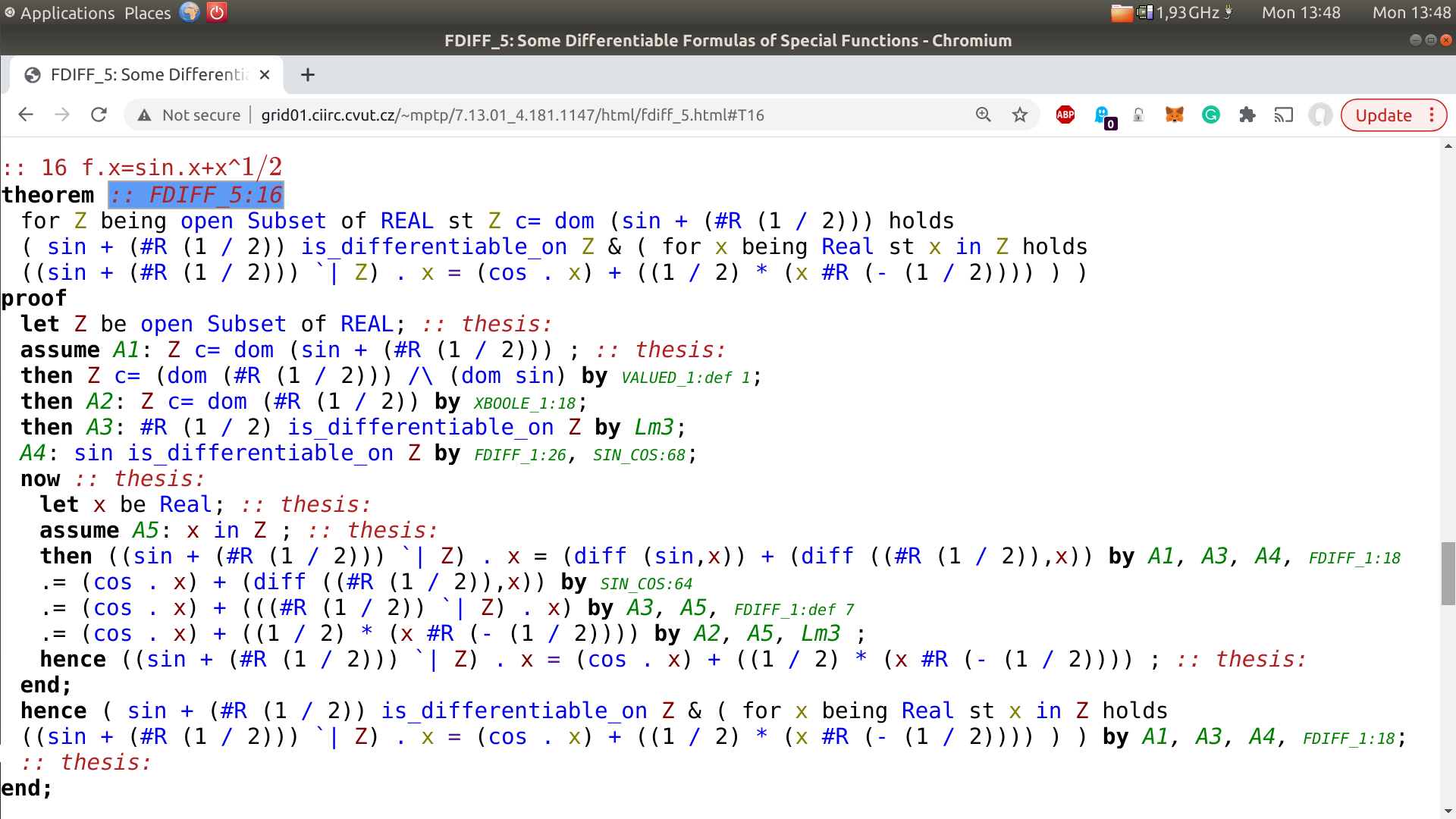
Figure 1: Differentiation – T16_FDIFF_5

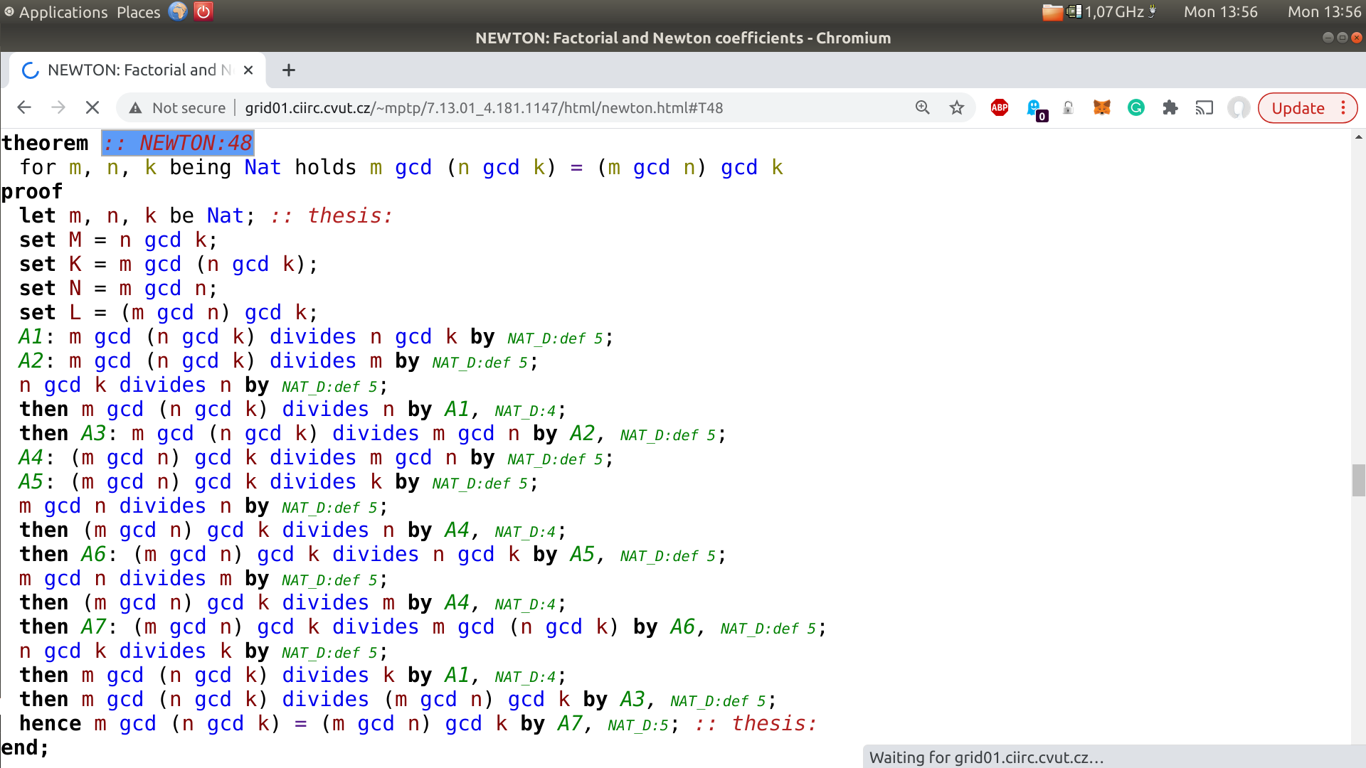
Figure 2: Associativity of gcd by many rewrites – T48_NEWTON

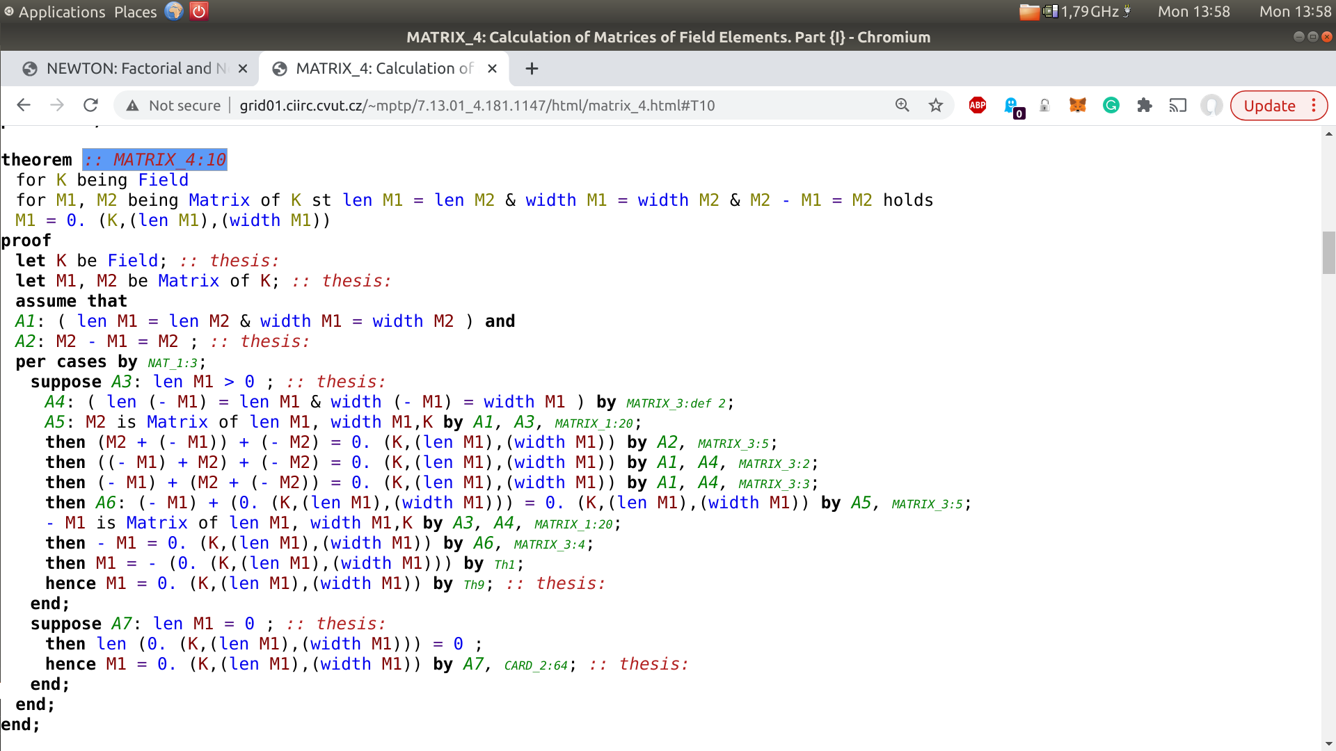
Figure 3: Matrix manipulation – T10_MATRIX_4

References

- [1] Behzad Akbarpour and Lawrence C. Paulson. MetiTarski: An automatic theorem prover for real-valued special functions. J. Autom. Reasoning, 44(3):175–205, 2010.
- [2] Jesse Alama, Tom Heskes, Daniel Kühlwein, Evgeni Tsivtsivadze, and Josef Urban. Premise selection for mathematics by corpus analysis and kernel methods. J. Autom. Reasoning, 52(2):191–213, 2014.
- [3] James C. Bezdek, Robert Ehrlich, and William Full. Fcm: The fuzzy c-means clustering algorithm. Computers & Geosciences, 10(2):191–203, 1984.
- [4] Jasmin Christian Blanchette, Cezary Kaliszyk, Lawrence C. Paulson, and Josef Urban. Hammering towards QED. J. Formalized Reasoning, 9(1):101–148, 2016.
- [5] Vincent D Blondel, Jean-Loup Guillaume, Renaud Lambiotte, and Etienne Lefebvre. Fast unfolding of communities in large networks. Journal of statistical mechanics: theory and experiment, 2008(10):P10008, 2008.
- [6] Karel Chvalovský, Jan Jakubův, Martin Suda, and Josef Urban. ENIGMA-NG: efficient neural and gradient-boosted inference guidance for E. In Pascal Fontaine, editor, Automated Deduction - CADE 27 - 27th International Conference on Automated Deduction, Natal, Brazil, August 27-30, 2019, Proceedings, volume 11716 of Lecture Notes in Computer Science, pages 197–215. Springer, 2019.
- [7] Madson Luiz Dantas Dias. fuzzy-c-means: An implementation of fuzzy -means clustering algorithm., 2019.
- [8] John Ellson, Emden R. Gansner, Eleftherios Koutsofios, Stephen C. North, and Gordon Woodhull. Graphviz and dynagraph - static and dynamic graph drawing tools. In Michael Jünger and Petra Mutzel, editors, Graph Drawing Software, pages 127–148. Springer, 2004.
- [9] Thibault Gauthier, Cezary Kaliszyk, and Josef Urban. TacticToe: Learning to reason with HOL4 tactics. In Thomas Eiter and David Sands, editors, LPAR-21, 21st International Conference on Logic for Programming, Artificial Intelligence and Reasoning, Maun, Botswana, May 7-12, 2017, volume 46 of EPiC Series in Computing, pages 125–143. EasyChair, 2017.
- [10] John C Gittins. Bandit processes and dynamic allocation indices. J. the Royal Statistical Society. Series B (Methodological), pages 148–177, 1979.
- [11] Georg Gottlob, Geoff Sutcliffe, and Andrei Voronkov, editors. Global Conference on Artificial Intelligence, GCAI 2015, Tbilisi, Georgia, October 16-19, 2015, volume 36 of EPiC Series in Computing. EasyChair, 2015.
- [12] Jan Jakubův, Karel Chvalovský, Miroslav Olšák, Bartosz Piotrowski, Martin Suda, and Josef Urban. ENIGMA anonymous: Symbol-independent inference guiding machine (system description). In Nicolas Peltier and Viorica Sofronie-Stokkermans, editors, Automated Reasoning - 10th International Joint Conference, IJCAR 2020, Paris, France, July 1-4, 2020, Proceedings, Part II, volume 12167 of Lecture Notes in Computer Science, pages 448–463. Springer, 2020.
- [13] Jan Jakubův and Josef Urban. Extending E prover with similarity based clause selection strategies. In Michael Kohlhase, Moa Johansson, Bruce R. Miller, Leonardo de Moura, and Frank Wm. Tompa, editors, Intelligent Computer Mathematics - 9th International Conference, CICM 2016, Bialystok, Poland, July 25-29, 2016, Proceedings, volume 9791 of Lecture Notes in Computer Science, pages 151–156. Springer, 2016.
- [14] Jan Jakubův and Josef Urban. ENIGMA: efficient learning-based inference guiding machine. In Herman Geuvers, Matthew England, Osman Hasan, Florian Rabe, and Olaf Teschke, editors, Intelligent Computer Mathematics - 10th International Conference, CICM 2017, Edinburgh, UK, July 17-21, 2017, Proceedings, volume 10383 of Lecture Notes in Computer Science, pages 292–302. Springer, 2017.
- [15] Jan Jakubův and Josef Urban. Hierarchical invention of theorem proving strategies. AI Commun., 31(3):237–250, 2018.
- [16] Jan Jakubův and Josef Urban. Hammering Mizar by learning clause guidance. In John Harrison, John O’Leary, and Andrew Tolmach, editors, 10th International Conference on Interactive Theorem Proving, ITP 2019, September 9-12, 2019, Portland, OR, USA, volume 141 of LIPIcs, pages 34:1–34:8. Schloss Dagstuhl - Leibniz-Zentrum für Informatik, 2019.
- [17] Cezary Kaliszyk and Josef Urban. MizAR 40 for Mizar 40. J. Autom. Reasoning, 55(3):245–256, 2015.
- [18] Cezary Kaliszyk, Josef Urban, Henryk Michalewski, and Miroslav Olšák. Reinforcement learning of theorem proving. In Advances in Neural Information Processing Systems 31: Annual Conference on Neural Information Processing Systems 2018, NeurIPS 2018, 3-8 December 2018, Montréal, Canada., pages 8836–8847, 2018.
- [19] Michael K. Kinyon, Robert Veroff, and Petr Vojtechovský. Loops with abelian inner mapping groups: An application of automated deduction. In Maria Paola Bonacina and Mark E. Stickel, editors, Automated Reasoning and Mathematics - Essays in Memory of William W. McCune, volume 7788 of LNCS, pages 151–164. Springer, 2013.
- [20] Laura Kovács and Andrei Voronkov. First-order theorem proving and Vampire. In Natasha Sharygina and Helmut Veith, editors, CAV, volume 8044 of LNCS, pages 1–35. Springer, 2013.
- [21] William McCune. OTTER 2.0. In Mark E. Stickel, editor, 10th International Conference on Automated Deduction, Kaiserslautern, FRG, July 24-27, 1990, Proceedings, volume 449 of Lecture Notes in Computer Science, pages 663–664. Springer, 1990.
- [22] William McCune. Prover9 and Mace4. http://www.cs.unm.edu/~mccune/prover9/, 2005–2010.
- [23] William McCune. Semantic guidance for saturation provers. In Jacques Calmet, Tetsuo Ida, and Dongming Wang, editors, Artificial Intelligence and Symbolic Computation, 8th International Conference, AISC 2006, Beijing, China, September 20-22, 2006, Proceedings, volume 4120 of Lecture Notes in Computer Science, pages 18–24. Springer, 2006.
- [24] W.W. McCune. Otter 3.3 Reference Manual. Technical Report ANL/MSC-TM-263, Argonne National Laboratory, Argonne, USA, 2003.
- [25] Miroslav Olšák, Cezary Kaliszyk, and Josef Urban. Property invariant embedding for automated reasoning. In Giuseppe De Giacomo, Alejandro Catalá, Bistra Dilkina, Michela Milano, Senén Barro, Alberto Bugarín, and Jérôme Lang, editors, ECAI 2020 - 24th European Conference on Artificial Intelligence, 29 August-8 September 2020, Santiago de Compostela, Spain, August 29 - September 8, 2020 - Including 10th Conference on Prestigious Applications of Artificial Intelligence (PAIS 2020), volume 325 of Frontiers in Artificial Intelligence and Applications, pages 1395–1402. IOS Press, 2020.
- [26] Jens Otten and Wolfgang Bibel. leanCoP: lean connection-based theorem proving. J. Symb. Comput., 36(1-2):139–161, 2003.
- [27] Art Quaife. Automated Development of Fundamental Mathematical Theories. Kluwer Academic Publishers, 1992.
- [28] Thomas Raths and Jens Otten. randocop: Randomizing the proof search order in the connection calculus. In Boris Konev, Renate A. Schmidt, and Stephan Schulz, editors, Proceedings of the First International Workshop on Practical Aspects of Automated Reasoning, Sydney, Australia, August 10-11, 2008, volume 373 of CEUR Workshop Proceedings. CEUR-WS.org, 2008.
- [29] John Alan Robinson and Andrei Voronkov, editors. Handbook of Automated Reasoning (in 2 volumes). Elsevier and MIT Press, 2001.
- [30] Simon Schäfer and Stephan Schulz. Breeding theorem proving heuristics with genetic algorithms. In Gottlob et al. [11], pages 263–274.
- [31] Stephan Schulz. E - A Brainiac Theorem Prover. AI Commun., 15(2-3):111–126, 2002.
- [32] Stephan Schulz. System description: E 1.8. In Kenneth L. McMillan, Aart Middeldorp, and Andrei Voronkov, editors, LPAR, volume 8312 of LNCS, pages 735–743. Springer, 2013.
- [33] Josef Urban. MPTP 0.2: Design, implementation, and initial experiments. J. Autom. Reasoning, 37(1-2):21–43, 2006.
- [34] Josef Urban. BliStr: The Blind Strategymaker. In Gottlob et al. [11], pages 312–319.
- [35] Robert Veroff. Using hints to increase the effectiveness of an automated reasoning program: Case studies. J. Autom. Reasoning, 16(3):223–239, 1996.
- [36] Pauli Virtanen, Ralf Gommers, Travis E. Oliphant, Matt Haberland, Tyler Reddy, David Cournapeau, Evgeni Burovski, Pearu Peterson, Warren Weckesser, Jonathan Bright, Stéfan J. van der Walt, Matthew Brett, Joshua Wilson, K. Jarrod Millman, Nikolay Mayorov, Andrew R. J. Nelson, Eric Jones, Robert Kern, Eric Larson, C J Carey, İlhan Polat, Yu Feng, Eric W. Moore, Jake VanderPlas, Denis Laxalde, Josef Perktold, Robert Cimrman, Ian Henriksen, E. A. Quintero, Charles R. Harris, Anne M. Archibald, Antônio H. Ribeiro, Fabian Pedregosa, Paul van Mulbregt, and SciPy 1.0 Contributors. SciPy 1.0: Fundamental Algorithms for Scientific Computing in Python. Nature Methods, 17:261–272, 2020.