Nonuniqueness and nonlinear instability of Gaussons under repulsive harmonic potential

Abstract.

We consider the Schrödinger equation with a nondispersive logarithmic nonlinearity and a repulsive harmonic potential. For a suitable range of the coefficients, there exist two positive stationary solutions, each one generating a continuous family of solitary waves. These solutions are Gaussian, and turn out to be orbitally unstable. We also discuss the notion of ground state in this setting: for any natural definition, the set of ground states is empty.

1. Introduction

We consider the equation

(1.1) $$i{\partial}_{t}u+\frac{1}{2}\Delta u=-\omega^{2}\frac{|x|^{2}}{2}u+\lambda u\ln\left(|u|^{2}\right),\quad x\in{\mathbb{R}}^{d},$$

in the case $\omega>0$ (repulsive harmonic potential) and $\lambda<0$. The logarithmic Schrödinger equation ((1.1) with $\omega=0$) was introduced in [6], and has been considered in various fields of physics since; see e.g. [4, 9, 18, 19, 24, 26, 33] and references therein. A special feature of the logarithmic nonlinearity is that it leads to very special solitary waves, called Gaussons in [6, 7]: if $\lambda<0$, for any $\nu\in{\mathbb{R}}$,

$$e^{i\nu t}e^{\frac{\lambda d-\nu}{2\lambda}}e^{\lambda|x|^{2}}$$

is a solution to (1.1) (with $\omega=0$). These solitary waves are orbitally stable, as proved in [14] (radial case) and [2] (general case). In addition, still in the case $\omega=0$, it is known that for $\lambda<0$, no solution is dispersive ([14, Proposition 4.3]), while for $\lambda>0$, every solution is dispersive, with an enhanced rate compared to the usual rate of the free Schrödinger equation ([12]).

The logarithmic Schrödinger equation in the presence of a confining harmonic potential was considered in physics in [8],

(1.2) $$i{\partial}_{t}u+\frac{1}{2}\Delta u=\omega^{2}\frac{|x|^{2}}{2}u+\lambda u\ln\left(|u|^{2}\right),\quad x\in{\mathbb{R}}^{d}.$$

In the case $\lambda<0$ ([3]) as well as in the case $\lambda>0$ ([11]), generalized Gaussons exist, and are orbitally stable, in the sense introduced in [16] (see Definition 1.1 below for the definition in the case of (1.1), the notion being the same for (1.2)).

The case of an inverted, or repulsive harmonic potential as in (1.1), does not seem to correspond to a realistic model, but constitutes an interesting mathematical toy. The potential $V(x)=-\omega^{2}\frac{|x|^{2}}{2}$ is unbounded from below, and goes to $-\infty$ as fast as possible in order to guarantee that the Hamiltonian $-\frac{1}{2}\Delta+V(x)$ is essentially self-adjoint on $C_{0}^{\infty}({\mathbb{R}}^{d})$; see [17, 28]. In the linear case $\lambda=0$, classical trajectories go to infinity exponentially fast in time, the solution disperses exponentially in time, and the Sobolev norms grow exponentially in time (see e.g. [10]). Because of that, there are no long range effects (scattering theory) when a power-like nonlinearity is added ([10]), and at least in the case of an $L^{2}$-critical focusing nonlinearity,

$$i{\partial}_{t}u+\frac{1}{2}\Delta u=-\omega^{2}\frac{|x|^{2}}{2}u-|u|^{4/d}u,\quad x\in{\mathbb{R}}^{d},$$

there exists no nontrivial solitary wave $u(t,x)=e^{i\nu t}\phi(x)$ with $\phi\in L^{2}({\mathbb{R}}^{d})$ [22, 23].

In the case of (1.1), the mass and the energy are formally independent of time: they are given by

(1.3) $$M(u) =\|u\|_{L^{2}({\mathbb{R}}^{d})}^{2},$$

$$E(u) =\frac{1}{2}\|\nabla u\|_{L^{2}({\mathbb{R}}^{d})}^{2}-\frac{\omega^{2}}{2}\|xu\|_{L^{2}}^{2}+\lambda\int_{{\mathbb{R}}^{d}}|u|^{2}\left(\ln|u|^{2}-1\right)dx.$$

The energy has no definite sign, for two reasons: the repulsive harmonic potential has a negative contribution in $E$, and the logarithmic nonlinearity induces a potential energy with indefinite sign (entropy). Introduce the space $\Sigma$ defined by

$$\Sigma=H^{1}\cap\mathcal{F}(H^{1})=\left\{f\in H^{1}({\mathbb{R}}^{d}),\quad x\mapsto|x|f(x)\in L^{2}({\mathbb{R}}^{d})\right\},$$

and equipped with the norm

$$\|f\|_{\Sigma}^{2} =\|f\|_{L^{2}({\mathbb{R}}^{d})}^{2}+\|\nabla f\|_{L^{2}({\mathbb{R}}^{d})}^{2}+\int_{{\mathbb{R}}^{d}}|x|^{2}|f(x)|^{2}dx$$

$$=\|f\|_{L^{2}({\mathbb{R}}^{d})}^{2}+\left\langle\left(-\Delta+|x|^{2}\right)f,f\right\rangle.$$

It is proved in [11, Proposition 1.3] that for $\lambda\in{\mathbb{R}}$ and any $u_{0}\in\Sigma$, there exists a unique solution $u\in L^{\infty}_{\rm loc}({\mathbb{R}};\Sigma)\cap C({\mathbb{R}};L^{2}({\mathbb{R}}^{d}))$ to (1.1), such that $u_{\mid t=0}=u_{0}$. In addition, the mass $M$ and the energy $E$ are independent of time. In [11], it is proved in addition that in the case $\lambda>0$, every solution to (1.1) disperses exponentially fast: in particular, there is no solitary wave in this case.

The situation is different in the case $\lambda<0$, and leads to features which appear to be quite unique, in the context of the logarithmic Schrödinger equation (with potential), and more generally of nonlinear Schrödinger equations. In [32], it was proven that (1.1) admits at least one positive bound state, under some conditions on the coefficients, recalled below. Under suitable assumptions regarding the parameters $\lambda$ and $\omega$, we exhibit two positive stationary solutions.

Due to the presence of the potential, (1.1) is not invariant by translation in space, hence the definition below (as in [3]):

Definition 1.1.

A standing wave $u(t,x)=\phi(x)e^{i\nu t}$ solution to (1.1) is orbitally stable in the energy space if for any $\varepsilon>0$, there exists $\eta>0$ such that if $u_{0}\in\Sigma$ satisfies $\|u_{0}-\phi\|_{\Sigma}<\eta$, then the solution $u$ to (1.1) exists for all $t\in{\mathbb{R}}$, and

$$\sup_{t\in{\mathbb{R}}}\inf_{\theta\in{\mathbb{R}}}\|u(t)-e^{i\theta}\phi\|_{\Sigma}<\varepsilon.$$

Otherwise, the standing wave is said to be unstable.

The main result of this paper is the following:

Theorem 1.2.

Let $-\lambda>\omega>0$. Then (1.1) possesses two positive stationary solutions, which are Gaussons,

$$\phi_{k_{\pm}}(x)=e^{-\frac{dk_{\pm}}{4\lambda}}e^{-k_{\pm}|x|^{2}/2},\quad\text{where}\quad k_{\pm}=-\lambda\pm\sqrt{\lambda^{2}-\omega^{2}}.$$

Each stationary solution generates a continuous family of solitary waves,

$$u_{\pm,\nu}(t,x)=\phi_{k_{\pm},\nu}(x)e^{i\nu t},\quad\phi_{k_{\pm},\nu}(x)=e^{-\frac{\nu}{2\lambda}}\phi_{k_{\pm}}(x),\quad\nu\in{\mathbb{R}}.$$

Every such solitary wave is unstable in the sense of Definition 1.1.
In the limiting case $-\lambda=\omega>0$, $\phi_{k_{-}}=\phi_{k_{+}}=\phi_{\omega}=e^{d/4}e^{-\omega|x|^{2}/2}$ also generates a continuous family of solitary waves,

$$u_{\omega,\nu}(t,x)=\phi_{\omega,\nu}(x)e^{i\nu t},\quad\phi_{\omega,\nu}(x)=e^{\frac{\nu}{2\omega}}\phi_{\omega}(x),\quad\nu\in{\mathbb{R}},$$

and every such solitary wave is unstable in the sense of Definition 1.1.

We note that $\phi_{k_{-}}$ and $\phi_{k_{+}}$ are two positive solutions to the stationary equation

(1.4) $$-\frac{1}{2}\Delta\phi-\omega^{2}\frac{|x|^{2}}{2}\phi+\lambda\phi\ln\left(|\phi|^{2}\right)=0.$$

As evoked above, it is shown in [32] that (1.1) has at least one positive solution, under suitable assumptions on the coefficients of the equation. More precisely, in [32], a semiclassical parameter $\varepsilon$ is present,

$$-\varepsilon^{2}\Delta u-|x|^{2}u=u\ln|u|^{2}.$$

A stationary, positive solution exists for sufficiently small values of the semiclassical parameter $\varepsilon$: a rescaling argument shows that this corresponds to (1.4) the case $\lambda=-2$, with $\omega=\varepsilon$: for $\varepsilon$ small, we indeed have $-\lambda>\omega>0$. In [1], it is shown that for the logarithmic Schrödinger equation with a potential admitting a global minimum reached in $\ell\geqslant 2$ points sufficiently far one from another, there exist at least $\ell$ positive stationary solutions, providing a situation where nonuniqueness holds, which is quite different from ours.

Linearizing (1.1) around $\phi_{k}$, for $k=k_{-}$ or $k_{+}$, leads to:

$$i{\partial}_{t}u+\frac{1}{2}\Delta u=-\omega^{2}\frac{|x|^{2}}{2}u-\frac{dk}{2}u-\lambda k|x|^{2}u=k^{2}\frac{|x|^{2}}{2}u-\frac{dk}{2}u.$$

The underlying Hamiltonian is the (shifted) harmonic oscillator,

$$H_{k}=-\frac{1}{2}\Delta+k^{2}\frac{|x|^{2}}{2}-\frac{dk}{2},$$

whose point spectrum is $k{\mathbb{N}}$. This implies linear and spectral stability of the stationary states $\phi_{k_{\pm}}$, like e.g. for the Gausson in the case of the logarithmic KdV equation [13, 20, 27]. From this perspective, the nonlinear instability stated in Theorem 1.2 can appear surprising. We actually show several possible mechanisms leading to instability.

Ground states are often characterized as the unique positive solution to an elliptic equation (typically when the nonlinearity is homogeneous, but not only, see e.g. [21, 25]): we discuss more into details the notion of ground state in Section 4, and show that neither $\phi_{k_{-}}$ nor $\phi_{k_{+}}$ can be considered as a ground state according to standard definitions. Note that the underlying operator $-\Delta-\omega^{2}|x|^{2}$ is not elliptic, since its symbol is $|\xi|^{2}-\omega^{2}|x|^{2}$. In particular, we do not obtain a variational characterization of the Gaussons in the present case, unlike in the case without potential [2], or with a confining harmonic potential [3, 11]. This is consistent with the fact that these solutions are unstable. Note however that in view of the global existence result [11, Proposition 1.3], the instability mechanism is not related to finite time blow-up.

The rest of this paper is organized as follows. In Section 2, we show some special invariances and discuss more into details special Gaussian solutions to (1.1). In Section 3, we complete the proof of Theorem 1.2, by showing the instability of $\phi_{k_{-}}$ and $\phi_{k_{+}}$; several causes of instability are exhibited. Finally in Section 4, we discuss the notion of ground state associated to (1.1), and show that it should be considered that (1.1) possesses no ground state.

2. Special solutions and invariances

2.1. Some invariances

(1.1) is invariant with respect to translation in time, but not with respect to translation in space, due to the potential. It is gauge invariant: if $u$ is a solution, then so is $e^{i\theta}u$ for any constant $\theta\in{\mathbb{R}}$.

Size effect.

The following invariance is a feature of the logarithmic nonlinearity: If $u$ solves (1.1), then for all $c\in{\mathbb{C}}$, so does

(2.1) $$u_{c}(t,x):=c\,u(t,x)e^{-it\lambda\ln|c|^{2}}.$$

Typically, if we find a stationary solution, then the above transform generates a continuum of solitary waves, indexed by $c\in(0,\infty)$, or equivalently by

$$\nu=-\lambda\ln\left(c^{2}\right)\in{\mathbb{R}}.$$

Note that the size of these solitary waves is arbitrary, as $c$ ranges $(0,\infty)$.

Galilean invariance.

Due to the repulsive harmonic potential, the Galilean invariance reads are follows: If $u(t,x)$ solves (1.1), then for any $v\in{\mathbb{R}}^{d}$, so does

(2.2) $$u\left(t,x-v\frac{\sinh(\omega t)}{\omega}\right)\exp\left(i\cosh(\omega t)v\cdot x-\frac{i|v|^{2}}{4\omega}\sinh(2\omega t)\right).$$

At $t=0$, the above transform is just a multiplication by $e^{iv\cdot x}$.

Space translation.

The absence of invariance with respect to translation in space can be specified as follows: If $u$ solves (1.1), then for any $x_{0}\in{\mathbb{R}}^{d}$, so does

(2.3) $$u\left(t,x-x_{0}\cosh(\omega t)\right)\exp\left(i\omega\sinh(\omega t)x_{0}\cdot x-\frac{i\omega|x_{0}|^{2}}{4}\sinh(2\omega t)\right).$$

At $t=0$, the above transform corresponds to a shift in space.

Tensorization.

The logarithmic nonlinearity was introduced in [6] to satisfy the following tensorization property: as the external potential decouples space variables,

$$-\omega^{2}\frac{|x|^{2}}{2}=-\frac{\omega^{2}}{2}\sum_{j=1}^{d}x_{j}^{2},$$

if the initial datum is a tensor product,

$$u_{0}(x)=\prod_{j=1}^{d}u_{0j}(x_{j}),$$

then the solution to (1.1) is given by

$$u(t,x)=\prod_{j=1}^{d}u_{j}(t,x_{j}),$$

where each $u_{j}$ solves a one-dimensional equation,

$$i{\partial}_{t}u_{j}+\frac{1}{2}{\partial}_{x_{j}}^{2}u_{j}=-\omega^{2}\frac{x_{j}^{2}}{2}u_{j}+\lambda\ln\left(|u_{j}|^{2}\right)u_{j},\quad u_{j\mid t=0}=u_{0j}.$$

2.2. Gaussons

As announced in the introduction, for $-\lambda>\omega>0$, the stationary Gaussons are given by

$$\phi_{k}(x)=e^{-\frac{dk}{4\lambda}}e^{-k|x|^{2}/2},$$

where $k$ is either of the solutions to

(2.4) $$k^{2}+2\lambda k+\omega^{2}=0,\text{ i.e. }k_{\pm}=-\lambda\pm\sqrt{\lambda^{2}-\omega^{2}}.$$

If $-\lambda=\omega>0$, then $k_{-}=k_{+}=\omega$, and we will see in the next subsection that when $\omega>-\lambda>0$, there exists no Gausson. We compute

$$\|\phi_{k}\|_{L^{2}({\mathbb{R}}^{d})}^{2}=e^{-\frac{dk}{2\lambda}}\left(\frac{\pi}{k}\right)^{d/2}.$$

We note that as $\omega\to 0$ with $\lambda<0$ fixed, $k_{-}\to 0$, $k_{+}\to-2\lambda$, hence

$$\|\phi_{k_{-}}\|_{L^{2}({\mathbb{R}}^{d})}^{2}\to\infty,\quad\text{whereas}\quad\|\phi_{k_{+}}\|_{L^{2}({\mathbb{R}}^{d})}^{2}\to e^{d}\left(\frac{\pi}{-2\lambda}\right)^{d/2}.$$

We have more generally

Lemma 2.1.

Let $-\lambda>\omega>0$. We have

$$\|\phi_{k_{-}}\|_{L^{2}({\mathbb{R}}^{d})}>\|\phi_{k_{+}}\|_{L^{2}({\mathbb{R}}^{d})}.$$

Proof.

It suffices to prove that

$$\frac{e^{-k_{-}/\lambda}}{k_{-}}>\frac{e^{-k_{+}/\lambda}}{k_{+}} \Longleftrightarrow e^{(k_{+}-k_{-})/\lambda}>\frac{k_{-}}{k_{+}}$$

$$\Longleftrightarrow e^{2\sqrt{\lambda^{2}-\omega^{2}}/\lambda}>\frac{-\lambda-\sqrt{\lambda^{2}-\omega^{2}}}{-\lambda+\sqrt{\lambda^{2}-\omega^{2}}}.$$

We view the above inequality as depending on the unknown $\omega\in(0,-\lambda)$, and change the unknown as $\theta=\sqrt{\lambda^{2}-\omega^{2}}/|\lambda|\in(0,1)$, so the above inequality becomes

$$e^{-2\theta}>\frac{1-\theta}{1+\theta}\Longleftrightarrow 1+\theta>(1-\theta)e^{2\theta}.$$

The map $f(\theta)=1+\theta-(1-\theta)e^{2\theta}$, defined for $\theta\in(0,1)$, satisfies

$$f^{\prime\prime}(\theta)=4e^{2\theta}-4(1-\theta)e^{2\theta}>0,\text{ hence }f^{\prime}(\theta)=1+e^{2\theta}-2(1-\theta)e^{2\theta}>0,$$

and $f(\theta)>0$ for all $0<\theta<1$. ∎

In view of (2.1), with $\nu=-\lambda\ln(c^{2})$, $c>0$, we have a continuum of standing waves:

$$u_{\pm,\nu}(t,x)=\phi_{k_{\pm},\nu}(x)e^{i\nu t},\quad\phi_{k_{\pm},\nu}(x)=e^{-\frac{\nu}{2\lambda}}\phi_{k_{\pm}}(x),\quad\nu\in{\mathbb{R}}.$$

Therefore, to understand the dynamical properties of $u_{\pm,\nu}$ (orbital stability or instability), it is enough to consider the stationary solutions $\phi_{k_{\pm}}$.

2.3. Gaussian solutions

By Gaussian solutions, we mean solutions which are Gaussian in the space variable, with time-dependent coefficients. We adapt the computations presented in [12] in the case $\omega=0$. Suppose $d=1$ (for $d\geqslant 2$, we may invoke the above tensorization property). We seek $u(t,x)=b(t)e^{-a(t)x^{2}/2}$ (in particular $u_{0}$ is Gaussian). We find:

$$i\dot{b}=\frac{1}{2}ab+\lambda b\ln|b|^{2};\quad i\dot{a}=a^{2}+2\lambda\operatorname{Re}a+\omega^{2}.$$

The function $b$ is given explicitly in terms of $a$ and its initial value $b_{0}$,

$$b(t)=b_{0}\exp\left(-i\lambda t\ln\left(|b_{0}|^{2}\right)-\frac{i}{2}A(t)-i\lambda\operatorname{Im}\int_{0}^{t}A(s)ds\right),$$

where we have denoted $\displaystyle A(t)=\int_{0}^{t}a(s)ds$. We may write $a$ under the form

(2.5) $$a=\frac{1}{\tau^{2}}-i\frac{\dot{\tau}}{\tau},\quad\tau\in\mathbb{R},$$

and the equation for $a$ leads to

(2.6) $$\ddot{\tau}=\frac{2\lambda}{\tau}+\frac{1}{\tau^{3}}+\omega^{2}\tau.$$

We note that the form (2.5) implies that $b(t)$ can be written as

(2.7) $$b(t)=b_{0}e^{i\theta(t)}\sqrt{\frac{\tau(0)}{\tau(t)}},\quad\theta(t)\in{\mathbb{R}}.$$

Multiplying (2.6) by $\dot{\tau}$ and integrating, we get

(2.8) $$(\dot{\tau})^{2}=C_{0}+4\lambda\ln|\tau|-\frac{1}{\tau^{2}}+\omega^{2}\tau^{2},$$

where $C_{0}=\dot{\tau}(0)^{2}-4\lambda\ln|\tau(0)|+\frac{1}{\tau(0)^{2}}-\omega^{2}\tau(0)^{2}$ is related to the initial data. Noticing that $F(q)=C_{0}+4\lambda\ln q-\frac{1}{q^{2}}+\omega^{2}q^{2}\to-\infty$ when $q\to 0$, this readily shows that $\tau$ remains bounded away from zero, and thus may be supposed positive in view of (2.5):

$$\exists\delta>0,\quad\tau(t)\geqslant\delta,\quad\forall t\geqslant 0.$$

Proposition 2.2.

Let $d=1$, $\lambda<0<\omega$.
$1.$ If $-\lambda>\omega>0$, then (2.6) has exactly two stationary solutions, $\tau_{\mp}=1/\sqrt{k_{\pm}}$. The other solutions are either periodic, or unbounded, corresponding to time-periodic and dispersive Gaussian solutions to (1.1), respectively.
$2.$ If $-\lambda=\omega>0$, then (2.6) has exactly one stationary solution, $\tau_{0}=1/\sqrt{\omega}$. All the other solutions are unbounded. In other words, any Gaussian solution to (1.1) which is not of the form

$$e^{(2\nu+\omega)/(4\omega)}e^{i\nu t}e^{-\omega x^{2}/2},\quad\nu\in{\mathbb{R}},$$

is dispersive.
$3.$ If $\omega>-\lambda>0$, then every solution to (2.6) is unbounded. More precisely,

$$e^{\omega t}\lesssim\tau(t)\lesssim e^{\omega t},\quad t\geqslant 0,$$

and every Gaussian solution to (1.1) disperses exponentially fast.

Proof.

We remark that the righthand side of (2.6) can be rewritten as

$$\ddot{\tau}=P\left(\frac{1}{\tau^{2}}\right)\tau,\quad P(X)=X^{2}+2\lambda X+\omega^{2}.$$

When $-\lambda>\omega>0$, $P$ has exactly two roots, $k_{-}$ and $k_{+}$, so

$$\ddot{\tau}=\left(\frac{1}{\tau^{2}}-k_{-}\right)\left(\frac{1}{\tau^{2}}-k_{+}\right)\tau.$$

According to the initial data for $\tau$, the value of the constant $C_{0}$ in (2.8) varies, leading to bounded trajectories, in which case $\tau$ is periodic, or to unbounded trajectories, in which case $\tau(t)\to\infty$ as $t$ goes to infinity. This is illustrated by Figure 1, displaying the phase portrait for the equation (2.6) with $\omega=1$ and $\lambda=-2$, where we find

$$\tau_{-}=\frac{1}{\sqrt{2+\sqrt{3}}}\approx 0.518,\quad\tau_{+}=\frac{1}{\sqrt{2-\sqrt{3}}}\approx 1.932.$$

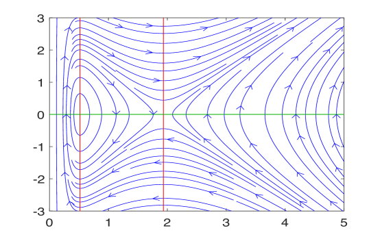
Figure 1. Phase portraits for the ODE (2.6) with $\omega=1$ and $\lambda=-2$.

When $-\lambda=\omega>0$, $P$ has exactly one double root $\omega$, and

$$\ddot{\tau}=\left(\frac{1}{\tau^{2}}-\omega\right)^{2}\tau.$$

If $\tau$ is not constant (equal to $1/\sqrt{\omega}$), then $\tau$ is strictly convex. If $\tau(t_{0})=1/\sqrt{\omega}$ for some $t_{0}\geqslant 0$, then $\dot{\tau}(t_{0})\not=0$, for otherwise $\tau$ would be constant, by uniqueness for (2.6): $\tau$ can’t remain close to $1/\sqrt{\omega}$, and assuming that $\tau$ is bounded leads to a contradiction. As $\tau$ is positive and convex, $\tau(t)$ goes to infinity as $t\to\infty$. This is illustrated in Figure 2.

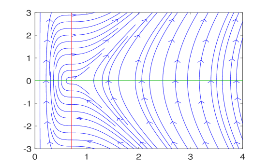
Figure 2. Phase portraits for the ODE (2.6) with $\omega=2$ and $\lambda=-2$.

When $\omega>-\lambda>0$, $P$ is uniformly bounded from below on ${\mathbb{R}}$, $P(X)\geqslant\delta>0$. If $\tau$ was bounded, (2.6) would yield $\ddot{\tau}\gtrsim 1$, since $\tau$ is bounded away from zero, hence a contradiction. As $\tau$ is convex, $\tau(t)$ goes to infinity as $t\to\infty$, see Figure 3.

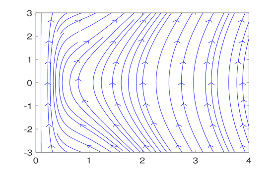
Figure 3. Phase portraits for the ODE (2.6) with $\omega=2$ and $\lambda=-1$.

As a consequence, for any $\varepsilon>0$, picking $T$ sufficiently large,

$$\ddot{\tau}(t)\geqslant\omega^{2}\tau(t)-\varepsilon,\quad\forall t\geqslant T.$$

The solution to

$$\ddot{\theta}(t)=\omega^{2}\theta(t)-\varepsilon,\quad\theta(T)=\tau(T),\quad\dot{\theta}(T)=\dot{\tau}(T),$$

is given by

$$\theta(t)=\tau(T)\cosh\left(\omega(t-T)\right)+\dot{\tau}(T)\frac{\sinh\left(\omega(t-T)\right)}{\omega}-\frac{2\varepsilon}{\omega^{2}}\sinh^{2}\left(\frac{\omega}{2}(t-T)\right).$$

As $\tau(T)$ and $\dot{\tau}(T)$ go to infinity as $T\to\infty$, we infer that $\tau(t)\gtrsim e^{\omega t}$. The converse estimate is a direct consequence of (2.8), again because for $t$ sufficiently large, $\ln\tau(t)>0$, and $\lambda<0$. ∎

3. Orbital instability

The instability result that we prove is slightly stronger than instability in the sense of Definition 1.1:

Lemma 3.1.

Let $\nu\in{\mathbb{R}}$.
$1.$ Suppose $-\lambda>\omega>0$. The solitary waves $\phi_{k_{-},\nu}(x)e^{i\nu t}$ and $\phi_{k_{+},\nu}(x)e^{i\nu t}$ are unstable. More precisely, for any $\eta>0$, there exists $u_{0}\in\Sigma$ such that

$$\|u_{0}-\phi_{k_{+},\nu}\|_{\Sigma}<\eta,$$

and the solution to (1.1) such that $u_{\mid t=0}=u_{0}$ satisfies

$$\sup_{t\geqslant 0}\inf_{\theta\in{\mathbb{R}}}\left\|u(t)-e^{i\theta}\phi_{k_{+},\nu}\right\|_{L^{2}({\mathbb{R}}^{d})}\geqslant\frac{1}{2}\|\phi_{k_{+},\nu}\|_{L^{2}({\mathbb{R}}^{d})}.$$

The same holds when $k_{+}$ is replaced by $k_{-}$.
$2.$ Suppose $-\lambda=\omega>0$. The solitary wave $\phi_{\omega,\nu}(x)e^{i\nu t}$ is unstable in the same sense as above.

Proof.

We present the argument for $\phi_{k_{+}}$, to shorten notations: considering $\phi_{k_{\pm},\nu}$ for $\nu\in{\mathbb{R}}$ goes along the same lines, and the argument includes the limiting case $-\lambda=\omega>0$. For all $\eta>0$, then exists $\delta>0$ such that for $|x_{0}|<\delta$,

$$\|u_{0}-\phi_{k_{+}}\|_{\Sigma}<\eta,\quad u_{0}(x)=\phi_{k_{+}}(x-x_{0}).$$

In view of (2.3), the solution to (1.1) with initial datum $u_{0}$ is given by

$$u(t,x)=\phi_{k_{+}}\left(x-x_{0}\cosh(\omega t)\right)e^{i\omega\sinh(\omega t)x_{0}\cdot x-\frac{i\omega|x_{0}|^{2}}{4}\sinh(2\omega t)}.$$

Therefore, for any $t>0$,

$$\inf_{\theta\in{\mathbb{R}}}\|u(t)-e^{i\theta}\phi_{k_{+}}\|^{2}_{L^{2}({\mathbb{R}}^{d})}\geqslant\int_{{\mathbb{R}}^{d}}\left|\phi_{k_{+}}\left(x-x_{0}\cosh(\omega t)\right)-\phi_{k_{+}}(x)\right|^{2}dx.$$

Indeed, denote $u(t,x)=\phi_{k_{+}}\left(x-x_{0}\cosh(\omega t)\right)e^{i\alpha(x_{0},x,t)}$ with $\alpha(x_{0},x,t)\in{\mathbb{R}}$ given by the above formula. Then

$$\|u(t)-e^{i\theta}\phi_{k_{+}}\|^{2}_{L^{2}({\mathbb{R}}^{d})}=\|\phi_{k_{+}}\left(x-x_{0}\cosh(\omega t)\right)-e^{i(\theta-\alpha(x_{0},x,t))}\phi_{k_{+}}\|^{2}_{L^{2}({\mathbb{R}}^{d})}$$

$$\quad=2\|\phi_{k_{+}}\|^{2}_{L^{2}({\mathbb{R}}^{d})}-2\int_{{\mathbb{R}}^{d}}\cos(\theta-\alpha(x_{0},x,t))\phi_{k_{+}}\left(x-x_{0}\cosh(\omega t)\right)\phi_{k_{+}}(x)dx,$$

which implies

$$\quad\inf_{\theta\in{\mathbb{R}}}\|u(t)-e^{i\theta}\phi_{k_{+}}\|^{2}_{L^{2}({\mathbb{R}}^{d})}$$

$$=2\|\phi_{k_{+}}\|^{2}_{L^{2}({\mathbb{R}}^{d})}-2\sup_{\theta\in{\mathbb{R}}}\int_{{\mathbb{R}}^{d}}\cos(\theta-\alpha(x_{0},x,t))\phi_{k_{+}}\left(x-x_{0}\cosh(\omega t)\right)\phi_{k_{+}}(x)dx$$

$$\geqslant 2\|\phi_{k_{+}}\|^{2}_{L^{2}({\mathbb{R}}^{d})}-2\int_{{\mathbb{R}}^{d}}\phi_{k_{+}}\left(x-x_{0}\cosh(\omega t)\right)\phi_{k_{+}}(x)dx$$

$$=\left\|\phi_{k_{+}}\left(x-x_{0}\cosh(\omega t)\right)-\phi_{k_{+}}(x)\right\|_{L^{2}({\mathbb{R}}^{d})}^{2}.$$

It becomes obvious that picking $t$ sufficiently large (in terms of $\eta$) leads to

$$\inf_{\theta\in{\mathbb{R}}}\|u(t)-e^{i\theta}\phi_{k_{+}}\|^{2}_{L^{2}({\mathbb{R}}^{d})}\geqslant\frac{1}{2}\|\phi_{k_{+}}\|_{L^{2}({\mathbb{R}}^{d})}^{2}.$$

This rules out orbital stability, even in the $L^{2}$-norm, for initial data close to $\phi_{k_{+}}$ in the $\Sigma$-topology. ∎

Remark 3.2.

We can adapt the above proof by using the Galilean invariance (2.2), and consider instead

$$u_{0}(x)=\phi_{k_{+}}(x)e^{iv\cdot x},\quad|v|\ll 1.$$

Remark 3.3.

It is clear from the argument that $u_{0}$ is close to $\phi_{k_{+}}$ in $\Sigma$, but also in stronger norms, while orbital stability is ruled out by measuring only the $L^{2}$-norm.

The above arguments do not rule out orbital stability when the initial datum are restricted to be radially symmetric. In [14], this restriction was considered essentially to obtain compactness properties (the embedding of $H^{1}_{\rm rad}({\mathbb{R}}^{d})$ into $L^{p}({\mathbb{R}}^{d})$ for $2\leqslant p<\frac{2}{(d-2)_{+}}$ is compact). Note that $\Sigma$ is compactly embedded into $L^{p}({\mathbb{R}}^{d})$ for $2\leqslant p<\frac{2}{(d-2)_{+}}$. The lemma below shows instability for $\phi_{k_{-}}$ even at the radial level.

Lemma 3.4.

Let $\nu\in{\mathbb{R}}$.
$1.$ Suppose $-\lambda>\omega>0$. The solitary wave $\phi_{k_{-},\nu}(x)e^{i\nu t}$ is unstable even if we restrict Definition 1.1 to radial solutions.
$2.$ The same holds for $\phi_{\omega,\nu}(x)e^{i\nu t}$ in the case $-\lambda=\omega>0$.

Proof.

Assume $-\lambda>\omega>0$. We show that $u_{k_{-},\nu}$ is unstable even as a Gaussian solution centered at the origin, by linearizing (2.6) about $\tau_{-}=1/\sqrt{k_{-}}$: we compute the linearization as

$$\ddot{h}=\omega^{2}h-2\lambda k_{-}h-3k_{-}^{2}h=\Omega_{\rm eff}h,$$

where

$$\Omega_{\rm eff}=\omega^{2}-2\lambda k_{-}-3k_{-}^{2}=-4k_{-}^{2}-4\lambda k_{-}=-4k_{-}(k_{-}+\lambda).$$

Since $k_{-}+\lambda<0$, the linearized operator is such that $\Omega_{\rm eff}>0$, so $h$ grows exponentially. Of course linearizing makes sense only for sufficiently small $h$, but this is enough to contradict the definition of orbital stability. Indeed, there exists $\delta>0$ such that as long as $|h(t)|\leqslant\delta$, we can write the solution $\tau$ to (2.6) with $\tau(0)=\tau_{-}+h(0)$ and $\dot{\tau}(0)=0$ as

$$\tau(t)=\tau_{-}+h(t)+r(t),\quad\text{with}\quad|r(t)|\leqslant\frac{|h(t)|}{2}.$$

For $0<\varepsilon<\delta$, let $h$ solve

$$\ddot{h}=\Omega_{\rm eff}h,\quad h(0)=\varepsilon,\quad\dot{h}(0)=0.$$

As $h(t)=\varepsilon\cosh(t\sqrt{\Omega_{\rm eff}})$ grows exponentially, there exists $t_{0}>0$ such that $h(t_{0})=\delta$, and the triangle inequality yields

$$|\tau(t_{0})-\tau_{-}|\geqslant\frac{\delta}{2}.$$

Now if $u$ denotes the Gaussian solution associated with $\tau$, we see that for all $\eta>0$, picking $\varepsilon>0$ sufficiently small ensures

$$\|u(0)-\phi_{k_{-}}\|_{\Sigma}<\eta,$$

while, in view of (2.7), setting $k(t)=1/\tau(t)^{2}$,

$$\sup_{t\geqslant 0}\inf_{\theta\in{\mathbb{R}}}\|u(t)-e^{i\theta} \phi_{k_{-}}\|_{L^{2}({\mathbb{R}}^{d})}\geqslant\inf_{\theta\in{\mathbb{R}}}\|u(t_{0})-e^{i\theta}\phi_{k_{-}}\|_{L^{2}({\mathbb{R}}^{d})}$$

$$\geqslant e^{-dk_{-}/(4\lambda)}\left\|\left(\frac{\tau_{-}}{\tau(t_{0})}\right)^{d/2}e^{-k(t_{0})|x|^{2}/2}-e^{-k_{-}|x|^{2}/2}\right\|_{L^{2}({\mathbb{R}}^{d})}$$

$$\geqslant C(\delta)>0,$$

where $C(\delta)$ is independent of $\varepsilon$, hence independent of $\eta$. Thus, we have the same instability results as in Lemma 3.1, at the level of radial Gaussian solutions.

In the case $-\lambda=\omega>0$, we find $\Omega_{\rm eff}=0$, hence $h(t)=\dot{h}(0)t+h(0)$. We now pick $\dot{h}(0)=\varepsilon$, $h(0)=0$, so $h$ is still unbounded as time grows. We thus consider the solution $\tau$ to (2.6) with $\tau(0)=\tau_{-}\left(=1/\sqrt{\omega}\right)$ and $\dot{\tau}(0)=\varepsilon$, and the above argument can be repeated. ∎

Remark 3.5.

For $-\lambda>\omega>0$, the same argument is not conclusive in the case of $k_{+}$, since we then have

$$\Omega_{\rm eff}=-4k_{+}(k_{+}+\lambda)<0.$$

The trajectories of the linearized operator are bounded (periodic). This is consistent with the phase portrait corresponding to the Gaussian case, see Figure 1 (recalling that $k_{+}$ corresponds to the smaller value $\tau_{-}$).

4. On the notion of ground state

The most standard notions of ground state seem to be the following:

• Minimizer of the action $E+\nu M$.

• Minimizer of the energy $E$ for a given mass $M$.

• Positive solution of $dE+\nu dM=0$.

In the case of an homogeneous nonlinearity, the three notions coincide, and the ground state is unique, up to the invariants of the equation; see e.g. [15, Chapter 8]. In the absence of potential ($\omega=0$), the Gausson is the only positive stationary solution to (1.1) [31]. In the present case, we have seen already that for $\-\lambda>\omega>0$, there are two distinct solutions to the stationary equation $dE=0$, namely $\phi_{k_{-}}$ and $\phi_{k_{+}}$: the last notion cannot be relevant. On the other hand, because the potential is unbounded from below, the first two notions are not relevant either: given $u\in\Sigma$,

$$E(u_{x_{0}})\mathop{\longrightarrow}\limits_{|x_{0}|\rightarrow\infty}-\infty,\quad u_{x_{0}}(x):=u(x-x_{0}).$$

In [5], the second notion is adapted, by requiring in addition that the ground state is a critical point of the energy on the set of function with a given mass $M$, which is meaningful even when the energy is unbounded from below on this set. The case of the logarithmic nonlinearity turns out to be rather specific: a solitary wave $e^{i\nu t}\phi(x)$ solves (1.1) if and only if $\phi$ solves

$$-\frac{1}{2}\Delta\phi+\nu\phi-\omega^{2}\frac{|x|^{2}}{2}\phi+\lambda\phi\ln|\phi|^{2}=0.$$

Multiplying this equation by $\bar{\phi}$ and integrating shows that $\phi$ must solves

$$\|\nabla\phi\|_{L^{2}}^{2}-\omega^{2}\|x\phi\|_{L^{2}}^{2}+2\lambda\int_{{\mathbb{R}}^{d}}|\phi|^{2}\ln{|\phi|^{2}}dx+2\nu\|\phi\|_{L^{2}}^{2}=0.$$

This Pohozaev identity defines the Nehari manifold. But we see that the above left hand side differs from twice the energy

$$E(u)=\frac{1}{2}\|\nabla u\|_{L^{2}({\mathbb{R}}^{d})}^{2}-\frac{\omega^{2}}{2}\|xu\|_{L^{2}}^{2}+\lambda\int_{{\mathbb{R}}^{d}}|u|^{2}\left(\ln|u|^{2}-1\right)dx$$

only by the term $2(\lambda+\nu)M$. Following [2, 3] (see also [30, 29]), we thus introduce the action and the Nehari functional,

$$S_{\nu}(u) :=E(u)+\nu\|u\|_{L^{2}}^{2},$$

$$I_{\nu}(u) :=\|\nabla u\|_{L^{2}}^{2}-\omega^{2}\|xu\|_{L^{2}}^{2}+2\lambda\int_{{\mathbb{R}}^{d}}|u|^{2}\ln{|u|^{2}}dx+2\nu\|u\|_{L^{2}}^{2}=2S_{\nu}(u)+2\lambda\|u\|_{L^{2}}^{2},$$

and consider the minimization problem

$$\delta(\nu):= \inf\{S_{\nu}(u)\,|\,u\in\Sigma\setminus\{0\},I_{\nu}(u)=0\}$$

$$= -\lambda\inf\{\|u\|_{L^{2}}^{2}\,|\,u\in\Sigma\setminus\{0\},I_{\nu}(u)=0\}.$$

The set of ground states is defined by

$$\mathcal{G}_{\nu}:=\{\phi\in\Sigma\setminus\{0\}\,|\,I_{\nu}(u)=0,S_{\nu}(\phi)=\delta(\nu)\}.$$

We check that

$$I_{0}(\phi_{k_{\pm}})=0\quad(\text{hence }I_{\nu}(\phi_{k_{\pm},\nu})=0).$$

In view of Lemma 2.1, $\phi_{k_{-}}$ does not belong to $\mathcal{G}_{0}$, and should thus not be considered as a ground state, even though it is a positive solution to (1.4).

It turns out that $\phi_{k_{+}}$ is not a ground state either:

Proposition 4.1.

Let $\lambda<0<\omega$. For any $\nu\in{\mathbb{R}}$, $\delta(\nu)=0$, and $\mathcal{G}_{\nu}=\emptyset$.

Proof.

Consider the two-parameter family of Gaussians

$$\gamma_{\varepsilon,x_{0}}(x)=\varepsilon\,e^{-|x-x_{0}|^{2}/2}.$$

Naturally, the parameter $\varepsilon>0$ is aimed at being arbitrarily small, and we use the center $x_{0}$ to adjust the size of the momentum so that $\gamma_{\varepsilon,x_{0}}$ belongs to the Nehari manifold. The choice of a variance equal to one is arbitrary, for the following computation would lead to the same conclusion for any fixed variance. We compute:

$$\|\gamma_{\varepsilon,x_{0}}\|_{L^{2}({\mathbb{R}}^{d})}^{2}=\varepsilon^{2}\pi^{d/2},\quad\|\nabla\gamma_{\varepsilon,x_{0}}\|_{L^{2}({\mathbb{R}}^{d})}^{2}=\varepsilon^{2}\frac{d}{2}\pi^{d/2},$$

$$\|x\gamma_{\varepsilon,x_{0}}\|_{L^{2}({\mathbb{R}}^{d})}^{2}=\varepsilon^{2}\int_{{\mathbb{R}}^{d}}|y+x_{0}|^{2}e^{-|y|^{2}}dy=\varepsilon^{2}\frac{d}{2}\pi^{d/2}+\varepsilon^{2}|x_{0}|^{2}\pi^{d/2},$$

$$\int_{{\mathbb{R}}^{d}}\gamma_{\varepsilon,x_{0}}^{2}\ln\left(\gamma_{\varepsilon,x_{0}}^{2}\right)=\ln(\varepsilon^{2})\|\gamma_{\varepsilon,x_{0}}\|_{L^{2}({\mathbb{R}}^{d})}^{2}-\|\nabla\gamma_{\varepsilon,x_{0}}\|_{L^{2}({\mathbb{R}}^{d})}^{2}=\varepsilon^{2}\pi^{d/2}\left(\ln(\varepsilon^{2})-\frac{d}{2}\right),$$

hence:

$$I\left(\gamma_{\varepsilon,x_{0}}\right)=\varepsilon^{2}\pi^{d/2}\left((1-2\lambda)\frac{d}{2}-\omega^{2}\frac{d}{2}-\omega^{2}|x_{0}|^{2}+2\lambda\ln(\varepsilon^{2})+2\nu\right).$$

For $\varepsilon>0$ sufficiently small, $2\lambda\ln(\varepsilon^{2})+(1-2\lambda)\frac{d}{2}-\omega^{2}\frac{d}{2}+2\nu>0$ (recall that $\lambda<0$), and we can find $x_{0}\in{\mathbb{R}}^{d}$ (with $|x_{0}|$ of order $\sqrt{-\ln\varepsilon}/\omega$) such that $I\left(\gamma_{\varepsilon,x_{0}}\right)=0$. But of course $\|\gamma_{\varepsilon,x_{0}}\|_{L^{2}({\mathbb{R}}^{d})}$ is arbitrarily small, hence $\delta(\nu)=0$. The second line in the definition of $\delta(\nu)$ obviously implies that $\mathcal{G}_{\nu}=\emptyset$. ∎

Remark 4.2.

In the linear case $\lambda=0<\omega$, there is no ground state, and more generally, there is no solitary wave, as every solution is dispersive. This can be seen for instance via the vector field $J(t)=\omega x\sinh(\omega t)+i\cosh(\omega t)\nabla$: as observed in [10, Lemma 2.3], if $u$ solves

$$i{\partial}_{t}u+\frac{1}{2}\Delta u=-\omega^{2}\frac{|x|^{2}}{2}u,$$

then so does $Ju$, and since $J$ can be factorized as

$$J(t)=i\cosh(\omega t)e^{i\omega\frac{|x|^{2}}{2}\tanh(\omega t)}\nabla\left(e^{-i\omega\frac{|x|^{2}}{2}\tanh(\omega t)}\cdot\right),$$

Gagliardo-Nirenberg inequality yields, for $2\leqslant p<\frac{2}{(d-2)_{+}}$,

$$\|u(t)\|_{L^{p}({\mathbb{R}}^{d})} \leqslant\frac{C(p,d)}{(\cosh(\omega t))^{\delta(p)}}\|u(t)\|_{L^{2}}^{1-\delta(p)}\|J(t)u\|_{L^{2}}^{\delta(p)}$$

$$=\frac{C(p,d)}{(\cosh(\omega t))^{\delta(p)}}\|u_{0}\|_{L^{2}}^{1-\delta(p)}\|\nabla u_{0}\|_{L^{2}}^{\delta(p)},\quad\delta(p)=d\left(\frac{1}{2}-\frac{1}{p}\right),$$

since the $L^{2}$-norm is preserved by the flow. Therefore, if $u_{0}\in\Sigma$, the $L^{p}$-norm of $u$ decreases exponentially in time, and no solitary wave exists. The existence of solitary waves when $-\lambda\geqslant\omega>0$ is thus due to the presence of the logarithmic nonlinearity, which is sufficiently strong (due to the singularity of the logarithm at the origin) to counterbalance the exponential linear dispersion.

References

- [1] C. O. Alves and C. Ji. Multiple positive solutions for a Schrödinger logarithmic equation. Discrete Contin. Dyn. Syst., 40(5):2671–2685, 2020.
- [2] A. H. Ardila. Orbital stability of Gausson solutions to logarithmic Schrödinger equations. Electron. J. Differential Equations, pages Paper No. 335, 9, 2016.
- [3] A. H. Ardila, L. Cely, and M. Squassina. Logarithmic Bose-Einstein condensates with harmonic potential. Asymptotic Anal., 116(1):27–40, 2020.
- [4] A. V. Avdeenkov and K. G. Zloshchastiev. Quantum Bose liquids with logarithmic nonlinearity: Self-sustainability and emergence of spatial extent. J. Phys. B: Atomic, Molecular Optical Phys., 44(19):195303, 2011.
- [5] J. Bellazzini and L. Jeanjean. On dipolar quantum gases in the unstable regime. SIAM J. Math. Anal., 48(3):2028–2058, 2016.
- [6] I. Białynicki-Birula and J. Mycielski. Nonlinear wave mechanics. Ann. Physics, 100(1-2):62–93, 1976.
- [7] I. Białynicki-Birula and J. Mycielski. Gaussons: Solitons of the logarithmic Schrödinger equation. Special issue on solitons in physics, Phys. Scripta, 20:539–544, 1979.
- [8] B. Bouharia. Stability of logarithmic Bose-Einstein condensate in harmonic trap. Modern Physcis Letters B, 29(01):1450260, 2015.
- [9] H. Buljan, A. Šiber, M. Soljačić, T. Schwartz, M. Segev, and D. Christodoulides. Incoherent white light solitons in logarithmically saturable noninstantaneous nonlinear media. Phys. Rev. E, 68(3):036607, 2003.
- [10] R. Carles. Nonlinear Schrödinger equations with repulsive harmonic potential and applications. SIAM J. Math. Anal., 35(4):823–843, 2003.
- [11] R. Carles and G. Ferriere. Logarithmic Schrödinger equation with quadratic potential. Preprint, archived at https://hal.archives-ouvertes.fr/hal-03247353, 2021.
- [12] R. Carles and I. Gallagher. Universal dynamics for the defocusing logarithmic Schrödinger equation. Duke Math. J., 167(9):1761–1801, 2018.
- [13] R. Carles and D. Pelinovsky. On the orbital stability of Gaussian solitary waves in the log-KdV equation. Nonlinearity, 27(12):3185–3202, 2014.
- [14] T. Cazenave. Stable solutions of the logarithmic Schrödinger equation. Nonlinear Anal., 7(10):1127–1140, 1983.
- [15] T. Cazenave. Semilinear Schrödinger equations, volume 10 of Courant Lecture Notes in Mathematics. New York University Courant Institute of Mathematical Sciences, New York, 2003.
- [16] T. Cazenave and P.-L. Lions. Orbital stability of standing waves for some nonlinear Schrödinger equations. Comm. Math. Phys., 85(4):549–561, 1982.
- [17] N. Dunford and J. T. Schwartz. Linear operators. Part II: Spectral theory. Self adjoint operators in Hilbert space. With the assistance of William G. Bade and Robert G. Bartle. Interscience Publishers John Wiley & Sons New York-London, 1963.
- [18] T. Hansson, D. Anderson, and M. Lisak. Propagation of partially coherent solitons in saturable logarithmic media: A comparative analysis. Phys. Rev. A, 80(3):033819, 2009.
- [19] E. F. Hefter. Application of the nonlinear Schrödinger equation with a logarithmic inhomogeneous term to nuclear physics. Phys. Rev. A, 32:1201–1204, 1985.
- [20] G. James and D. Pelinovsky. Gaussian solitary waves and compactons in Fermi-Pasta-Ulam lattices with Hertzian potentials. Proc. R. Soc. Lond. Ser. A Math. Phys. Eng. Sci., 470(2165):20130462, 20, 2014.
- [21] J. Jang. Uniqueness of positive radial solutions of in , . Nonlinear Anal., 73(7):2189–2198, 2010.
- [22] R. Johnson and X. B. Pan. On an elliptic equation related to the blow-up phenomenon inthe nonlinear Schrödinger equation. Proc. Roy. Soc. Edinburgh Sect. A, 123(4):763–782, 1993.
- [23] O. Kavian and F. Weissler. Self-similar solutions of the pseudo-conformally invariant nonlinear Schrödinger equation. Michigan Math. J., 41(1):151–173, 1994.
- [24] W. Krolikowski, D. Edmundson, and O. Bang. Unified model for partially coherent solitons in logarithmically nonlinear media. Phys. Rev. E, 61:3122–3126, 2000.
- [25] M. Lewin and S. Rota Nodari. The double-power nonlinear Schrödinger equations and its generalizations: uniqueness, non-degeneracy and applications. Calc. Var. Partial Differ. Equ., 59(197), 2020.
- [26] S. D. Martino, M. Falanga, C. Godano, and G. Lauro. Logarithmic Schrödinger-like equation as a model for magma transport. Europhys. Lett., 63:472–475, 2003.
- [27] D. E. Pelinovsky. On the linearized log-KdV equation. Commun. Math. Sci., 15(3):863–880, 2017.
- [28] M. Reed and B. Simon. Methods of modern mathematical physics. II. Fourier analysis, self-adjointness. Academic Press [Harcourt Brace Jovanovich Publishers], New York, 1975.
- [29] W. Shuai. Multiple solutions for logarithmic Schrödinger equations. Nonlinearity, 32(6):2201–2225, 2019.
- [30] M. Squassina and A. Szulkin. Multiple solutions to logarithmic Schrödinger equations with periodic potential. Calc. Var. Partial Differential Equations, 54(1):585–597, 2015.
- [31] W. C. Troy. Uniqueness of positive ground state solutions of the logarithmic Schrödinger equation. Arch. Ration. Mech. Anal., 222(3):1581–1600, 2016.
- [32] C. Zhang and X. Zhang. Bound states for logarithmic Schrödinger equations with potentials unbounded below. Calc. Var. Partial Differential Equations, 59(1):Paper No. 23, 31, 2020.
- [33] K. G. Zloshchastiev. Logarithmic nonlinearity in theories of quantum gravity: Origin of time and observational consequences. Grav. Cosmol., 16:288–297, 2010.