A mass-preserving two-step Lagrange–Galerkin scheme for convection-diffusion problems

Abstract

A mass-preserving two-step Lagrange–Galerkin scheme of second order in time for convection-diffusion problems is presented, and convergence with optimal error estimates is proved in the framework of $L^{2}$-theory. The introduced scheme maintains the advantages of the Lagrange–Galerkin method, i.e., CFL-free robustness for convection-dominated problems and a symmetric and positive coefficient matrix resulting from the discretization. In addition, the scheme conserves the mass on the discrete level if the involved integrals are computed exactly. Unconditional stability and error estimates of second order in time are proved by employing two new key lemmas on the truncation error of the material derivative in conservative form and on a discrete Gronwall inequality for multistep methods. The mass-preserving property is achieved by the Jacobian multiplication technique introduced by Rui and Tabata in 2010, and the accuracy of second order in time is obtained based on the idea of the multistep Galerkin method along characteristics originally introduced by Ewing and Russel in 1981. For the first time step, the mass-preserving scheme of first order in time by Rui and Tabata in 2010 is employed, which is efficient and does not cause any loss of convergence order in the $\ell^{\infty}(L^{2})$- and $\ell^{2}(H^{1}_{0})$-norms. For the time increment $\Delta t$, the mesh size $h$ and a conforming finite element space of polynomial degree $k\in\mathbb{N}$, the convergence order is of $O(\Delta t^{2}+h^{k})$ in the $\ell^{\infty}(L^{2})\cap\ell^{2}(H^{1}_{0})$-norm and of $O(\Delta t^{2}+h^{k+1})$ in the $\ell^{\infty}(L^{2})$-norm if the duality argument can be employed. Error estimates of $O(\Delta t^{3/2}+h^{k})$ in discrete versions of the $L^{\infty}(H^{1}_{0})$- and $H^{1}(L^{2})$-norm are additionally proved. Numerical results confirm the theoretical convergence orders in one, two and three dimensions.

Keywords: Mass-conservation; Lagrange–Galerkin; second order in time; error estimates; method of characteristics

1 Introduction

The convection-diffusion equation is one of the important equations in flow problems, as it is considered a simplification of the Navier–Stokes equations. To deal with the equation especially in convection-dominant cases, nowadays, many finite element schemes have been proposed and analyzed, e.g., upwind methods [2, 9, 10, 21, 22, 38], characteristics(-based) methods [4, 5, 6, 11, 13, 14, 15, 16, 17, 34, 35, 30, 32, 31, 39] and so on. The Lagrange–Galerkin method (also called characteristic(-curve) finite element method or Galerkin-characteristics method) belongs to the latter group and is a finite element method based on the method of characteristics, where the idea is to consider the trajectory of a fluid particle and discretize the material derivative along this trajectory. It is known that the Lagrange–Galerkin method has many advantages including robustness for convection-dominated problems without needing any stabilization parameters, symmetry of the resulting coefficient matrix, and no requirement of the so-called CFL condition, which enables the use of large time increments. Hence, the Lagrange–Galerkin method has also been applied to other equations, e.g., the Oseen/Navier–Stokes/viscoelastic/natural convection equations, cf. [3, 7, 8, 25, 27, 26, 28, 29, 23, 24, 37] and references therein.

Some Lagrange–Galerkin schemes of second order in time for convection-diffusion problems have already been proposed, including single step methods [4, 5, 34] and multistep methods [16, 6]. However, in general, the mass-preserving property is often not satisfied by Lagrange–Galerkin methods. Recently mass-preserving Lagrange–Galerkin schemes for convection-diffusion problems in conservative form and hyperbolic conservation laws, i.e., pure convection problems in conservative form, with arbitrary orders in time and space have been proposed by Colera et al. [13, 14] but error estimates are not yet given. About a decade ago, Rui and Tabata [32] has proposed a mass-preserving Lagrange–Galerkin scheme of first order in time for convection-diffusion problems by a Jacobian multiplication technique and proved error estimates of first order in time. To the best of our knowledge, however, there are no Lagrange–Galerkin schemes of second order in time having both, a mass-preserving property and error estimates.

In this paper, we propose a Lagrange–Galerkin scheme of second order in time for convection-diffusion problems and prove its mass-preserving property and error estimates. Stability and convergence with optimal error estimates are proved in the framework of $L^{2}$-theory. We devise the scheme based on two ideas; one is the multistep (two-step) Galerkin method along characteristics by Ewing and Russel [16], and the other one is the Jacobian multiplication technique by Rui and Tabata [35]. To find the numerical solution at time step $n$, we employ two Jacobians for the time steps $n-1$ and $n-2$. The Jacobians are of the forms, $1-\Delta t(\nabla\cdot u^{n})+O(\Delta t^{2})$ and $1-2\Delta t(\nabla\cdot u^{n})+O(\Delta t^{2})$, respectively, where $\Delta t$ is a time increment and $u^{n}$ is the velocity at time step $n$. For this reason it is not obvious that our scheme is of second order in time and that the mass-preserving property is satisfied. We, therefore, prove these properties in this paper. As two-step methods require solutions at two prior time steps, we propose to employ the mass-preserving Lagrange–Galerkin scheme of first order in time by Rui and Tabata [35] for the first time step. This construction is efficient and does not cause any loss of convergence order in the $\ell^{\infty}(L^{2})$- and $\ell^{2}(H^{1}_{0})$-norms.

The main results for our scheme including the construction of the solution at the first time step are as follows. (i) The mass-preserving property is proved, cf. Theorem 1. (ii) Stability in $\ell^{\infty}(L^{2})\cap\ell^{2}(H^{1}_{0})$ and $\ell^{\infty}(H^{1}_{0})$ is proved, cf. Theorem 2. (iii) An error estimate of $O(\Delta t^{2}+h^{k})$ in the $\ell^{\infty}(L^{2})\cap\ell^{2}(H^{1}_{0})$-norm is proved, where $h$ is the mesh size in space and $k\in\mathbb{N}$ is the polynomial degree of a conforming finite element space for the numerical solution, cf. Theorem 3-(i). (iv) An error estimate of $O(\Delta t^{2}+h^{k+1})$ in the $\ell^{\infty}(L^{2})$-norm is proved under the assumption that the duality argument can be employed, cf. Theorem 3-(ii). Furthermore, in Theorem 3-(i), we prove an error estimate of $O(\Delta t^{3/2}+h^{k})$ in a discrete version of the $L^{\infty}(H^{1}_{0})\cap H^{1}(L^{2})$-norm. Although the convergence order in the $L^{\infty}(H^{1}_{0})\cap H^{1}(L^{2})$-norm is slightly reduced to $\Delta t^{3/2}$ due to the construction of the solution at the first time step, it is still higher than first order. When we consider an application of the scheme to the Navier–Stokes equations, the further analysis will be useful for the estimate of the pressure.

Here, we make two further remarks. (i) In real computations our scheme is only approximately mass conservative, since numerical integration is in general required to compute the integrals occuring in the scheme. This introduces an approximation error in the total mass of the discrete solution. In this paper, in place of mass-conservative, which we only use if no mass is lost (in the discrete case up to machine precison), we employ the term mass-preserving to refer to schemes that are mass-conservative if the involved integrals are computed exactly. (ii) While there are $\ell^{\infty}(L^{2})$-error estimates for single-step Lagrange–Galerkin methods (including space-time versions) for convection-diffusion problems that are independent of the viscosity constant, cf., e.g., [11, 35, 39], the error estimates in this paper are dependent on the viscosity constant. This is caused by an estimate of the discrete material derivative using the two-step backward differentiation formula in combination with the discrete Gronwall’s inequality for the two-step method and to the best of our knowledge no viscosity-independent error estimates for multi-step Lagrange–Galerkin methods exist. Furthermore, in applications to the Navier–Stokes equations, viscosity-dependent error estimates are usually obtained even for single-step Lagrange–Galerkin methods due to the nonlinearity.

This paper is organized as follows. Our mass-preserving two-step Lagrange–Galerkin scheme for convection-diffusion problems is presented in Section 2. The main results on the mass-preserving property, the stability, and the convergence with optimal error estimates are stated in Section 3, and they are proved in Section 4. The theoretical convergence orders are numerically confirmed by one-, two- and three-dimensional numerical experiments in Section 5. The conclusions are given in Section 6. In the Appendix three lemmas used in Section 4 are proved.

2 A Lagrange–Galerkin scheme

The function spaces and the notations used throughout the paper are as follows. Let $\Omega$ be a bounded domain in $\mathbb{R}^{d}$ for $d=1,2$ or $3$, $\Gamma\coloneqq\partial\Omega$ the boundary of $\Omega$, and $T$ a positive constant. For $m\in\mathbb{N}\cup\{0\}$ and $p\in[1,\infty]$, we use the Sobolev spaces $W^{m,p}(\Omega)$, $W^{1,\infty}_{0}(\Omega)$, $H^{m}(\Omega)\,(=W^{m,2}(\Omega))$ and $H^{1}_{0}(\Omega)$. For any normed space $S$ with norm $\|\cdot\|_{S}$, we define function spaces $H^{m}(0,T;S)$ and $C([0,T];S)$ consisting of $S$-valued functions in $H^{m}(0,T)$ and $C([0,T])$, respectively. We use the same notation $(\cdot,\cdot)$ to represent the $L^{2}(\Omega)$ inner product for scalar- and vector-valued functions. The norm on $L^{2}(\Omega)$ is simply denoted by $\|\cdot\|$, i.e., $\|\cdot\|\coloneqq\|\cdot\|_{L^{2}(\Omega)}$. The dual pairing between $S$ and the dual space $S^{\prime}$ is denoted by $\langle\cdot,\cdot\rangle$. The notation $\|\cdot\|$ is employed not only for scalar-valued functions but also for vector-valued ones. We also denote the norm on $H^{-1}(\Omega)$ by $\|\cdot\|_{H^{-1}(\Omega)}$. For $t_{0}$ and $t_{1}\in\mathbb{R}$ $(t_{0}<t_{1})$, we introduce the function space

$$Z^{m}(t_{0},t_{1}) \coloneqq\bigl{\{}\psi\in H^{j}(t_{0},t_{1};H^{m-j}(\Omega));~{}j=0,\ldots,m,\ \|\psi\|_{Z^{m}(t_{0},t_{1})}<\infty\bigr{\}}$$

with the norm

$$\|\psi\|_{Z^{m}(t_{0},t_{1})} \coloneqq\biggl{[}\sum_{j=0}^{m}\|\psi\|_{H^{j}(t_{0},t_{1};H^{m-j}(\Omega))}^{2}\biggr{]}^{1/2},$$

and set $Z^{m}\coloneqq Z^{m}(0,T)$. We often omit $[0,T]$, $\Omega$, and the superscript $d$ if there is no confusion, e.g., we shall write $C(L^{\infty})$ in place of $C([0,T];L^{\infty}(\Omega)^{d})$. We denote by $c$ and $c(a_{1},a_{2},\ldots)$ a generic positive constant and a positive constant dependent on $a_{1},a_{2},\ldots$, respectively, and introduce the following constants, for $i=0,1$,

$$c_{\nu} =c(1/\nu), c_{0} =c\bigl{(}\|u\|_{C(L^{\infty})}\bigr{)}, c_{1} =c\bigl{(}\|u\|_{C(W^{1,\infty})}\bigr{)},$$

$$c_{i,\nu} =c(c_{i},1/\nu), c_{i,T} =c(c_{i},T), c_{i,\nu,T} =c(c_{i},1/\nu,T).$$

We consider a convection-diffusion problem; find $\phi:\Omega\times(0,T)\rightarrow\mathbb{R}$ such that

$$\frac{\partial{\phi}}{\partial{t}}+\nabla\cdot(u\phi)-\nu\Delta\phi =f {\rm in}\ \Omega\times(0,T),$$ (1a)

$$\nu\frac{\partial{\phi}}{\partial{n}}-\phi u\cdot n =g {\rm on}\ \Gamma\times(0,T),$$ (1b)

$$\phi =\phi^{0} {\rm in}\ \Omega,\ {\rm at}\ t=0,$$ (1c)

where $u:\Omega\times(0,T)\rightarrow\mathbb{R}^{d}$, $f:\Omega\times(0,T)\rightarrow\mathbb{R}$, $g:\Gamma\times(0,T)\rightarrow\mathbb{R}$ and $\phi^{0}:\Omega\rightarrow\mathbb{R}$ are given functions, $n:\partial\Omega\to\mathbb{R}^{d}$ is the outward unit normal vector, $\nu\in(0,\nu_{0}]$ is a viscosity constant, and $\nu_{0}(>0)$ is an upper bound of $\nu$. Since we are interested in problems with a small $\nu$, i.e., convection-dominated problems, we assume without loss of generality $\nu_{0}=1$ in this paper.

Let $\Psi\coloneqq H^{1}(\Omega)$. A weak formulation to problem (1) is to find $\{\phi(t)=\phi(\cdot,t)\in\Psi;\ t\in(0,T)\}$ such that, for $t\in(0,T)$,

$$\Bigl{(}\frac{\partial{\phi}}{\partial{t}}(t),\psi\Bigr{)}+a_{0}(\phi(t),\psi)+a_{1}(\phi(t),\psi;u(t)) =\langle F(t),\psi\rangle, \forall\psi \in\Psi$$ (2)

with $\phi(0)=\phi^{0}$, where $a_{0}(\cdot,\cdot)$ and $a_{1}(\cdot\,,\cdot)=a_{1}(\cdot\,,\cdot\,;u)$ are bilinear forms defined by

$$a_{0}(\phi,\psi) \coloneqq\nu(\nabla\phi,\nabla\psi), a_{1}(\phi,\psi;u) \coloneqq-(\phi,u\cdot\nabla\psi),$$

and $F(t)\in\Psi^{\prime}$, $t\in(0,T)$, is a functional defined by

$$\langle F(t),\psi\rangle \coloneqq(f(t),\psi)+[g(t),\psi]_{\Gamma}, [g(t),\psi]_{\Gamma} \coloneqq\int_{\Gamma}g(t)\psi\,ds$$ (3)

for $f(t)=f(\cdot,t)\in L^{2}(\Omega)$ and $g(t)=g(\cdot,t)\in L^{2}(\Gamma)$.

Let us assume $f\in L^{2}(0,T;L^{2}(\Omega))$ and $g\in L^{2}(0,T;L^{2}(\Gamma))$. Substituting $1\in\Psi$ into $\psi$ in (2) and integrating over $(0,t)$, one can easily obtain the so-called mass-balance identity, i.e., for $t\in(0,T)$,

$$\int_{\Omega}\phi(x,t)\,dx=\int_{\Omega}\phi^{0}(x)\,dx+\int_{0}^{t}d\tau\int_{\Omega}f(x,\tau)\,d\tau+\int_{0}^{t}d\tau\int_{\Gamma}g(x,\tau)ds,$$ (4)

which is an important property of problem (1). This property is, therefore, desired to hold also on the discrete level. It is known that conventional Galerkin, streamline diffusion (SD) [18, 22], streamline upwind/Petrov–Galerkin (SUPG), and least square schemes [10, 20] satisfy a discrete version of (4). In [35], a characteristic finite element (Lagrange–Galerkin) scheme of first order in time satisfying a discrete version of (4) has been proposed and analyzed.

Let $\Delta t>0$ be a time increment, $t^{n}\coloneqq n\Delta t~{}(n\in\mathbb{Z})$, and $N_{T}\coloneqq\lfloor T/\Delta t\rfloor$. For a function $\rho$ defined in $\Omega\times(0,T)$, $\rho(\cdot,t^{n})$ is simply denoted by $\rho^{n}$. Let $\mathcal{T}_{h}$ be a triangulation of $\Omega$, and $\Omega_{h}\coloneqq{\rm int}(\bigcup_{K\in\mathcal{T}_{h}}K)$ the approximate domain, where $h$ is the maximum mesh size of $\mathcal{T}_{h}$, i.e., $h\coloneqq\max\{h_{K};\ K\in\mathcal{T}_{h}\}$ for $h_{K}\coloneqq\mathrm{diam}(K)$ $(K\in\mathcal{T}_{h})$. For the sake of simplicity, we assume that $\Omega_{h}=\Omega$ throughout this paper. Let $\Psi_{h}$ be a finite element space defined by

$$\Psi_{h}\coloneqq\Bigl{\{}\psi_{h}\in C(\bar{\Omega});\ \psi_{h|K}\in P_{k}(K),\ \forall K\in\mathcal{T}_{h}\Bigr{\}},$$ (5)

where $P_{k}(K)$ is the space of polynomial functions of degree $k\in\mathbb{N}$ on $K\in\mathcal{T}_{h}$. For a velocity $v:\Omega\to\mathbb{R}^{d}$, let $X_{1}(v,\Delta t):\Omega\to\mathbb{R}^{d}$ be the mapping defined by

$$X_{1}(v,\Delta t)(x)\coloneqq x-v(x)\Delta t,$$ (6)

which is called the upwind point of $x$ with respect to the velocity $v$ and the time increment $\Delta t$. We define mappings $X_{1}^{n},\tilde{X}_{h}^{n}:\Omega\to\mathbb{R}^{d}$ and their Jacobians $\gamma^{n},\tilde{\gamma}^{n}:\Omega\to\mathbb{R}$ by

$$X_{1}^{n}(x) \coloneqq X_{1}(u^{n},\Delta t)(x)=x-u^{n}(x)\Delta t, \tilde{X}_{1}^{n}(x) \coloneqq X_{1}(u^{n},2\Delta t)(x)=x-2u^{n}(x)\Delta t,$$

$$\gamma^{n}(x) \coloneqq\mathrm{det}\biggl{(}\frac{\partial{X_{1}^{n}}}{\partial{x}}(x)\biggr{)}, \tilde{\gamma}^{n}(x) \coloneqq\mathrm{det}\biggl{(}\frac{\partial{\tilde{X}_{1}^{n}}}{\partial{x}}(x)\biggr{)}.$$

The scheme proposed in [35] is to find at each time step $\phi_{h}^{n}\in\Psi_{h}$ such that

$$\Biggl{(}\frac{\phi_{h}^{n}-\phi_{h}^{n-1}\circ X_{1}^{n}\gamma^{n}}{\Delta t},\psi_{h}\Biggr{)}+a_{0}(\phi_{h}^{n},\psi_{h}) =\langle F^{n},\psi_{h}\rangle, \forall\psi_{h} \in\Psi_{h}.$$ (7)

By multiplication with the Jacobian $\gamma^{n}$ the mass of $\phi_{h}^{n-1}$ is conserved after taking the composite with the mapping $X_{i}^{n}$ and we call this “the Jacobian multiplication technique.” That is substituting $1\in\Psi_{h}$ into $\psi$ in (7) and using the identity

$$\int_{\Omega}\phi_{h}^{n-1}\circ X_{1}^{n}\gamma^{n}\,dx =\int_{\Omega}\phi_{h}^{n-1}\,dx,$$

we obtain a discrete mass-balance identity, cf. [35] for detail.

Moreover, a multistep (two-step) Galerkin method along characteristics of second order in time [16] is well known; at each time step $n\in\{2,\ldots,N_{T}\}$, find $\phi_{h}^{n}\in\Psi_{h}$ such that

$$\Biggl{(}\frac{3\phi_{h}^{n}-4\phi_{h}^{n-1}\circ X_{1}^{n}+\phi_{h}^{n-2}\circ\tilde{X}_{1}^{n}}{2\Delta t},\psi_{h}\Biggr{)}+a_{0}(\phi_{h}^{n},\psi_{h}) =\langle F^{n},\psi_{h}\rangle, \forall\psi_{h} \in\Psi_{h}.$$ (8)

Scheme (8) is of second order in time but does not satisfy the mass-balance identity in general.

Combining the Jacobian multiplication technique (7) with the multistep (two-step) Galerkin method along characteristics (8), we obtain the Lagrange–Galerkin scheme proposed in this paper.

Let $\phi_{h}^{0}\in\Psi_{h}$ and $F\in H^{1}(0,T;\Psi^{\prime})$ be given. We propose a mass-preserving two-step Lagrange–Galerkin scheme of second order in time; find $\{\phi_{h}^{n}\in\Psi_{h};\ n=1,\ldots,N_{T}\}$ such that, for $n=1,\ldots,N_{T}$,

$$\Biggl{(}\frac{\phi_{h}^{n}-\phi_{h}^{n-1}\circ X_{1}^{n}\gamma^{n}}{\Delta t},\psi_{h}\Biggr{)}+a_{0}(\phi_{h}^{n},\psi_{h})=\langle F^{n},\psi_{h}\rangle,\quad\forall\psi_{h}\in\Psi_{h},\ n=1,$$ (9a)

$$\Biggl{(}\frac{3\phi_{h}^{n}-4\phi_{h}^{n-1}\circ X_{1}^{n}\gamma^{n}+\phi_{h}^{n-2}\circ\tilde{X}_{1}^{n}\tilde{\gamma}^{n}}{2\Delta t},\psi_{h}\Biggl{)}+a_{0}(\phi_{h}^{n},\psi_{h})=\langle F^{n},\psi_{h}\rangle,\quad\forall\psi_{h}\in\Psi_{h},\ n\geq 2.$$ (9b)

Since the Jacobians $\gamma^{n}$ and $\tilde{\gamma^{n}}$ are of the forms $1-\Delta t(\nabla\cdot u^{n})+O(\Delta t^{2})$ and $1-2\Delta t(\nabla\cdot u^{n})+O(\Delta t^{2})$, respectively, it is not clear that the combined scheme is of second order in time and that the mass-balance identity is satisfied. These properties are therefore proved in this paper. In the following, we rewrite scheme (9) simply as

$$(\mathcal{A}_{\Delta t}\phi_{h}^{n},\psi_{h})+a_{0}(\phi_{h}^{n},\psi_{h})=\langle F^{n},\psi_{h}\rangle,\quad\forall\psi_{h}\in\Psi_{h},$$

for $n\in\{1,\ldots,N_{T}\}$, where, for a series $\{\rho^{n}\}_{n=0}^{N_{T}}(\subset\Psi)$, the function $\mathcal{A}_{\Delta t}\rho^{n}:\Omega\to\mathbb{R}$ is defined by

$$\mathcal{A}_{\Delta t}\rho^{n}\coloneqq\left\{\begin{aligned} &\mathcal{A}_{\Delta t}^{(1)}\rho^{n}\coloneqq\frac{1}{\Delta t}\Bigl{(}\rho^{n}-\rho^{n-1}\circ X_{1}^{n}\gamma^{n}\Bigr{)},&n&=1,\\ &\mathcal{A}_{\Delta t}^{(2)}\rho^{n}\coloneqq\frac{1}{2\Delta t}\Bigl{(}3\rho^{n}-4\rho^{n-1}\circ X_{1}^{n}\gamma^{n}+\rho^{n-2}\circ\tilde{X}_{1}^{n}\tilde{\gamma}^{n}\Bigr{)},&n&\geq 2.\end{aligned}\right.$$

Remark 1.

(i) The first order scheme (9a) is employed in the first time step, since then the approximate solution $\phi_{h}^{1}$ needed in (9b) with $n=2$ is not yet available. This construction of $\phi_{h}^{1}$ is efficient and has no adverse effect on the convergence order in the $\ell^{\infty}(L^{2})$-norm, cf. Theorem 3.
(ii) $F\in H^{1}(0,T;\Psi^{\prime})$ implies that $F\in C([0,T];\Psi^{\prime})$ and $\{F^{n}\}_{n=1}^{N_{T}}\subset\Psi^{\prime}$.

3 Main results

We start this section, by setting hypotheses for the velocity $u$ and the time increment $\Delta t$, and reviewing previous results.

Hypothesis 1.

The function $u$ satisfies $u\in C([0,T];W^{1,\infty}_{0}(\Omega)^{d})$.

Hypothesis 2.

The time increment $\Delta t$ satisfies the condition $\Delta t|u|_{C(W^{1,\infty})}\leq 1/8$.

Proposition 1 ( [34, 40] ).

(i) Under Hypothesis 1 and $\Delta t|u|_{C(W^{1,\infty})}<1/2$, it holds that $X_{1}^{n}(\Omega)=\tilde{X}_{1}^{n}(\Omega)=\Omega$ for $n=0,\ldots,N_{T}$.
(ii) Under Hypotheses 1 and 2, it holds that $1/2\leq\gamma^{n},\tilde{\gamma}^{n}\leq 3/2$ for $n=0,\ldots,N_{T}$.

For $n=0,\ldots,N_{T}$, let $\mathcal{M}_{h}^{n}$ be an approximate value of mass at $t=t^{n}$ defined by

$$\mathcal{M}_{h}^{n} \coloneqq\left\{\begin{aligned} &\int_{\Omega}\phi_{h}^{n}dx,&&n=0,1,\\ &\int_{\Omega}\Bigl{(}\frac{3}{2}\phi_{h}^{n}-\frac{1}{2}\phi_{h}^{n-1}\Bigr{)}dx,&&n\geq 2.\end{aligned}\right.$$

Remark 2.

The value $\mathcal{M}_{h}^{n}$ is an approximation of $\int_{\Omega}\phi^{n}dx$ due to the relation $\frac{3}{2}\phi^{n}-\frac{1}{2}\phi^{n-1}(=\phi^{n+1/2}+O(\Delta t^{2}))=\phi^{n}+O(\Delta t)$ for any smooth function $\phi$.

Theorem 1 (conservation of mass).

Suppose that Hypotheses 1 and 2 hold true. Let $\phi_{h}=\{\phi_{h}^{n}\}_{n=1}^{T}$ be a solution to scheme (9) for a given $\phi_{h}^{0}$. Then, we have the following.
(i) It holds that, for $n=0,\ldots,N_{T}$,

$$\mathcal{M}_{h}^{n}=\mathcal{M}_{h}^{0}+\Delta t\sum_{i=1}^{n}\Bigl{(}\int_{\Omega}f^{i}dx+\int_{\Gamma}g^{i}ds\Bigr{)}.$$ (10)

(ii) Assume $f=0$ and $g=0$ additionally. Then, for the solution to scheme (9), it holds that, for $n=0,\ldots,N_{T}$,

$$\int_{\Omega}\phi_{h}^{n}dx=\int_{\Omega}\phi_{h}^{0}dx.$$ (11)

Remark 3.

The identity (10) is equivalent to

$$\int_{\Omega}\phi_{h}^{n}dx =\int_{\Omega}\phi_{h}^{0}dx+\Delta t\sum_{i=1}^{n}\Bigl{(}\int_{\Omega}f^{i}dx+\int_{\Gamma}g^{i}ds\Bigr{)},\quad n=0,1,$$

$$\int_{\Omega}\Bigl{(}\frac{3}{2}\phi_{h}^{n}-\frac{1}{2}\phi_{h}^{n-1}\Bigr{)}dx =\int_{\Omega}\phi_{h}^{0}dx+\Delta t\sum_{i=1}^{n}\Bigl{(}\int_{\Omega}f^{i}dx+\int_{\Gamma}g^{i}ds\Bigr{)},\quad n\geq 2.$$

For a sequence $\{\rho^{n}\}_{n=0}^{N_{T}}$, let $\bar{D}_{\Delta t}$ be the backward quotient operator defined by

$$\bar{D}_{\Delta t}\rho^{n}\coloneqq\left\{\begin{aligned} &\bar{D}_{\Delta t}^{(1)}\rho^{n},&&n=1,\\ &\bar{D}_{\Delta t}^{(2)}\rho^{n},&&n\geq 2,\end{aligned}\right.$$

where $\bar{D}_{\Delta t}^{(1)}$ and $\bar{D}_{\Delta t}^{(2)}$ are the first- and second-order backward difference quotient operators,

$$\bar{D}_{\Delta t}^{(1)}\rho^{n}\coloneqq\frac{\rho^{n}-\rho^{n-1}}{\Delta t},\qquad\bar{D}_{\Delta t}^{(2)}\rho^{n}\coloneqq\frac{3\rho^{n}-4\rho^{n-1}+\rho^{n-2}}{2\Delta t}.$$

Let $m\in\{0,\ldots,N_{T}\}$ be an integer and $Y$ be a normed space. When $\{\rho^{n}\}_{n=0}^{N_{T}}\subset Y$, we define the norms $\|\cdot\|_{\ell^{\infty}_{m}(Y)}$ and $\|\cdot\|_{\ell^{2}_{m}(Y)}$ by

$$\|\rho\|_{\ell^{\infty}_{m}(Y)} \coloneqq\max_{n=m,\ldots,N_{T}}\|\rho^{n}\|_{Y}, \|\rho\|_{\ell^{2}_{m}(Y)} \coloneqq\biggl{\{}\Delta t\sum_{n=m}^{N_{T}}\|\rho^{n}\|_{Y}^{2}\biggr{\}}^{1/2},$$

and let $\|\rho\|_{\ell^{\infty}(Y)}\coloneqq\|\rho\|_{\ell^{\infty}_{1}(Y)}$ and $\|\rho\|_{\ell^{2}(Y)}\coloneqq\|\rho\|_{\ell^{2}_{1}(Y)}$. When $Y=L^{2}(\Omega)$, we omit $\Omega$ from the norms, e.g., $\|\rho\|_{\ell^{\infty}(L^{2})}$, and use the same notations $\|\cdot\|_{\ell^{\infty}_{m}(L^{2})}$, $\|\cdot\|_{\ell^{2}_{m}(L^{2})}$, $\|\cdot\|_{\ell^{\infty}(L^{2})}$ and $\|\cdot\|_{\ell^{2}(L^{2})}$ also for a sequence of vector valued functions, e.g., $\|\nabla\rho\|_{\ell^{\infty}(L^{2})}=\max_{n=1,\ldots,N_{T}}\|\nabla\rho^{n}\|_{L^{2}(\Omega)^{d}}$.

Proposition 2 (stability for a given $\phi_{h}^{1}$).

Suppose that Hypothesis 1 holds true. Let $F\in H^{1}(0,T;\Psi^{\prime})$ be given. Suppose that Hypothesis 2 holds true, and assume $\Delta t\in{{}(0,1)}$. For given functions $\phi_{h}^{0},\phi_{h}^{1}\in\Psi_{h}$, let $\{\phi_{h}^{n}\}_{n=2}^{N_{T}}\subset\Psi_{h}$ be the solution to scheme (9b). Then, we have the following:
(i) There exists a positive constant $c_{\dagger}=c_{\dagger}(\|u\|_{C(W^{1,\infty})},T,1/\nu)$ independent of $h$ and $\Delta t$ such that

$$\|\phi_{h}\|_{\ell^{\infty}_{2}(L^{2})}+\sqrt{\nu}\|\nabla\phi_{h}\|_{\ell^{2}_{2}(L^{2})}\leq c_{\dagger}\left(\|\phi_{h}^{0}\|+\|\phi_{h}^{1}\|+\|F\|_{\ell^{2}_{2}(\Psi_{h}^{\prime})}\right).$$ (12)

(ii) Assume $F\in H^{1}(0,T;L^{2}(\Omega))$ additionally. Then, there exists a positive constant $\bar{c}_{\dagger}=\bar{c}_{\dagger}(\|u\|_{C(W^{1,\infty})},T,1/\nu)$ independent of $h$ and $\Delta t$ such that

$$\sqrt{\nu}\|\nabla\phi_{h}\|_{\ell^{\infty}_{2}(L^{2})}+\|\bar{D}_{\Delta t}\phi_{h}\|_{\ell^{2}_{2}(L^{2})}\leq\bar{c}_{\dagger}(\|\phi_{h}^{0}\|_{H^{1}(\Omega)}+\|\phi_{h}^{1}\|_{H^{1}(\Omega)}+\|F\|_{\ell^{2}_{2}(L^{2})}).$$ (13)

Theorem 2 (stability).

Suppose that Hypothesis 1 holds true. Let $F\in H^{1}(0,T;\Psi^{\prime})$ be given. Suppose that Hypothesis 2 holds true, and assume $\Delta t\in{{}(0,1)}$. For a given function $\phi_{h}^{0}\in\Psi_{h}$, let $\{\phi_{h}^{n}\}_{n=1}^{N_{T}}\subset\Psi_{h}$ be the solution to scheme (9). Then, we have the following:
(i) There exists a positive constant $c_{\ddagger}=c_{\ddagger}(\|u\|_{C(W^{1,\infty})},T,1/\nu)$ independent of $h$ and $\Delta t$ such that

$$\|\phi_{h}\|_{\ell^{\infty}(L^{2})}+\sqrt{\nu}\|\nabla\phi_{h}\|_{\ell^{2}(L^{2})}\leq c_{\ddagger}\left(\|\phi_{h}^{0}\|+\|F\|_{\ell^{2}(\Psi_{h}^{\prime})}\right).$$ (14)

(ii) Assume $F\in H^{1}(0,T;L^{2}(\Omega))$ additionally. Then, there exists a positive constant $\bar{c}_{\ddagger}=\bar{c}_{\ddagger}(\|u\|_{C(W^{1,\infty})},T,1/\nu)$ independent of $h$ and $\Delta t$ such that

$$\sqrt{\nu}\|\nabla\phi_{h}\|_{\ell^{\infty}(L^{2})}+\|\bar{D}_{\Delta t}\phi_{h}\|_{\ell^{2}(L^{2})}\leq\bar{c}_{\ddagger}\bigl{(}\|\phi_{h}^{0}\|_{H^{1}(\Omega)}+\|F\|_{\ell^{2}(L^{2})}\bigr{)}.$$ (15)

Remark 4.

The assumption $F\in H^{1}(0,T;L^{2}(\Omega))$ in Theorem 2-(ii) implies $g=0$, which is explicitly written in Corollary 1-(ii) below.

Corollary 1.

(i) Suppose that the functional $F\in H^{1}(0,T;\Psi^{\prime})$ is given by (3) with $f\in H^{1}(0,T;L^{2}(\Omega))$ and $g\in H^{1}(0,T;L^{2}(\Gamma))$, the stability estimate (14) in Theorem 2-(i) becomes

$$\|\phi_{h}\|_{\ell^{\infty}(L^{2})}+\sqrt{\nu}\,\|\nabla\phi_{h}\|_{\ell^{2}(L^{2})}\leq c_{\ddagger}\bigl{(}\|\phi_{h}^{0}\|+\|f\|_{\ell^{2}(L^{2})}+\|g\|_{\ell^{2}(L^{2}(\Gamma))}\bigr{)}.$$

(ii) Suppose that the functional $F\in H^{1}(0,T;\Psi^{\prime})$ is given by (3) with $f\in H^{1}(0,T;L^{2}(\Omega))$ and $g=0$, the stability estimate (15) in Theorem 2-(ii) becomes

$$\sqrt{\nu}\,\|\nabla\phi_{h}\|_{\ell^{\infty}(L^{2})}+\|\bar{D}_{\Delta t}\phi_{h}\|_{\ell^{2}(L^{2})}\leq\bar{c}_{\ddagger}\bigl{(}\|\phi_{h}^{0}\|_{H^{1}(\Omega)}+\|f\|_{\ell^{2}(L^{2})}\bigr{)}.$$

We present the convergence result of second order in time after stating regularity hypotheses for the solution to problem (2) given the polynomial degree $k\in\mathbb{N}$ of the finite element space $\Psi_{h}$ in Hypothesis 3 and for the solution of the Poisson problem in Hypothesis 4. Then we define the Poisson projection in Definition 1.

Hypothesis 3.

The solution $\phi$ to (2) satisfies $\phi\in Z^{3}\cap H^{2}(0,T;H^{k+1}(\Omega))$.

Remark 5.

We suppose $H^{2}(0,T;H^{k+1}(\Omega))$, since the regularity $H^{1}(0,T;H^{k+1}(\Omega))$ is not sufficient to get the convergence of second order in time, especially for the estimate of the solution at the first time step.

Hypothesis 4.

The Poisson problem is regular on the domain $\Omega$, i.e., for any $\tilde{f}\in L^{2}(\Omega)$, there exists a unique solution to the Poisson problem; find $\rho\in\Psi$ such that

$$a_{0}(\rho,\psi)+(\rho,\psi)=(\tilde{f},\psi),\quad\forall\psi\in\Psi,$$

and there exists a positive constant $c_{R}$ independent of $\tilde{f}$ and $\rho$ such that

$$\|\rho\|_{H^{2}(\Omega)}\leq c_{R}\|\tilde{f}\|.$$

Definition 1.

For $\phi\in\Psi$, we define the Poisson projection $\hat{\phi}_{h}\in\Psi_{h}$ to $\phi$ by

$$a_{0}(\hat{\phi}_{h},\psi_{h})+(\hat{\phi}_{h},\psi_{h})=a_{0}(\phi,\psi_{h})+(\phi,\psi_{h}),\quad\forall\psi_{h}\in\Psi_{h}.$$ (16)

Theorem 3 (error estimates).

Suppose that Hypothesis 1 holds true. For a given $F\in H^{1}(0,T;\Psi^{\prime})$, let $\{\phi(t)=\phi(\cdot,t)\in\Psi;~{}t\in(0,T)\}$ be the solution to problem (2). Suppose that Hypothesis 3 holds true. Let $\Delta t\in{{}(0,1)}$ be a time increment satisfying Hypothesis 2 and $\{\phi_{h}^{n}\}_{n=1}^{N_{T}}\subset\Psi_{h}$ be the solution to scheme (9) with the initial condition $\phi_{h}^{0}=\hat{\phi}_{h}^{0}\in\Psi_{h}$. Then, we have the following:
(i) There exist positive constants $c_{\ast}$ and $c_{\ast}^{\prime}$ independent of $h$ and $\Delta t$ such that

$$\|\phi_{h}-\phi\|_{\ell^{\infty}(L^{2})}+\sqrt{\nu}\,\|\nabla(\phi_{h}-\phi)\|_{\ell^{2}(L^{2})} \leq c_{\ast}(\Delta t^{2}+h^{k})\|\phi\|_{Z^{3}\cap H^{2}(H^{k+1})},$$ (17a)

$$\sqrt{\nu}\|\nabla(\phi_{h}-\phi)\|_{\ell^{\infty}(L^{2})}+\Bigl{\|}\bar{D}_{\Delta t}\phi_{h}-\frac{\partial{\phi}}{\partial{t}}\Bigr{\|}_{\ell^{2}(L^{2})} \leq c_{\ast}^{\prime}(\Delta t^{3/2}+h^{k})\|\phi\|_{Z^{3}\cap H^{2}(H^{k+1})}.$$ (17b)

(ii) Suppose that additionally Hypothesis 4 holds. Then, there exists a positive constant $\bar{c}_{\ast}$ independent of $h$ and $\Delta t$ such that

$$\|\phi_{h}-\phi\|_{\ell^{\infty}(L^{2})}\leq\bar{c}_{\ast}(\Delta t^{2}+h^{k+1})\|\phi\|_{Z^{3}\cap H^{2}(H^{k+1})}.$$ (18)

4 Proofs

4.1 Proof of Theorem 1

We first note that due to Proposition 1-(i)

$$\int_{\Omega}\rho\circ X_{1}^{n}(x)\gamma^{n}(x)dx=\int_{\Omega}\rho(x)\,dx,\quad\int_{\Omega}\rho\circ\tilde{X}_{1}^{n}(x)\tilde{\gamma}^{n}(x)dx=\int_{\Omega}\rho(x)\,dx$$ (19)

hold for any $\rho\in\Psi$ and $n=1,\dots,N_{t}$. We substitute $1\in\Psi_{h}$ into $\psi_{h}$ in scheme (9) in the following.

We prove (i) by induction.
(I) Initial steps ($n=0,1$):  Since (10) with $n=0$ is trivial, we prove it for $n=1$. We have

$$\mathcal{M}_{h}^{1} =\int_{\Omega}\phi_{h}^{1}(x)dx$$

$$=\int_{\Omega}\phi_{h}^{0}\circ X_{1}^{1}(x)\gamma^{1}(x)dx+\Delta t\Bigl{(}\int_{\Omega}f^{1}(x)dx+\int_{\Gamma}g^{1}(x)ds\Bigr{)}\qquad\mbox{(by~{}\eqref{scheme:eq1})}$$

$$=\int_{\Omega}\phi_{h}^{0}(y)dy+\Delta t\Bigl{(}\int_{\Omega}f^{1}(x)dx+\int_{\Gamma}g^{1}(x)ds\Bigr{)}\qquad\mbox{(by~{}\eqref{eq:jac_multiplication})}$$

$$=\mathcal{M}_{h}^{0}+\Delta t\Bigl{(}\int_{\Omega}f^{1}(x)dx+\int_{\Gamma}g^{1}(x)ds\Bigr{)}.$$

Hence, (10) holds for $n=0,1$.
(II) General steps:  Let $m\in\{2,\ldots,N_{T}\}$ and suppose that (10) holds true for $n=m-1$. Then, we obtain (10) for $n=m$ as follows:

$$\mathcal{M}_{h}^{m} =\int_{\Omega}\Bigl{(}\frac{3}{2}\phi_{h}^{m}-\frac{1}{2}\phi_{h}^{m-1}\Bigr{)}dx$$

$$=\int_{\Omega}\Bigl{(}\frac{3}{2}\phi_{h}^{m}-\frac{1}{2}\phi_{h}^{m-1}\circ X_{1}^{m}\gamma^{m}\Bigr{)}dx\qquad\mbox{(cf.~{}\eqref{eq:jac_multiplication})}$$

$$=\int_{\Omega}\Bigl{(}\frac{3}{2}\phi_{h}^{m-1}\circ X_{1}^{m}\gamma^{m}-\frac{1}{2}\phi_{h}^{m-2}\circ\tilde{X}_{1}^{m}\tilde{\gamma}^{m}\Bigr{)}dx+\Delta t\Bigl{(}\int_{\Omega}f^{m}(x)dx+\int_{\Gamma}g^{m}(x)ds\Bigr{)}$$

(by (9b))

$$=\int_{\Omega}\Bigl{(}\frac{3}{2}\phi_{h}^{m-1}-\frac{1}{2}\phi_{h}^{m-2}\Bigr{)}dx+\Delta t\Bigl{(}\int_{\Omega}f^{m}(x)dx+\int_{\Gamma}g^{m}(x)ds\Bigr{)}$$

$$=\mathcal{M}_{h}^{m-1}+\Delta t\Bigl{(}\int_{\Omega}f^{m}(x)dx+\int_{\Gamma}g^{m}(x)ds\Bigr{)}\qquad\mbox{(cf.~{}\eqref{eq:jac_multiplication})}$$

$$=\mathcal{M}_{h}^{0}+\Delta t\sum_{i=1}^{m}\Bigl{(}\int_{\Omega}f^{i}(x)dx+\int_{\Gamma}g^{i}(x)ds\Bigr{)}$$

$$\qquad\qquad\qquad\qquad\qquad\mbox{(by the induction assumption, i.e., \eqref{eq:discrete-mass-conservation} with $n=m-1$)}.$$

From (I) and (II) the proof of (i) is completed.

We prove (ii) by induction.
(I’) Initial steps ($n=0,1$):  The property (11) is obvious for $n=0,1$, cf. (I) in the proof of (i).
(II’) General steps:  Let $m\in\{2,\ldots,N_{T}\}$ and assume that (11) holds true for $n=m-1$ and $m-2$, we prove that (11) also does for $n=m$. From (9b) with $f=0$, $g=0$ and the induction assumption, we obtain (11) with $n=m$ as follows:

$$\int_{\Omega}\phi_{h}^{m}dx =\int_{\Omega}\Bigl{(}\frac{4}{3}\phi_{h}^{m-1}\circ X_{1}^{m}\gamma^{m}-\frac{1}{3}\phi_{h}^{m-2}\circ\tilde{X}_{1}^{m}\tilde{\gamma}^{m}\Bigr{)}dx$$

$$=\int_{\Omega}\Bigl{(}\frac{4}{3}\phi_{h}^{m-1}-\frac{1}{3}\phi_{h}^{m-2}\Bigr{)}dx=\int_{\Omega}\phi_{h}^{0}dx.$$

From (I’) and (II’) the proof of (ii) is completed. ∎

4.2 Proofs of Proposition 2 and Theorem 2

The proofs are given after stating two lemmas on a discrete Gronwall’s inequality and composite functions. The proof of the next lemma is given in Appendix A.1.

Lemma 1.

Let $a_{i},i=0,1,2,$ be non-negative numbers with $a_{1}\geq a_{2}$, and $\Delta t\in(0,3/(4a_{0})]$. Let $\{x_{n}\}_{n\geq 0}$, $\{y_{n}\}_{n\geq 1}$, $\{z_{n}\}_{n\geq 2}$ and $\{b_{n}\}_{n\geq 2}$ be non-negative sequences. Suppose that

$$\frac{1}{\Delta t}\Bigl{(}\frac{3}{2}x_{n}-2x_{n-1}+\frac{1}{2}x_{n-2}+y_{n}-y_{n-1}\Bigr{)}+z_{n}\leq a_{0}x_{n}+a_{1}x_{n-1}+a_{2}x_{n-2}+b_{n},\quad\forall n\geq 2$$ (20)

holds. Then, it holds that

$$x_{n}+\frac{2}{3}y_{n}+\frac{2}{3}\Delta t\sum_{i=2}^{n}z_{i} \leq\Bigl{(}\exp(2a_{\ast}n\Delta t)+1\Bigr{)}\Biggl{(}x_{0}+\frac{3}{2}x_{1}+y_{1}+\Delta t\sum_{i=2}^{n}b_{i}\Biggr{)},\quad\forall n\geq 2,$$ (21)

where $a_{\ast}\coloneqq a_{0}+a_{1}+a_{2}$.

We recall some results concerning the evaluation of composite functions, which are mainly due to Lemma 4.5 in [1] and Lemma 1 in [15].

Lemma 2 ( [1, 15, 29, 34] ).

Let $a$ be a function in $W^{1,\infty}_{0}(\Omega)^{d}$ satisfying $\Delta t\|a\|_{1,\infty}\leq 1/4$ and consider the mapping $X_{1}(a,\Delta t)$ defined in (6). Then, the following inequalities hold.

$$\|\psi\circ X_{1}(a,\Delta t)\| \leq(1+c_{1}\Delta t)\|\psi\|, \forall\psi \in L^{2}(\Omega),$$ (22a)

$$\|\psi-\psi\circ X_{1}(a,\Delta t)\| \leq c_{0}\Delta t\|\psi\|_{H^{1}(\Omega)}, \forall\psi \in H^{1}(\Omega),$$ (22b)

$$\|\psi-\psi\circ X_{1}(a,\Delta t)\|_{H^{-1}(\Omega)} \leq c_{1}\Delta t\|\psi\|, \forall\psi \in L^{2}(\Omega).$$ (22c)

• The equation (9b) can be written as

  $$\bigl{(}\bar{D}_{\Delta t}^{(2)}\phi_{h}^{n},\psi_{h}\bigr{)}+a_{0}(\phi_{h}^{n},\psi_{h}) =\langle F^{n},\psi_{h}\rangle+\langle I_{h}^{n},\psi_{h}\rangle,\quad\forall\psi_{h}\in\Psi_{h}$$ (23)

  for $n\geq 2$, where $I_{h}^{n}\in\Psi_{h}^{\prime}$ with the norm $\|\cdot\|_{\Psi_{h}}\coloneqq\|\cdot\|_{\Psi}\ (=\|\cdot\|_{H^{1}(\Omega)})$ is defined for $n\in\{2,\ldots,N_{T}\}$ by

  $$I_{h}^{n} \coloneqq\frac{1}{2\Delta t}\Bigl{[}-4\bigl{(}\phi_{h}^{n-1}-\phi_{h}^{n-1}\circ X_{1}^{n}\gamma^{n}\bigr{)}+\bigl{(}\phi_{h}^{n-2}-\phi_{h}^{n-2}\circ\tilde{X}_{1}^{n}\tilde{\gamma}^{n}\bigr{)}\Bigr{]}$$

  $$=\frac{1}{2\Delta t}\Bigl{[}-4\bigl{(}\phi_{h}^{n-1}-\phi_{h}^{n-1}\circ X_{1}^{n}\bigr{)}+\bigl{(}\phi_{h}^{n-2}-\phi_{h}^{n-2}\circ\tilde{X}_{1}^{n}\bigr{)}\Bigr{]}$$

  $$\quad+\frac{1}{2\Delta t}\Bigl{[}-4\bigl{(}\phi_{h}^{n-1}\circ X_{1}^{n}-\phi_{h}^{n-1}\circ X_{1}^{n}\gamma^{n}\bigr{)}+\bigl{(}\phi_{h}^{n-2}\circ\tilde{X}_{1}^{n}-\phi_{h}^{n-2}\circ\tilde{X}_{1}^{n}\tilde{\gamma}^{n}\bigr{)}\Bigr{]}$$

  $$\eqqcolon I_{h1}^{n}+I_{h2}^{n}.$$

  We prove $(i)$. Substituting $\phi_{h}^{n}\in\Psi_{h}$ into $\psi_{h}$ in (23), we have

  $$\frac{1}{\Delta t}\Bigl{[}\frac{3}{4}\|\phi_{h}^{n}\|^{2}-\|\phi_{h}^{n-1}\|^{2} +\frac{1}{4}\|\phi_{h}^{n-2}\|^{2}+\frac{1}{2}(\|\phi_{h}^{n}-\phi_{h}^{n-1}\|^{2}-\|\phi_{h}^{n-1}-\phi_{h}^{n-2}\|^{2})\Bigr{]}+\frac{\nu}{2}\|\nabla\phi_{h}^{n}\|^{2}$$

  $$\leq\frac{3}{8}\|\phi_{h}^{n}\|^{2}+c_{1,\nu}\Bigl{(}\frac{1}{2}\|\phi_{h}^{n-1}\|^{2}+\frac{1}{2}\|\phi_{h}^{n-2}\|^{2}\Bigr{)}+c_{\nu}\|F^{n}\|_{\Psi_{h}^{\prime}}^{2}$$ (24)

  from the estimates, thanks to Young’s inequality and an identity in [33] for $(\bar{D}_{\Delta t}^{(2)}\phi_{h}^{n},\phi_{h}^{n})$,

  $$\bigl{(}\bar{D}_{\Delta t}^{(2)}\phi_{h}^{n},\phi_{h}^{n}\bigr{)} =\frac{1}{\Delta t}\Bigl{[}\frac{3}{4}\|\phi_{h}^{n}\|^{2}-\|\phi_{h}^{n-1}\|^{2}+\frac{1}{4}\|\phi_{h}^{n-2}\|^{2}+\frac{1}{4}\|\phi_{h}^{n}-2\phi_{h}^{n-1}+\phi_{h}^{n-2}\|^{2}$$

  $$\qquad+\frac{1}{2}\Bigl{(}\|\phi_{h}^{n}-\phi_{h}^{n-1}\|^{2}-\|\phi_{h}^{n-1}-\phi_{h}^{n-2}\|^{2}\Bigr{)}\Bigr{]}$$

  $$\geq\frac{1}{\Delta t}\Bigl{[}\frac{3}{4}\|\phi_{h}^{n}\|^{2}-\|\phi_{h}^{n-1}\|^{2}+\frac{1}{4}\|\phi_{h}^{n-2}\|^{2}$$

  $$\qquad+\frac{1}{2}\Bigl{(}\|\phi_{h}^{n}-\phi_{h}^{n-1}\|^{2}-\|\phi_{h}^{n-1}-\phi_{h}^{n-2}\|^{2}\Bigr{)}\Bigr{]},$$

  $$a_{0}(\phi_{h}^{n},\phi_{h}^{n}) =\nu\|\nabla\phi_{h}^{n}\|^{2},$$

  $$\langle F^{n},\phi_{h}^{n}\rangle \leq\|F^{n}\|_{\Psi_{h}^{\prime}}\|\phi_{h}^{n}\|_{H^{1}(\Omega)}\leq\|F^{n}\|_{\Psi_{h}^{\prime}}(\|\phi_{h}^{n}\|+\|\nabla\phi_{h}^{n}\|)$$

  $$\leq\frac{1}{8}\|\phi_{h}^{n}\|^{2}+\frac{\nu}{4}\|\nabla\phi_{h}^{n}\|^{2}+c_{\nu}\|F^{n}\|_{\Psi_{h}^{\prime}}^{2}\quad(c_{\nu}=2+1/\nu),$$ (25)

  $$\|I_{h1}^{n}\|_{\Psi_{h}^{\prime}} \leq c_{1}(\|\phi_{h}^{n-1}\|+\|\phi_{h}^{n-2}\|)\quad\mbox{(by Lem.~{}\ref{lem:comp_funcs}-\eqref{ieq:v-vX_2})},$$

  $$\|I_{h2}^{n}\| \leq\frac{c}{\Delta t}\Bigl{(}\|\phi_{h}^{n-1}\circ X_{1}^{n}(1-\gamma^{n})\|+\|\phi_{h}^{n-2}\circ\tilde{X}_{1}^{n}(1-\tilde{\gamma}^{n})\|\Bigr{)}$$

  $$\leq c_{1}\bigl{(}\|\phi_{h}^{n-1}\|+\|\phi_{h}^{n-2}\|\bigr{)}$$

  (by $$\|1-\gamma\|_{C(L^{\infty})},\ \|1-\tilde{\gamma}\|_{C(L^{\infty})}\leq c_{1}\Delta t$$,   Lem. 2-(22a)) (26)

  $$\langle I_{h}^{n},\phi_{h}^{n}\rangle \leq\|I_{h1}^{n}\|_{\Psi_{h}^{\prime}}\|\phi_{h}^{n}\|_{\Psi_{h}}+\|I_{h2}^{n}\|\|\phi_{h}^{n}\|\leq\|I_{h1}^{n}\|_{\Psi_{h}^{\prime}}(\|\phi_{h}^{n}\|+\|\nabla\phi_{h}^{n}\|)+\|I_{h2}^{n}\|\|\phi_{h}^{n}\|$$

  $$\leq\Bigl{(}2+\frac{1}{\nu}\Bigr{)}\|I_{h1}^{n}\|_{\Psi_{h}^{\prime}}^{2}+2\|I_{h2}^{n}\|^{2}+\frac{1}{4}\|\phi_{h}^{n}\|^{2}+\frac{\nu}{4}\|\nabla\phi_{h}^{n}\|^{2}$$

  $$\leq\frac{1}{4}\|\phi_{h}^{n}\|^{2}+\frac{\nu}{4}\|\nabla\phi_{h}^{n}\|^{2}+c_{1,\nu}\Bigl{(}\frac{1}{2}\|\phi_{h}^{n-1}\|^{2}+\frac{1}{2}\|\phi_{h}^{n-2}\|^{2}\Bigr{)}.$$ (27)

  The inequality (24) and Lemma 1 with

  $$x_{n} =\frac{1}{2}\|\phi_{h}^{n}\|^{2}, y_{n} =\frac{1}{2}\|\phi_{h}^{n}-\phi_{h}^{n-1}\|^{2}, z_{n} =\frac{\nu}{2}\|\nabla\phi_{h}^{n}\|^{2},$$

  $$a_{0} =\frac{3}{4}, a_{1} =a_{2}=c_{1,\nu}, b_{n} =c_{\nu}\|F^{n}\|_{\Psi_{h}^{\prime}}^{2}$$

  imply

  $$\max_{n=2,\ldots,N_{T}}\|\phi_{h}^{n}\|^{2}+\nu\Delta t\sum_{n=2}^{N_{T}}\|\nabla\phi_{h}^{n}\|^{2}\leq c_{1,\nu,T}\Bigl{[}\|\phi_{h}^{0}\|^{2}+\|\phi_{h}^{1}\|^{2}+\Delta t\sum_{n=2}^{N_{T}}\|F^{n}\|_{\Psi_{h}^{\prime}}^{2}\Bigr{]},$$

  which completes the proof of $(i)$.

  Next we prove $(ii)$. Substituting $\bar{D}_{\Delta t}^{(2)}\phi_{h}^{n}\in\Psi_{h}$ into $\psi_{h}$ in (23), we have

  $$\frac{\nu}{\Delta t}\biggl{[} \frac{3}{4}\|\nabla\phi_{h}^{n}\|^{2}-\|\nabla\phi_{h}^{n-1}\|^{2}+\frac{1}{4}\|\nabla\phi_{h}^{n-2}\|^{2}+\frac{1}{2}\Bigl{(}\|\nabla(\phi_{h}^{n}-\phi_{h}^{n-1})\|^{2}-\|\nabla(\phi_{h}^{n-1}-\phi_{h}^{n-2})\|^{2}\Bigr{)}\biggr{]}$$

  $$+\frac{1}{2}\|\bar{D}_{\Delta t}^{(2)}\phi_{h}^{n}\|^{2}\leq\frac{c_{1}}{\nu}\biggl{(}\frac{\nu}{2}\|\nabla\phi_{h}^{n-1}\|^{2}+\frac{\nu}{2}\|\nabla\phi_{h}^{n-2}\|^{2}\biggr{)}+\|F^{n}\|^{2}+c_{1}^{\prime}\sum_{i=1}^{2}\|\phi_{h}^{n-i}\|^{2}$$ (28)

  from the estimates

  $$\bigl{(}\bar{D}_{\Delta t}^{(2)}\phi_{h}^{n},\bar{D}_{\Delta t}^{(2)}\phi_{h}^{n}\bigr{)} =\|\bar{D}_{\Delta t}^{(2)}\phi_{h}^{n}\|^{2},$$

  $$a_{0}(\phi_{h}^{n},\bar{D}_{\Delta t}^{(2)}\phi_{h}^{n}) =\frac{\nu}{\Delta t}\Bigl{[}\frac{3}{4}\|\nabla\phi_{h}^{n}\|^{2}-\|\nabla\phi_{h}^{n-1}\|^{2}+\frac{1}{4}\|\nabla\phi_{h}^{n-2}\|^{2}$$

  $$\quad+\frac{1}{4}\|\nabla(\phi_{h}^{n}-2\phi_{h}^{n-1}+\phi_{h}^{n-2})\|^{2}$$

  $$\quad+\frac{1}{2}\Bigl{(}\|\nabla(\phi_{h}^{n}-\phi_{h}^{n-1})\|^{2}-\|\nabla(\phi_{h}^{n-1}-\phi_{h}^{n-2})\|^{2}\Bigr{)}\Bigr{]}\mbox{(by an identity in~{}\cite[cite]{[\@@bibref{}{Rav-2012}{}{}]})}$$

  $$\geq\frac{\nu}{\Delta t}\Bigl{[}\frac{3}{4}\|\nabla\phi_{h}^{n}\|^{2}-\|\nabla\phi_{h}^{n-1}\|^{2}+\frac{1}{4}\|\nabla\phi_{h}^{n-2}\|^{2}$$

  $$\quad+\frac{1}{2}\Bigl{(}\|\nabla(\phi_{h}^{n}-\phi_{h}^{n-1})\|^{2}-\|\nabla(\phi_{h}^{n-1}-\phi_{h}^{n-2})\|^{2}\Bigr{)}\Bigr{]},$$

  $$\langle F^{n},\bar{D}_{\Delta t}^{(2)}\phi_{h}^{n}\rangle =(F^{n},\bar{D}_{\Delta t}^{(2)}\phi_{h}^{n})\leq\|F^{n}\|^{2}+\frac{1}{4}\|\bar{D}_{\Delta t}^{(2)}\phi_{h}^{n}\|^{2},$$

  $$\|I_{h1}^{n}\| \leq c_{0}(\|\phi_{h}^{n-1}\|_{1}+\|\phi_{h}^{n-2}\|_{1})\quad\mbox{(by Lem.~{}\ref{lem:comp_funcs}-\eqref{ieq:v-vX_1})},$$

  $$\|I_{h2}^{n}\| \leq c_{1}\bigl{(}\|\phi_{h}^{n-1}\|+\|\phi_{h}^{n-2}\|\bigr{)}\quad\mbox{(cf.~{}\eqref{ieq:proof_stability_i_I_h2}),}$$

  $$\bigl{\langle}I_{h}^{n},\bar{D}_{\Delta t}^{(2)}\phi_{h}^{n}\bigr{\rangle} \leq\|I_{h}^{n}\|^{2}+\frac{1}{4}\|\bar{D}_{\Delta t}^{(2)}\phi_{h}^{n}\|^{2}\leq c_{1}(\|\phi_{h}^{n-1}\|_{1}^{2}+\|\phi_{h}^{n-2}\|_{1}^{2})+\frac{1}{4}\|\bar{D}_{\Delta t}^{(2)}\phi_{h}^{n}\|^{2}$$

  $$=c_{1}\Bigl{(}\|\nabla\phi_{h}^{n-1}\|^{2}+\|\nabla\phi_{h}^{n-2}\|^{2}\Bigr{)}+c_{1}^{\prime}\sum_{i=1}^{2}\|\phi_{h}^{n-i}\|^{2}+\frac{1}{4}\|\bar{D}_{\Delta t}^{(2)}\phi_{h}^{n}\|^{2}.$$ (29)

  From the inequality (28), applying Lemma 1 with

  $$x_{n} =\frac{\nu}{2}\|\nabla\phi_{h}^{n}\|^{2}, y_{n} =\frac{\nu}{2}\|\nabla(\phi_{h}^{n}-\phi_{h}^{n-1})\|^{2}, z_{n} =\frac{1}{2}\|\bar{D}_{\Delta t}^{(2)}\phi_{h}^{n}\|^{2},$$

  $$a_{0} =0, a_{1} =a_{2}=\frac{c_{1}}{\nu}, b_{n} =\|F^{n}\|^{2}+c_{1}^{\prime}\sum_{i=1}^{2}\|\phi_{h}^{n-i}\|^{2},$$

  and using the result of (i), we obtain

  $$\max_{n=2,\ldots,N_{T}}\nu\|\nabla\phi_{h}^{n}\|^{2}+\Delta t\sum_{n=2}^{N_{T}}\|\bar{D}_{\Delta t}^{(2)}\phi_{h}^{n}\|^{2}\leq c_{1,\nu,T}\left(\|\phi_{h}^{0}\|_{H^{1}(\Omega)}^{2}+\|\phi_{h}^{1}\|_{H^{1}(\Omega)}^{2}+\Delta t\sum_{n=2}^{N_{T}}\|F^{n}\|^{2}\right),$$

  which completes the proof of $(ii)$. ∎

• We employ Proposition 2 for the proof. For the first step, $n=1$, scheme (9a) can be written as

  $$\bigl{(}\bar{D}_{\Delta t}^{(1)}\phi_{h}^{1},\psi_{h}\bigr{)}+a_{0}(\phi_{h}^{1},\psi_{h}) =\langle F^{1},\psi_{h}\rangle+\langle I_{h}^{1},\psi_{h}\rangle,\quad\forall\psi_{h}\in\Psi_{h},$$ (30)

  where $I_{h}^{1}\in\Psi_{h}^{\prime}$ is defined by

  $$I_{h}^{1} \coloneqq-\frac{1}{\Delta t}\bigl{(}\phi_{h}^{0}-\phi_{h}^{0}\circ X_{1}^{1}\gamma^{1}\bigr{)}.$$

  We first prove $(i)$. Substituting $\phi_{h}^{1}\in\Psi_{h}$ into $\psi_{h}$ in (30), and noting that

  $$\bigl{(}\bar{D}_{\Delta t}^{(1)}\phi_{h}^{1},\phi_{h}^{1}\bigr{)} =\frac{1}{\Delta t}\biggl{(}\frac{1}{2}\|\phi_{h}^{1}\|^{2}-\frac{1}{2}\|\phi_{h}^{0}\|^{2}+\frac{1}{2}\|\phi_{h}^{1}-\phi_{h}^{0}\|^{2}\biggr{)}\geq\frac{1}{\Delta t}\biggl{(}\frac{1}{2}\|\phi_{h}^{1}\|^{2}-\frac{1}{2}\|\phi_{h}^{0}\|^{2}\biggr{)},$$

  $$a_{0}(\phi_{h}^{1},\phi_{h}^{1}) =\nu\|\nabla\phi_{h}^{1}\|^{2},$$

  $$\langle F^{1},\phi_{h}^{1}\rangle \leq\frac{1}{8}\|\phi_{h}^{1}\|^{2}+\frac{\nu}{4}\|\nabla\phi_{h}^{1}\|^{2}+c_{\nu}\|F^{1}\|_{\Psi_{h}^{\prime}}^{2}\quad\mbox{(cf.~{}\eqref{ieq:proof_stability_i_F_h}),}$$

  $$\langle I_{h}^{1},\phi_{h}^{1}\rangle \leq\frac{1}{4}\|\phi_{h}^{1}\|^{2}+\frac{\nu}{4}\|\nabla\phi_{h}^{1}\|^{2}+\frac{c_{1,\nu}}{2}\|\phi_{h}^{0}\|^{2}\quad\mbox{(cf.~{}\eqref{ieq:proof_stability_i_I_h}),}$$

  we have

  $$\frac{1}{\Delta t}\biggl{(}\frac{1}{2}\|\phi_{h}^{1}\|^{2}-\frac{1}{2}\|\phi_{h}^{0}\|^{2}\biggr{)}+\frac{\nu}{2}\|\nabla\phi_{h}^{1}\|^{2} \leq\frac{1}{2}\|\phi_{h}^{1}\|^{2}+\frac{c_{1,\nu}}{2}\|\phi_{h}^{0}\|^{2}+c_{\nu}\|F^{1}\|_{\Psi_{h}^{\prime}}^{2},$$

  which implies

  $$\|\phi_{h}^{1}\|^{2}+\nu\Delta t\|\nabla\phi_{h}^{1}\|^{2} \leq c_{1,\nu}\Bigl{(}\|\phi_{h}^{0}\|^{2}+\Delta t\|F^{1}\|_{\Psi_{h}^{\prime}}^{2}\Bigr{)}.$$ (31)

  The result (14) is obtained by combining (31) with Proposition 2-$(i)$.

  We next prove $(ii)$. Substituting $\bar{D}_{\Delta t}^{(1)}\phi_{h}^{n}\in\Psi_{h}$ into $\psi_{h}$ in (30), and noting that

  $$\bigl{(}\bar{D}_{\Delta t}^{(1)}\phi_{h}^{1},\bar{D}_{\Delta t}^{(1)}\phi_{h}^{1}\bigr{)} =\|\bar{D}_{\Delta t}^{(1)}\phi_{h}^{1}\|^{2},$$

  $$a_{0}\bigl{(}\phi_{h}^{1},\bar{D}_{\Delta t}^{(1)}\phi_{h}^{1}\bigr{)} \geq\frac{1}{\Delta t}\biggl{(}\frac{\nu}{2}\|\nabla\phi_{h}^{1}\|^{2}-\frac{\nu}{2}\|\nabla\phi_{h}^{0}\|^{2}\biggr{)},$$

  $$\langle F^{1},\bar{D}_{\Delta t}^{(1)}\phi_{h}^{1}\rangle =(F^{1},\bar{D}_{\Delta t}^{(1)}\phi_{h}^{1})\leq\|F^{1}\|^{2}+\frac{1}{4}\|\bar{D}_{\Delta t}^{(1)}\phi_{h}^{1}\|^{2},$$

  $$\langle I_{h}^{1},\bar{D}_{\Delta t}^{(1)}\phi_{h}^{1}\rangle \leq c_{1}\bigl{(}\|\nabla\phi_{h}^{0}\|^{2}+\|\phi_{h}^{0}\|^{2}\bigr{)}+\frac{1}{4}\|\bar{D}_{\Delta t}^{(1)}\phi_{h}^{1}\|^{2}\quad\mbox{(cf.~{}\eqref{ieq:proof_stability_ii_I_h}),}$$

  we have

  $$\frac{1}{\Delta t}\biggl{(}\frac{\nu}{2}\|\nabla\phi_{h}^{1}\|^{2}-\frac{\nu}{2}\|\nabla\phi_{h}^{0}\|^{2}\biggr{)}+\frac{1}{2}\|\bar{D}_{\Delta t}^{(1)}\phi_{h}^{1}\|^{2} \leq\frac{c_{1}}{\nu}\Bigl{(}\frac{\nu}{2}\|\nabla\phi_{h}^{0}\|^{2}\Bigr{)}+\|F^{1}\|^{2}+c_{1}^{\prime}\|\phi_{h}^{0}\|^{2},$$

  which implies

  $$\nu\|\nabla\phi_{h}^{1}\|^{2}+\Delta t\|\bar{D}_{\Delta t}^{(1)}\phi_{h}^{1}\|^{2} \leq c_{1,\nu}\Bigl{(}\|\phi_{h}^{0}\|_{H^{1}(\Omega)}^{2}+\Delta t\|F^{1}\|^{2}\Bigr{)},$$

  and, by taking into account (31) with $$g=0$$,

  $$\|\phi_{h}^{1}\|_{H^{1}(\Omega)}^{2}+\Delta t\|\bar{D}_{\Delta t}^{(1)}\phi_{h}^{1}\|^{2} \leq c_{1,\nu}\Bigl{(}\|\phi_{h}^{0}\|_{H^{1}(\Omega)}^{2}+\Delta t\|F^{1}\|^{2}\Bigr{)}.$$ (32)

  The result (15) is obtained by combining (32) with Proposition 2-$(ii)$. ∎

4.3 Proof of Theorem 3

Error estimates for the Poisson projection are summarized in the following lemma.

Lemma 3 ( [12] ).

Let $\Psi_{h}$ be the finite element space defined in (5) with polynomial degree $k\in\mathbb{N}$. Then, we have the following.
(i) There exists a positive constant $c$ independent of $h$ such that

$$\|\hat{\psi}_{h}-\psi\|_{H^{1}(\Omega)}\leq ch^{k}\|\psi\|_{H^{k+1}(\Omega)},\quad\forall\psi\in H^{k+1}(\Omega).$$

(ii) Under Hypothesis 4, there exists a positive constant $c^{\prime}$ independent of $h$ such that

$$\|\hat{\psi}_{h}-\psi\|\leq c^{\prime}h^{k+1}\|\psi\|_{H^{k+1}(\Omega)},\quad\forall\psi\in H^{k+1}(\Omega).$$

The next lemma shows the truncation error of second order in time for the time-discretization of $\partial\phi/\partial t+\nabla\cdot(u\phi)$, and plays an important role in the proof of Theorem 3.

Lemma 4 (truncation error).

Suppose that Hypothesis 1 holds true. Assume $\phi\in Z^{3}$. Suppose that Hypothesis 2 holds true. Then, there exists a positive constant $c=c_{1}$ independent of $\Delta t$ such that

$$\Bigl{\|}\mathcal{A}_{\Delta t}\phi^{n}-\Bigl{[}\frac{\partial{\phi}}{\partial{t}}+\nabla\cdot\bigl{(}u\phi\bigr{)}\Bigr{]}(\cdot,t^{n})\Bigr{\|}\leq c\Delta t^{3/2}\|\phi\|_{Z^{3}(t^{n-2},t^{n})},\quad n\in\{2,\ldots,N_{T}\}.$$ (33)

• Let $n\in\{2,\ldots,N_{T}\}$ be fixed arbitrarily. From a simple calculation, the two Jacobians, $\gamma^{n}$ and $\tilde{\gamma}^{n}$, are written as

  $$\gamma^{n}(x) =1-\Delta t\nabla\cdot u^{n}(x)+\Delta t^{2}\delta_{1}^{n}(x)+\Delta t^{3}\delta_{2}^{n}(x),$$ (34a)

  $$\tilde{\gamma}^{n}(x) =1-2\Delta t\nabla\cdot u^{n}(x)+(2\Delta t)^{2}\delta_{1}^{n}(x)+(2\Delta t)^{3}\delta_{2}^{n}(x),$$ (34b)

  where $\delta_{i}:\Omega\times(0,T)\to\mathbb{R}$, $i=1,2$, are defined by

  $$\delta_{1} \coloneqq\left\{\begin{aligned} &{}\ 0,&{}d&{}=1,\\ &\frac{\partial{u_{1}}}{\partial{x_{1}}}\frac{\partial{u_{2}}}{\partial{x_{2}}}-\frac{\partial{u_{1}}}{\partial{x_{2}}}\frac{\partial{u_{2}}}{\partial{x_{1}}},&d&=2,\\ &\frac{\partial{u_{1}}}{\partial{x_{1}}}\frac{\partial{u_{2}}}{\partial{x_{2}}}+\frac{\partial{u_{2}}}{\partial{x_{2}}}\frac{\partial{u_{3}}}{\partial{x_{3}}}+\frac{\partial{u_{3}}}{\partial{x_{3}}}\frac{\partial{u_{1}}}{\partial{x_{1}}}-\frac{\partial{u_{1}}}{\partial{x_{2}}}\frac{\partial{u_{2}}}{\partial{x_{1}}}-\frac{\partial{u_{2}}}{\partial{x_{3}}}\frac{\partial{u_{3}}}{\partial{x_{2}}}{{}-\frac{\partial{u_{3}}}{\partial{x_{1}}}\frac{\partial{u_{1}}}{\partial{x_{3}}},}&d&=3,\end{aligned}\right.$$

  $$\delta_{2} \coloneqq\left\{\begin{aligned} &\ 0,&d&={{}1,\,}2,\\ &-\frac{\partial{u_{1}}}{\partial{x_{1}}}\frac{\partial{u_{2}}}{\partial{x_{2}}}\frac{\partial{u_{3}}}{\partial{x_{3}}}-\frac{\partial{u_{1}}}{\partial{x_{2}}}\frac{\partial{u_{2}}}{\partial{x_{3}}}\frac{\partial{u_{3}}}{\partial{x_{1}}}-\frac{\partial{u_{1}}}{\partial{x_{3}}}\frac{\partial{u_{2}}}{\partial{x_{1}}}\frac{\partial{u_{3}}}{\partial{x_{2}}}\\ &\qquad\qquad\qquad+\frac{\partial{u_{1}}}{\partial{x_{1}}}\frac{\partial{u_{2}}}{\partial{x_{3}}}\frac{\partial{u_{3}}}{\partial{x_{2}}}+\frac{\partial{u_{1}}}{\partial{x_{3}}}\frac{\partial{u_{2}}}{\partial{x_{2}}}\frac{\partial{u_{3}}}{\partial{x_{1}}}+\frac{\partial{u_{1}}}{\partial{x_{2}}}\frac{\partial{u_{2}}}{\partial{x_{1}}}\frac{\partial{u_{3}}}{\partial{x_{3}}},&\quad\ d&=3,\end{aligned}\right.$$

  with the estimates $\|\delta_{i}\|_{C(L^{\infty})}\leq c_{1}$, $i=1,2$. The relations (34) imply the key identity

  $$\frac{1}{2\Delta t}\Bigl{(}3\phi^{n}-4\phi^{n-1}\circ X_{1}^{n}\gamma^{n}+\phi^{n-2}\circ\tilde{X}_{1}^{n}\tilde{\gamma}^{n}\Bigr{)}-\Bigl{[}\frac{\partial{\phi}}{\partial{t}}+\nabla\cdot(u\phi)\Bigr{]}(\cdot,t^{n})$$

  $$=\Bigl{[}\frac{1}{2\Delta t}\Bigl{(}3\phi^{n}-4\phi^{n-1}\circ X_{1}^{n}+\phi^{n-2}\circ\tilde{X}_{1}^{n}\Bigr{)}-\Bigl{(}\frac{\partial{\phi^{n}}}{\partial{t}}+u^{n}\cdot\nabla\phi^{n}\Bigr{)}\Bigr{]}$$

  $$\quad+(\nabla\cdot u^{n})\bigl{[}\bigl{(}2\phi^{n-1}\circ X_{1}^{n}-\phi^{n-2}\circ\tilde{X}_{1}^{n}\bigr{)}-\phi^{n}\bigr{]}$$

  $$\quad-2\Delta t\delta_{1}^{n}\bigl{[}\phi^{n-1}\circ X_{1}^{n}-\phi^{n-2}\circ\tilde{X}_{1}^{n}\bigr{]}-2\Delta t^{2}\delta_{2}^{n}\bigl{[}\phi^{n-1}\circ X_{1}^{n}-{{}2}\phi^{n-2}\circ\tilde{X}_{1}^{n}\bigr{]}$$

  $$\eqqcolon\sum_{i=1}^{4}I_{i}^{n}.$$ (35)

  Let us introduce the notations

  $$y(x,s) =y(x,s;n)\coloneqq X_{1}\bigl{(}u^{n},(1-s)\Delta t\bigr{)}(x)=x-u^{n}(x)(1-s)\Delta t,$$

  $$t(s) =t(s;n)\coloneqq t^{n-1}+s\Delta t.$$

  Applying the identities

  $$\rho^{\prime}(1)-\Bigl{[}\frac{3}{2}\rho(1)-2\rho(0)+\frac{1}{2}\rho(-1)\Bigr{]} =2\int_{0}^{1}sds\int_{2s-1}^{s}\rho^{\prime\prime\prime}(s_{1})ds_{1},$$

  $$\rho(1)-2\rho(0)+\rho(-1) =\int_{0}^{1}ds\int_{s-1}^{s}\rho^{\prime\prime}(s_{1})ds_{1},$$

  $$\rho(0)-\rho(-1) =\int_{-1}^{0}\rho^{\prime}(s)ds$$

  for ${{}\rho}(s)=\phi(y(\cdot,s),t(s))$ we have the next expressions of $O(\Delta t^{2})$,

  $$I_{1}^{n}(x) =-2\Delta t^{2}\int_{0}^{1}sds\int_{2s-1}^{s}\Bigl{[}\Bigl{(}\frac{\partial{}}{\partial{t}}+u^{n}(x)\cdot\nabla\Bigr{)}^{3}\phi\Bigr{]}\bigl{(}y(x,s_{1}),t(s_{1})\bigr{)}\,ds_{1},$$

  $$I_{2}^{n}(x) =-\Delta t^{2}(\nabla\cdot u^{n})(x)\int_{0}^{1}ds\int_{s-1}^{s}\Bigl{[}\Bigl{(}\frac{\partial{}}{\partial{t}}+u^{n}(x)\cdot\nabla\Bigr{)}^{2}\phi\Bigr{]}\bigl{(}y(x,s_{1},t(s_{1})\bigr{)}\,ds_{1},$$

  $$I_{3}^{n}(x) =-2\Delta t^{2}\delta_{1}(x)\int_{-1}^{0}\Bigl{[}\Bigl{(}\frac{\partial{}}{\partial{t}}+u^{n}(x)\cdot\nabla\Bigr{)}\phi\Bigr{]}\bigl{(}y(x,s),t(s)\bigr{)}\,ds.$$

  We evaluate $\|I_{i}^{n}\|_{L^{2}(\Omega)}$, $i=1,\ldots,4$, as follows:

  $$\|I_{1}^{n}\| =2\Delta t^{2}\biggl{\|}\int_{0}^{1}sds\int_{2s-1}^{s}\Bigl{[}\Bigl{(}\frac{\partial{}}{\partial{t}}+u^{n}(\cdot)\cdot\nabla\Bigr{)}^{3}\phi\Bigr{]}\bigl{(}y(\cdot,s_{1}),t(s_{1})\bigr{)}\,ds_{1}\biggr{\|}$$

  $$\leq c_{0}\Delta t^{2}\int_{0}^{1}sds\int_{2s-1}^{s}\Bigl{\|}\Bigl{[}\Bigl{(}\frac{\partial{}}{\partial{t}}+1\cdot\nabla\Bigr{)}^{3}\phi\Bigr{]}\bigl{(}y(\cdot,s_{1}),t(s_{1})\bigr{)}\Bigr{\|}\,ds_{1}\quad\mbox{($1\cdot\nabla=\sum_{i=1}^{d}\frac{\partial{}}{\partial{x_{i}}}$)}$$

  $$\leq c_{1}\Delta t^{2}\int_{0}^{1}sds\int_{2s-1}^{s}\Bigl{\|}\Bigl{[}\Bigl{(}\frac{\partial{}}{\partial{t}}+1\cdot\nabla\Bigr{)}^{3}\phi\Bigr{]}\bigl{(}\,\cdot\,,t(s_{1})\bigr{)}\Bigr{\|}\,ds_{1}\quad\mbox{(by Prop.~{}\ref{prop:bijective_jacobian})}$$

  $$\leq c_{1}^{\prime}\Delta t\int_{t^{n-2}}^{t^{n}}\Bigl{\|}\Bigl{[}\Bigl{(}\frac{\partial{}}{\partial{t}}+1\cdot\nabla\Bigr{)}^{3}\phi\Bigr{]}(\,\cdot\,,t)\Bigr{\|}\,dt$$

  $$\leq\sqrt{2}\,c_{1}^{\prime}\Delta t^{3/2}\Bigl{\|}\Bigl{(}\frac{\partial{}}{\partial{t}}+1\cdot\nabla\Bigr{)}^{3}\phi\Bigr{\|}_{L^{2}(t^{n-2},t^{n};L^{2})}$$

  $$\leq c_{1}^{\prime\prime}\Delta t^{3/2}\|\phi\|_{Z^{3}(t^{n-2},t^{n})},$$ (36a)

  $$\|I_{2}^{n}\| \leq c_{1}\Delta t^{2}\int_{0}^{1}ds\int_{s-1}^{s}\Bigl{\|}\Bigl{[}\Bigl{(}\frac{\partial{}}{\partial{t}}+1\cdot\nabla\Bigr{)}^{2}\phi\Bigr{]}\bigl{(}y(\cdot,s_{1}),t(s_{1})\bigr{)}\Bigr{\|}\,ds_{1}$$

  $$\leq c_{1}^{\prime}\Delta t\int_{t^{n-2}}^{t^{n}}\Bigl{\|}\Bigl{[}\Bigl{(}\frac{\partial{}}{\partial{t}}+1\cdot\nabla\Bigr{)}^{2}\phi\Bigr{]}(\,\cdot\,,t)\Bigr{\|}ds_{1}\leq c_{1}^{\prime\prime}\Delta t^{3/2}\|\phi\|_{Z^{2}(t^{n-2},t^{n})},$$ (36b)

  $$\|I_{3}^{n}\| \leq c_{1}\Delta t^{3/2}\|\phi\|_{Z^{1}(t^{n-2},t^{n})},$$ (36c)

  $$\|I_{4}^{n}\| \leq c_{1}\Delta t^{2}(\|\phi^{n-1}\|+\|\phi^{n-2}\|)\leq c_{1}^{\prime}\Delta t^{3/2}\|\phi\|_{H^{1}(t^{n-2},t^{n};L^{2})},$$ (36d)

  where for the last inequality in the estimate of $\|I_{4}^{n}\|$, we have employed the inequality,

  $$\|\phi^{n-1}\|+\|\phi^{n-2}\|\leq c\Delta t^{-1/2}\|\phi\|_{H^{1}(t^{n-2},t^{n};L^{2})}.$$

  From the identity (35) and estimates (36), we obtain

  LHS of (33) $$\leq\sum_{i=1}^{4}\|I_{i}^{n}\|_{L^{2}(\Omega)}\leq c_{1}\Delta t^{3/2}\|\phi\|_{Z^{3}(t^{n-2},t^{n})},$$

  which completes the proof. ∎

Remark 6 ( [35] ).

For any $n\in\{1,\ldots,N_{T}\}$, there exists a positive constant $c=c_{1}$ independent of $\Delta t$ such that

$$\biggl{\|}\mathcal{A}_{\Delta t}^{(1)}\phi^{n}-\Bigl{[}\frac{\partial{\phi}}{\partial{t}}+\nabla\cdot\bigl{(}u\phi\bigr{)}\Bigr{]}(\cdot,t^{n})\biggr{\|}\leq c\Delta t^{1/2}\|\phi\|_{Z^{2}(t^{n-1},t^{n})}\ \Bigl{(}\leq c^{\prime}\Delta t\|\phi\|_{Z^{3}}\Bigr{)}.$$ (37)

Remark 7.

Lemma 4 and Remark 6 with $u=0$ imply that

$$\Bigl{\|}\bar{D}_{\Delta t}\phi^{n}-\frac{\partial{\phi}}{\partial{t}}\Bigr{\|} \leq\left\{\begin{aligned} &c\Delta t^{1/2}\|\phi\|_{H^{2}(t^{0},t^{1};L^{2})}\leq c^{\prime}\Delta t\|\phi\|_{H^{3}(0,T;L^{2})}&&(n=1),\\ &c^{\prime\prime}\Delta t^{3/2}\|\phi\|_{H^{3}(t^{n-2},t^{n};L^{2})}&&(n\geq 2).\end{aligned}\right.$$

Before the proof of Theorem 3, we prepare notations, equations and two lemmas to be employed. Let $\{\phi(t)=\phi(\cdot,t)\in\Psi;\ t\in[0,T]\}$ be the solution to problem (2), and for each $t\in[0,T]$, let $\hat{\phi}_{h}(t)=\hat{\phi}_{h}(\cdot,t)\in\Psi_{h}$ be the Poisson projection to $\phi(t)$, cf. Definition 1. Let $\{\phi_{h}^{n}\}_{n=1}^{N_{T}}\subset\Psi_{h}$ be the solution to scheme (9) with $\phi_{h}^{0}=\hat{\phi}_{h}^{0}\in\Psi_{h}$. We introduce the two functions $e_{h}^{n}$ and $\eta(t)$ defined by

$$e_{h}^{n} \coloneqq\phi_{h}^{n}-\hat{\phi}_{h}^{n}\in\Psi_{h}, \eta(t) \coloneqq\phi(t)-\hat{\phi}_{h}(t)\in\Psi$$

for $n\in\{0,\ldots,N_{T}\}$ and $t\in[0,T]$. Then, the series $\{e_{h}^{n}\}_{n=0}^{N_{T}}\subset\Psi_{h}$ satisfies

$$\bigl{(}\mathcal{A}_{\Delta t}e_{h}^{n},\psi_{h}\bigr{)}+a_{0}(e_{h}^{n},\psi_{h})=\langle R_{h}^{n},\psi_{h}\rangle,\quad\forall\psi_{h}\in\Psi_{h}$$ (38)

for $n\in\{1,\ldots,N_{T}\}$, where $R_{h}^{n}\in\Psi_{h}^{\prime}$ is defined by

$$R_{h}^{n} \coloneqq\sum_{i=1}^{3}R_{hi}^{n},$$

$$R_{h1}^{n} \coloneqq\left\{\begin{aligned} &\frac{\partial{\phi^{n}}}{\partial{t}}+\nabla\cdot(u^{n}\phi^{n})-\frac{\phi_{h}^{n}-\phi_{h}^{n-1}\circ X_{1}^{n}\gamma^{n}}{\Delta t},&n&=1,\\ &\frac{\partial{\phi^{n}}}{\partial{t}}+\nabla\cdot(u^{n}\phi^{n})-\frac{3\phi_{h}^{n}-4\phi_{h}^{n-1}\circ X_{1}^{n}\gamma^{n}+\phi_{h}^{n-2}\circ\tilde{X}_{1}^{n}\tilde{\gamma}^{n}}{2\Delta t},&n&\geq 2,\end{aligned}\right.$$

$$R_{h2}^{n} \coloneqq\left\{\begin{aligned} &\frac{\eta^{n}-\eta^{n-1}\circ X_{1}^{n}\gamma^{n}}{\Delta t},&n&=1,\\ &\frac{3\eta^{n}-4\eta^{n-1}\circ X_{1}^{n}\gamma^{n}+\eta^{n-2}\circ\tilde{X}_{1}^{n}\tilde{\gamma}^{n}}{2\Delta t},&n&\geq 2,\end{aligned}\right.$$

$$R_{h3}^{n} \coloneqq-\eta^{n}.$$

We summarize some estimates to be used in the proof of Theorem 3 in the next two lemmas. Their proofs are given in Appendix A.2 and A.3. The first lemma provides estimates for $R_{h}^{n}$ and $\eta^{n}$ and the second lemma provides estimates for $e_{h}^{1}$.

Lemma 5.

Suppose that Hypotheses 1, 2 and 3 hold true. Assume $\Delta t\in{{}(0,1)}$. Then, we have the following.
(i) It holds that

$$\|\eta(\cdot,t)\| \leq\|\eta(\cdot,t)\|_{H^{1}(\Omega)}\leq ch^{k}\Delta t^{-1/2}\|\phi\|_{H^{1}(t^{n-1},t^{n};H^{k+1})}\leq{{}c^{\prime}}h^{k}\|\phi\|_{H^{2}(H^{k+1})}$$

$$\qquad\qquad\qquad\qquad\qquad\qquad\qquad\quad{{}(t\in[t^{n-1},t^{n}]\cap[0,T],n\in\mathbb{N}),}$$ (39a)

$$\|\bar{D}_{\Delta t}\eta^{n}\| \leq\left\{\begin{aligned} &ch^{k}\Delta t^{-1/2}\|\phi\|_{H^{1}(t^{0},t^{1};H^{k+1})}&&(n=1),\\ &c^{\prime}h^{k}\Delta t^{-1/2}\|\phi\|_{H^{1}(t^{n-2},t^{n};H^{k+1})}&&(n\geq 2),\end{aligned}\right.$$ (39b)

$$\|R_{h1}^{n}\|_{\Psi_{h}^{\prime}} \leq\|R_{h1}^{n}\|\leq\left\{\begin{aligned} &c_{1}\Delta t^{1/2}\|\phi\|_{Z^{2}(t^{0},t^{1})}&&(n=1),\\ &c_{1}^{\prime}\Delta t^{3/2}\|\phi\|_{Z^{3}(t^{n-2},t^{n})}&&(n\geq 2),\end{aligned}\right.$$ (39c)

$$\|R_{h2}^{n}\|_{\Psi_{h}^{\prime}} \leq\left\{\begin{aligned} &c_{1}h^{k}\Delta t^{-1/2}\|\phi\|_{H^{1}(t^{0},t^{1};H^{k+1})}&&(n=1),\\ &c_{1}^{\prime}h^{k}\Delta t^{-1/2}\|\phi\|_{H^{1}(t^{n-2},t^{n};H^{k+1})}&&(n\geq 2),\end{aligned}\right.$$ (39d)

$$\|R_{h3}^{n}\|_{\Psi_{h}^{\prime}} \leq\|R_{h3}^{n}\|\leq ch^{k}\Delta t^{-1/2}\|\phi\|_{H^{1}(t^{n-1},t^{n};H^{k+1})}\quad(n\geq 1),$$ (39e)

$$\|R_{h2}^{n}\| \leq\left\{\begin{aligned} &c_{1}h^{k}\Delta t^{-1/2}\|\phi\|_{H^{1}(t^{0},t^{1};H^{k+1})}&&(n=1),\\ &c_{1}^{\prime}h^{k}\Delta t^{-1/2}\|\phi\|_{H^{1}(t^{n-2},t^{n};H^{k+1})}&&(n\geq 2).\end{aligned}\right.$$ (39f)

(ii) Under Hypothesis 4, the estimates of $\|\eta(\cdot,t)\|$, $\|R_{h2}^{n}\|_{\Psi_{h}^{\prime}}$ and $\|R_{h3}^{n}\|_{\Psi_{h}^{\prime}}$ are given as

$$\|\eta(\cdot,t)\| \leq ch^{k+1}\Delta t^{-1/2}\|\phi\|_{H^{1}(t^{n-1},t^{n};H^{k+1})}\leq{{}c^{\prime}}h^{k+1}\|\phi\|_{H^{2}(H^{k+1})}$$

$$\qquad\qquad\qquad\qquad\qquad{{}(t\in[t^{n-1},t^{n}]\cap[0,T],n\in\mathbb{N}),}$$ (40a)

$$\|R_{h2}^{n}\|_{\Psi_{h}^{\prime}} \leq\left\{\begin{aligned} &c_{1}h^{k+1}\Delta t^{-1/2}\|\phi\|_{H^{1}(t^{0},t^{1};H^{k+1})}&&(n=1),\\ &c_{1}^{\prime}h^{k+1}\Delta t^{-1/2}\|\phi\|_{H^{1}(t^{n-2},t^{n};H^{k+1})}&&(n\geq 2),\end{aligned}\right.$$ (40b)

$$\|R_{h3}^{n}\|_{\Psi_{h}^{\prime}} \leq\|R_{h3}^{n}\|\leq ch^{k+1}\|\phi\|_{H^{1}(t^{n-1},t^{n};H^{k+1})}\quad(n\geq 1).$$ (40c)

Remark 8.

Hypotheses 1 and 2 are not needed for the estimates of (39a), (39b), (39e), (40a) and (40c).

Lemma 6.

Suppose that Hypotheses 1, 2 and 3 hold true. Then, we have the following.

$$\|e_{h}^{1}\|\leq\|e_{h}^{1}\|+\sqrt{\nu\Delta t}\,\|\nabla e_{h}^{1}\| \leq c_{1}(\Delta t^{2}+h^{k+1})\|\phi\|_{Z^{3}\cap H^{2}(H^{k+1})},$$ (41a)

$$\sqrt{\nu}\,\|\nabla e_{h}^{1}\|+\sqrt{\Delta t}\,\|\bar{D}_{\Delta t}^{(1)}e_{h}^{1}\| \leq c_{1}(\Delta t^{3/2}+h^{k})\|\phi\|_{Z^{3}\cap H^{2}(H^{k+1})}.$$ (41b)

Now, we give the proof of the error estimates.

• Considering the equation (38) for $e_{h}$, applying Proposition 2-(i) and (ii), and taking into account the fact $e_{h}^{0}=0$, we have

  $$\|e_{h}\|_{\ell^{\infty}_{2}(L^{2})}+\sqrt{\nu}\|\nabla e_{h}\|_{\ell^{2}_{2}(L^{2})} \leq c_{\dagger}\left(\|e_{h}^{1}\|+\|R_{h}\|_{\ell^{2}_{2}(\Psi_{h}^{\prime})}\right),$$ (42)

  $$\sqrt{\nu}\|\nabla e_{h}\|_{\ell^{\infty}_{2}(L^{2})}+\|\bar{D}_{\Delta t}e_{h}\|_{\ell^{2}_{2}(L^{2})} \leq\bar{c}_{\dagger}\left(\|e_{h}^{1}\|_{H^{1}(\Omega)}+\|R_{h}\|_{\ell^{2}_{2}(L^{2})}\right).$$ (43)

  We prove (i). From Lemma 5-(i), it holds that:

  $$\|R_{h1}\|_{\ell^{2}_{2}(\Psi_{h}^{\prime})} \leq\|R_{h1}\|_{\ell^{2}_{2}(L^{2})}=\Bigl{(}\Delta t\sum_{n=2}^{N_{T}}\|R_{h1}^{n}\|^{2}\Bigr{)}^{1/2}\leq c_{1}\Bigl{(}\Delta t\sum_{n=2}^{N_{T}}\Delta t^{3}\|\phi\|_{Z^{3}(t^{n-2},t^{n})}^{2}\Bigr{)}^{1/2}$$

  $$\leq c_{1}\bigl{(}2\Delta t^{4}\|\phi\|_{Z^{3}}^{2}\bigr{)}^{1/2}=c_{1}^{\prime}\Delta t^{2}\|\phi\|_{Z^{3}}\quad\mbox{($c_{1}^{\prime}=\sqrt{2}c_{1}$),}$$

  $$\|R_{h2}\|_{\ell^{2}_{2}(\Psi_{h}^{\prime})} =\Bigl{(}\Delta t\sum_{n=2}^{N_{T}}\|R_{h2}^{n}\|_{\Psi_{h}^{\prime}}^{2}\Bigr{)}^{1/2}$$

  $$\leq c_{1}\Bigl{[}\Delta t\sum_{n=2}^{N_{T}}\bigl{(}h^{k}\Delta t^{-1/2}\|\phi\|_{H^{1}(t^{n-2},t^{n};H^{k+1})}\bigr{)}^{2}\Bigr{]}^{1/2}$$

  $$\leq c_{1,T}h^{k}\|\phi\|_{H^{1}(H^{k+1})},$$

  $$\|R_{h2}\|_{\ell^{2}_{2}(L^{2})} =\Bigl{(}\Delta t\sum_{n=2}^{N_{T}}\|R_{h2}^{n}\|^{2}\Bigr{)}^{1/2}\leq c_{1,T}h^{k}\|\phi\|_{H^{1}(H^{k+1})},$$

  $$\|R_{h3}\|_{\ell^{2}_{2}(\Psi_{h}^{\prime})} \leq\|R_{h3}\|_{\ell^{2}_{2}(L^{2})}=\Bigl{(}\Delta t\sum_{n=2}^{N_{T}}\|\eta^{n}\|^{2}\Bigr{)}^{1/2}\leq c\Bigl{[}\Delta t\sum_{n=2}^{N_{T}}\bigl{(}h^{k}\|\phi\|_{H^{1}(0,T;H^{k+1}(\Omega))}\bigr{)}^{2}\Bigr{]}^{1/2}$$

  $$\leq c_{T}h^{k}\|\phi\|_{H^{1}(H^{k+1})}\quad\mbox{($c_{T}=cT^{1/2}$)},$$

  $$\|R_{h}\|_{\ell^{2}_{2}(\Psi_{h}^{\prime})} \leq\sum_{i=1}^{3}\|R_{hi}\|_{\ell^{2}_{2}(\Psi_{h}^{\prime})}\leq c_{1,T}\bigl{(}\Delta t^{2}+h^{k}\bigr{)}\|\phi\|_{Z^{3}\cap H^{1}(H^{k+1})},$$ (44)

  $$\|R_{h}\|_{\ell^{2}_{2}(L^{2})} \leq\sum_{i=1}^{3}\|R_{hi}\|_{\ell^{2}_{2}(L^{2})}\leq c_{1,T}\bigl{(}\Delta t^{2}+h^{k}\bigr{)}\|\phi\|_{Z^{3}\cap H^{1}(H^{k+1})}.$$ (45)

  Combining (41a) and (44) with (42), we obtain

  $$\|e_{h}\|_{\ell^{\infty}(L^{2})}+\sqrt{\nu}\,\|\nabla e_{h}\|_{\ell^{2}(L^{2})} \leq\bigl{(}\|e_{h}^{1}\|+\sqrt{\nu\Delta t}\,\|\nabla e_{h}^{1}\|\bigr{)}+\|e_{h}\|_{\ell^{\infty}_{2}(L^{2})}+\sqrt{\nu}\,\|\nabla e_{h}\|_{\ell^{2}_{2}(L^{2})}$$

  $$\leq\bigl{(}\|e_{h}^{1}\|+\sqrt{\nu\Delta t}\,\|\nabla e_{h}^{1}\|\bigr{)}+c_{\dagger}\Bigl{(}\|e_{h}^{1}\|+\|R_{h}\|_{\ell^{2}_{2}(\Psi_{h}^{\prime})}\Bigr{)}$$

  $$\leq c_{1,\nu,T}(\Delta t^{2}+h^{k})\|\phi\|_{Z^{3}\cap H^{2}(H^{k+1})},$$

  which implies the error estimate (17a) of (i), as

  $$\|\phi_{h}-\phi\|_{\ell^{\infty}(L^{2})}+\sqrt{\nu}\,\|\nabla(\phi_{h}-\phi)\|_{\ell^{2}(L^{2})}$$

  $$\leq\|e_{h}\|_{\ell^{\infty}(L^{2})}+\|\eta\|_{\ell^{\infty}(L^{2})}+\sqrt{\nu}(\|\nabla e_{h}\|_{\ell^{2}(L^{2})}+\|\nabla\eta\|_{\ell^{2}(L^{2})})$$

  $$\leq\|e_{h}\|_{\ell^{\infty}(L^{2})}+\sqrt{\nu}\|\nabla e_{h}\|_{\ell^{2}(L^{2})}+c_{T}h^{k}\|\phi\|_{H^{1}(H^{k+1})}\quad\mbox{(by~{}\eqref{ieq:eta_t_L2})}$$

  $$\leq c_{1,\nu,T}(\Delta t^{2}+h^{k})\|\phi\|_{Z^{3}\cap H^{2}(H^{k+1})}.$$

  For the error estimate (17b), we have

  $$\sqrt{\nu}\,\|\nabla e_{h}\|_{\ell^{\infty}(L^{2})}+\bigl{\|}\bar{D}_{\Delta t}e_{h}\bigr{\|}_{\ell^{2}(L^{2})}$$

  $$\leq\bigl{(}\sqrt{\nu}\,\|\nabla e_{h}^{1}\|+\sqrt{\Delta t}\,\bigl{\|}\bar{D}_{\Delta t}^{(1)}e_{h}^{1}\bigr{\|}\bigr{)}+\sqrt{\nu}\,\|\nabla e_{h}\|_{\ell^{\infty}_{2}(L^{2})}+\bigl{\|}\bar{D}_{\Delta t}e_{h}\bigr{\|}_{\ell^{2}_{2}(L^{2})}$$

  $$\leq\bigl{(}\sqrt{\nu}\,\|\nabla e_{h}^{1}\|+\sqrt{\Delta t}\,\bigl{\|}\bar{D}_{\Delta t}^{(1)}e_{h}^{1}\bigr{\|}\bigr{)}+\bar{c}_{\dagger}\bigl{(}\|e_{h}^{1}\|_{H^{1}(\Omega)}+\|R_{h}\|_{\ell^{2}_{2}(L^{2})}\bigr{)}\quad\mbox{(by~{}\eqref{ieq:proof_convergence_H1})}$$

  $$\leq c_{1,\nu,T}(\Delta t^{3/2}+h^{k})\|\phi\|_{Z^{3}\cap H^{2}(H^{k+1})}\quad\mbox{(by~{}\eqref{ieq:eh1_H1_D_dt_eh1_L2}, \eqref{ieq:eh1_L2} and~{}\eqref{ieq:proof_convergence_L2_Rh_l22_L2})}.$$ (46)

  Noting the estimate

  $$\Bigl{\|}\bar{D}_{\Delta t}\phi-\frac{\partial{\phi}}{\partial{t}}\Bigr{\|}_{\ell^{2}(L^{2})} =\sqrt{\Delta t\,\Bigl{\|}\bar{D}_{\Delta t}^{(1)}\phi^{1}-\frac{\partial{\phi^{1}}}{\partial{t}}\Bigr{\|}^{2}+\Delta t\sum_{n=2}^{N_{T}}\Bigl{\|}\bar{D}_{\Delta t}^{(2)}\phi^{n}-\frac{\partial{\phi^{n}}}{\partial{t}}\Bigr{\|}^{2}}$$

  $$\leq\sqrt{c(\Delta t^{3}+\Delta t^{4})\|\phi\|_{H^{3}(L^{2})}^{2}}\qquad\mbox{(cf. Rmk.~{}\ref{rmk:error_estimates_BDF2})}$$

  $$\leq c^{\prime}\Delta t^{3/2}\|\phi\|_{H^{3}(L^{2})},$$ (47)

  we obtain the estimate (17b) of (i), as

  $$\sqrt{\nu}\,\|\nabla(\phi_{h}-\phi)\|_{\ell^{\infty}(L^{2})}+\Bigl{\|}\bar{D}_{\Delta t}\phi_{h}-\frac{\partial{\phi}}{\partial{t}}\Bigr{\|}_{\ell^{2}(L^{2})}$$

  $$\leq\sqrt{\nu}\,\Bigl{(}\|\nabla e_{h}\|_{\ell^{\infty}(L^{2})}+\|\nabla\eta\|_{\ell^{\infty}(L^{2})}\Bigr{)}+\bigl{\|}\bar{D}_{\Delta t}e_{h}\bigr{\|}_{\ell^{2}(L^{2})}+\bigl{\|}\bar{D}_{\Delta t}\eta\bigr{\|}_{\ell^{2}(L^{2})}+\Bigl{\|}\bar{D}_{\Delta t}\phi-\frac{\partial{\phi}}{\partial{t}}\Bigr{\|}_{\ell^{2}(L^{2})}$$

  $$\leq c_{1,\nu,T}(\Delta t^{3/2}+h^{k})\|\phi\|_{Z^{3}\cap H^{2}(H^{k+1})}+\Bigl{\|}\bar{D}_{\Delta t}\phi-\frac{\partial{\phi}}{\partial{t}}\Bigr{\|}_{\ell^{2}(L^{2})}\quad\mbox{(by~{}\eqref{ieq:eh_liH10_D_dt_eh_l2L2}, \eqref{ieq:eta_t_L2} and~{}\eqref{ieq:D_dt_eta})}$$

  $$\leq c_{1,\nu,T}^{\prime}(\Delta t^{3/2}+h^{k})\|\phi\|_{Z^{3}\cap H^{2}(H^{k+1})}\quad\mbox{(by~{}\eqref{ieq:truncation_D_dt_phi_l2L2})}.$$

  We next prove (ii). Under Hypothesis 4, we have, from Lemma 5-(ii),

  $$\|R_{h2}\|_{\ell^{2}_{2}(\Psi_{h}^{\prime})} \leq c_{1,T}h^{k+1}\|\phi\|_{H^{1}(H^{k+1})},$$

  $$\|R_{h3}\|_{\ell^{2}_{2}(\Psi_{h}^{\prime})} \leq c_{T}h^{k+1}\|\phi\|_{H^{1}(H^{k+1})},$$

  $$\|R_{h}\|_{\ell^{2}_{2}(\Psi_{h}^{\prime})} \leq\sum_{i=1}^{3}\|R_{hi}\|_{\ell^{2}_{2}(\Psi_{h}^{\prime})}\leq c_{1,T}\bigl{(}\Delta t^{2}+h^{k+1}\bigr{)}\|\phi\|_{Z^{3}\cap H^{1}(H^{k+1})}.$$ (48)

  Combining (41a) and (48) with (42) and taking into account Lemma 3-(ii), we obtain

  $$\|\phi_{h}-\phi\|_{\ell^{\infty}(L^{2})} \leq\|e_{h}\|_{\ell^{\infty}(L^{2})}+\|\eta\|_{\ell^{\infty}(L^{2})}$$

  $$\leq\max\bigl{\{}\|e_{h}^{1}\|,\|e_{h}\|_{\ell^{\infty}_{2}(L^{2})}\bigr{\}}+ch^{k+1}\|\phi\|_{H^{1}(H^{k+1})}$$

  $$\leq c_{1,\nu,T}(\Delta t^{2}+h^{k+1})\|\phi\|_{Z^{3}\cap H^{2}(H^{k+1})},$$

  which completes the proof of (ii). ∎

5 Numerical results

In this section we verify the theoretical orders of convergence from Theorem 3 in numerical experiments. To this end we solved an example problem by scheme (9) in a finite element space of polynomial order $k=1$. As initial data we set $\phi_{h}^{0}=\Pi_{h}\phi^{0}$ using the Lagrange interpolation operator $\Pi_{h}\colon C(\bar{\Omega})\to\Psi_{h}$, and note that this choice of $\phi_{h}^{0}$ does not cause any loss of convergence order in Theorem 3. For the computation of the integrals appearing in the scheme we employed numerical quadrature formulae of degree nine for $d=1$ (five points) and degree five for $d=2$ (seven points) and $d=3$ (fifteen points) [36]. While higher order quadrature formulae can improve numerical results of Lagrange-Galerkin methods, cf., e.g., [6, 14], we do not consider them in this paper. The linear systems were solved using the conjugate gradient method and meshes were generated using FreeFem++ [19].

Example 1.

In problem (1), for $d=1,2,3$, we set $\Omega=(-1,1)^{d}$, $T=0.5$, $f=0$, $g=0$, and

$$u(x,t) =\sum_{i=1}^{d}(1+\sin(t-x_{i}))e_{i},$$

where $\{e_{i}\}_{i=1}^{d}\subset\mathbb{R}^{d}$ is the standard basis in $\mathbb{R}^{d}$. The function $\phi^{0}$ is given according to the exact solution

$$\phi(x,t)=\prod_{i=1}^{d}\exp\left(-\frac{1-\cos(t-x_{i})}{\nu}\right).$$

The viscosity constant is set $\nu=10^{-2}$ if not otherwise noted.

We applied scheme (9) to Example 1 and computed the errors

$$E_{Y}\coloneqq\frac{\|\phi_{h}-\Pi_{h}\phi\|_{Y}}{\|\Pi_{h}\phi\|_{Y}}$$

for $Y=\ell^{\infty}(L^{2})$, $\ell^{2}(H^{1}_{0})$, $\ell^{\infty}(H^{1}_{0})$, where $\|\phi\|_{\ell^{2}(H^{1}_{0})}\coloneqq\|\nabla\phi\|_{\ell^{2}(L^{2})}$, $\|\phi\|_{\ell^{\infty}(H^{1}_{0})}\coloneqq\|\nabla\phi\|_{\ell^{\infty}(L^{2})}$ and $\Pi_{h}:C(\bar{\Omega})\rightarrow\Psi_{h}$ is the Lagrange interpolation operator. Tables 1–11 show the errors and the corresponding experimental orders of convergence (EOCs) after grid refinement. The number $N$ in the tables denotes the division number of the domain in each space dimension determining the mesh, whose size is taken as $h\coloneqq 2/N$. We coupled time increment and mesh size by $\Delta t=ch^{p}$ and varied the constant $c$ and the exponent $p$ in the tables to see the theoretical convergence orders. According to Theorem 3 we expected to see experimental convergence orders 2 ($E_{\ell^{\infty}(L^{2})}$), 1 ($E_{\ell^{2}(H^{1}_{0})}$) and 1 ($E_{\ell^{\infty}(H^{1}_{0})}$) for $p=1$, 2 ($E_{\ell^{\infty}(L^{2})}$), 2 ($E_{\ell^{2}(H^{1}_{0})}$) and 3/2 ($E_{\ell^{\infty}(H^{1}_{0})}$) for $p=1/2$ and 2 ($E_{\ell^{\infty}(L^{2})}$), 3/2 ($E_{\ell^{2}(H^{1}_{0})}$) and 3/2 ($E_{\ell^{\infty}(H^{1}_{0})}$) for $p=2/3$. The EOCs in the tables either agree with or exceed our expectations and therefore support our theoretical results. To see $\Delta t$-convergence for a fixed $h~{}(=2/256)$ and $h$-convergence for a fixed $\Delta t~{}(=0.01)$, we present Tables 12 and 13, respectively, which further support the convergence rates in Theorem 3. The tables, i.e., Tables 1–13, moreover show a low relative loss of mass,

$$E_{\text{mass}}\coloneqq\frac{\left|\int_{\Omega}\phi_{h}^{N_{T}}\,dx-\int_{\Omega}\Pi_{h}\phi^{N_{T}}\,dx\,\right|}{\left|\int_{\Omega}\Pi_{h}\phi^{N_{T}}\,dx\,\right|},$$

which decreases as the mesh is refined. Furthermore we computed the error formulas

$$E_{\text{mass}}^{\prime}\coloneqq\frac{\left|\int_{\Omega}\phi_{h}^{N_{T}}dx-\int_{\Omega}\phi_{h}^{0}\,dx\,\right|}{\left|\int_{\Omega}\phi_{h}^{0}\,dx\,\right|},\quad E_{\text{mass}}^{\prime\prime}\coloneqq\frac{\Delta t\sum_{n=1}^{N_{T}}\,\left|\int_{\Omega}\phi_{h}^{n}\,dx-\int_{\Omega}\Pi_{h}\phi^{n}\,dx\,\right|}{\Delta t\sum_{n=1}^{N_{T}}\,\left|\int_{\Omega}\Pi_{h}\phi^{n}\,dx\,\right|},$$

for $\Delta t=4h$ shown in Table 14 providing additional information on the error of mass within the computation and throughout all time steps. Both $E_{\text{mass}}^{\prime}$ and $E_{\text{mass}}^{\prime\prime}$ also decrease as the mesh is refined. These results indicate that mass is lost only due to numerical integration and Lagrange interpolation of the exact solution and thus support the mass-preserving property of the scheme (Theorem 1). When the viscosity $\nu$ is decreased to $\nu=10^{-3}$ or $10^{-4}$, we observe a reduction in the EOC in $\ell^{\infty}(L^{2})$ to orders smaller than $2$ for some $N$ but still larger than $1$, and almost no effect in the EOCs in $\ell^{2}(H^{1}_{0})$ and $\ell^{\infty}(H^{1}_{0})$, as we show in Tables 15 and 16. We further present numerical solutions for $d=2$ and $3$ in Fig. 1.

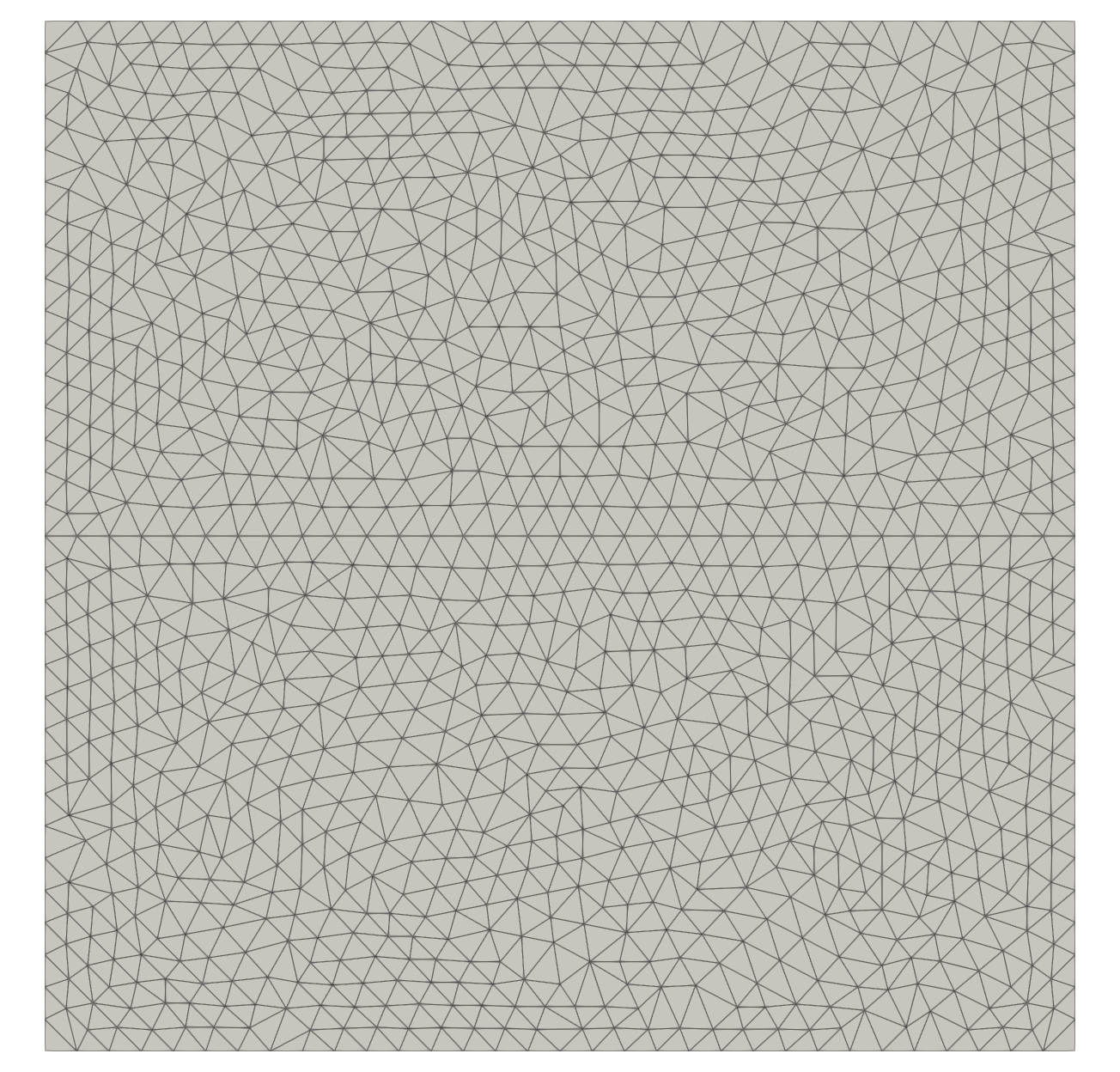
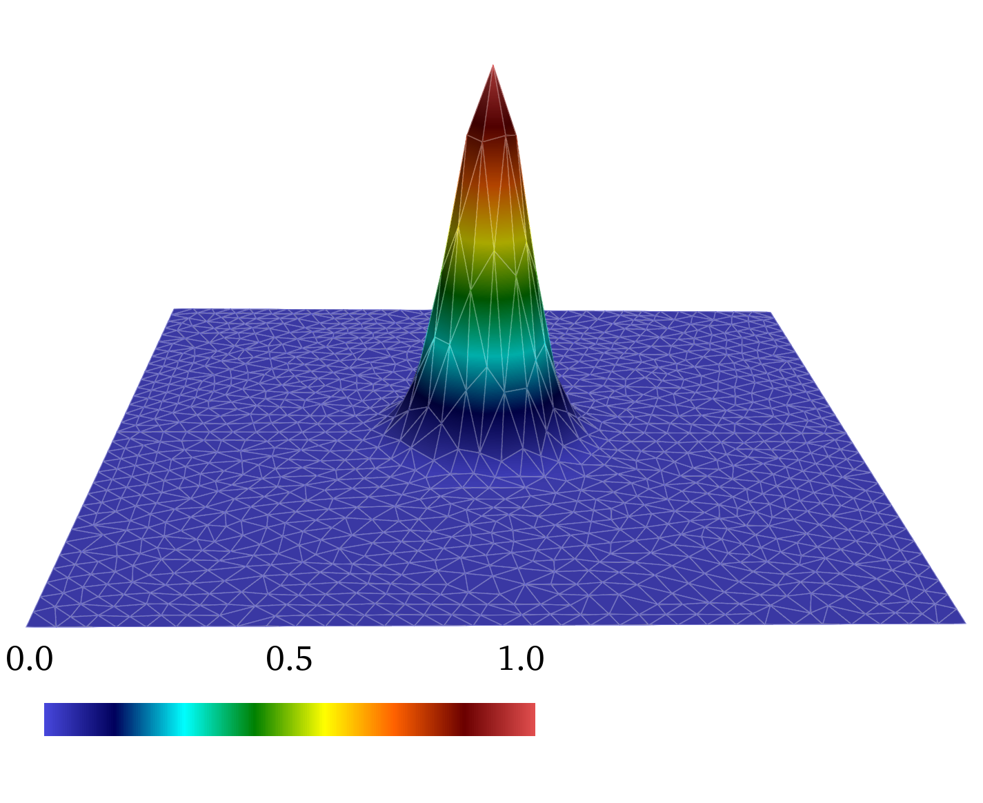
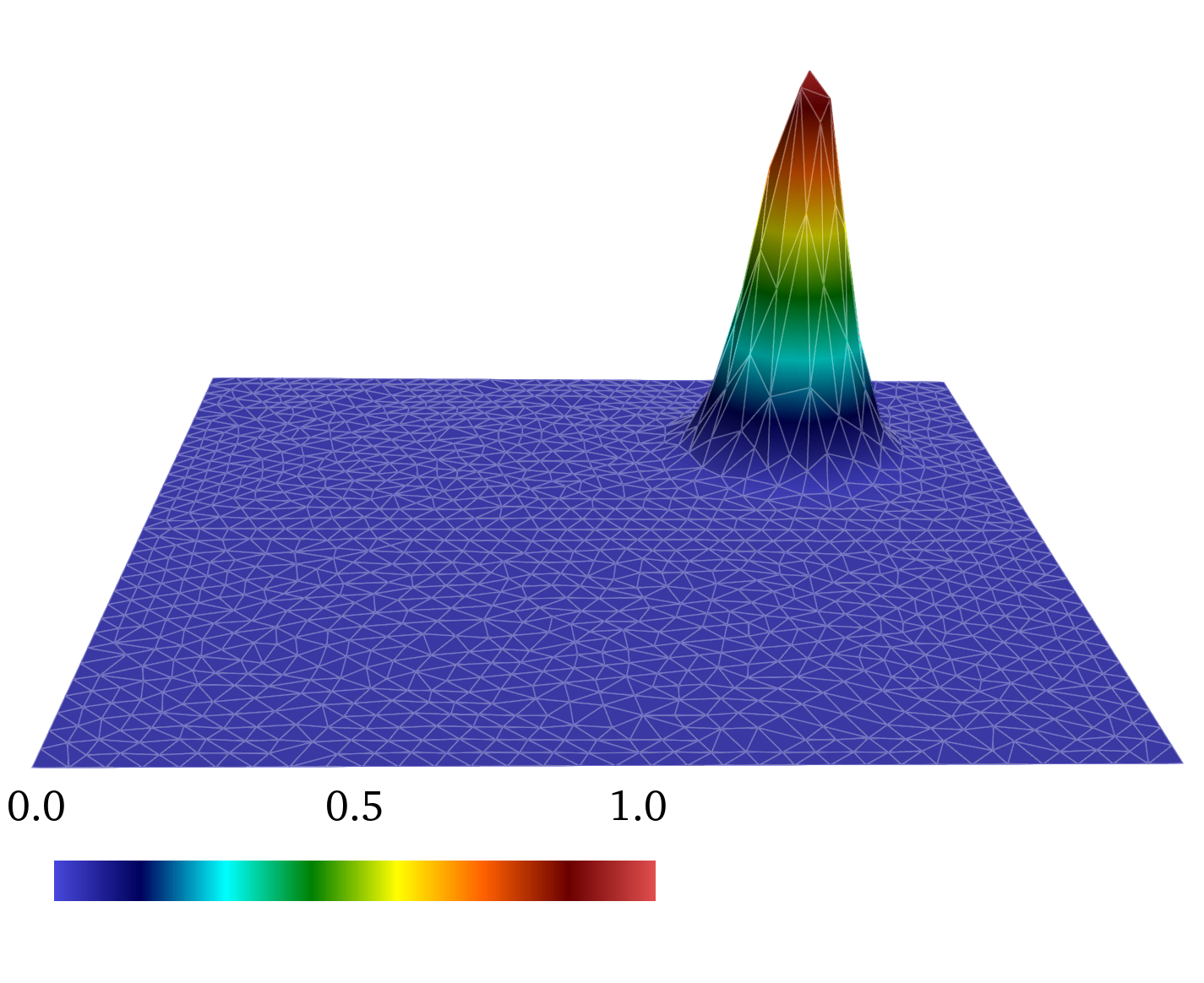
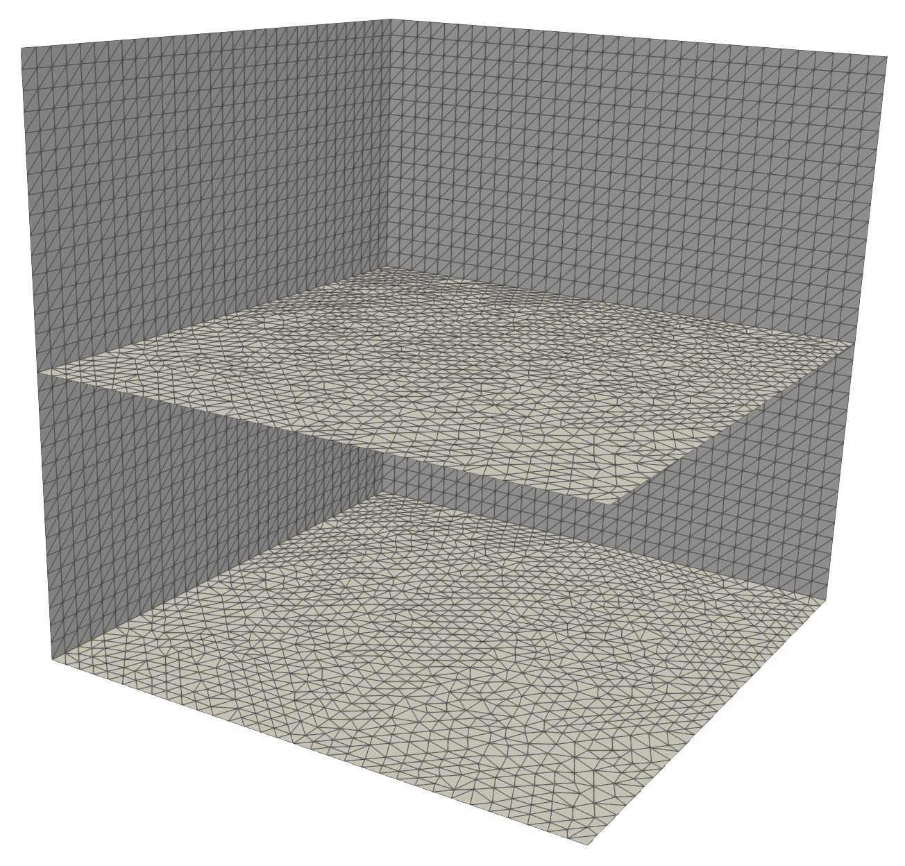
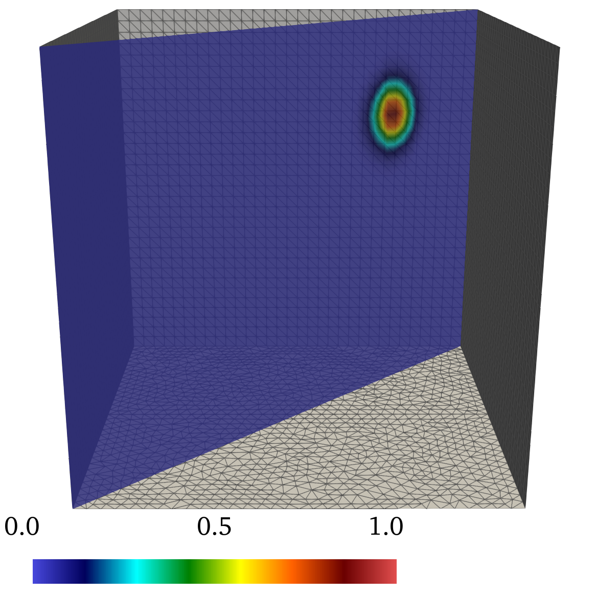
Figure 1: Employed meshes (left column) and numerical solutions of Example 1 for $d=2$ (top row) and $d=3$ (bottom row). Initial conditions (middle column) and numerical solutions at the final time $T=0.5$ (right column) computed by scheme (9) are shown.

Table 1: Relative errors and EOCs for $\Delta t=4h$ in 1D $(d=1)$.

$N$	$\Delta t$	$E_{\ell^{\infty}(L^{2})}$	EOC	$E_{\ell^{2}(H^{1}_{0})}$	EOC	$E_{\ell^{\infty}(H^{1}_{0})}$	EOC	$E_{\text{mass}}$
$32$	$2.50\times 10^{-1}$	$2.49\times 10^{-2}$	—	$4.05\times 10^{-2}$	—	$4.36\times 10^{-2}$	—	$1.39\times 10^{-3}$
$64$	$1.25\times 10^{-1}$	$9.02\times 10^{-3}$	$1.46$	$1.51\times 10^{-2}$	$1.43$	$1.60\times 10^{-2}$	$1.45$	$5.06\times 10^{-5}$
$128$	$6.25\times 10^{-2}$	$2.80\times 10^{-3}$	$1.69$	$4.65\times 10^{-3}$	$1.69$	$5.68\times 10^{-3}$	$1.49$	$1.93\times 10^{-5}$
$256$	$3.12\times 10^{-2}$	$8.09\times 10^{-4}$	$1.79$	$1.31\times 10^{-3}$	$1.83$	$1.80\times 10^{-3}$	$1.65$	$1.39\times 10^{-6}$
$512$	$1.56\times 10^{-2}$	$2.22\times 10^{-4}$	$1.86$	$3.47\times 10^{-4}$	$1.91$	$5.29\times 10^{-4}$	$1.76$	$1.53\times 10^{-6}$
$1{,}024$	$7.81\times 10^{-3}$	$5.93\times 10^{-5}$	$1.91$	$9.16\times 10^{-5}$	$1.92$	$1.47\times 10^{-4}$	$1.85$	$8.20\times 10^{-8}$
$2{,}048$	$3.91\times 10^{-3}$	$1.54\times 10^{-5}$	$1.95$	$2.52\times 10^{-5}$	$1.86$	$3.96\times 10^{-5}$	$1.90$	$7.99\times 10^{-8}$
$4{,}096$	$1.95\times 10^{-3}$	$3.95\times 10^{-6}$	$1.96$	$8.04\times 10^{-6}$	$1.64$	$1.05\times 10^{-5}$	$1.90$	$8.89\times 10^{-8}$
$8{,}192$	$9.77\times 10^{-4}$	$1.00\times 10^{-6}$	$1.98$	$3.25\times 10^{-6}$	$1.31$	$6.32\times 10^{-6}$	$0.74$	$9.19\times 10^{-8}$

Table 2: Relative errors and EOCs for $\Delta t=0.4\sqrt{h}$ in 1D $(d=1)$.

$N$	$\Delta t$	$E_{\ell^{\infty}(L^{2})}$	EOC	$E_{\ell^{2}(H^{1}_{0})}$	EOC	$E_{\ell^{\infty}(H^{1}_{0})}$	EOC	$E_{\text{mass}}$
$32$	$1.00\times 10^{-1}$	$9.51\times 10^{-3}$	—	$2.51\times 10^{-2}$	—	$3.36\times 10^{-2}$	—	$2.72\times 10^{-4}$
$64$	$7.07\times 10^{-2}$	$3.00\times 10^{-3}$	$3.33$	$5.71\times 10^{-3}$	$4.27$	$6.25\times 10^{-3}$	$4.85$	$4.87\times 10^{-5}$
$128$	$5.00\times 10^{-2}$	$1.82\times 10^{-3}$	$1.43$	$2.96\times 10^{-3}$	$1.89$	$3.79\times 10^{-3}$	$1.45$	$9.76\times 10^{-7}$
$256$	$3.54\times 10^{-2}$	$1.02\times 10^{-3}$	$1.67$	$1.69\times 10^{-3}$	$1.63$	$2.26\times 10^{-3}$	$1.50$	$5.33\times 10^{-8}$
$512$	$2.50\times 10^{-2}$	$5.49\times 10^{-4}$	$1.79$	$9.11\times 10^{-4}$	$1.77$	$1.25\times 10^{-3}$	$1.70$	$3.95\times 10^{-8}$
$1{,}024$	$1.77\times 10^{-2}$	$2.87\times 10^{-4}$	$1.88$	$4.78\times 10^{-4}$	$1.87$	$6.81\times 10^{-4}$	$1.76$	$6.71\times 10^{-8}$
$2{,}048$	$1.25\times 10^{-2}$	$1.49\times 10^{-4}$	$1.89$	$2.45\times 10^{-4}$	$1.92$	$3.61\times 10^{-4}$	$1.82$	$9.11\times 10^{-8}$
$4{,}096$	$8.84\times 10^{-3}$	$7.64\times 10^{-5}$	$1.92$	$1.25\times 10^{-4}$	$1.95$	$1.88\times 10^{-4}$	$1.88$	$7.40\times 10^{-8}$
$8{,}192$	$6.25\times 10^{-3}$	$3.90\times 10^{-5}$	$1.94$	$6.29\times 10^{-5}$	$1.97$	$9.72\times 10^{-5}$	$1.91$	$9.49\times 10^{-8}$

Table 3: Relative errors and EOCs for $\Delta t=h^{2/3}$ in 1D $(d=1)$.

$N$	$\Delta t$	$E_{\ell^{\infty}(L^{2})}$	EOC	$E_{\ell^{2}(H^{1}_{0})}$	EOC	$E_{\ell^{\infty}(H^{1}_{0})}$	EOC	$E_{\text{mass}}$
$32$	$1.57\times 10^{-1}$	$1.16\times 10^{-2}$	—	$2.19\times 10^{-2}$	—	$2.61\times 10^{-2}$	—	$5.43\times 10^{-5}$
$64$	$9.92\times 10^{-2}$	$5.89\times 10^{-3}$	$1.47$	$9.83\times 10^{-3}$	$1.74$	$1.06\times 10^{-2}$	$1.96$	$1.22\times 10^{-5}$
$128$	$6.25\times 10^{-2}$	$2.80\times 10^{-3}$	$1.61$	$4.65\times 10^{-3}$	$1.62$	$5.68\times 10^{-3}$	$1.36$	$1.93\times 10^{-5}$
$256$	$3.94\times 10^{-2}$	$1.26\times 10^{-3}$	$1.73$	$2.12\times 10^{-3}$	$1.71$	$2.74\times 10^{-3}$	$1.58$	$6.67\times 10^{-7}$
$512$	$2.48\times 10^{-2}$	$5.41\times 10^{-4}$	$1.82$	$8.98\times 10^{-4}$	$1.85$	$1.23\times 10^{-3}$	$1.73$	$5.75\times 10^{-8}$
$1{,}024$	$1.56\times 10^{-2}$	$2.27\times 10^{-4}$	$1.87$	$3.73\times 10^{-4}$	$1.90$	$5.43\times 10^{-4}$	$1.77$	$2.47\times 10^{-7}$
$2{,}048$	$9.84\times 10^{-3}$	$9.39\times 10^{-5}$	$1.91$	$1.53\times 10^{-4}$	$1.94$	$2.30\times 10^{-4}$	$1.86$	$6.44\times 10^{-8}$
$4{,}096$	$6.20\times 10^{-3}$	$3.83\times 10^{-5}$	$1.94$	$6.16\times 10^{-5}$	$1.97$	$9.57\times 10^{-5}$	$1.90$	$7.90\times 10^{-8}$
$8{,}192$	$3.91\times 10^{-3}$	$1.55\times 10^{-5}$	$1.96$	$2.47\times 10^{-5}$	$1.98$	$3.94\times 10^{-5}$	$1.92$	$9.47\times 10^{-8}$

Table 4: Relative errors and EOCs for $\Delta t=4h$ in 2D $(d=2)$.

$N$	$\Delta t$	$E_{\ell^{\infty}(L^{2})}$	EOC	$E_{\ell^{2}(H^{1}_{0})}$	EOC	$E_{\ell^{\infty}(H^{1}_{0})}$	EOC	$E_{\text{mass}}$
$32$	$2.50\times 10^{-1}$	$4.27\times 10^{-2}$	—	$7.29\times 10^{-2}$	—	$7.62\times 10^{-2}$	—	$3.66\times 10^{-3}$
$64$	$1.25\times 10^{-1}$	$1.42\times 10^{-2}$	$1.59$	$2.90\times 10^{-2}$	$1.33$	$3.10\times 10^{-2}$	$1.30$	$1.37\times 10^{-3}$
$128$	$6.25\times 10^{-2}$	$4.42\times 10^{-3}$	$1.69$	$1.20\times 10^{-2}$	$1.28$	$1.36\times 10^{-2}$	$1.19$	$9.18\times 10^{-5}$
$256$	$3.12\times 10^{-2}$	$1.28\times 10^{-3}$	$1.78$	$4.54\times 10^{-3}$	$1.40$	$5.31\times 10^{-3}$	$1.36$	$2.26\times 10^{-5}$
$512$	$1.56\times 10^{-2}$	$3.63\times 10^{-4}$	$1.82$	$2.45\times 10^{-3}$	$0.89$	$2.92\times 10^{-3}$	$0.86$	$5.31\times 10^{-6}$
$1{,}024$	$7.81\times 10^{-3}$	$9.78\times 10^{-5}$	$1.89$	$1.11\times 10^{-3}$	$1.14$	$1.41\times 10^{-3}$	$1.05$	$1.36\times 10^{-6}$
$2{,}048$	$3.91\times 10^{-3}$	$2.57\times 10^{-5}$	$1.93$	$5.62\times 10^{-4}$	$0.98$	$7.04\times 10^{-4}$	$1.01$	$6.97\times 10^{-7}$

Table 5: Relative errors and EOCs for $\Delta t=0.4\sqrt{h}$ in 2D $(d=2)$.

$N$	$\Delta t$	$E_{\ell^{\infty}(L^{2})}$	EOC	$E_{\ell^{2}(H^{1}_{0})}$	EOC	$E_{\ell^{\infty}(H^{1}_{0})}$	EOC	$E_{\text{mass}}$
$32$	$1.00\times 10^{-1}$	$2.06\times 10^{-2}$	—	$5.52\times 10^{-2}$	—	$7.34\times 10^{-2}$	—	$2.41\times 10^{-3}$
$64$	$7.07\times 10^{-2}$	$5.57\times 10^{-3}$	$3.77$	$2.25\times 10^{-2}$	$2.58$	$2.61\times 10^{-2}$	$2.99$	$8.04\times 10^{-4}$
$128$	$5.00\times 10^{-2}$	$3.00\times 10^{-3}$	$1.79$	$1.10\times 10^{-2}$	$2.07$	$1.32\times 10^{-2}$	$1.96$	$1.25\times 10^{-4}$
$256$	$3.54\times 10^{-2}$	$1.62\times 10^{-3}$	$1.78$	$4.75\times 10^{-3}$	$2.42$	$5.43\times 10^{-3}$	$2.57$	$2.47\times 10^{-5}$
$512$	$2.50\times 10^{-2}$	$8.80\times 10^{-4}$	$1.76$	$2.69\times 10^{-3}$	$1.64$	$3.05\times 10^{-3}$	$1.67$	$9.88\times 10^{-6}$
$1{,}024$	$1.77\times 10^{-2}$	$4.66\times 10^{-4}$	$1.84$	$1.26\times 10^{-3}$	$2.18$	$1.49\times 10^{-3}$	$2.07$	$2.67\times 10^{-6}$
$2{,}048$	$1.25\times 10^{-2}$	$2.43\times 10^{-4}$	$1.87$	$6.45\times 10^{-4}$	$1.94$	$7.43\times 10^{-4}$	$2.00$	$8.11\times 10^{-7}$

Table 6: Relative errors and EOCs for $\Delta t=h^{2/3}$ in 2D $(d=2)$.

$N$	$\Delta t$	$E_{\ell^{\infty}(L^{2})}$	EOC	$E_{\ell^{2}(H^{1}_{0})}$	EOC	$E_{\ell^{\infty}(H^{1}_{0})}$	EOC	$E_{\text{mass}}$
$32$	$1.57\times 10^{-1}$	$2.24\times 10^{-2}$	—	$5.09\times 10^{-2}$	—	$5.80\times 10^{-2}$	—	$1.34\times 10^{-3}$
$64$	$9.92\times 10^{-2}$	$9.76\times 10^{-3}$	$1.80$	$2.46\times 10^{-2}$	$1.58$	$2.63\times 10^{-2}$	$1.71$	$1.23\times 10^{-3}$
$128$	$6.25\times 10^{-2}$	$4.42\times 10^{-3}$	$1.72$	$1.19\times 10^{-2}$	$1.57$	$1.36\times 10^{-2}$	$1.43$	$3.62\times 10^{-5}$
$256$	$3.94\times 10^{-2}$	$1.97\times 10^{-3}$	$1.75$	$5.04\times 10^{-3}$	$1.86$	$5.59\times 10^{-3}$	$1.93$	$1.91\times 10^{-5}$
$512$	$2.48\times 10^{-2}$	$8.67\times 10^{-4}$	$1.77$	$2.68\times 10^{-3}$	$1.37$	$3.04\times 10^{-3}$	$1.32$	$9.60\times 10^{-6}$
$1{,}024$	$1.56\times 10^{-2}$	$3.70\times 10^{-4}$	$1.85$	$1.21\times 10^{-3}$	$1.73$	$1.46\times 10^{-3}$	$1.59$	$2.91\times 10^{-6}$
$2{,}048$	$9.84\times 10^{-3}$	$1.54\times 10^{-4}$	$1.89$	$5.95\times 10^{-4}$	$1.53$	$7.19\times 10^{-4}$	$1.53$	$7.92\times 10^{-7}$

Table 7: Relative errors and EOCs for $\Delta t=2h$ in 3D $(d=3)$.

$N$	$\Delta t$	$E_{\ell^{\infty}(L^{2})}$	EOC	$E_{\ell^{2}(H^{1}_{0})}$	EOC	$E_{\ell^{\infty}(H^{1}_{0})}$	EOC	$E_{\text{mass}}$
32	$1.25\times 10^{-1}$	$4.41\times 10^{-2}$	—	$8.15\times 10^{-2}$	—	$1.01\times 10^{-1}$	—	$2.70\times 10^{-3}$
64	$6.25\times 10^{-2}$	$1.19\times 10^{-2}$	1.89	$2.72\times 10^{-2}$	1.58	$3.26\times 10^{-2}$	1.64	$1.28\times 10^{-3}$
128	$3.13\times 10^{-2}$	$3.04\times 10^{-3}$	1.97	$1.07\times 10^{-2}$	1.34	$1.29\times 10^{-2}$	1.33	$1.05\times 10^{-4}$
256	$1.56\times 10^{-2}$	$7.51\times 10^{-4}$	2.02	$4.05\times 10^{-3}$	1.41	$4.89\times 10^{-3}$	1.40	$3.48\times 10^{-5}$

Table 8: Relative errors and EOCs for $\Delta t=4h$ in 3D $(d=3)$.

$N$	$\Delta t$	$E_{\ell^{\infty}(L^{2})}$	EOC	$E_{\ell^{2}(H^{1}_{0})}$	EOC	$E_{\ell^{\infty}(H^{1}_{0})}$	EOC	$E_{\text{mass}}$
$32$	$2.50\times 10^{-1}$	$6.28\times 10^{-2}$	—	$9.12\times 10^{-2}$	—	$9.79\times 10^{-2}$	—	$3.08\times 10^{-3}$
$64$	$1.25\times 10^{-1}$	$1.92\times 10^{-2}$	$1.71$	$3.30\times 10^{-2}$	$1.47$	$3.40\times 10^{-2}$	$1.53$	$1.46\times 10^{-3}$
$128$	$6.25\times 10^{-2}$	$5.81\times 10^{-3}$	$1.73$	$1.26\times 10^{-2}$	$1.39$	$1.35\times 10^{-2}$	$1.33$	$1.38\times 10^{-4}$
$256$	$3.12\times 10^{-2}$	$1.78\times 10^{-3}$	$1.70$	$4.48\times 10^{-3}$	$1.49$	$5.01\times 10^{-3}$	$1.43$	$3.53\times 10^{-5}$

Table 9: Relative errors and EOCs for $\Delta t=0.2\sqrt{h}$ in 3D $(d=3)$.

$N$	$\Delta t$	$E_{\ell^{\infty}(L^{2})}$	EOC	$E_{\ell^{2}(H^{1}_{0})}$	EOC	$E_{\ell^{\infty}(H^{1}_{0})}$	EOC	$E_{\text{mass}}$
32	$5.00\times 10^{-2}$	$5.33\times 10^{-2}$	—	$1.00\times 10^{-1}$	—	$1.24\times 10^{-1}$	—	$8.03\times 10^{-3}$
64	$3.54\times 10^{-2}$	$1.25\times 10^{-2}$	4.19	$2.86\times 10^{-2}$	3.61	$3.46\times 10^{-2}$	3.69	$1.99\times 10^{-3}$
128	$2.50\times 10^{-2}$	$3.08\times 10^{-3}$	4.03	$1.07\times 10^{-2}$	2.83	$1.30\times 10^{-2}$	2.83	$1.13\times 10^{-4}$
256	$1.77\times 10^{-2}$	$8.44\times 10^{-4}$	3.74	$4.08\times 10^{-3}$	2.79	$4.90\times 10^{-3}$	2.81	$3.15\times 10^{-5}$

Table 10: Relative errors and EOCs for $\Delta t=0.4\sqrt{h}$ in 3D $(d=3)$.

$N$	$\Delta t$	$E_{\ell^{\infty}(L^{2})}$	EOC	$E_{\ell^{2}(H^{1}_{0})}$	EOC	$E_{\ell^{\infty}(H^{1}_{0})}$	EOC	$E_{\text{mass}}$
$32$	$1.00\times 10^{-1}$	$4.60\times 10^{-2}$	—	$8.66\times 10^{-2}$	—	$1.10\times 10^{-1}$	—	$1.03\times 10^{-3}$
$64$	$7.07\times 10^{-2}$	$1.25\times 10^{-2}$	$3.75$	$2.74\times 10^{-2}$	$3.32$	$3.30\times 10^{-2}$	$3.46$	$1.29\times 10^{-3}$
$128$	$5.00\times 10^{-2}$	$3.91\times 10^{-3}$	$3.36$	$1.14\times 10^{-2}$	$2.54$	$1.32\times 10^{-2}$	$2.64$	$1.59\times 10^{-4}$
$256$	$3.54\times 10^{-2}$	$2.24\times 10^{-3}$	$1.61$	$4.77\times 10^{-3}$	$2.51$	$5.13\times 10^{-3}$	$2.73$	$1.76\times 10^{-5}$

Table 11: Relative errors and EOCs for $\Delta t=h^{2/3}$ in 3D $(d=3)$.

$N$	$\Delta t$	$E_{\ell^{\infty}(L^{2})}$	EOC	$E_{\ell^{2}(H^{1}_{0})}$	EOC	$E_{\ell^{\infty}(H^{1}_{0})}$	EOC	$E_{\text{mass}}$
32	$1.57\times 10^{-1}$	$4.61\times 10^{-2}$	—	$7.82\times 10^{-2}$	—	$9.86\times 10^{-2}$	—	$2.02\times 10^{-4}$
64	$9.92\times 10^{-2}$	$1.48\times 10^{-2}$	$2.46$	$2.87\times 10^{-2}$	$2.17$	$3.19\times 10^{-2}$	$2.44$	$1.30\times 10^{-3}$
128	$6.25\times 10^{-2}$	$5.81\times 10^{-3}$	$2.02$	$1.26\times 10^{-2}$	$1.78$	$1.35\times 10^{-2}$	$1.86$	$1.38\times 10^{-4}$
256	$3.94\times 10^{-2}$	$2.72\times 10^{-3}$	$1.64$	$5.19\times 10^{-3}$	$1.92$	$5.81\times 10^{-3}$	$1.82$	$2.30\times 10^{-5}$

Table 12: Relative errors and EOCs for $N=256$ in 2D $(d=2)$ for $\nu=10^{-2}$.

$N$	$\Delta t$	$E_{\ell^{\infty}(L^{2})}$	EOC	$E_{\ell^{2}(H^{1}_{0})}$	EOC	$E_{\ell^{\infty}(H^{1}_{0})}$	EOC	$E_{\text{mass}}$
256	$2.50\times 10^{-1}$	$4.56\times 10^{-2}$	—	$6.45\times 10^{-2}$	—	$6.63\times 10^{-2}$	—	$4.79\times 10^{-5}$
256	$1.25\times 10^{-1}$	$1.49\times 10^{-2}$	1.62	$2.27\times 10^{-2}$	1.51	$2.53\times 10^{-2}$	1.39	$2.41\times 10^{-5}$
256	$6.25\times 10^{-2}$	$4.48\times 10^{-3}$	1.73	$7.80\times 10^{-3}$	1.54	$9.01\times 10^{-3}$	1.49	$2.79\times 10^{-5}$
256	$3.13\times 10^{-2}$	$1.28\times 10^{-3}$	1.80	$4.54\times 10^{-3}$	0.78	$5.31\times 10^{-3}$	0.76	$2.26\times 10^{-5}$
256	$1.56\times 10^{-2}$	$3.70\times 10^{-4}$	1.80	$4.23\times 10^{-3}$	0.10	$5.17\times 10^{-3}$	0.04	$1.41\times 10^{-4}$
256	$7.81\times 10^{-3}$	$6.88\times 10^{-4}$	-0.90	$4.23\times 10^{-3}$	0.00	$5.14\times 10^{-3}$	0.01	$6.38\times 10^{-4}$
256	$3.91\times 10^{-3}$	$8.81\times 10^{-4}$	-0.36	$4.53\times 10^{-3}$	-0.10	$5.41\times 10^{-3}$	-0.08	$8.33\times 10^{-5}$

Table 13: Relative errors and EOCs in $h$ (denoted by EOC_h in the table) for $\Delta t=0.01$ in 2D $(d=2)$ for $\nu=10^{-2}$.

$N$	$\Delta t$	$E_{\ell^{\infty}(L^{2})}$	EOCh	$E_{\ell^{2}(H^{1}_{0})}$	EOCh	$E_{\ell^{\infty}(H^{1}_{0})}$	EOCh	$E_{\text{mass}}$
32	$0.01$	$4.79\times 10^{-2}$	—	$1.07\times 10^{-1}$	—	$1.34\times 10^{-1}$	—	$5.25\times 10^{-4}$
64	$0.01$	$9.48\times 10^{-3}$	$2.34$	$2.98\times 10^{-2}$	$1.84$	$3.61\times 10^{-2}$		$1.04\times 10^{-3}$
128	$0.01$	$1.79\times 10^{-3}$	$2.40$	$1.08\times 10^{-2}$	$1.46$	$1.35\times 10^{-2}$	$1.42$	$1.99\times 10^{-5}$
256	$0.01$	$3.14\times 10^{-4}$	$2.51$	$4.21\times 10^{-3}$	$1.36$	$5.16\times 10^{-3}$	$1.39$	$1.86\times 10^{-4}$
512	$0.01$	$1.53\times 10^{-4}$	$1.04$	$2.41\times 10^{-3}$	$0.80$	$2.91\times 10^{-3}$	$0.83$	$9.85\times 10^{-6}$
1024	$0.01$	$1.58\times 10^{-4}$	$-0.05$	$1.12\times 10^{-3}$	$1.11$	$1.42\times 10^{-3}$	$1.04$	$3.04\times 10^{-6}$
2048	$0.01$	$1.59\times 10^{-4}$	$-0.01$	$5.98\times 10^{-4}$	$0.91$	$7.20\times 10^{-4}$	$0.98$	$7.99\times 10^{-7}$

Table 14: Relative errors of mass for $\Delta t=4h$ in 2D $(d=2)$.

$N$	$\Delta t$	$E_{\text{mass}}$	$E_{\text{mass}}^{\prime}$	$E_{\text{mass}}^{\prime\prime}$
32	$2.50\times 10^{-1}$	$3.66\times 10^{-3}$	$1.36\times 10^{-3}$	$3.83\times 10^{-3}$
64	$1.25\times 10^{-1}$	$1.37\times 10^{-3}$	$9.23\times 10^{-5}$	$1.08\times 10^{-3}$
128	$6.25\times 10^{-2}$	$9.18\times 10^{-5}$	$4.11\times 10^{-5}$	$1.50\times 10^{-4}$
256	$3.13\times 10^{-2}$	$2.26\times 10^{-5}$	$2.30\times 10^{-6}$	$2.56\times 10^{-5}$
512	$1.56\times 10^{-2}$	$5.31\times 10^{-6}$	$3.43\times 10^{-6}$	$6.29\times 10^{-6}$
1024	$7.81\times 10^{-3}$	$1.36\times 10^{-6}$	$6.49\times 10^{-7}$	$1.23\times 10^{-6}$
2048	$3.91\times 10^{-3}$	$6.97\times 10^{-7}$	$5.03\times 10^{-7}$	$3.45\times 10^{-7}$

Table 15: Relative errors and EOCs for $\Delta t=4h$ in 2D $(d=2)$ for $\nu=10^{-3}$.

$N$	$\Delta t$	$E_{\ell^{\infty}(L^{2})}$	EOC	$E_{\ell^{2}(H^{1}_{0})}$	EOC	$E_{\ell^{\infty}(H^{1}_{0})}$	EOC	$E_{\text{mass}}$
32	$2.50\times 10^{-1}$	$1.91\times 10^{-1}$	—	$2.46\times 10^{-1}$	—	$2.65\times 10^{-1}$	—	$4.59\times 10^{-2}$
64	$1.25\times 10^{-1}$	$4.50\times 10^{-2}$	2.09	$1.02\times 10^{-1}$	1.26	$1.33\times 10^{-1}$	0.99	$6.15\times 10^{-3}$
128	$6.25\times 10^{-2}$	$1.35\times 10^{-2}$	1.74	$3.71\times 10^{-2}$	1.47	$4.92\times 10^{-2}$	1.43	$3.72\times 10^{-3}$
256	$3.13\times 10^{-2}$	$3.25\times 10^{-3}$	2.05	$1.47\times 10^{-2}$	1.33	$1.98\times 10^{-2}$	1.31	$1.33\times 10^{-3}$
512	$1.56\times 10^{-2}$	$8.46\times 10^{-4}$	1.94	$7.66\times 10^{-3}$	0.94	$9.75\times 10^{-3}$	1.02	$5.51\times 10^{-4}$
1024	$7.81\times 10^{-3}$	$3.31\times 10^{-4}$	1.35	$3.40\times 10^{-3}$	1.17	$4.82\times 10^{-3}$	1.02	$3.03\times 10^{-4}$
2048	$3.91\times 10^{-3}$	$1.18\times 10^{-4}$	1.49	$1.74\times 10^{-3}$	0.97	$2.38\times 10^{-3}$	1.02	$1.13\times 10^{-4}$

Table 16: Relative errors and EOCs for $\Delta t=4h$ in 2D $(d=2)$ for $\nu=10^{-4}$.

$N$	$\Delta t$	$E_{\ell^{\infty}(L^{2})}$	EOC	$E_{\ell^{2}(H^{1}_{0})}$	EOC	$E_{\ell^{\infty}(H^{1}_{0})}$	EOC	$E_{\text{mass}}$
32	$2.50\times 10^{-1}$	$3.27\times 10^{+1}$	—	$4.63\times 10^{+1}$	—	$3.41\times 10^{+1}$	—	$1.08\times 10^{+2}$
64	$1.25\times 10^{-1}$	$9.51\times 10^{-1}$	5.11	$1.03\times 10^{-0}$	5.50	$1.06\times 10^{0}$	5.01	$5.70\times 10^{-1}$
128	$6.25\times 10^{-2}$	$1.84\times 10^{-1}$	2.37	$3.41\times 10^{-1}$	1.59	$4.11\times 10^{-1}$	1.37	$3.47\times 10^{-2}$
256	$3.13\times 10^{-2}$	$5.44\times 10^{-2}$	1.76	$1.07\times 10^{-1}$	1.67	$1.50\times 10^{-1}$	1.45	$5.82\times 10^{-3}$
512	$1.56\times 10^{-2}$	$1.04\times 10^{-2}$	2.38	$3.51\times 10^{-2}$	1.61	$4.48\times 10^{-2}$	1.75	$2.61\times 10^{-3}$
1024	$7.81\times 10^{-3}$	$2.69\times 10^{-3}$	1.95	$1.31\times 10^{-2}$	1.42	$1.88\times 10^{-2}$	1.25	$1.08\times 10^{-3}$
2048	$3.91\times 10^{-3}$	$9.54\times 10^{-4}$	1.50	$5.98\times 10^{-3}$	1.13	$8.24\times 10^{-3}$	1.19	$1.69\times 10^{-4}$

6 Conclusions

We have presented a mass-preserving two-step Lagrange–Galerkin scheme of second order in time for convection-diffusion problems. Its mass-preserving property is achieved by the Jacobian multiplication technique, and its accuracy of second order in time is obtained based on the idea of the multistep Galerkin method along characteristics. For the first time step, we have proposed to employ a mass-preserving scheme of first order in time. This construction is efficient and does not decrease the convergence orders in the $\ell^{\infty}(L^{2})$- and $\ell^{2}(H^{1}_{0})$-norms.

Both main advantages of Lagrange–Galerkin methods, the CFL-free robustness for convection-dominated problems and the symmetric and positive coefficient matrix of the resulting system of linear equations, are kept in our scheme. Additionally, our scheme has a mass-preserving property as proved in Theorem 1. We have proved unconditional stability without any stabilization parameter in Theorem 2, and error estimates of second order in time in Theorem 3. For the error estimates two key lemmas on the truncation error analysis of the material derivative in conservative form, cf. Lemma 4, and a discrete Gronwall inequality for multistep methods, cf. Lemma 1, have been prepared.

We summarize the shown convergence orders as follows. The order in the $\ell^{\infty}(L^{2})\cap\ell^{2}(H^{1}_{0})$-norm is $O(\Delta t^{2}+h^{k})$, and the order in the $\ell^{\infty}(L^{2})$-norm is $O(\Delta t^{2}+h^{k+1})$ if the duality argument can be employed. We have also proved the convergence order $O(\Delta t^{3/2}+h^{k})$ in the discrete $\ell^{\infty}(H^{1}_{0})$- and $H^{1}(L^{2})$-norm, which will be useful when we apply the scheme to, e.g., the Navier–Stokes equations. We have presented numerical results in one-, two- and three-dimensions, which have supported the theoretical convergence orders.

Appendix

A.1 Proof of Lemma 1

From the assumption (20), there exists a non-negative sequence $\{\tilde{z}_{n}\}_{n\geq 2}$ such that

$$\frac{1}{\Delta t}\Bigl{(}\frac{3}{2}x_{n}-2x_{n-1}+\frac{1}{2}x_{n-2}+y_{n}-y_{n-1}\Bigr{)}+\tilde{z}_{n}=a_{0}x_{n}+a_{1}x_{n-1}+a_{2}x_{n-2}+b_{n},\quad\forall n\geq 2,$$

where $\tilde{z}_{n}$ satisfies

$$z_{n}\leq\tilde{z}_{n},\quad\forall n\geq 2.$$

Let $p$ and $q$, $p<q$, be the roots of quadratic equation $f(x)\coloneqq(3/2-a_{0}\Delta t)x^{2}-(2+a_{1}\Delta t)x+(1/2-a_{2}\Delta t)=0$, and let $\lambda\coloneqq 2/3$ and $D\coloneqq(2+a_{1}\Delta t)^{2}-(3-2a_{0}\Delta t)(1-2a_{2}\Delta t)$ $(=1+2(a_{0}+2a_{1}+3a_{2})\Delta t+(a_{1}^{2}-4a_{0}a_{2})\Delta t^{2})$. The numbers $p$ and $q$ have the properties

$$|p| <1\leq q, 2\lambda \leq p+q, pq \leq\lambda, q-p \geq\lambda, q^{n}-p^{n} \leq\exp(2a_{\ast}n\Delta t)+1,$$ (A.1)

which are obtained from $f(1)=-(a_{0}+a_{1}+a_{2})\Delta t\leq 0$, $f(-1)=4+(-a_{0}+a_{1}-a_{2})\Delta t\geq{{}13/4}>0$, $a_{0}\Delta t\leq 3/4$, $1\leq D\leq[1+(a_{0}+2a_{1}+3a_{2})\Delta t]^{2}$, and

$$q^{n}-p^{n} \leq q^{n}+|p|^{n}\leq q^{n}+1=\left(\frac{2+a_{1}\Delta t+\sqrt{D}}{3-2a_{0}\Delta t}\right)^{n}+1\leq\left(1+\frac{3a_{\ast}\Delta t}{3-2a_{0}\Delta t}\right)^{n}+1$$

$$\leq(1+2a_{\ast}\Delta t)^{n}{{}+1}\leq\exp(2a_{\ast}n\Delta t){{}+1.}$$

Let $n\geq 2$ be fixed arbitrarily. Then, we have

$$x_{n}-px_{n-1}+\lambda(y_{n}-y_{n-1})+\lambda\Delta t\tilde{z}_{n} =q(x_{n-1}-px_{n-2})+\lambda\Delta tb_{n},$$

$$x_{n}-qx_{n-1}+\lambda(y_{n}-y_{n-1})+\lambda\Delta t\tilde{z}_{n} =p(x_{n-1}-qx_{n-2})+\lambda\Delta tb_{n},$$

which imply

$$x_{n}-px_{n-1}+\lambda\Biggl{[}\sum_{i=2}^{n}q^{n-i}y_{i}-\sum_{i=1}^{n-1}q^{n-1-i}y_{i}\Biggr{]}+\lambda\Delta t\sum_{i=2}^{n}q^{n-i}\tilde{z}_{i} =q^{n-1}(x_{1}-px_{0})+\lambda\Delta t\sum_{i=2}^{n}q^{n-i}b_{i},$$ (A.2a)

$$x_{n}-qx_{n-1}+\lambda\Biggl{[}\sum_{i=2}^{n}p^{n-i}y_{i}-\sum_{i=1}^{n-1}p^{n-1-i}y_{i}\Biggr{]}+\lambda\Delta t\sum_{i=2}^{n}p^{n-i}\tilde{z}_{i} =p^{n-1}(x_{1}-qx_{0})+\lambda\Delta t\sum_{i=2}^{n}p^{n-i}b_{i}.$$ (A.2b)

Multiplying (A.2a) by $q$ and (A.2b) by $p$ and subtracting the second equation from the first, we get

$$(q-p)x_{n} +\lambda\Biggl{[}\sum_{i=2}^{n}(q^{n+1-i}-p^{n+1-i})y_{i}-\sum_{i=1}^{n-1}(q^{n-i}-p^{n-i})y_{i}\Biggr{]}+\lambda\Delta t\sum_{i=2}^{n}(q^{n+1-i}-p^{n+1-i})\tilde{z}_{i}$$

$$=(q^{n}-p^{n})x_{1}-pq(q^{n-1}-p^{n-1})x_{0}+\lambda\Delta t\sum_{i=2}^{n}(q^{n+1-i}-p^{n+1-i})b_{i}.$$ (A.3)

It is noted here that

$$\sum_{i=2}^{n}(q^{n+1-i} -p^{n+1-i})y_{i}-\sum_{i=1}^{n-1}(q^{n-i}-p^{n-i})y_{i}$$

$$=(q-p)y_{n}+\sum_{i=2}^{n-1}\Bigl{[}(q^{n+1-i}-p^{n+1-i})-(q^{n-i}-p^{n-i})\Bigr{]}y_{i}-(q^{n-1}-p^{n-1})y_{1}$$

$$\geq(q-p)y_{n}-(q^{n-1}-p^{n-1})y_{1},$$ (A.4)

where the following inequality has been employed:

$$q^{k+1}-p^{k+1}\geq q^{k}-p^{k},\qquad\forall k\in\mathbb{N}\cup\{0\}.$$

This inequality holds obviously from the first property in (A.1) for $p\geq 0$ or for $p<0$ and an even number $k$. For $p<0$ and an odd number $k$, it is proved by induction, and the key inequality in the induction is

$$q^{k+2}-p^{k+2}=(q^{k+1}-p^{k+1})(p+q)-pq(q^{k}-p^{k})\geq(q^{k+1}-p^{k+1})(p+q)\geq q^{k+1}-p^{k+1}.$$

Combining (A.1) and (A.4) with (A.3) and noting that $0\leq-pq/(q-p)\leq q/(q-p)\leq 1$ for $p\in(-1,0)$ and $-pq/(q-p)\leq 0<1$ for $p\in[0,1)$, we obtain

$$x_{n}+\lambda y_{n}+\lambda\Delta t\sum_{i=2}^{n}\tilde{z}_{i} \leq\frac{q^{n}-p^{n}}{q-p}\Biggl{[}x_{1}-pqx_{0}+\lambda y_{1}+\lambda\Delta t\sum_{i=2}^{n}b_{i}\Biggr{]}$$

$$\leq\Bigl{(}\exp(2a_{\ast}n\Delta t)+1\Bigr{)}\Biggl{(}x_{0}+\frac{3}{2}x_{1}+y_{1}+\Delta t\sum_{i=2}^{n}b_{i}\Biggr{)},$$

which completes the proof.

A.2 Proof of Lemma 5

We prove (i). For the estimate (39a), from the next calculations,

$$\eta(\cdot,t) =\frac{1}{\Delta t}\int_{t^{n-1}}^{t^{n}}\eta(\cdot,t)\,ds=\frac{1}{\Delta t}\int_{t^{n-1}}^{t^{n}}\Bigl{(}\bigl{[}\eta(\cdot,s_{1})\bigr{]}_{s_{1}=s}^{t}\Bigr{)}ds+\frac{1}{\Delta t}\int_{t^{n-1}}^{t^{n}}\eta(\cdot,s)\,ds$$

$$=\frac{1}{\Delta t}\int_{t^{n-1}}^{t^{n}}ds\int_{s}^{t}\frac{\partial{\eta}}{\partial{t}}(\cdot,s_{1})\,ds_{1}+\frac{1}{\Delta t}\Bigl{[}\int_{t^{n-1}}^{t^{n}}\eta(\cdot,s)^{2}ds\Bigr{]}^{1/2}\Bigl{[}\int_{t^{n-1}}^{t^{n}}1^{2}ds\Bigr{]}^{1/2}$$

$$\leq\frac{1}{\Delta t}\int_{t^{n-1}}^{t^{n}}ds\Bigl{[}\int_{s}^{t}\frac{\partial{\eta}}{\partial{t}}(\cdot,s_{1})^{2}ds_{1}\Bigr{]}^{1/2}\Bigl{[}\int_{s}^{t}1^{2}ds_{1}\Bigr{]}^{1/2}+\frac{1}{\sqrt{\Delta t}}\Bigl{[}\int_{t^{n-1}}^{t^{n}}\eta(\cdot,s)^{2}ds\Bigr{]}^{1/2}$$

$$\leq\frac{1}{\Delta t}\int_{t^{n-1}}^{t^{n}}ds\Bigl{[}\int_{t^{n-1}}^{t^{n}}\frac{\partial{\eta}}{\partial{t}}(\cdot,s_{1})^{2}ds_{1}\Bigr{]}^{1/2}\Bigl{[}\int_{t^{n-1}}^{t^{n}}1^{2}ds_{1}\Bigr{]}^{1/2}+\frac{1}{\sqrt{\Delta t}}\Bigl{[}\int_{t^{n-1}}^{t^{n}}\eta(\cdot,s)^{2}ds\Bigr{]}^{1/2}$$

$$=\sqrt{\Delta t}\Bigl{[}\int_{t^{n-1}}^{t^{n}}\frac{\partial{\eta}}{\partial{t}}(\cdot,s)^{2}ds\Bigr{]}^{1/2}+\frac{1}{\sqrt{\Delta t}}\Bigl{[}\int_{t^{n-1}}^{t^{n}}\eta(\cdot,s)^{2}ds\Bigr{]}^{1/2}$$

$$\leq\sqrt{\frac{2}{\Delta t}}\,\Bigl{[}\int_{t^{n-1}}^{t^{n}}\Bigl{(}\eta(\cdot,s)^{2}+\frac{\partial{\eta}}{\partial{t}}(\cdot,s)^{2}\Bigr{)}ds\Bigr{]}^{1/2},$$

and Lemma 3-(i), we obtain the inequalities as

$$\|\eta(\cdot,t)\| \leq\|\eta(\cdot,t)\|_{H^{1}(\Omega)}\leq\sqrt{2}\,\Delta t^{-1/2}\|\eta\|_{H^{1}(t^{n-1},t^{n};H^{1})}\leq ch^{k}\Delta t^{-1/2}\|\phi\|_{H^{1}(t^{n-1},t^{n};H^{k+1})}$$

$$\leq c^{\prime}h^{k}\|\phi\|_{H^{2}(0,T;H^{k+1})}\quad\mbox{(by the Sobolev embedding theorem with respect to time).}$$

For the estimate (39b), noting that

$$\bigl{\|}\bar{D}_{\Delta t}^{(1)}\eta^{n}\bigr{\|} =\frac{1}{\Delta t}\|\eta^{n}-\eta^{n-1}\|\leq\frac{1}{\Delta t}\,\Bigl{\|}\bigl{[}\eta(\cdot,s)\bigr{]}_{s=t^{n-1}}^{t^{n}}\Bigr{\|}=\frac{1}{\Delta t}\Bigl{\|}\int_{t^{n-1}}^{t^{n}}\frac{\partial{\eta}}{\partial{t}}(\cdot,s)\,ds\Bigr{\|}$$

$$\leq\frac{1}{\Delta t}\int_{t^{n-1}}^{t^{n}}\Bigl{\|}\frac{\partial{\eta}}{\partial{t}}(\cdot,s)\Bigr{\|}\,ds\leq\frac{1}{\sqrt{\Delta t}}\,\Bigl{\|}\frac{\partial{\eta}}{\partial{t}}\Bigr{\|}_{L^{2}(t^{n-1},t^{n};L^{2}(\Omega))}$$

$$\leq\Delta t^{-1/2}\|\eta\|_{H^{1}(t^{n-1},t^{n};L^{2}(\Omega))}\leq ch^{k}\Delta t^{-1/2}\|\phi\|_{H^{1}(t^{n-1},t^{n};H^{k+1}(\Omega))},$$ (A.5)

for $n\geq 1$, we have

$$\bigl{\|}\bar{D}_{\Delta t}^{(2)}\eta^{n}\bigr{\|} =\Bigl{\|}\frac{3}{2}\bar{D}_{\Delta t}^{(1)}\eta^{n}-\frac{1}{2}\bar{D}_{\Delta t}^{(1)}\eta^{n-1}\Bigr{\|}\leq\frac{3}{2}\bigl{\|}\bar{D}_{\Delta t}^{(1)}\eta^{n}\bigr{\|}+\frac{1}{2}\bigl{\|}\bar{D}_{\Delta t}^{(1)}\eta^{n-1}\bigr{\|}$$

$$\leq ch^{k}\Delta t^{-1/2}\bigl{(}\|\phi\|_{H^{1}(t^{n-1},t^{n};H^{k+1}(\Omega))}+\|\phi\|_{H^{1}(t^{n-2},t^{n-1};H^{k+1}(\Omega))}\bigr{)}$$

$$\leq c^{\prime}h^{k}\Delta t^{-1/2}\|\phi\|_{H^{1}(t^{n-2},t^{n};H^{k+1}(\Omega))}.$$

Thus, we obtain (39b). From Lemma 4 and Remark 6, the estimate of (39c) follows. Since we have

$$\frac{1}{\Delta t}\bigl{\|}\eta^{0}-\eta^{0}\circ X_{1}^{1}\gamma^{1}\bigr{\|}_{\Psi_{h}^{\prime}} \leq\frac{1}{\Delta t}\bigl{\|}\eta^{0}-\eta^{0}\circ X_{1}^{1}\bigr{\|}_{\Psi_{h}^{\prime}}+\frac{1}{\Delta t}\bigl{\|}\eta^{0}\circ X_{1}^{1}(1-\gamma^{1})\bigr{\|}_{\Psi_{h}^{\prime}}$$

$$\leq c_{1}\bigl{(}\|\eta^{0}\|+\|\eta^{0}\circ X_{1}^{1}\|\bigr{)}\quad\mbox{(by Lem.~{}\ref{lem:comp_funcs}-\eqref{ieq:v-vX_2} and $\|1-\gamma^{1}\|_{L^{\infty}(\Omega)}\leq c_{1}\Delta t$)}$$

$$\leq c_{1}^{\prime}\|\eta^{0}\|\quad\mbox{(by Lem.~{}\ref{lem:comp_funcs}-\eqref{ieq:vX_1})},$$ (A.6)

the estimate (39d) is obtained as

$$\|R_{h2}^{1}\|_{\Psi_{h}^{\prime}} =\frac{1}{\Delta t}\bigl{\|}\eta^{1}-\eta^{0}\circ X_{1}^{1}\gamma^{1}\bigr{\|}_{\Psi_{h}^{\prime}}\leq\bigl{\|}\bar{D}_{\Delta t}^{(1)}\eta^{1}\bigr{\|}_{\Psi_{h}^{\prime}}+\frac{1}{\Delta t}\bigl{\|}\eta^{0}-\eta^{0}\circ X_{1}^{1}\gamma^{1}\bigr{\|}_{\Psi_{h}^{\prime}}$$

$$\leq\bigl{\|}\bar{D}_{\Delta t}^{(1)}\eta^{1}\bigr{\|}+c_{1}\|\eta^{0}\|\leq c_{1}^{\prime}h^{k}\Delta t^{-1/2}\|\phi\|_{H^{1}(t^{0},t^{1};H^{k+1})}\quad\mbox{(by~{}\eqref{ieq:D_dt_1_eta_n} and~{}\eqref{ieq:eta_t_L2})},$$ (A.7)

$$\|R_{h2}^{n}\|_{\Psi_{h}^{\prime}} =\frac{1}{2\Delta t}\bigl{\|}3\eta^{n}-4\eta^{n-1}\circ X_{1}^{n}\gamma^{n}+\eta^{n-2}\circ\tilde{X}_{1}^{n}\tilde{\gamma}^{n}\bigr{\|}_{\Psi_{h}^{\prime}}\quad\mbox{(for $n\geq 2$)}$$

$$=\Bigl{\|}\frac{3}{2}\bar{D}_{\Delta t}^{(1)}\eta^{n}-\frac{1}{2}\bar{D}_{\Delta t}^{(1)}\eta^{n-1}+\frac{2}{\Delta t}\bigl{(}\eta^{n-1}-\eta^{n-1}\circ X_{1}^{n}\gamma^{n}\bigr{)}-\frac{1}{2\Delta t}\bigl{(}\eta^{n-2}-\eta^{n-2}\circ\tilde{X}_{1}^{n}\tilde{\gamma}^{n}\bigr{)}\Bigr{\|}_{\Psi_{h}^{\prime}}$$

$$\leq\frac{3}{2}\bigl{\|}\bar{D}_{\Delta t}^{(1)}\eta^{n}\bigr{\|}+\frac{1}{2}\bigl{\|}\bar{D}_{\Delta t}^{(1)}\eta^{n-1}\bigr{\|}+\frac{2}{\Delta t}\bigl{\|}\eta^{n-1}-\eta^{n-1}\circ X_{1}^{n}\gamma^{n}\bigr{\|}_{\Psi_{h}^{\prime}}$$

$$\quad+\frac{1}{2\Delta t}\bigl{\|}\eta^{n-2}-\eta^{n-2}\circ\tilde{X}_{1}^{n}\tilde{\gamma}^{n}\bigr{\|}_{\Psi_{h}^{\prime}}$$

$$\leq c_{1}\bigl{(}\bigl{\|}\bar{D}_{\Delta t}^{(1)}\eta^{n}\bigr{\|}+\bigl{\|}\bar{D}_{\Delta t}^{(1)}\eta^{n-1}\bigr{\|}+\|\eta^{n-1}\|+\|\eta^{n-2}\|\bigr{)}\quad\mbox{(cf.~{}\eqref{ieq:eta0_minus_eta0_X_gamma})}$$

$$\leq c_{1}^{\prime}h^{k}\Delta t^{-1/2}\|\phi\|_{H^{1}(t^{n-2},t^{n};H^{k+1})}\quad\mbox{(by~{}\eqref{ieq:D_dt_1_eta_n} and~{}\eqref{ieq:eta_t_L2})}.$$ (A.8)

The estimate (39e) is obvious from (39a). Using a similar evaluation to (39d) with some modifications, we get (39f) by

$$\|R_{h2}^{1}\| =\frac{1}{\Delta t}\bigl{\|}\eta^{1}-\eta^{0}\circ X_{1}^{1}\gamma^{1}\bigr{\|}\leq\bigl{\|}\bar{D}_{\Delta t}^{(1)}\eta^{1}\bigr{\|}+\frac{1}{\Delta t}\bigl{\|}\eta^{0}-\eta^{0}\circ X_{1}^{1}\bigr{\|}+\frac{1}{\Delta t}\bigl{\|}\eta^{0}\circ X_{1}^{1}(1-\gamma^{1})\bigr{\|}$$

$$\leq\bigl{\|}\bar{D}_{\Delta t}^{(1)}\eta^{1}\bigr{\|}+c_{1}\|\eta^{0}\|_{H^{1}(\Omega)}\quad\mbox{(by Lem.~{}\ref{lem:comp_funcs}-\eqref{ieq:v-vX_1} and $\|1-\gamma^{1}\|_{L^{\infty}(\Omega)}\leq c_{1}\Delta t$)}$$

$$\leq c_{1}^{\prime}h^{k}\Delta t^{-1/2}\|\phi\|_{H^{1}(t^{0},t^{1};H^{k+1})},$$ (A.9)

$$\|R_{h2}^{n}\| \leq\frac{3}{2}\bigl{\|}\bar{D}_{\Delta t}^{(1)}\eta^{n}\bigr{\|}+\frac{1}{2}\bigl{\|}\bar{D}_{\Delta t}^{(1)}\eta^{n-1}\bigr{\|}+\frac{2}{\Delta t}\bigl{\|}\eta^{n-1}-\eta^{n-1}\circ X_{1}^{n}\bigr{\|}+\frac{2}{\Delta t}\bigl{\|}\eta^{n-1}\circ X_{1}^{n}(1-\gamma^{n})\bigr{\|}$$

$$\quad+\frac{1}{2\Delta t}\bigl{\|}\eta^{n-2}-\eta^{n-2}\circ\tilde{X}_{1}^{n}\bigr{\|}+\frac{1}{2\Delta t}\bigl{\|}\eta^{n-2}\circ\tilde{X}_{1}^{n}(1-\tilde{\gamma}^{n})\bigr{\|}\quad\mbox{(for $n\geq 2$)}$$

$$\leq c_{1}\bigl{(}\bigl{\|}\bar{D}_{\Delta t}^{(1)}\eta^{n}\bigr{\|}+\bigl{\|}\bar{D}_{\Delta t}^{(1)}\eta^{n-1}\bigr{\|}+\|\eta^{n-1}\|_{H^{1}(\Omega)}+\|\eta^{n-2}\|_{H^{1}(\Omega)}\bigr{)}\quad\mbox{(cf.~{}\eqref{ieq:estimate_R_h2_1_L2})}$$

$$\leq c_{1}^{\prime}h^{k}\Delta t^{-1/2}\|\phi\|_{H^{1}(t^{n-2},t^{n};H^{k+1})}.$$

We prove (ii). The estimate (40a) is obvious from Lemma 3-(ii). We evaluate $\|R_{h2}^{n}\|_{\Psi_{h}^{\prime}}$. Recalling the calculation of $\|R_{h2}^{n}\|_{\Psi_{h}^{\prime}}$, cf. (A.7) and (A.8), in the proof of (i), and noting that

$$\bigl{\|}\bar{D}_{\Delta t}^{(1)}\eta^{n}\bigr{\|} \leq\Delta t^{-1/2}\|\eta\|_{H^{1}(t^{n-1},t^{n};L^{2}(\Omega))}\quad\mbox{(cf.~{}\eqref{ieq:D_dt_1_eta_n})}$$

$$\leq ch^{k+1}\Delta t^{-1/2}\|\phi\|_{H^{1}(t^{n-1},t^{n};H^{k+1}(\Omega))}\quad\mbox{(by Lem.~{}\ref{lem:projection}-{(ii)})}$$

for $n\geq 1$, we have the following estimates,

$$\|R_{h2}^{1}\|_{\Psi_{h}^{\prime}} \leq\bigl{\|}\bar{D}_{\Delta t}^{(1)}\eta^{1}\bigr{\|}+c_{1}\|\eta^{0}\|\leq c_{1}^{\prime}h^{k+1}\Delta t^{-1/2}\|\phi\|_{H^{1}(t^{0},t^{1};H^{k+1})}\quad\mbox{(by~{}\eqref{ieq:eta_t_L2_with_hyp4})},$$

$$\|R_{h2}^{n}\|_{\Psi_{h}^{\prime}} \leq c_{1}\bigl{(}\bigl{\|}\bar{D}_{\Delta t}^{(1)}\eta^{n}\bigr{\|}+\bigl{\|}\bar{D}_{\Delta t}^{(1)}\eta^{n-1}\bigr{\|}+\|\eta^{n-1}\|+\|\eta^{n-2}\|\bigr{)}\quad\mbox{(for $n\geq 2$)}$$

$$\leq c_{1}^{\prime}h^{k+1}\Delta t^{-1/2}\|\phi\|_{H^{1}(t^{n-2},t^{n};H^{k+1})}\quad\mbox{(by~{}\eqref{ieq:eta_t_L2_with_hyp4})},$$

which complete the proof of (40b). The estimate of (40c) is obvious under Hypothesis 4 from Lemma 3-(ii).

A.3 Proof of Lemma 6

We prove (i). From Lemma 5-(i), it holds that

$$\|R_{h}^{1}\| \leq\Delta t\sum_{i=1}^{3}\|R_{hi}^{1}\|\leq c_{1}\bigl{(}\Delta t^{1/2}\|\phi\|_{Z^{2}(t^{0},t^{1})}+h^{k}\Delta t^{-1/2}\|\phi\|_{H^{1}(t^{0},t^{1};H^{k+1})}\bigr{)}$$

$$\leq c_{1}^{\prime}\bigl{(}\Delta t\|\phi\|_{Z^{3}}+h^{k}\|\phi\|_{H^{2}(H^{k+1})}\bigr{)}\leq c_{1}^{\prime\prime}(\Delta t+h^{k})\|\phi\|_{Z^{3}\cap H^{2}(H^{k+1})}.$$ (A.10)

The equation (38) with $n=1$ is rewritten as

$$\bigl{(}\bar{D}_{\Delta t}^{(1)}e_{h}^{1},\psi_{h}\bigr{)}+a_{0}(e_{h}^{1},\psi_{h})=\langle R_{h}^{1},\psi_{h}\rangle,\quad\forall\psi_{h}\in\Psi_{h}$$ (A.11)

from $e_{h}^{0}=0$ and, therefore, $\frac{1}{\Delta t}(e_{h}^{1}-e_{h}^{0}\circ X_{1}^{n}\gamma^{n})=\bar{D}_{\Delta t}^{(1)}e_{h}^{1}$. Substituting $e_{h}^{1}$ into $\psi_{h}$ in (A.11), dropping the positive term $a_{0}(e_{h}^{1},e_{h}^{1})$, and using $e_{h}^{0}=0$ and $\langle R_{h}^{1},e_{h}^{1}\rangle\leq\|R_{h}^{1}\|\|e_{h}^{1}\|$, we have

$$\|e_{h}^{1}\| \leq\Delta t\|R_{h}^{1}\|\leq\Delta t\bigl{[}c_{1}(\Delta t+h^{k})\|\phi\|_{Z^{3}\cap H^{2}(H^{k+1})}\bigr{]}\quad\mbox{(by~{}\eqref{ieq:R_h_first_step_L2})}$$

$$\leq c_{1}^{\prime}(\Delta t^{2}+h^{k+1})\,\|\phi\|_{Z^{3}\cap H^{2}(H^{k+1})},$$ (A.12)

where for the last inequality we have employed

$$\Delta th^{k}\leq\frac{1}{2}(\Delta t^{2}+h^{2k})\leq\frac{1}{2}(\Delta t^{2}+h^{k+1}),\quad k\geq 1,\ h\in{{}(0,1).}$$

Again, substituting $e_{h}^{1}$ into $\psi_{h}$ in (A.11), and using $e_{h}^{0}=0$ and $\langle R_{h}^{1},e_{h}^{1}\rangle\leq\|R_{h}^{1}\|\|e_{h}^{1}\|$, we have

$$\|e_{h}^{1}\|^{2}+\nu\Delta t\|\nabla e_{h}^{1}\|^{2} \leq\Delta t\|R_{h}^{1}\|\|e_{h}^{1}\|$$

$$\leq c_{1}\Delta t(\Delta t+h^{k})(\Delta t^{2}+h^{k+1})\|\phi\|_{Z^{3}\cap H^{2}(H^{k+1})}^{2}\quad\mbox{(by~{}\eqref{ieq:R_h_first_step_L2} and~{}\eqref{ieq:e_h_first_step_L2})}$$

$$\leq c_{1}^{\prime}\bigl{[}(\Delta t^{2}+h^{k+1})\|\phi\|_{Z^{3}\cap H^{2}(H^{k+1})}\bigr{]}^{2},$$ (A.13)

which implies (41a).

Substituting $\bar{D}_{\Delta t}^{(1)}e_{h}^{1}$ into $\psi_{h}$ in (A.11) and using the estimates,

$$\bigl{(}\bar{D}_{\Delta t}^{(1)}e_{h}^{1},\bar{D}_{\Delta t}^{(1)}e_{h}^{1}\bigr{)} =\bigl{\|}\bar{D}_{\Delta t}^{(1)}e_{h}^{1}\bigr{\|}^{2},$$

$$a_{0}\bigl{(}e_{h}^{1},\bar{D}_{\Delta t}^{(1)}e_{h}^{1}\bigr{)} \geq\frac{1}{\Delta t}\biggl{(}\frac{\nu}{2}\|\nabla e_{h}^{1}\|^{2}-\frac{\nu}{2}\|\nabla e_{h}^{0}\|^{2}\biggr{)}=\frac{1}{\Delta t}\Bigl{(}\frac{\nu}{2}\|\nabla e_{h}^{1}\|^{2}\Bigr{)},$$

$$\bigl{\langle}R_{h}^{1},\bar{D}_{\Delta t}^{(1)}e_{h}^{1}\bigr{\rangle} \leq\bigl{\|}R_{h}^{1}\bigr{\|}\,\bigl{\|}\bar{D}_{\Delta t}^{(1)}e_{h}^{1}\bigr{\|}\leq\frac{1}{2}\bigl{\|}R_{h}^{1}\bigr{\|}^{2}+\frac{1}{2}\bigl{\|}\bar{D}_{\Delta t}^{(1)}e_{h}^{1}\bigr{\|}$$

we get

$$\nu\|\nabla e_{h}^{1}\|^{2}+\Delta t\bigl{\|}\bar{D}_{\Delta t}^{(1)}e_{h}^{1}\bigr{\|}^{2} \leq\Delta t\|R_{h}^{1}\|^{2}\leq\Delta t\bigl{[}c_{1}(\Delta t+h^{k})\|\phi\|_{Z^{3}\cap H^{2}(H^{k+1})}\bigr{]}^{2}\quad\mbox{(by~{}\eqref{ieq:R_h_first_step_L2})}$$

$$\leq c_{1}^{\prime}\bigl{[}(\Delta t^{3/2}+h^{k})\|\phi\|_{Z^{3}\cap H^{2}(H^{k+1})}\bigr{]}^{2},$$

which implies (41b).

References

- [1] Achdou, Y., Guermond, J.L.: Convergence analysis of a finite element projection/Lagrange–Galerkin method for the incompressible Navier–Stokes equations. SIAM Journal on Numerical Analysis 37, 799–826 (2000)
- [2] Baba, K., Tabata, M.: On a conservative upwind finite element scheme for convective diffusion equations. RAIRO Analyse Numérique 15, 3–25 (1981)
- [3] Benítez, M., Bermúdez, A.: A second order characteristics finite element scheme for natural convection problems. Journal of Computational and Applied Mathematics 235, 3270–3284 (2011)
- [4] Benítez, M., Bermúdez, A.: Numerical analysis of a second order pure Lagrange–Galerkin method for convection-diffusion problems. Part I: Time discretization. SIAM Journal on Numerical Analysis 50, 858–882 (2012)
- [5] Benítez, M., Bermúdez, A.: Numerical analysis of a second order pure Lagrange–Galerkin method for convection-diffusion problems. Part II: Fully discretized scheme and numerical results. SIAM Journal on Numerical Analysis 50, 2824–2844 (2012)
- [6] Bermejo, R., Saavedra, L.: Modified Lagrange–Galerkin methods of first and second order in time for convection-diffusion problems. Numerische Mathematik 120, 601–638 (2012)
- [7] Bermejo, R., Gálan del Sastre, P., Saavedra, L.: A second order in time modified Lagrange–Galerkin finite element method for the incompressible Navier–Stokes equations. SIAM Journal on Numerical Analysis 50, 3084–3109 (2012)
- [8] Boukir, K., Maday, Y., Métivet, B., Razafindrakoto, E.: A high-order characteristics/finite element method for the incompressible Navier–Stokes equations. International Journal for Numerical Methods in Fluids 25, 1421–1454 (1997)
- [9] Braack, M., Burman, E., John, V., Lube, G.: Stabilized finite element methods for the generalized Oseen problem. Computer Methods in Applied Mechanics and Engineering 196, 853–866 (2007)
- [10] Brooks, A., Hughes, T.: Streamline upwind/Petrov–Galerkin formulations for convection dominated flows with particular emphasis on the incompressible Navier–Stokes equations. Computer Methods in Applied Mechanics and Engineering 32, 199–259 (1982)
- [11] Chrysafinos, K., Walkington, N.J.: Lagrangian and moving mesh methods for the convection diffusion equation. ESAIM: Mathematical Modelling and Numerical Analysis 42, 25–55 (2008)
- [12] Ciarlet, P.: The Finite Element Method for Elliptic Problems. North-Holland, Amsterdam (1978)
- [13] Colera, M., Carpio, J., Bermejo, R.: A nearly-conservative high-order Lagrange–Galerkin method for the resolution of scalar convection-dominated equations in non-divergence-free velocity fields. Computer Methods in Applied Mechanics and Engineering 372, 113366 (2020)
- [14] Colera, M., Carpio, J., Bermejo, R.: A nearly-conservative, high-order, forward Lagrange–Galerkin method for the resolution of scalar hyperbolic conservation laws. Computer Methods in Applied Mechanics and Engineering 376, 113654 (2021)
- [15] Douglas Jr., J., Russell, T.: Numerical methods for convection-dominated diffusion problems based on combining the method of characteristics with finite element or finite difference procedures. SIAM Journal on Numerical Analysis 19, 871–885 (1982)
- [16] Ewing, R., Russell, T.: Multistep Galerkin methods along characteristics for convection-diffusion problems. In: R. Vichnevetsky, R. Stepleman (eds.) Advances in Computer Methods for Partial Differential Equations IV, pp. 28–36. IMACS (1981)
- [17] Ewing, R., Russell, T., Wheeler, M.: Simulation of miscible displacement using mixed methods and a modified method of characteristics. In: Proceedings of the Seventh Reservoir Simulation Symposium, pp. 71–81. Society of Petroleum Engineers of AIME (1983)
- [18] Hansbo, P., Johnson, C.: Adaptive streamline diffusion methods for compressible flow using conservation variables. Computer Methods in Applied Mechanics and Engineering 87, 267–280 (1991)
- [19] Hecht, F.: New development in FreeFem++. Journal of Numerical Mathematics 20(3-4), 251–265 (2012)
- [20] Hughes, T., Franca, L., Hulbert, G.: A new finite element formulation for computational fluid dynamics: VIII. The Galerkin/least-squares method for advective-diffusive equations. Computer Methods in Applied Mechanics and Engineering 73, 173–189 (1989)
- [21] Hughes, T., Franca, L., Mallet, M.: A new finite element formulation for computational fluid dynamics: VI. Convergence analysis of the generalized SUPG formulation for linear time-dependent multidimensional advective-diffusive systems. Computer Methods in Applied Mechanics and Engineering 63, 97–112 (1987)
- [22] Johnson, C.: Numerical Solution of Partial Differential Equations by the Finite Element Method. Cambridge Univ. Press, Cambridge (1987)
- [23] Lukáčová-Medvid’ová, M., Mizerová, H., Notsu, H., Tabata, M.: Numerical analysis of the Oseen-type Peterlin viscoelastic model by the stabilized Lagrange–Galerkin method, Part I: A linear scheme. ESAIM: M2AN 51, 1637–1661 (2017)
- [24] Lukáčová-Medvid’ová, M., Mizerová, H., Notsu, H., Tabata, M.: Numerical analysis of the Oseen-type Peterlin viscoelastic model by the stabilized Lagrange–Galerkin method, Part II: A nonlinear scheme. ESAIM: M2AN 51, 1663–1689 (2017)
- [25] Notsu, H.: Numerical computations of cavity flow problems by a pressure stabilized characteristic-curve finite element scheme. Transactions of Japan Society for Computational Engineering and Science 2008, 20080032 (2008)
- [26] Notsu, H., Tabata, M.: A combined finite element scheme with a pressure stabilization and a characteristic-curve method for the Navier–Stokes equations. Transactions of the Japan Society for Industrial and Applied Mathematics 18, 427–445 (2008). (in Japanese)
- [27] Notsu, H., Tabata, M.: A single-step characteristic-curve finite element scheme of second order in time for the incompressible Navier–Stokes equations. Journal of Scientific Computing 38, 1–14 (2009)
- [28] Notsu, H., Tabata, M.: Error estimates of a pressure-stabilized characteristics finite element scheme for the Oseen equations. Journal of Scientific Computing 65(3), 940–955 (2015)
- [29] Notsu, H., Tabata, M.: Error estimates of a stabilized Lagrange–Galerkin scheme for the Navier–Stokes equations. ESAIM: M2AN 50(2), 361–380 (2016)
- [30] Pironneau, O.: On the transport-diffusion algorithm and its applications to the Navier–Stokes equations. Numerische Mathematik 38, 309–332 (1982)
- [31] Pironneau, O.: Finite Element Methods for Fluids. John Wiley & Sons, Chichester (1989)
- [32] Pironneau, O., Tabata, M.: Stability and convergence of a Galerkin-characteristics finite element scheme of lumped mass type. International Journal for Numerical Methods in Fluids 64, 1240–1253 (2010)
- [33] Ravindran, S.: Convergence of extrapolated bdf2 finite element schemes for unsteady penetrative convection model. Numerical Functional Analysis and Optimization 33, 48–79 (2012)
- [34] Rui, H., Tabata, M.: A second order characteristic finite element scheme for convection-diffusion problems. Numerische Mathematik 92, 161–177 (2002)
- [35] Rui, H., Tabata, M.: A mass-conservative characteristic finite element scheme for convection-diffusion problems. Journal of Scientific Computing 43, 416–432 (2010)
- [36] Stroud, A.: Approximate Calculation of Multiple Integrals. Prentice-Hall, Englewood Cliffs, New Jersey (1971)
- [37] Süli, E.: Convergence and nonlinear stability of the Lagrange–Galerkin method for the Navier–Stokes equations. Numerische Mathematik 53, 459–483 (1988)
- [38] Tabata, M.: A finite element approximation corresponding to the upwind finite differencing. Memoirs of Numerical Mathematics 4, 47–63 (1977)
- [39] Tabata, M., Uchiumi, S.: A genuinely stable Lagrange–Galerkin scheme for convection-diffusion problems. Japan Journal of Industrial and Applied Mathematics 33, 121–143 (2016)
- [40] Tabata, M., Uchiumi, S.: An exactly computable Lagrange–Galerkin scheme for the Navier–Stokes equations and its error estimates. Mathematics of Computation 87, 39–67 (2018)