Conditional Sound Generation Using Neural Discrete Time-Frequency Representation Learning

Abstract

Deep generative models have recently achieved impressive performance in speech and music synthesis. However, compared to the generation of those domain-specific sounds, generating general sounds (such as siren, gunshots) has received less attention, despite their wide applications. In previous work, the SampleRNN method was considered for sound generation in the time domain. However, SampleRNN is potentially limited in capturing long-range dependencies within sounds as it only back-propagates through a limited number of samples. In this work, we propose a method for generating sounds via neural discrete time-frequency representation learning, conditioned on sound classes. This offers an advantage in efficiently modelling long-range dependencies and retaining local fine-grained structures within sound clips. We evaluate our approach on the UrbanSound8K dataset, compared to SampleRNN, with the performance metrics measuring the quality and diversity of generated sounds. Experimental results show that our method offers comparable performance in quality and significantly better performance in diversity.

Index Terms—  Conditional sound generation, neural discrete representation learning, VQ-VAE, deep generative model

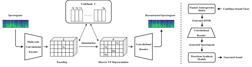
Fig. 1: Left: The proposed VQ-VAE based approach to learn a discrete T-F representation (DTFR) of sound. Right: The pipeline for conditional sound generation in the inference stage. We train the VQ-VAE model and the autoregressive model separately.

1 Introduction

General sounds carry a wide range of information about environments, from individual physical events to sound scenes as a whole [1]. General sound generation has many potential applications, such as the automatic production of sound effects for movies and video games [2]. In addition, due to the difficulties of collecting and annotating audio data, sound generation can be used as an efficient data augmentation [3] approach for acoustic scene classification [4] and sound event detection [5]. In the long term, sound search engines [6] could incorporate a sound generation system and customize sound according to the personal tastes of users.

Recently, significant progress has been made in speech synthesis [7, 8] and music generation [9, 10] using deep generative models. Compared with domain-specific sounds such as speech and music, general sound is less structured and has greater diversity, typically accompanied by noise and reverberation. Therefore, it is challenging to model general sounds using deep generative models. Related work on general sound generation includes acoustic scene generation [11] and environmental sound synthesis [12]. However, general sound generation remains a relatively unexplored area.

SampleRNN [13] is an autoregressive model for waveform generation, which has been adapted to sound generation by Kong et al. [11]. SampleRNN generates sound in the time domain and only back-propagates through a fraction of a second [14]. Thus, it is difficult to capture the long-range dependencies within sound clips using SampleRNN. However, some sound events typically have long-range dependencies, such as an ambulance siren spanning several seconds (tens of thousands of audio samples), and capturing these dependencies would be beneficial for the generation of such sounds.

Modeling sound in the time-frequency (T-F) domain, e.g. using spectrogram, can help capture long-range dependencies [14], although an additional step is required to convert the T-F representation into a time domain waveform. Recently, GAN-based methods [15, 16] have been proposed for waveform synthesis due to the computational efficiency offered by their parallel structure and good quality of synthesized audio. Synthesizing high-quality waveforms would normally require the spectrograms to be in high temporal resolution in order to retain the local and fine-grained characteristics that are important for sound fidelity. However, increasing the temporal resolution of the spectrogram (i.e., decreasing the short-time Fourier transform (STFT) hop size) would incur a higher computational cost.

In this paper, we propose an approach to generate sound conditioned on different sound classes in the T-F domain using a Vector Quantised Variational AutoEncoder (VQ-VAE) [17]. Our approach can model the long-range dependencies of sound while reducing the computational cost of modeling sound with high temporal resolution in the T-F domain. More specifically, a VQ-VAE model is trained to learn a discrete T-F representation (DTFR) of sound. Then, an improved autoregressive model [18] is trained using the DTFR as input and the sound classes as conditions to generate sounds. In addition, we propose a multi-scale convolutional scheme for the encoder of the VQ-VAE to capture acoustic information (i.e. features) of sound at different scales. We show that this leads to a compact DTFR while enables the encoding of local fine-grained structures of sound. To our knowledge, the VQ-VAE model has not yet been considered for the conditional generation of general sounds. We demonstrate empirically that our approach offers advantages in modeling the long-range dependencies of sound over the time-domain generation method [11].

We evaluate the diversity [11] and quality [19] (as described in Section 3.5) of the generated sound samples on the UrbanSound8K dataset [20]. Experimental results show that our proposed method outperforms the SampleRNN baseline [11] in diversity and has comparable performance in quality. The code and generated samples are available on GitHub.

2 Approach

To generate sound conditionally, we first use a VQ-VAE [17] to learn a DTFR of sound, as described in Section 2.1. Then, the process of generating sound using the DTFR conditioned on sound class labels is summarized in Section 2.2.

2.1 Discrete time-frequency representation learning

To disentangle the spectrogram representation of sound into a compressed DTFR, we employ a VQ-VAE-based model consisting of an encoder, a decoder and a codebook. Our proposed approach assumes fixed input size, the encoder learns a non-linear mapping from the spectrogram $x\in\mathbb{R}^{H\times W\times 1}$ onto a latent representation $z\in\mathbb{R}^{H/2^{m}\times W/2^{m}\times D}$ ($H$, $W$, $D$ are height, width and depth, respectively), where $m$ is a compression factor. The latent representation $z$ consists of $N$ elements $z_{n}\in\mathbb{R}^{1\times 1\times D}$, where $N=H/2^{m}\times W/2^{m}$. Each element ${z_{n}}$ is quantized based on its distance to the codewords $c_{k}$ in the codebook $C=\{c_{k}\}_{k=1}^{K}$ with $K$ being the number of codewords in the codebook $C$. Formally:

$$\operatorname{Quantize}(z_{n})=c_{k}\ \text{where}\ k=\mathop{\arg\min}_{i}\|z_{n}-c_{i}\|_{2},$$ (1)

where $z_{n}$ is reshaped to a vector of the same dimension as $c_{i}$ for calculation. After the quantization of each element in $z$, the DTFR defined as $r=\{r_{n}\}_{n=1}^{N}$ is obtained, and is fed into the decoder to reconstruct the spectrogram. The reconstructed spectrogram $\hat{x}$ is given by:

$$\hat{x}=\operatorname{Decoder}(r)=\operatorname{Decoder}(\operatorname{Quantize}(z)).$$ (2)

To learn the reconstruction process in Equation (2), the gradient is passed from the decoder input to the encoder output. The loss function of the VQ-VAE is defined as follows:

$$\mathrm{Loss}=\|x-\hat{x}\|_{2}^{2}\ +\ \|\text{sg}[z]-r\|_{2}^{2}+\ \beta\|\text{sg}[r]-z\|_{2}^{2},$$ (3)

where sg[·] denotes the stop-gradient operation [17], which ensures the operand is not updated during backpropagation, and $\beta$ is a regularization parameter. The first term is a reconstruction loss, the second term is used to align the codebook with the encoder output, and the last term is a commitment loss [17], which mitigates the uncertainty caused by noise in the mapping between the encoder output and the codewords.

2.1.1 Multi-scale convolutional scheme in the encoder

A conventional VQ-VAE uses a fully-convolutional encoder with a fixed kernel size, which can capture the local characteristics in the spectrograms but cannot make use of the dependencies between long-term temporal frames. To efficiently capture both local characteristics and long-range dependencies, we propose a multi-scale convolutional scheme in the encoder of the VQ-VAE. In this scheme, multi-scale CNNs with varied kernel sizes are deployed. This multi-scale convolutional approach has been shown to be effective in capturing the global and local information of audio signals in the T-F domain [21].

More precisely, the encoder consists of several strided convolutional layers (SCLs) in parallel. Each SCL has several consecutive sub-layers with strided convolutional kernels of fixed sizes followed by residual blocks. These SCLs have different kernel sizes. SCLs with small kernels are used to capture the local characteristics between the adjacent temporal frames, and SCLs with large kernels are utilized to explore the dependencies between long-range temporal frames. Then, the output of each SCL is added together to obtain the output of the encoder, thus enabling the encoder to capture global and local information (i.e. acoustic features) at different scales.

2.1.2 Model architecture

A fully-convolutional decoder is used to decode the DTFR to the reconstructed spectrogram. The structure of the decoder is similar to the encoder, except that the multi-scale convolutional scheme is omitted. The architecture of the proposed approach to learn the DTFR of sound is shown in Figure 1 (left). Details of the model will be discussed in Section 3.3.

2.2 Conditional sound generation

After learning the DTFR of sound, the task of conditional sound generation can be treated as generating the DTFR of sound, conditioned on the class labels. Since the DTFR is a compressed and compact representation, we can significantly alleviate the computational cost of modeling sound while still retaining the long-range dependencies and local characteristics of the sound. The decoder of the trained VQ-VAE model in Section 2.1.2 is used to map the generated DTFR to the generated spectrogram. The generation of the DTFR of a sound is described as below.

Considering that the index $k$ of the codewords $c_{k}$ can characterise the $n$th component of any DTFR $r=\{r_{n}\}_{n=1}^{N}$ (as described in Section 2.1), we first formulate $r$ as a sequence of indexes $y=\{y_{n}\}_{n=1}^{N}$ as follows:

$$y_{n}=k\ \ \text{where}\ \ r_{n}=c_{k}.$$ (4)

Then, we use an autoregressive model to build the distribution $p(y)$ over the DTFR of sound by factorising the joint distribution as a product of conditionals:

$$p(y)=p(y_{1},...,y_{n})=\prod_{i=1}^{n}p(y_{i}|y_{1},...,y_{i-1}).$$ (5)

To generate sound conditioned on a class label, we apply the one-hot encoding vector $h$ of a sound class as the global condition. Formally:

$$p(y|h)=p(y_{1},...,y_{n}|h)=\prod_{i=1}^{n}p(y_{i}|y_{1},...,y_{i-1},h).$$ (6)

We use PixelSNAIL [18] to build $p(y|h)$. PixelSNAIL is an improved autoregressive model that combines causal convolutions [22] with self-attention [23]. After training the VQ-VAE, we compute the DTFR of sound using the encoder of the trained VQ-VAE. Then PixelSNAIL is trained on the DTFR conditioned on class labels. The generation of the new DTFR is enabled by sampling the variables conditioned on all previous variables one by one from the trained autoregressive model. A waveform synthesis module, namely HiFi-GAN [16] (as described in Section 3.3.3), is deployed for converting the generated spectrogram into a waveform. The generation pipeline for our proposed approach in the inference stage is shown in Figure 1 (right).

3 Experiments

Table 1: Results of classification accuracy

	air_conditioner	car_horn	children_playing	dog_bark	drilling	engine_idling	gun_shot	jackhammer	siren	street_music	Average
Proposed Approach	0.8516	0.5049	0.1738	0.6875	0.9453	0.1875	0.7832	0.1240	0.6699	0.3613	0.5289
SampleRNN	0.6328	0.7119	0.7002	0.3438	0.3984	0.2305	0.4980	0.5840	0.6191	0.5625	0.5281
Test	0.4400	0.9375	0.9200	0.8500	0.6100	0.7640	0.9032	0.9146	0.9878	0.9700	0.8297
Reconstructed Test	0.3500	0.9688	0.8100	0.8700	0.8300	0.5843	0.8710	0.9024	0.9878	0.9000	0.8074

Table 2: Results of class-wise NDB and JSD

		air_conditioner	car_horn	children_playing	dog_bark	drilling	engine_idling	gun_shot	jackhammer	siren	street_music	Average
Proposed Approach	NDB${}_{\text{class}}$	6	4	4	2	3	1	1	3	4	3	3.1
	JSD${}_{\text{class}}$	0.0694	0.0522	0.0714	0.0351	0.0425	0.0336	0.0364	0.0357	0.0568	0.0448	0.0478
SampleRNN	NDB${}_{\text{class}}$	15	10	11	9	11	16	8	10	12	13	11.5
	JSD${}_{\text{class}}$	0.2897	0.1748	0.4859	0.3130	0.1632	0.3017	0.2856	0.1363	0.3251	0.2955	0.2771
Test	NDB${}_{\text{class}}$	1	1	1	0	0	2	0	1	2	0	0.8
	JSD${}_{\text{class}}$	0.2932	0.1881	0.1045	0.0427	0.0700	0.3476	0.2202	0.3677	0.2983	0.0964	0.2029

3.1 Dataset

We evaluate our proposed approach for conditional sound generation on the UrbanSound8K dataset [20]. UrbanSound8K consists of $8732$ labeled sound clips of urban sound from $10$ classes. The duration of each sound clip is less than $4$ seconds. UrbanSound8K has a large diversity of sound classes, such as siren and street music. In addition, each sound clip is divided into foreground sound or background sound. These attributes make it appropriate for using UrbanSound8K to evaluate the ability of the generative model to capture the salient features of different sound classes. UrbanSound8K is divided into $10$ folds and we use the predefined folds to obtain $7916$ sound clips for training and $816$ sound clips for testing. Because our proposed approach assumes that the length of input audio is fixed, we pad all sound clips to $4$ seconds. All sound clips are converted to $16\text{\,}\mathrm{b}\mathrm{i}\mathrm{t}$ and down-sampled to $22,050\text{\,}\mathrm{kHz}$.

3.2 Spectrogram computation

To generate high quality sound, we compute the spectrogram with the hyperparameter values as used in HiFi-GAN [16], which can achieve high-fidelity waveform synthesis, as described in Section 3.3.3. More precisely, we use an $80$-dimensional log mel-spectrogram calculated using the short-time Fourier transform (STFT) with a frame size of $1024$, a hop size of $256$, and a Hann window. Dynamic range compression is applied to the mel-spectrogram by first clipping it to a minimum value of $1\text{\times}{10}^{-5}$ and then applying a logarithmic transformation. A sound clip of 4 seconds results in a mel-spectrogram with shape $80\times 344$.

3.3 Details of model implementation

3.3.1 VQ-VAE

For the encoder of the VQ-VAE, we use four SCLs consisting of two sub-layers with stride $2$, followed by two $3\times 3$ residual blocks (ReLU, $3\times 3$ conv, ReLU, $1\times 1$ conv). The kernel sizes of these four SCLs are $2\times 2$, $4\times 4$, $6\times 6$ and $8\times 8$ respectively. Thus, we can down-sample the input log mel-spectrogram from $80\times 344$ to $20\times 86$ with compression factor $m=2$. The dimension of the codebook and each codeword are $512$ and $64$, respectively. The decoder has two $3\times 3$ residual blocks, followed by two transposed convolutional layers with stride $2$ and kernel size $4\times 4$. We train the VQ-VAE model using the Adam optimizer [24] with a learning rate of $3\text{\times}{10}^{-4}$ and a batch size of $64$ for $70,000$ iterations.

3.3.2 Autoregressive model

The PixelSNAIL [18] model is trained on the $20\times 86$ DTFR of sound using the Adam optimizer [24] with a learning rate of $3\text{\times}{10}^{-4}$ and a batch size of $32$ for $250,000$ iterations. We use a PyTorch implementation of PixelSNAIL.

3.3.3 Waveform synthesis module

The generated mel-spectrograms are converted into waveforms using HiFi-GAN [16], which provides high-fidelity speech synthesis results and fast inference. We train a HiFi-GAN on the training data of UrbanSound8K dataset from scratch using the code provided in the official GitHub repository.

3.4 Baseline system

SampleRNN has been adapted for sound generation in [11]. In this work, we use a two-tier conditional SampleRNN as the baseline system. The baseline system is trained on raw waveforms for $350,000$ iterations using the Adam optimizer [24] with a learning rate of $1\text{\times}{10}^{-3}$ and a batch size of $64$.

3.5 Evaluation methods

Several subjective metrics [25] have been proposed for evaluating the performance of acoustic generative models. However, a subjective evaluation of sound is time-consuming and the results are sometimes difficult to reproduce. In this work, we adopt the quality and diversity of generated sound samples as two objective performance metrics.

3.5.1 Generation quality

Similar to the evaluation metric used in [11], we train a VGG11 [26] classifier on the training data and then use the trained VGG11 to classify the generated data. If the generated data is of high quality, the VGG11 will assign them to the corresponding sound classes with high accuracy. If the generated data is of low quality, such as random noise, the VGG11 will tend to predict them as random classes. Although this metric does not indicate the perceptual quality of the generated sound, it is still useful for partially assessing how good the generated sound is. The VGG11 classifier is trained on the computed spectrogram (mentioned in Section 3.2) of training data using the Adam optimization algorithm [24] with a batch size of $128$ and a learning rate of $5\text{\times}{10}^{-4}$. The VGG11 classifier achieves a $83$% accuracy on testing data after training for $3100$ iterations.

3.5.2 Generation diversity

The number of statistically-different bins (NDB) [19] has been proposed to evaluate generative models. This evaluation metric first clusters the training data into different bins and then assigns each generated data to the nearest bin. NDB is reported as the number of bins where the number of training instances is statistically different from the number of generated instances by a two-sample Binomial test. In addition, the Jensen-Shannon divergence (JSD) between the distribution of the training data and generated data over the clustered bins is calculated as the evaluation metric if the number of samples is sufficiently large. A smaller NDB and JSD represent better performance. We adopt the K-means algorithm to cluster sound data in the T-F domain (as reported in Section 3.2). We then calculate the NDB and JSD of the generated sound in the class-wise case and the all-classes case (merge the generated data of all classes together and compare with the training data), respectively. $20$ bins are used for class-wise clustering and $200$ bins are used for all-classes clustering. We use the official implementation of NDB and JSD.

3.6 Evaluation results

We use our proposed method and the baseline to generate $1024$ sound clips per class. Evaluation results are discussed below.

3.6.1 Generation quality

Table 1 shows a VGG11 classification accuracy of $52.89$%, $52.81$%, $82.97$%, $80.74$% on the data generated by our proposed approach (Proposed Approach), data generated by baseline (SampleRNN), testing data (Test), and testing data after the reconstruction based on DTFR (Reconstructed Test), respectively. Our proposed approach achieves a comparable performance in generation quality compared with SampleRNN. Sound classes such as dog bark and gunshot perform better, while sound classes such as jackhammer and children playing perform worse. In addition, although the DTFR is four times smaller than the spectrogram, the classification accuracy on the testing data after reconstruction only decreases by $2.23$ percentage points, which confirms the effectiveness of DTFR.

3.6.2 Generation diversity

The results of class-wise and all-classes evaluations of generation diversity are shown in Table 2 and Table 3, respectively. Our proposed approach outperforms the SampleRNN baseline significantly in NDB and JSD for all sound classes, which means the data generated by our approach has greater diversity and its distribution is closer to the real data. The JSD of the testing data is higher than the data generated by our proposed approach because the size of the testing data is small and the class distribution is different from the training data.

Table 3: Results of all-classes NDB and JSD

	NDB${}_{\text{all-classes}}$	JSD${}_{\text{all-classes}}$
Proposed Approach	25	0.0461
SampleRNN	120	0.3267
Test	6	0.1359

3.7 Ablation study

We investigate the impact of the multi-scale convolutional scheme (MSCS) in the VQ-VAE’s encoder. Table 4 shows the mean square error (MSE) and the VGG11 classification accuracy of the reconstructed test data based on DTFR with and without MSCS. Experimental results show that by applying the MSCS, the MSE decreases by $0.0047$ and the VGG11 classification accuracy increases by $6.2$ percentage points, which indicates that more acoustic information (i.e. local fine-grained structures) within sound is captured by MSCS.

4 Conclusions

We have presented a novel approach for conditional sound generation using neural discrete time-frequency representation learning. Our proposed approach can efficiently model long-range dependencies and retrain local fine-grained structures within sound clips. Experimental results show that our proposed method has better performance in diversity and has comparable performance in quality compared to SampleRNN. In future work, we will consider learning a representation via adversarial training [27] and perceptual loss [28], and compare it with other GAN-based audio generative model [29].

Table 4: Results of ablation experiment

	MSE	Accuracy
DTFR w/   MSCS	0.0684	0.8074
DTFR w/o MSCS	0.0731	0.7454

References

- [1] T. Virtanen, M. D. Plumbley, and D. Ellis, “Introduction to sound scene and event analysis,” in Computational Analysis of Sound Scenes and Events, 1st ed. Springer, 2018.
- [2] D. B. Lloyd, N. Raghuvanshi, and N. K. Govindaraju, “Sound synthesis for impact sounds in video games,” in Symposium on Interactive 3D Graphics and Games, 2011, pp. 55–62.
- [3] J. Salamon, D. MacConnell, M. Cartwright, P. Li, and J. P. Bello, “Scaper: A library for soundscape synthesis and augmentation,” in 2017 IEEE Workshop on Applications of Signal Processing to Audio and Acoustics (WASPAA), 2017, pp. 344–348.
- [4] Z. Ren, K. Qian, Z. Zhang, V. Pandit, A. Baird, and B. Schuller, “Deep scalogram representations for acoustic scene classification,” IEEE/CAA Journal of Automatica Sinica, vol. 5, no. 3, pp. 662–669, Apr. 2018.
- [5] Q. Kong, Y. Xu, W. Wang, and M. D. Plumbley, “Sound event detection of weakly labelled data with CNN-transformer and automatic threshold optimization,” IEEE/ACM Transactions on Audio, Speech, and Language Processing, vol. 28, pp. 2450–2460, Aug. 2020.
- [6] V. Akkermans, F. Font Corbera, J. Funollet, B. De Jong, G. Roma Trepat, S. Togias, and X. Serra, “Freesound 2: An improved platform for sharing audio clips,” in Proceedings of the 12th International Society for Music Information Retrieval Conference (ISMIR), 2011.
- [7] J. Shen, R. Pang, R. J. Weiss, M. Schuster, N. Jaitly, Z. Yang, Z. Chen, Y. Zhang, Y. Wang, R. Skerrv-Ryan et al., “Natural TTS synthesis by conditioning WaveNet on mel spectrogram predictions,” in IEEE International Conference on Acoustics, Speech and Signal Processing (ICASSP), 2018, pp. 4779–4783.
- [8] Y. Wang, R. Skerry-Ryan, D. Stanton, Y. Wu, R. J. Weiss, N. Jaitly, Z. Yang, Y. Xiao, Z. Chen, S. Bengio, Q. V. Le, Y. Agiomyrgiannakis, R. Clark, and R. A. Saurous, “Tacotron: Towards end-to-end speech synthesis,” in Proceedings of Interspeech, 2017.
- [9] L.-C. Yang, S.-Y. Chou, and Y.-H. Yang, “MidiNet: A convolutional generative adversarial network for symbolic-domain music generation,” in Proceedings of the 18th International Society for Music Information Retrieval (ISMIR), 2017.
- [10] S. Dieleman, A. V. D. Oord, and K. Simonyan, “The challenge of realistic music generation: modelling raw audio at scale,” Advances in Neural Information Processing Systems (NIPS) 31, pp. 8000–8010, 2018.
- [11] Q. Kong, Y. Xu, T. Iqbal, Y. Cao, W. Wang, and M. D. Plumbley, “Acoustic scene generation with conditional SampleRNN,” in IEEE International Conference on Acoustics, Speech and Signal Processing (ICASSP), 2019, pp. 925–929.
- [12] Y. Okamoto, K. Imoto, S. Takamichi, R. Yamanishi, T. Fukumori, and Y. Yamashita, “Onoma-to-wave: Environmental sound synthesis from onomatopoeic words,” arXiv preprint arXiv:2102.05872, 2021.
- [13] S. Mehri, K. Kumar, I. Gulrajani, R. Kumar, S. Jain, J. Sotelo, A. Courville, and Y. Bengio, “SampleRNN: An unconditional end-to-end neural audio generation model,” 5th International Conference on Learning Representations (ICLR), 2017.
- [14] S. Vasquez and M. Lewis, “MelNet: A generative model for audio in the frequency domain,” arXiv preprint arXiv:1906.01083, 2019.
- [15] K. Kumar, R. Kumar, T. de Boissiere, L. Gestin, W. Z. Teoh, J. Sotelo, A. de Brébisson, Y. Bengio, and A. Courville, “MelGAN: Generative adversarial networks for conditional waveform synthesis,” Advances in Neural Information Processing Systems (NIPS) 32, 2019.
- [16] J. Kong, J. Kim, and J. Bae, “HiFi-GAN: Generative adversarial networks for efficient and high fidelity speech synthesis,” Advances in Neural Information Processing Systems (NIPS) 33, 2020.
- [17] A. V. D. Oord, O. Vinyals, and K. Kavukcuoglu, “Neural discrete representation learning,” Advances in Neural Information Processing Systems (NIPS) 30, pp. 6306–6315, 2017.
- [18] X. Chen, N. Mishra, M. Rohaninejad, and P. Abbeel, “PixelSNAIL: An improved autoregressive generative model,” in International Conference on Machine Learning (ICML), 2018, pp. 864–872.
- [19] E. Richardson and Y. Weiss, “On GANs and GMMs,” Advances in Neural Information Processing Systems (NIPS) 31, 2018.
- [20] J. Salamon, C. Jacoby, and J. P. Bello, “A dataset and taxonomy for urban sound research,” in Proceedings of the 22nd ACM International Conference on Multimedia, 2014, pp. 1041–1044.
- [21] Y. Xian, Y. Sun, W. Wang, and S. M. Naqvi, “Multi-scale residual convolutional encoder decoder with bidirectional long short-term memory for single channel speech enhancement,” in 28th European Signal Processing Conference (EUSIPCO), 2021, pp. 431–435.
- [22] A. V. D. Oord, N. Kalchbrenner, O. Vinyals, L. Espeholt, A. Graves, and K. Kavukcuoglu, “Conditional image generation with PixelCNN decoders,” Advances in Neural Information Processing Systems (NIPS) 29, 2016.
- [23] A. Vaswani, N. Shazeer, N. Parmar, J. Uszkoreit, L. Jones, A. N. Gomez, L. Kaiser, and I. Polosukhin, “Attention is all you need,” Advances in Neural Information Processing Systems (NIPS) 30, 2017.
- [24] D. P. Kingma and J. Ba, “Adam: A method for stochastic optimization,” 3rd International Conference on Learning Representations (ICLR), 2015.
- [25] Y. Okamoto, K. Imoto, T. Komatsu, S. Takamichi, T. Yagyu, R. Yamanishi, and Y. Yamashita, “Overview of tasks and investigation of subjective evaluation methods in environmental sound synthesis and conversion,” arXiv preprint arXiv:1908.10055, 2019.
- [26] T. Iqbal, Q. Kong, M. D. Plumbley, and W. Wang, “General-purpose audio tagging from noisy labels using convolutional neural networks,” in Proceedings of the Detection and Classification of Acoustic Scenes and Events, 2018, pp. 212–216.
- [27] A. Makhzani, J. Shlens, N. Jaitly, I. Goodfellow, and B. Frey, “Adversarial autoencoders,” arXiv preprint arXiv:1511.05644, 2015.
- [28] Q. Liu, W. Wang, P. J. Jackson, and Y. Tang, “A perceptually-weighted deep neural network for monaural speech enhancement in various background noise conditions,” in 25th European Signal Processing Conference (EUSIPCO), 2017, pp. 1270–1274.
- [29] C. Donahue, J. McAuley, and M. Puckette, “Adversarial audio synthesis,” 7th International Conference on Learning Representations (ICLR), 2019.