Singlet channel scattering in a Composite Higgs model on the lattice

Abstract

We present the first calculation of the scattering amplitude in the singlet channel beyond QCD. The calculation is performed in $SU(2)$ gauge theory with $N_{f}=2$ fundamental Dirac fermions and based on a finite-volume scattering formalism. The theory exhibits a $SU(4)\to Sp(4)$ chiral symmetry breaking pattern that is used to design minimal composite Higgs models currently tested at the LHC. Our results show that, for the range of underlying fermion mass considered, the lowest flavour singlet state is stable.

I Introduction

The discovery of the Standard Model’s (SM) last missing piece, the Higgs boson, and the increase in precision of tests of its properties, continue to trigger the study of numerous mechanisms to address the fundamental problems with its formulation.

Among other possibilities, a new strongly interacting sector giving rise to the observed phenomenology at the electroweak scale (EW) and below has been pursued for decades. Such a new sector could feature a solution to the naturalness problem and provide a mechanism to generate a non-trivial mass spectrum together with a large scale separation. These mechanisms have been used for instance in the context of Composite Higgs models Terazawa et al. (1977); Terazawa (1980); Kaplan and Georgi (1984); Kaplan et al. (1984); Dugan et al. (1985); Bardeen et al. (1986); Leung et al. (1986); Yamawaki et al. (1986), of scenarios of dynamical electroweak symmetry breaking Weinberg (1976); Susskind (1979), and of Dark Matter models Hochberg et al. (2014); Tsai et al. (2020). These appealing ideas motivate the lattice endeavour to understand gauge theories beyond QCD.

One feature of a strongly interacting sector is the inevitable presence of a flavour singlet state of positive parity—referred to as $\sigma$ in the rest of this paper. In QCD-like theories, the $\sigma$ is expected to be a resonance of two Goldstone bosons in the limit of massless underlying fermions.

In Composite Higgs scenarios, the embedding of the new strong sector in the Standard Model is such that the Goldstone bosons of the strong sector play the role of the SM Higgs field. In these models, aside from the Goldstone bosons, also the presence of new resonances like the $\sigma$ can affect the predictions for the LHC Contino et al. (2011), and could be detected by the next generation of colliders Bharucha et al. (2021). In general, the phenomenological implications of the new scalar resonance in a composite Higgs scenario will depend on the underlying dynamics and on the details of the electroweak embedding. Unless the model features a parametrically large scale separation between the Goldstone bosons and the $\sigma$, the effective description at the EW scale must take the $\sigma$ into account. The mixing of the scalar $\sigma$ resonance with the Goldstone bosons associated with the spontaneous symmetry breaking of the new strong sector is induced by the interaction with the SM, and gives rise to an additional effective scalar field with a larger mass, see Refs. Bellazzini et al. (2016); Bizot et al. (2017); Niehoff et al. (2017). Such a resonance is expected to be produced at the LHC similarly to the SM Higgs, i.e. via gluon fusion and vector boson fusion mechanisms, as discussed for instance in Ref. Buarque Franzosi et al. (2020). Effective theories at the EW scale will encode the actual realisation of the Composite Higgs scenarios through their low energy constants, under the assumption of a strong sector weakly coupled to the Standard Model. Given the large number of low energy couplings parametrising the effective Lagrangian, additional theoretical constraints are needed to discriminate among Composite Higgs models. Lattice calculations can reduce the space of parameters by performing measurements on the new strong sector in isolation. The present work contributes to our understanding of the role of the $\sigma$ resonance in the phenomenology of the class of composite models characterised by the strong sector we are considering, irrespectively of its embedding.

In lattice simulations the only rigorous approach to reveal the nature of a resonance is to estimate the scattering amplitude of the Goldstone bosons. Lattice simulations in various gauge theories have estimated the mass of the $\sigma$ in a regime where it is stable Aoki et al. (2013, 2014); Fodor et al. (2015); Brower et al. (2016); Arthur et al. (2016a); Hasenfratz et al. (2017); Appelquist et al. (2016); Athenodorou et al. (2017); Appelquist et al. (2019); Lee et al. (2018); Bennett et al. (2019). Scattering amplitudes have been evaluated also for other channels, see for instance the recent work in a possible nearly conformal theory for $SU(3)$ with $N_{f}=8$ flavours in the maximal-isospin channel Appelquist et al. (2021) and our recent work in the vector meson channel for $SU(2)$ with $N_{f}=2$ flavours Drach et al. (2021).

In this work, we consider an $SU(2)$ gauge theory with $N_{f}=2$ fundamental Dirac fermions. The theory features an extended $SU(4)$ flavour symmetry that spontaneously breaks to $Sp(4)$. The theory is used to build a pseudo-Nambu–Goldstone boson (PNGB) Composite Higgs model in Ref. Cacciapaglia and Sannino (2014), and it was recently reviewed in Ref. Cacciapaglia et al. (2020). In this model, the physical Higgs boson is a mixture of PNGBs and of the flavour singlet state of the strong sector. The model has been shown to pass experimental constraints Cacciapaglia et al. (2020), and the mixing between the scalar resonance and the Higgs can relax the bounds on the model Buarque Franzosi et al. (2020).

We present here the first calculation of the scattering amplitude of Goldstone bosons in the flavour singlet channel beyond QCD. We have used two operators to constrain the scattering amplitude at two different kinematic configurations. The evaluation of disconnected contributions increases significantly the computational cost with respect to other channels.

We also report on the comparison of our results to the chiral perturbation theory predictions (in isolation of the SM) of Ref. Bijnens and Lu (2011), which should match in the limit of light enough PNGBs.

II Lattice setup

We use the HiRep Del Debbio et al. (2010) suite to simulate an $SU(2)$ gauge theory with $N_{f}=2$. For the fundamental fermions the action of choice is the Wilson action Wilson (1974) with tree-level $O(a)$-improvement clover term Sheikholeslami and Wohlert (1985). For the gauge we use the tree-level Symanzik improved action Lüscher and Weisz (1985). Both the bare mass term, $a\,m_{0}$, and the Wilson term explicitly break the $SU(4)$ flavour symmetry to an $Sp(4)$ subgroup. All of our simulation are performed with periodic boundary conditions in all space-time directions, both in gauge and fermion fields.

Ensemble	$L/a$	$T/a$	$\beta$	$a\,m_{0}$	$c_{sw}$	# configs
Heavy	24	48	1.45	$-0.6050$	1.0	1980
Light	32	48	1.45	$-0.6077$	1.0	1160

Table 1: Simulation parameters in our ensembles.

The ensembles used for this work have been generated for $\beta=1.45$, and two different values of the bare fermion mass. We refer to these ensembles as “light” and “heavy” depending on the value of the pion mass. Here and in the following, we will make use of the naming convention inherited from QCD, that is, the pseudoscalar PNGB of this theory is referred to as pion. The spatial size of the ensembles has been tuned to obtain a value of $M_{\pi}L\simeq 5$. All the relevant simulation parameters are given in Table 1.

For each ensemble, we compute the PNGB mass, $M_{\pi}$, and the vector mass, $M_{\rho}$ from the Euclidean time dependence of appropriate correlation functions. We also extract the bare pseudoscalar decay constant $F_{\pi}^{\rm{bare}}$, which renormalises multiplicatively with the renormalization factor $Z_{A}$. For more details about the calculation of these quantities, we refer the reader to Ref. Arthur et al. (2016b). All our findings are summarised in Table 2.

In addition, the non-perturbative determination of $Z_{A}$ was carried out using the RI’-MOM scheme Martinelli et al. (1995), using the same strategy as in the previous setup Arthur et al. (2016b). For detailed information about the $Z_{A}$ determination we refer to Ref. Drach et al. (2021), where we estimated $Z_{A}=0.8022(3)$ for the same value of $\beta$ used in this work.

Ensemble	$aM_{\pi}$	$aM_{\rho}$	$aF_{\pi}^{\text{bare}}$	$M_{\pi}/F_{\pi}^{\text{bare}}$
Heavy	0.2065(12)	0.438(27)	0.0395(9)	5.24(11)
Light	0.1597(18)	0.3864(30)	0.0357(9)	4.36(11)

Table 2: Pion mass, vector mass and decay constant for our two ensembles.

III Scattering in $\boldsymbol{SU(2)}$

In this section we will review and extend the necessary theoretical background for this work. In particular, we will derive all the group classification needed to evaluate the operators and the associated correlation functions for the singlet channel, as well as the finite-volume scattering formalism and the effective field theory (EFT) description of the relevant scattering amplitude.

III.1 Flavour singlet operators

We start by considering the flavour symmetries of the $SU(2)$ gauge theory with $N_{f}=2$. It can be shown that the massless Lagrangian is symmetric under an $SU(4)$ flavour transformation, while the mass term can be shown to be $Sp(4)$ invariant. This means that there exist five broken generators, which correspond to the pseudo-Nambu–Goldstone fields. More specifically, it can be shown that they correspond to the three pions and two dibaryons. In terms of the two fundamental fermion fields $u$ and $d$, we can construct one-particle operators with the right quantum numbers as follows:

$$\Pi_{ud}(x) =u^{T}(x)(-i\sigma_{2})C\gamma_{5}d(x),$$

$$\Pi_{\bar{u}\bar{d}}(x) =\bar{u}(x)(-i\sigma_{2})C\gamma_{5}\bar{d}(x)^{T},$$

$$\pi^{-}(x) =\bar{u}(x)\gamma_{5}d(x),$$ (1)

$$\pi^{+}(x) =-\bar{d}(x)\gamma_{5}u(x),$$

$$\pi^{0}(x) =\frac{1}{\sqrt{2}}\left[\bar{u}(x)\gamma_{5}u(x)-\bar{d}(x)\gamma_{5}d(x)\right],$$

where $x\equiv({\bf x},t)$. The real and antisymmetric matrix ($-i\sigma_{2}$) acts in colour space, and $C$ represents the conjugation charge matrix, $C=i\gamma_{0}\gamma_{2}$. As we are interested only in the flavour structure of the operators, we will omit the space-time dependence of the fields in the equations where possible.

In order to build a flavour singlet operator, we introduce:

$$\begin{split}Q=\begin{pmatrix}u_{L}\\ d_{L}\\ \widetilde{u}_{L}\\ \widetilde{d}_{L}\\ \end{pmatrix}&=\begin{pmatrix}u_{L}\\ d_{L}\\ (-i\sigma_{2})C\bar{u}^{T}_{R}\\ (-i\sigma_{2})C\bar{d}^{T}_{R}\\ \end{pmatrix},\\ \quad E&=\begin{pmatrix}0&\mathbbm{1}_{2}\\ -\mathbbm{1}_{2}&0\end{pmatrix}\,,\end{split}$$ (2)

where we are using the convention from Ref.Ryttov and Sannino (2008), summarised in appendix A, together with the standard definition of $q_{L,R}=P_{L,R}\,q$ and $\bar{q}_{L,R}=\bar{q}\,P_{R,L}$ where $P_{L}={(1-\gamma_{5})}/{2}$ and $P_{R}={(1+\gamma_{5})}/{2}$.

With the above convention we can define the multiplet $\Pi^{i=1,\dots,5}$ and the singlet $\mathcal{O}_{\sigma}$ as

$$\begin{split}\Pi^{i}&=\frac{1}{2}\left[Q^{T}(-i\sigma_{2})C\gamma_{5}X^{i}EQ+\textrm{h.c}\right]\ ,\\ \qquad{\mathcal{O}_{\sigma}}&=\frac{1}{\sqrt{2}}\left[Q^{T}(-i\sigma_{2})CEQ+\textrm{h.c}\right].\end{split}$$ (3)

Here $X^{i=1,\dots,5}$ are the broken generators used to parametrise the coset $SU(4)/Sp(4)$ defined in the appendix.

Considering the infinitesimal transformation

$$Q\longrightarrow\left(\mathbbm{1}_{4}+i\alpha^{a}S^{a}\right)Q,$$ (4)

where $\alpha^{i=1,\dots,10}$ are real parameters, and $S^{a=1,\dots,10}$ are the generators of the Lie Algebra of $Sp(4)$. The generators obey the Lie algebra defining relation:

$$ES^{a}+(S^{a})^{T}E=0.$$ (5)

It is straightforward to show that $\mathcal{O}_{\sigma}$ is a singlet of $Sp(4)$. It can also be shown by performing explicitly an infinitesimal transformation that the multiplet ${\Pi}$ transforms as a 5-dimensional irreducible representation of $Sp(4)$ and that any operator proportional to ${\mathrm{tr}\left[\Pi\otimes\Pi\right]}$ is a singlet of $Sp(4)$. The reader interested in more details is referred to Appendix B.
The operator

$$\mathcal{O}_{\pi\pi}=-\frac{4}{\sqrt{5}}\sum_{i=1}^{5}\Pi^{i}\Pi^{i}$$ (6)

is therefore a flavour singlet operator. Expressing the operator $\mathcal{O}_{\pi\pi}$ in terms of the bilinear defined in Eq. III.1, we find:

$$\begin{split}\mathcal{O}_{\pi\pi}=\frac{1}{\sqrt{5}}\Big{[}&+\pi^{+}\pi^{-}+\pi^{-}\pi^{+}-\pi^{0}\pi^{0}\\ &+\Pi_{ud}\Pi_{\bar{u}\bar{d}}+\Pi_{\bar{u}\bar{d}}\Pi_{ud}\Big{]}.\end{split}$$ (7)

Similarly the operator $\mathcal{O}_{\sigma}$ can be expressed in terms of the $u$ and $d$ fields as:

$$\mathcal{O}_{\sigma}=\frac{1}{\sqrt{2}}\left[\bar{u}(x)u(x)+\bar{d}(x)d(x)\right].$$ (8)

In the following, we will use $\mathcal{O}_{\pi\pi}$ and $\mathcal{O}_{\sigma}$ as the relevant operators to study the singlet channel. We refer to them respectively as the two-pion and sigma operators.

III.2 Contractions

Figure 1: Representation of the different contractions needed for this work. The blobs indicate a fermion bilinear, with gamma matrix $\gamma_{5}$ or identity. The physical correlation functions are constructed from linear combinations thereof as given in Eq. 13.

In the rest of the paper we will use the zero momentum projection of the operators defined in Eq. III.1 for the evaluation of the correlators. Explicitly, this is given by

$$\Pi_{ud}(t) =\sum_{\bf x}\Pi_{ud}({\bf x},t),$$ (9)

and analogously for the other one-particle operators.

The energy of the flavour singlet state can be computed from the exponential decay in time of the appropriate correlation functions of the two-pion and sigma operators described in the previous section.

The singlet two-pion operator, with each one-particle operator projected at zero momentum is

$$\begin{split}\mathcal{O}_{\pi\pi}(t)&=\frac{1}{\sqrt{5}}\bigg{[}\pi^{+}(t)\pi^{-}(t)+\pi^{-}(t)\pi^{+}(t)\\ &-\pi^{0}(t)\pi^{0}(t)\\ &+\Pi_{ud}(t)\Pi_{\bar{u}\bar{d}}(t)+\Pi_{\bar{u}\bar{d}}(t)\Pi_{ud}(t)\bigg{]},\end{split}$$ (10)

where we have included the Euclidean time explicitly. Analogously, the zero momentum projected sigma operator can be rewritten as

$$\mathcal{O}_{\sigma}(t)=\frac{1}{\sqrt{2}}\sum_{\bf x}\left(\bar{u}({\bf x},t)u({\bf x},t)+\bar{d}({\bf x},t)d({\bf x},t)\right).$$ (11)

Using the two operators in Eqs. 10 and 11, we can build a symmetric two-by-two matrix of correlation functions as follows:

$$C_{X\to Y}(\delta t)=\frac{1}{T}\sum_{t}\langle O_{X}(t+\delta t)O_{Y}(t)^{\dagger}\rangle.$$ (12)

By solving the associated generalised eigenvalue problem (GEVP) Lüscher and Wolff (1990), we are able to obtain the energy of the two lowest states in the spectrum, by measuring the exponential decay of the two eigenvalues.

The three different correlation functions that enter in Eq. 12 can be built from eight different Wick contractions:

$$\begin{split}C_{\sigma\to\sigma}(t)&=-B(t)+2\Sigma(t),\\ C_{\pi\pi\to\pi\pi}(t)&=2D(t)+3X(t)-10R(t)+5V(t),\\ C_{\pi\pi\to\sigma}(t)&=\sqrt{10}\left(T(t)-W(t)\right).\end{split}$$ (13)

These are defined in Fig. 1, along with their naming conventions. Three of the contractions include disconnected diagrams: $V$, $W$ and $\Sigma$, and, as will be seen later, they dominate the statistical uncertainty.

III.3 Extraction of scattering amplitudes

The Lüscher method Lüscher (1986a, 1991a, 1991b) provides a way to obtain two-particle scattering amplitudes from lattice simulations. The so-called quantization condition connects the finite-volume energy levels to the phase shift. It is a well-established technique Rummukainen and Gottlieb (1995); Kim et al. (2005); He et al. (2005); Bernard et al. (2011); Briceño and Davoudi (2013); Briceño (2014); Romero-López et al. (2018); Luu and Savage (2011); Göckeler et al. (2012), which has been applied to many systems—see Ref. Briceño et al. (2018a) for a review. In the context of QCD the singlet channel has often been studied, see for example Refs. Guo et al. (2018); Fu and Chen (2018); Mai et al. (2019); Briceno et al. (2017); Briceño et al. (2018b); Liu et al. (2017).

In the case of two identical scalars with only $s$-wave interactions, the quantization condition reads Lüscher (1986a):

$$k\cot\delta_{0}\left(k\right)=\frac{2}{\sqrt{\pi}L}\mathcal{Z}_{00}(\eta^{2}),\quad\eta=\frac{Lk}{2\pi},$$ (14)

where the energy levels are in the $A_{1}^{+}$ irreducible representation of the octahedral group, and $k$ is the relative momentum in the center-of-mass (CM) frame. Furthermore, $\mathcal{Z}_{00}$ is the standard Lüscher zeta function. Note that in this form, the quantization condition is a one-to-one mapping between an energy level and a point in the phase shift curve.

It is convenient, for our discussion later, to highlight how bound states manifest themselves in the phase shift both at finite and infinite volume.

In infinite volume, they correspond to poles in the scattering amplitude. The pole’s position is given by

$$k\cot\delta_{0}\left(k\right)=-\sqrt{-k^{2}},$$ (15)

which we denote as bound-state condition. The fact that the residue of the pole has a positive sign, implies the following condition Iritani et al. (2017):

$$\frac{d}{dk^{2}}\left[\ k\cot\delta_{0}\left(k\right)-\left(-\sqrt{-k^{2}}\right)\ \right]<0.$$ (16)

This means that $k\cot\delta_{0}$ must cross the bound-state condition from below with decreasing $k^{2}$.

By contrast, the finite-volume solutions to the quantization condition never intersect the bound-state condition. They are however exponentially close Lüscher (1986b), with an exponent related to the binding momentum König and Lee (2018).

III.4 EFT prediction

At sufficiently low energies and close to the chiral limit, Chiral Perturbation Theory (ChPT) should provide a satisfactory description of the interactions of Goldstone bosons in QCD-like theories. However, the precise predictions depend upon the symmetry breaking pattern. As explained before, in our case an $SU(4)$ flavour symmetry is spontaneously broken down to $Sp(4)$. This was worked out in Refs. Bijnens and Lu (2009, 2011), and is referred to as the pseudo-real case.

In the present work the quantity of interest is the two-pion scattering amplitude in the singlet channel—analogous to that of the “$\sigma$” resonance in QCD. In this exploratory study, the leading-order (LO) ChPT result will suffice. This reads

$$\mathcal{T}_{I}=\frac{M_{\pi}^{2}}{F_{\pi}^{2}}\left(-\frac{3}{2}+2\frac{s}{M_{\pi}^{2}}\right),$$ (17)

where we are using the convention $f_{\pi}=\sqrt{2}F_{\pi}$ for the normalization of the decay constant, and $\sqrt{s}$ is the CM energy. From the scattering amplitude, the momentum dependence of the phase-shift can be easily derived:

$$\text{Re }\frac{1}{\mathcal{T}_{I}}=\frac{k\cot\delta^{I}_{0}}{16\pi\sqrt{s}}.$$ (18)

The LO result is

$$\frac{k}{M_{\pi}}\cot\delta^{I}_{0}=\frac{M_{\pi}\sqrt{s}}{13M_{\pi}^{2}+16k^{2}}\left(\frac{32\pi F_{\pi}^{2}}{M_{\pi}^{2}}\right).$$ (19)

Furthermore, the scattering length is defined as

$$\lim_{k\to 0}\frac{k}{M_{\pi}}\cot\delta^{I}_{0}=-\frac{1}{M_{\pi}a^{I}_{0}},$$ (20)

and its result reads

$$M_{\pi}a_{0}^{I}=-\frac{13}{64\pi}\frac{M_{\pi}^{2}}{F_{\pi}^{2}}.$$ (21)

An interesting remark is that the leading-order amplitude has a zero below threshold (Adler zero), which translates to a pole in $k\cot\delta_{0}^{I}$. This is located at $(k/M_{\pi})^{2}=-13/16$, and may limit the converge of a polynomial expansion of $k\cot\delta_{0}^{I}$ in $k^{2}$—the so-called threshold expansion. Such behaviour has been observed, e.g., in the isospin-2 $\pi\pi$ system in QCD Blanton et al. (2020).

IV Results

IV.1 Correlation functions

We construct the correlation functions as indicated in Eq. 13. In order to evaluate all the contractions depicted in Fig. 1, we use various types of stochastic sources. First, for the $D,X,R,V$ and $B$ contractions we use time-diluted stochastic sources. By placing a source in each of the timeslices, we can obtain a single stochastic estimator for each of these contractions. In this case we use $10$ stochastic estimators, which require $T\times 10$ inversions of sources. By contrast, we use $40$ volume sources for the $\Sigma$ contraction, while for $W$ we combine the building blocks of $V$ and $\Sigma$. Finally, $T$ is computed by employing $40$ time-diluted sources that have an additional sequential inversion.

The contractions $\Sigma$ and $W$ are responsible for the largest contribution to the statistical uncertainty. This is because they contain the trace of a single propagator multiplied by the identity in spinor space, and so, they are dominated by the gauge noise. Because of this, we choose to measure them more often than the other building blocks. In fact, we measure the trace of the single propagator in steps of one unit of Monte Carlo time.

We perform the analysis of uncertainties using jackknife samples. In order to account for autocorrelations, we use the binning procedure. For this, we average correlation functions within a bin length of $10$ units of Monte Carlo time. We have checked that larger bin sizes, 20 and 30, do not lead to any substantial change in the estimation of uncertainties.

As the operators have vacuum quantum numbers, there is an overall constant in all our correlation functions. Because of this, we will work with the shifted correlator:

$$\widetilde{C}(t)=\frac{1}{2}\big{[}C(t-1)-C(t+1)\big{]}.$$ (22)

This is a discrete version of the derivative in Euclidean time that keeps the same exponential decay, but cancels the undesired constant.

The results for the two ensembles are shown in Fig. 2. As can be seen, the statistical noise is dominated by the ones including the $\mathcal{O}_{\sigma}$ operator, which contain the $W$ and $\Sigma$ contractions in Fig. 1. It is also clear that one cannot trust the correlator in the region dominated by the statistical noise.

(a) Ensemble with heavier pion mass.

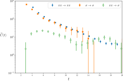
(b) Ensemble with lighter pion mass.

Figure 2: Correlation functions built with two different operators with singlet quantum numbers. For visualization purposes we include an arbitrary normalization.

IV.2 Spectrum determination

We now turn to the determination of the spectrum. For this, we build a two-by-two matrix, as presented in Eq. 12. The GEVP is defined by means of the shifted correlator as

$$\widetilde{C}(t)v_{n}(t,t_{0})=\lambda_{n}(t,t_{0})\widetilde{C}(t_{0})v_{n}(t,t_{0}),$$ (23)

where $t_{0}$ is a reference timeslice. Note that $\lambda_{n}$ are the eigenvalues of $\widetilde{C}^{-1}(t_{0})\widetilde{C}(t)$. In our case, we choose $t_{0}=4$ as for both ensembles it is the first stable point.

There are various ways of solving the eigenvalue equation. One can fix the diagonalisation point, or diagonalise separately in each timeslice. We opt for the latter, but we have seen that it does not lead to any substantial change compared the the other method. Regarding the estimation of uncertainties, we choose to diagonalise in each jackknife sample separately. We have also checked that fixing the diagonalisation in all samples barely alters the outcome.

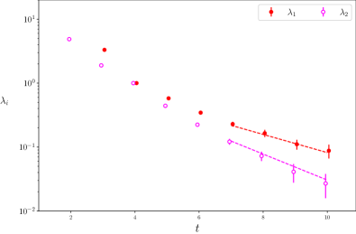
(a) Ensemble with heavier pion mass.

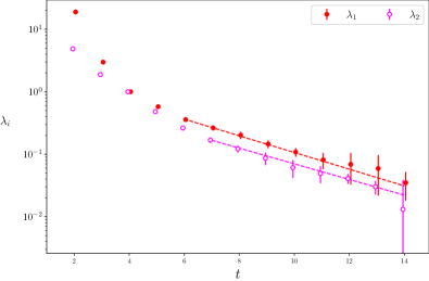
(b) Ensemble with lighter pion mass.

Figure 3: Lowest two eigenvalues for the two ensembles of this work. The dashed line indicates the fit range.

The dependence of the eigenvalues with Euclidean time is expected to be a sum of exponentials. Solving the GEVP allows one to isolate the low-lying energy states. In the limit of sufficiently large Euclidean time, each eigenvalue decays as a single exponential:

$$\lambda_{i}(t)\longrightarrow A_{i}e^{-E_{i}t},$$ (24)

which holds up to effects that are exponentially suppressed with the time extent of the lattice—thermal effects. The corresponding exponents, $E_{i}$, are associated to one energy level of the studied channel.

The dependence of the eigenvalues with Euclidean time is shown in Fig. 3. The dashed lines depict the best fit in the chosen fit interval. Note that we do not include in the fits the region in which the $\widetilde{C}_{\sigma\sigma}$ correlator is dominated by noise.

A summary of the extracted energy levels—in units of the pion mass—is given in Tab. 3 and in Fig. 4. As can be seen, the central value of the lowest energy is well below threshold, and the second level is around the two-particle threshold in both cases. The physical interpretation of these states can only be discussed after inspecting the scattering amplitude. In particular, to answer whether the lowest state corresponds to a bound state, or an attractive scattering state. This will be addressed in the next subsection.

Ensemble	$E_{1}/M_{\pi}$	$\chi^{2}_{\rm red}$	$[t_{i},t_{f}]$	$E_{2}/M_{\pi}$	$\chi^{2}_{\rm red}$	$[t_{i},t_{f}]$
Heavy	1.59(34)	1.47	[7,10]	2.27(28)	0.25	[7,10]
Light	1.81(22)	0.18	[7,14]	1.93(18)	0.30	[6,14]

Table 3: Two-particle energy levels in the singlet channel extracted from the fits in Fig. 3. We show the $\chi^{2}$ per degree of freedom, $\chi^{2}_{\rm red}=\chi^{2}/\text{dof}$, and the fit range for each level.

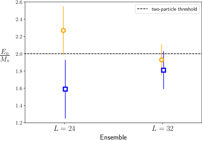
Figure 4: Energy levels obtained from our simulations. The blue square represents the lowest state, and the orange circle the first excited state.

IV.3 Results for the scattering amplitude

We are now in the position to explore the scattering amplitude in the singlet channel using the Lüscher method. For this, we insert the energy levels of Tab. 3 into the two-particle quantization condition in Eq. 14.

The corresponding points in the phase shift are shown in Fig. 5 for both ensembles, where we also include the $1\sigma$ region for visualization. As can be seen in this figure, we find in both cases a point below threshold whose central value is close to the bound state condition. Even if the uncertainty is large, the most likely interpretation is that there is indeed a bound state in this channel for the explored pseudoscalar mass. The second point in the curve is around threshold, and thus could be used to constrain the scattering length of the channel. Unfortunately, the uncertainty is too large and the result is inconclusive.

We can also comment on the comparison of our results and the leading-order prediction from ChPT. This is depicted as solid grey line in Fig. 5. The LO ChPT prediction shows no sign of a bound state in the region where we seem to find one. It does however predict one bound state well below threshold, which is an artefact caused by the Adler zero Gómez Nicola et al. (2008). Moreover, the leading chiral prediction is also not able to accommodate the observed points around threshold. Thus, it seems that the value of the pseudoscalar masses of our simulations are outside of the window for which leading-order ChPT is a good description.

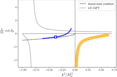
(a)   Ensemble with heavier pion mass.

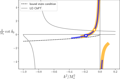
(b)   Ensemble with lighter pion mass.

Figure 5: $s$-wave phase shift in the form $(k/M_{\pi})\cot\delta_{0}$ for the two ensembles of this work. The empty marker is the central value, as the shaded area represents the $1\sigma$ resulting from the quantization condition. The blue squares correspond to the lowest state, and the orange circles to the first excited state (same convention as in Fig. 4) . Note that the width of the shaded area is arbitrary, and has been chosen for illustrative purposes. We also include the leading-order chiral prediction, as well as the bound-state condition.

V Conclusion and Outlook

This work represents the first study of the singlet channel in four-dimensional gauge theories beyond QCD. Specifically, we have considered an $SU(2)$ gauge theory with two fundamental fermions that serves as a minimal template for a Composite Higgs model.

In this theory, the symmetry breaking pattern differs from that of QCD—the $SU(4)$ flavour symmetry breaks down to $Sp(4)$. Therefore, we have derived the group-theoretical setup required to analyse this scattering channel. It can also be noted that our analysis holds for generic $Sp(2N)$ gauge theories with two fundamental fermions, as the same symmetry breaking pattern is realised.

We have used two ensembles with different pion masses. Using two different operators to solve the GEVP, we have computed the lowest two energy levels. These are fed into the Lüscher quantization condition, and we have been able to put non-perturbative constraints on the singlet scattering amplitude. Interestingly, we find that leading-order chiral perturbation theory does not seem to describe the amplitude correctly, and fails in predicting a bound state around the region where we observe it.

Our results strongly suggest that in the explored region of fermion masses the sigma is most likely a stable particle, that is, a two-pion bound state. In our two ensembles, we find that $M_{\sigma}/M_{\pi}\sim 1.5-1.8$. We however expect this feature to depend strongly upon the pion mass. Therefore, more work is required to investigate discretisation effects and to reach the phenomenologically appealing region, that is, where the sigma becomes unstable. We expect to pursue this direction in a subsequent work.

Appendix A Lie algebra of $\boldsymbol{SU(4)}$

Following the convention used in Ref. Ryttov and Sannino (2008), we define

$$\begin{split}B_{1}&=\sigma_{4},B_{2}=i\sigma_{4},B_{3}=\sigma_{3},B_{4}=i\sigma_{3},\\ B_{5}&=\sigma_{1},B_{6}=i\sigma_{1},D_{4}=\sigma_{2},D_{5}=i\sigma_{2}\,,\end{split}$$ (25)

where $\sigma_{4}$ is the identity matrix, and $\sigma_{i=1,\dots,3}$ are the Pauli matrices. The ten generators of $Sp(4)$ are denoted $S^{a=1,\dots,10}$, together with the five broken generators $X^{i=1,\dots,5}$ they are a basis of the Lie Algebra of $SU(4)$. They are defined as follows:

$$\begin{split}S^{a}&=\frac{1}{2\sqrt{2}}\begin{pmatrix}\sigma_{a}&0\\ 0&-\sigma^{T}_{a}\end{pmatrix},\quad a=1,\dots,4\\ S^{a}&=\frac{1}{2\sqrt{2}}\begin{pmatrix}0&B_{a-4}\\ B_{a-4}^{\dagger}&0\end{pmatrix},\quad a=5,\dots,10\\ X^{i}&=\frac{1}{2\sqrt{2}}\begin{pmatrix}\sigma_{i}&0\\ 0&\sigma^{T}_{i}\end{pmatrix},\quad i=1,\dots,3\\ X^{i}&=\frac{1}{2\sqrt{2}}\begin{pmatrix}0&D_{i}\\ D_{i}^{\dagger}&0\end{pmatrix},\quad i=4,5~{}.\end{split}$$ (26)

The generators $S^{a}$ satisfy the relation $(S^{a})^{T}E+ES^{a}=0$. The generators are normalised so that:

$$\begin{split}{\mathrm{tr}\left[S^{a}S^{b}\right]}=\frac{1}{2}\delta^{ab},\quad&{\mathrm{tr}\left[X^{i}X^{j}\right]}=\frac{1}{2}\delta^{ij},\\ {\mathrm{tr}\left[S^{a}X^{i}\right]}&=0\,.\end{split}$$ (27)

The structure constants of the algebra of $Sp(4)$ are defined as $f_{abc}=2{\mathrm{tr}\left[S^{a}[S^{b},S^{c}]\right]}$.

Appendix B Transformation under the flavour symmetry group $\boldsymbol{Sp(4)}$

Using the following relations:

$$\begin{split}\{C,\gamma_{5}\}=0,\quad C^{T}=-C,\\ \quad C^{2}=1,\quad(-i\sigma_{2})^{2}=-1,\end{split}$$ (28)

and the definitions of the Goldstone bosons interpolating fields in Eq. III.1 we find that:

$$\Pi =\frac{1}{2}\left[Q^{T}(-i\sigma_{2})C\gamma_{5}X^{i}EQ+\textrm{h.c}\right]^{i=1,\dots,5}$$

$$=\frac{1}{2\sqrt{2}}\begin{pmatrix}{\pi^{-}-\pi^{+}}\\ i({\pi^{-}+\pi^{+}})\\ \sqrt{2}{\pi^{0}}\\ i\left(\Pi_{\bar{u}\bar{d}}+\Pi_{ud}\right)\\ {\Pi_{\bar{u}\bar{d}}-\Pi_{ud}}\end{pmatrix}.$$ (29)

Performing an infinitesimal transformation $Q\longrightarrow Q+i\alpha^{a}S^{a}$ where $\alpha^{a}$ are real infinitesimal parameters, we find that

$$\begin{split}\Pi&\longrightarrow\Pi+M\Pi,\quad\text{with}\\ M&=\sqrt{2}\begin{pmatrix}0&-\alpha^{3}&-\alpha^{2}&-\alpha^{7}&\alpha^{8}\\ \alpha^{3}&0&-\alpha^{1}&-\alpha^{6}&-\alpha^{5}\\ \alpha^{2}&\alpha^{1}&0&\alpha^{9}&-\alpha^{10}\\ \alpha^{7}&\alpha^{6}&-\alpha^{9}&0&\alpha^{4}\\ -\alpha^{8}&\alpha^{5}&\alpha^{10}&-\alpha^{4}&0\end{pmatrix}.\end{split}$$ (30)

Here, $M$ is an antisymmetric matrix that can be decomposed onto the algebra of $SO(5)$, therefore showing that $\Pi$ belongs to a 5-dimensional irreducible representation of $Sp(4)$. The transformation of ${\mathrm{tr}\left[\Pi\otimes\Pi\right]}$ therefore reads:

$$\begin{split}{\mathrm{tr}\left[\Pi\otimes\Pi\right]}&\longrightarrow{\mathrm{tr}\left[\Pi\otimes\Pi\right]}+{\mathrm{tr}\left[M\Pi\otimes\Pi+\Pi\otimes M\Pi\right]}\\ &={\mathrm{tr}\left[\Pi\otimes\Pi\right]}+\Pi^{T}M\Pi={\mathrm{tr}\left[\Pi\otimes\Pi\right]},\end{split}$$ (31)

where we have used that $M$ is antisymmetric in the last equality.

References

- Terazawa et al. (1977) H. Terazawa, K. Akama, and Y. Chikashige, Phys. Rev. D 15, 480 (1977).
- Terazawa (1980) H. Terazawa, Phys. Rev. D 22, 184 (1980).
- Kaplan and Georgi (1984) D. B. Kaplan and H. Georgi, Phys. Lett. B 136, 183 (1984).
- Kaplan et al. (1984) D. B. Kaplan, H. Georgi, and S. Dimopoulos, Phys. Lett. B 136, 187 (1984).
- Dugan et al. (1985) M. J. Dugan, H. Georgi, and D. B. Kaplan, Nucl. Phys. B 254, 299 (1985).
- Bardeen et al. (1986) W. A. Bardeen, C. N. Leung, and S. T. Love, Phys. Rev. Lett. 56, 1230 (1986).
- Leung et al. (1986) C. N. Leung, S. T. Love, and W. A. Bardeen, Nucl. Phys. B 273, 649 (1986).
- Yamawaki et al. (1986) K. Yamawaki, M. Bando, and K.-i. Matumoto, Phys. Rev. Lett. 56, 1335 (1986).
- Weinberg (1976) S. Weinberg, Phys. Rev. D 13, 974 (1976), [Addendum: Phys.Rev.D 19, 1277–1280 (1979)].
- Susskind (1979) L. Susskind, Phys. Rev. D 20, 2619 (1979).
- Hochberg et al. (2014) Y. Hochberg, E. Kuflik, T. Volansky, and J. G. Wacker, Phys. Rev. Lett. 113, 171301 (2014), eprint 1402.5143.
- Tsai et al. (2020) Y.-D. Tsai, R. McGehee, and H. Murayama (2020), eprint 2008.08608.
- Contino et al. (2011) R. Contino, D. Marzocca, D. Pappadopulo, and R. Rattazzi, JHEP 10, 081 (2011), eprint 1109.1570.
- Bharucha et al. (2021) A. Bharucha, G. Cacciapaglia, A. Deandrea, N. Gaur, D. Harada, F. Mahmoudi, and K. Sridhar, JHEP 09, 069 (2021), eprint 2012.09470.
- Bellazzini et al. (2016) B. Bellazzini, R. Franceschini, F. Sala, and J. Serra, JHEP 04, 072 (2016), eprint 1512.05330.
- Bizot et al. (2017) N. Bizot, M. Frigerio, M. Knecht, and J.-L. Kneur, Phys. Rev. D 95, 075006 (2017), eprint 1610.09293.
- Niehoff et al. (2017) C. Niehoff, P. Stangl, and D. M. Straub, JHEP 04, 117 (2017), eprint 1611.09356.
- Buarque Franzosi et al. (2020) D. Buarque Franzosi, G. Cacciapaglia, and A. Deandrea, Eur. Phys. J. C 80, 28 (2020), eprint 1809.09146.
- Aoki et al. (2013) Y. Aoki, T. Aoyama, M. Kurachi, T. Maskawa, K.-i. Nagai, H. Ohki, E. Rinaldi, A. Shibata, K. Yamawaki, and T. Yamazaki (LatKMI), Phys. Rev. Lett. 111, 162001 (2013), eprint 1305.6006.
- Aoki et al. (2014) Y. Aoki et al. (LatKMI), Phys. Rev. D 89, 111502 (2014), eprint 1403.5000.
- Fodor et al. (2015) Z. Fodor, K. Holland, J. Kuti, S. Mondal, D. Nogradi, and C. H. Wong, PoS LATTICE2014, 244 (2015), eprint 1502.00028.
- Brower et al. (2016) R. C. Brower, A. Hasenfratz, C. Rebbi, E. Weinberg, and O. Witzel, Phys. Rev. D 93, 075028 (2016), eprint 1512.02576.
- Arthur et al. (2016a) R. Arthur, V. Drach, A. Hietanen, C. Pica, and F. Sannino (2016a), eprint 1607.06654.
- Hasenfratz et al. (2017) A. Hasenfratz, C. Rebbi, and O. Witzel, Phys. Lett. B 773, 86 (2017), eprint 1609.01401.
- Appelquist et al. (2016) T. Appelquist et al., Phys. Rev. D 93, 114514 (2016), eprint 1601.04027.
- Athenodorou et al. (2017) A. Athenodorou, E. Bennett, G. Bergner, D. Elander, C. J. D. Lin, B. Lucini, and M. Piai, PoS LATTICE2016, 232 (2017), eprint 1702.06452.
- Appelquist et al. (2019) T. Appelquist et al. (Lattice Strong Dynamics), Phys. Rev. D 99, 014509 (2019), eprint 1807.08411.
- Lee et al. (2018) J.-W. Lee, E. Bennett, D. K. Hong, C. J. D. Lin, B. Lucini, M. Piai, and D. Vadacchino, PoS LATTICE2018, 192 (2018), eprint 1811.00276.
- Bennett et al. (2019) E. Bennett, D. K. Hong, J.-W. Lee, C. J. D. Lin, B. Lucini, M. Piai, and D. Vadacchino, JHEP 12, 053 (2019), eprint 1909.12662.
- Appelquist et al. (2021) T. Appelquist et al. (LSD) (2021), eprint 2106.13534.
- Drach et al. (2021) V. Drach, T. Janowski, C. Pica, and S. Prelovsek, JHEP 04, 117 (2021), eprint 2012.09761.
- Cacciapaglia and Sannino (2014) G. Cacciapaglia and F. Sannino, JHEP 04, 111 (2014), eprint 1402.0233.
- Cacciapaglia et al. (2020) G. Cacciapaglia, C. Pica, and F. Sannino, Phys. Rept. 877, 1 (2020), eprint 2002.04914.
- Bijnens and Lu (2011) J. Bijnens and J. Lu, JHEP 03, 028 (2011), eprint 1102.0172.
- Del Debbio et al. (2010) L. Del Debbio, A. Patella, and C. Pica, Phys. Rev. D 81, 094503 (2010), eprint 0805.2058.
- Wilson (1974) K. G. Wilson, Phys. Rev. D 10, 2445 (1974).
- Sheikholeslami and Wohlert (1985) B. Sheikholeslami and R. Wohlert, Nucl. Phys. B 259, 572 (1985).
- Lüscher and Weisz (1985) M. Lüscher and P. Weisz, Commun. Math. Phys. 97, 59 (1985), [Erratum: Commun.Math.Phys. 98, 433 (1985)].
- Arthur et al. (2016b) R. Arthur, V. Drach, M. Hansen, A. Hietanen, C. Pica, and F. Sannino, Phys. Rev. D 94, 094507 (2016b), eprint 1602.06559.
- Martinelli et al. (1995) G. Martinelli, C. Pittori, C. T. Sachrajda, M. Testa, and A. Vladikas, Nucl. Phys. B 445, 81 (1995), eprint hep-lat/9411010.
- Ryttov and Sannino (2008) T. A. Ryttov and F. Sannino, Phys. Rev. D 78, 115010 (2008), eprint 0809.0713.
- Lüscher and Wolff (1990) M. Lüscher and U. Wolff, Nucl. Phys. B 339, 222 (1990).
- Lüscher (1986a) M. Lüscher, Commun. Math. Phys. 105, 153 (1986a).
- Lüscher (1991a) M. Lüscher, Nucl. Phys. B 354, 531 (1991a).
- Lüscher (1991b) M. Lüscher, Nucl. Phys. B 364, 237 (1991b).
- Rummukainen and Gottlieb (1995) K. Rummukainen and S. A. Gottlieb, Nucl. Phys. B 450, 397 (1995), eprint hep-lat/9503028.
- Kim et al. (2005) C. h. Kim, C. T. Sachrajda, and S. R. Sharpe, Nucl. Phys. B 727, 218 (2005), eprint hep-lat/0507006.
- He et al. (2005) S. He, X. Feng, and C. Liu, JHEP 07, 011 (2005), eprint hep-lat/0504019.
- Bernard et al. (2011) V. Bernard, M. Lage, U. G. Meißner, and A. Rusetsky, JHEP 01, 019 (2011), eprint 1010.6018.
- Briceño and Davoudi (2013) R. A. Briceño and Z. Davoudi, Phys. Rev. D 88, 094507 (2013), eprint 1204.1110.
- Briceño (2014) R. A. Briceño, Phys. Rev. D 89, 074507 (2014), eprint 1401.3312.
- Romero-López et al. (2018) F. Romero-López, A. Rusetsky, and C. Urbach, Phys. Rev. D 98, 014503 (2018), eprint 1802.03458.
- Luu and Savage (2011) T. Luu and M. J. Savage, Phys. Rev. D 83, 114508 (2011), eprint 1101.3347.
- Göckeler et al. (2012) M. Göckeler, R. Horsley, M. Lage, U. G. Meißner, P. E. L. Rakow, A. Rusetsky, G. Schierholz, and J. M. Zanotti, Phys. Rev. D 86, 094513 (2012), eprint 1206.4141.
- Briceño et al. (2018a) R. A. Briceño, J. J. Dudek, and R. D. Young, Rev. Mod. Phys. 90, 025001 (2018a), eprint 1706.06223.
- Guo et al. (2018) D. Guo, A. Alexandru, R. Molina, M. Mai, and M. Döring, Phys. Rev. D 98, 014507 (2018), eprint 1803.02897.
- Fu and Chen (2018) Z. Fu and X. Chen, Phys. Rev. D 98, 014514 (2018), eprint 1712.02219.
- Mai et al. (2019) M. Mai, C. Culver, A. Alexandru, M. Döring, and F. X. Lee, Phys. Rev. D 100, 114514 (2019), eprint 1908.01847.
- Briceno et al. (2017) R. A. Briceno, J. J. Dudek, R. G. Edwards, and D. J. Wilson, Phys. Rev. Lett. 118, 022002 (2017), eprint 1607.05900.
- Briceño et al. (2018b) R. A. Briceño, J. J. Dudek, R. G. Edwards, and D. J. Wilson, Phys. Rev. D 97, 054513 (2018b), eprint 1708.06667.
- Liu et al. (2017) L. Liu et al., Phys. Rev. D 96, 054516 (2017), eprint 1612.02061.
- Iritani et al. (2017) T. Iritani, S. Aoki, T. Doi, T. Hatsuda, Y. Ikeda, T. Inoue, N. Ishii, H. Nemura, and K. Sasaki, Phys. Rev. D 96, 034521 (2017), eprint 1703.07210.
- Lüscher (1986b) M. Lüscher, Commun. Math. Phys. 104, 177 (1986b).
- König and Lee (2018) S. König and D. Lee, Phys. Lett. B 779, 9 (2018), eprint 1701.00279.
- Bijnens and Lu (2009) J. Bijnens and J. Lu, JHEP 11, 116 (2009), eprint 0910.5424.
- Blanton et al. (2020) T. D. Blanton, F. Romero-López, and S. R. Sharpe, Phys. Rev. Lett. 124, 032001 (2020), eprint 1909.02973.
- Gómez Nicola et al. (2008) A. Gómez Nicola, J. R. Peláez, and G. Ríos, Phys. Rev. D 77, 056006 (2008), eprint 0712.2763.