The BH-PSR Gravitational Molecule

Abstract

While axion-clouded black hole (BH) encounters another massive star, a “gravitational molecule” (a novel binary system) can form. The axion cloud then evolves at the binary hybrid orbitals, as it occurs at microscopic level to electron cloud in a chemical molecule. To show this picture, we develop a semi-analytical formalism using the method of linear combination of atomic orbitals with the Born-Oppenheimer approximation, and apply it to a BH-PSR (pulsar) gravitational molecule. An oscillating axion-cloud profile and a perturbed binary rotation, together with unique and novel detection signals, are then predicted. Remarkably, the proposed PSR timing and polarization observables, namely the oscillation of periastron time shift and the birefringence with multiple modulations, correlate in pattern, and thus can be properly combined to strengthen the detection.

Introduction — “Superradiance” of bosons can occur near a spinning black hole (BH) Damour et al. (1976); Bekenstein (1973); Bekenstein and Schiffer (1998); Brito et al. (2015); Brill et al. (1972); Rosa (2010); Detweiler (1980); Dolan (2007); Endlich and Penco (2017); Yoshino and Kodama (2014); Arvanitaki and Dubovsky (2011), if their Compton wavelength is comparable to the BH horizon. Then certain energy levels of this BH get populated with these ultralight bosons, by extracting its own angular momentum and energy. Eventually a “gravitational atom” with a BH “nucleus” forms. Here $|211\rangle$ Detweiler (1980), a state with gravitational principal, orbital and magnetic quantum numbers $\{n=2,l=1,m=1$}, may serve as a leading mode.

Among the candidates of ultralight bosons, axion is especially interesting. Axion is originally proposed to solve strong CP problem Peccei and Quinn (1977a, b); Weinberg (1978); Wilczek (1978); Dine and Fischler (1983); Preskill et al. (1983); Abbott and Sikivie (1983). This concept is later generalized to string theory Svrcek and Witten (2006); Arvanitaki et al. (2010); Cicoli et al. (2012). The axion and axion-like particles (we will not distinguish them below) can serve as a primary component of dark matter in the universe, with a mass ranging from sub eV to $\sim 10^{-22}$ eV Marsh (2016).

The advent of multi-messenger astronomy provides a great opportunity to investigate gravitational atoms and explore the physics of ultralight bosons, which has motivated extensive studies in literatures (see, e.g., Irastorza and Redondo (2018); Brito et al. (2017); Chen et al. (2020); Davoudiasl and Denton (2019); Plascencia and Urbano (2018); Isi et al. (2019); East (2018); Marsh and Hoof (2021); Yuan et al. (2021); Baryakhtar et al. (2021); Ng et al. (2021, 2020); Kavic et al. (2020); Wen et al. (2021); Chia (2020); Siemonsen and East (2020); Ghosh et al. (2019)). Recently, the study was extended to gravitational-atom (GA) binaries, with their companion being either a BH Zhang and Yang (2020); Fernandez et al. (2019); Baumann et al. (2019a) or a pulsar (PSR) Ding et al. (2021); Kavic et al. (2020). Especially, the Landau-Zener enegy-level transitions induced by the companion’s gravitational perturbation have been suggested to probe for gravitational atoms (or “gravitational collider” physics) Baumann et al. (2019a, b); Baumann et al. (2020); Ding et al. (2021); Tong et al. (2021).

However, while a GA encounters a BH or a PSR or has such a massive companion, a more generic picture could be the formation of gravitational molecule (GM). Due to orbital hybridization, the axion cloud of GA will flow or partly flow to its companion. This mechanism is different from mass transfer of Type Ia supernova binaries: (1) the axion cloud is generated as a coherent field while the transferred matter in the latter case is particle-like; and (2) the flow can cross the boundary of Roche lobe, where no Newtonian matter transfer takes place. Such a system thus can be viewed as a macroscopic counterpart of a diatomic molecule.

Although the condensate of the ultralight bosons near a binary has been known Ikeda et al. (2021), analyzing the dynamical evolution of such a GM and its observational phenomenology is highly involved. In this letter we will develop a semi-analytical formalism, inspired by quantum chemistry, to address this problem. We will construct a simplified model for the given GM, analyze its orbital hybridization and state evolution using the method of linear combination of atomic orbitals (LCAO) che with a Born-Oppenheimer approximation, and then explore its detection signals in astronomy. Such a methodology allows us to study the generic features of GMs without involving much numerical work. We would view it to be a starting point for the more refined analyses later.

For concreteness, we will work on a BH-PSR GM (though the developed analysis formalism can be applied to a BH-BH GM also). The specification of a PSR as the companion is because the BH-PSR binaries are expected to be future precision astronomical laboratories. According to recent estimations Chattopadhyay et al. (2021); Shao and Li (2018, 2021), in our galaxy $\sim\mathcal{O}(10$ $-10^{3})$ stelar BH-PSR binaries are yet to be discovered. The study of such a GM may benefit from not only its gravitational-wave (GW) signals, but also the PSR timing and polarization signals. Recall, in history the timing signals of PSR B1913+16 have provided the first evidence on GWs Taylor and Weisberg (1982, 1989); Weisberg et al. (2010). So, a BH-PSR GM will be highly valuable for multi-messenger astronomy.

Modeling the BH-PSR GM — We model the BH-PSR GM as follows. At $t\leq 0_{-}$, the axion-clouded BH stays in an initial state of $|211\rangle$, with the PSR’s gravitational perturbation being negligibly small. Here the gravitational “Bohr radius” and “fine-structure constant” of this BH are given by Baumann et al. (2019b)

$$r_{c} = \frac{1}{m_{\phi}\alpha}=1.3\times 10^{4}\times\left(\dfrac{0.015}{\alpha}\right)\left(\dfrac{10^{-12}\text{eV}}{m_{\phi}}\right)\text{km}\ ,$$

$$\alpha = GM_{\rm BH}m_{\phi}=0.015\left(\dfrac{M_{\rm BH}}{2M_{\odot}}\right)\left(\dfrac{m_{\phi}}{10^{-12}\text{eV}}\right)\ .$$ (1)

A percent-level $\alpha$ is then obtained for $m_{\phi}\sim 10^{-12}$ eV and $M_{\rm BH}\sim M_{\odot}$. In this case, the depletion of the axion cloud by emitting the GWs occurs at a cosmic time scale. The caused mass loss thus can be neglected. We also assume the BH’s angular velocity at its outer horizon to be

$$\Omega_{\rm BH}<\frac{E_{211}}{m}\sim m_{\phi}\ .$$ (2)

Here $E_{211}$ is the $|211\rangle$ eigenenergy. This implies that no more axions will be produced by superradiance. At $t=0_{+}$, the axion cloud starts to evolve at the hybrid orbitals of this molecule, where the BH and its companion is separated with $R=R_{0}$.

This picture models the diabatic formation of gravitational binaries by, e.g., three-body exchange Valtonen and Karttunen (2006); Hills (1976); Clark (1975); Stoeckley (1981); Heggie (2003); Hills and Fullerton (1980); Ziosi et al. (2014); Celoria et al. (2018) (one of the main mechanisms for binary production by which most stellar BH-BH binaries in star clusters may have produced Hills and Fullerton (1980); Ziosi et al. (2014); Celoria et al. (2018)). Its application can be also extended to the GMs with a prompt orbit shrinking (from $R=R_{0}^{\prime}$ to $R=R_{0}$ with $R_{0}^{\prime}>R_{0}$, at $t=0_{+}$) caused by either three-body hardening Valtonen and Karttunen (2006); Colpi et al. (2009); Celoria et al. (2018) or resonant level transition Baumann et al. (2020), where the axion-could initial state is defined at $R=R_{0}^{\prime}$. The binary rotation, which we assume to be circular (with its angular velocity $\omega=|\boldsymbol{\omega}|=\omega_{i}$ and period $T_{b}=T_{b,i}$ initially) and anti-parallel to the BH spin here, will be perturbed by the axion-cloud evolution then. Notably, a fully-occupied $|211\rangle$ state has total energy $M_{\rm AC}\sim Nm_{\phi}$ with the occupation number $N\sim[10f_{\phi}/(\alpha^{3/2}m_{\phi})]^{2}$ being set by Bosenova limit Yoshino and Kodama (2012). $f_{\phi}$ is axion decay constant. Assuming $M_{\rm BH}=M_{\rm PSR}=M$ (the BH and the PSR then share the $\alpha$ and $r_{c}$ values), we have

$$\varepsilon=\frac{M_{\rm AC}}{M}\lesssim\frac{m_{e}}{m_{p}}\ll 1$$ (3)

for $M\sim M_{\odot}$ and $f_{\phi}\lesssim 10^{13}$ GeV at $m_{\phi}=10^{-12}$eV Arvanitaki et al. (2015). Here $m_{e}/m_{p}$ is the mass ratio of electron and proton. This implies that, given the same amount of kinetic energy, the relative change to the BH-PSR motion is much smaller than that of the axion cloud. This analysis thus can be pursued in the spirit of the Born-Oppenheimer approximation in quantum chemistry. Explicitly, we separate our analysis to two steps. We first analyze the axion-cloud evolution using the LCAO method, assuming the BH-PSR rotation to be unperturbed. Then we solve the perturbations to the BH-PSR rotation with angular-momentum and energy conservation .

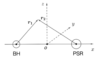
Figure 1: Coordinate system for the rotating reference frame of the BH-PSR GM.

The coordinate system for the rotating reference frame of this BH-PSR GM is demonstrated in Fig. 1, where the original point is positioned at the BH-PSR barycenter, and $x$- and $z$-axes are defined by the BH-PSR line and the BH spinning direction, respectively. The axion-cloud profile, as a real scalar field, is described by

$$\phi(t,{\bf r})=\dfrac{1}{\sqrt{2m_{\phi}}}\left[\psi(t,{\bf r})\exp{(-im_{\phi}t)}+{\rm h.c.}\right]\ .$$ (4)

Here $\psi$ is complex and satisfies gravitational Schrodinger equation (up to higher-order curvature corrections)

$$i\dfrac{\partial}{\partial t}\psi(t,{\bf r})=\left(\dfrac{{\bf p}^{2}}{2m_{\phi}}+V_{1}+V_{2}+V_{c}\right)\psi(t,{\bf r})\ ,$$ (5)

where $V_{1,2}=-\alpha/|{\bf r_{1,2}}|$ are the BH and the PSR gravitation potentials, and $V_{c}=-{\boldsymbol{\omega}}\cdot{\bf L}=-{\boldsymbol{\omega}}\cdot({\bf r}\times{\bf p})$ is the inertia potential of axion cloud arising from the binary rotation Anandan and Suzuki (2003). All of them are of order $\sim\mathcal{O}(\alpha^{2})$ in the length unit of $r_{c}$ (note $\omega=\left(2GM/R^{3}\right)^{1/2}=\sqrt{2}\alpha^{2}m_{\phi}/\left(R/r_{c}\right)^{3/2}$). The Coriolis and centrifugal forces will appear in the Heisenberg equation of ${\bf r}$ then. At last, for $R<5r_{c}$ the radius of Roche lobe (at Lagrange-point-2 side) Johnston (2018) becomes $<2r_{c}$, at which the initial axion-cloud distribution is expected to be peaked. Part of the axion cloud might be pushed far away from the binary then. So, our study will focus on the scenario with $R>5r_{c}$.

Orbital Hybridization and State Evolution — We introduce a basis for $n_{i}=2$ atomic states ($i=1$, 2 denote “BH” and “PSR” respectively): $|s_{i}\rangle=|200_{,i}\rangle$ and $|p_{x,i}\rangle=(|211_{,i}\rangle-|21-1_{,i}\rangle)/\sqrt{2}$, $|p_{y,i}\rangle=(|211_{,i}\rangle+|21-1_{,i}\rangle)/\sqrt{2}i$. Here $|s_{i}\rangle$ is spherically symmetric in space, while $|p_{x(y),i}\rangle$ is aligned with $x(y)$-axis. Note, $|p_{z,i}\rangle$ is irrelevant here since it does not couple with the others via the Hamiltonian. Then we can define a hybrid basis, including the $s_{1}-s_{2}$ bond ($\sigma_{s}$) and anti-bond ($\sigma_{s}^{*}$), the $p_{x}-p_{x}$ bond ($\sigma$) and anti-bond ($\sigma^{*}$), and the $p_{y}-p_{y}$ bond ($\pi$) and anti-bond ($\pi^{*}$). Explicitly we have

$$|\sigma_{s}\rangle=A_{\sigma_{s}}\left(|s_{1}\rangle+|s_{2}\rangle\right),\ \ \ |\sigma_{s}^{*}\rangle=A_{\sigma_{s}^{*}}\left(|s_{1}\rangle-|s_{2}\rangle\right),$$ (6)

$$|\sigma\rangle=A_{\sigma}\left(|p_{x,1}\rangle+|p_{x,2}\rangle\right),\ |\sigma^{*}\rangle=A_{\sigma^{*}}\left(|p_{x,1}\rangle-|p_{x,2}\rangle\right),$$

$$|\pi\rangle=A_{\pi}\left(|p_{y,1}\rangle+|p_{y,2}\rangle\right),\ |\pi^{*}\rangle=A_{\pi^{*}}\left(|p_{y,1}\rangle-|p_{y,2}\rangle\right),$$

with the normalization coefficients

$$A_{\sigma_{s},\sigma,\pi}=\frac{1}{\sqrt{2\left(1+S_{s,x,y}\right)}},\ A_{\sigma_{s}^{*},\sigma^{*},\pi^{*}}=\frac{1}{\sqrt{2\left(1-S_{s,x,y}\right)}}\ .$$ (7)

Here $S_{s}=\langle s_{1}|s_{2}\rangle$, $S_{x}=\langle p_{x,1}|p_{x,2}\rangle$ and $S_{y}=\langle p_{y,1}|p_{y,2}\rangle$ are overlap integrals of $s$, $p_{x}$ and $p_{y}$, respectively. The axion-cloud initial profile is then described by

$$|211_{,1}\rangle = \frac{\sqrt{2}}{2}(|p_{x,1}\rangle+i|p_{y,1}\rangle)$$

$$= \frac{1}{2\sqrt{2}}\left(\frac{|\sigma\rangle}{A_{\sigma}}+\frac{|\sigma^{*}\rangle}{A_{\sigma}^{*}}+i\frac{|\pi\rangle}{A_{\pi}}+i\frac{|\pi^{*}\rangle}{A_{\pi}^{*}}\right)\ .$$

Note, both bases are approximately orthogonal only. For the convenience, below we will analyze the orbital hybridization in the hybrid basis and study the observational phenomenology in the atomic basis.

In quantum chemistry, the 2$s$-$2p$ orbital hybridization is often ignored for homonuclear diatomic molecules such as $O_{2}$ and $F_{2}$, where the 2$s$-$2p$ energy-level splitting is relatively big. But, this does not apply here, since $|\langle\sigma_{s}(\sigma)|V_{1}+V_{2}|\sigma(\sigma_{s})\rangle|>|\langle\sigma_{s}|V_{1}+V_{2}|\sigma_{s}\rangle-\langle\sigma|V_{1}+V_{2}|\sigma\rangle|$. This is reminiscent of some other period-2 diatomic molecules such as $N_{2}$ and $C_{2}$, where Coulomb repulsion from the $\sigma$ electrons reduces the 2$s$-$2p$ energy-level splitting and hence enhances its orbital hybridization. Differently, however, the axion-cloud inertia potential correlates the $\sigma(\sigma^{*})$ and $\pi^{*}(\pi)$ states also, because of $\langle\pi^{*}(\pi)|V_{c}|\sigma(\sigma^{*})\rangle\neq 0$. This effect breaks $\sigma$ symmetry (a cylindrical symmetry about $x$-axis) and finally yields a mixing for $\{\sigma_{s},\sigma,\pi^{*}\}$ and $\{\sigma_{s}^{*},\sigma^{*},\pi\}$. We denote their respective energy eigenstates as $\xi_{1,2,3}$ and $\xi_{1,2,3}^{*}$.

The Hamiltonian matrix for the BH-PSR GM is block-diagonal in the hybrid basis, given by $(H_{\phi})_{\rm diag}=\alpha^{2}m_{\phi}\times\{A_{\phi},B_{\phi}\}+m_{\phi}\times I$. Here

$$\left.\begin{array}[]{lr}A_{\phi}\\ B_{\phi}\end{array}\right\} = \begin{pmatrix}-\dfrac{1}{8}-\epsilon&3\epsilon^{2}&0\\ 3\epsilon^{2}&-\dfrac{1}{8}-\epsilon-12\epsilon^{3}&i\sqrt{2}\epsilon^{3/2}\\ 0&-i\sqrt{2}\epsilon^{3/2}&-\dfrac{1}{8}-\epsilon+6\epsilon^{3}\end{pmatrix}$$ (12)

$$+\mathcal{O}(\epsilon^{-3}\exp(-1/2\epsilon))$$

are identical up to an exponentially-suppressed factor. $\epsilon=\frac{r_{c}}{R}$ is a perturbation measure for the matrix entries. The eigenvalues are then solved to be

$$\frac{E_{\xi}-m_{\phi}}{\alpha^{2}m_{\phi}}=A\left(1,1,1\right)+\left(-\sqrt{2}\epsilon^{3\over 2},0,\sqrt{2}\epsilon^{3\over 2}\right)+o(\epsilon^{\frac{5}{2}})$$ (13)

with $A=-\frac{1}{8}-\epsilon$. The $\xi_{a}$ and $\xi_{a}^{*}$ profiles and their energy eigenvalues are both $R$-dependent. In the limit of $R\gg r_{c}$ or $\epsilon\ll 1$, the splitting between $E_{\xi_{i}^{(*)}}$ and $E_{\xi_{j}^{(*)}}$ ($i\neq j$) is mainly determined by $\sqrt{2}\epsilon^{3/2}$, while the one between $E_{\xi_{i}}$ and $E_{\xi_{i}^{*}}$ is exponentially suppressed. These features are demonstrated in Fig. 2. The set of $E_{\xi_{i}^{(*)}}$ define several time scales to characterize this system, including

$$T_{i}^{\pm}=\frac{4\pi}{|E_{\xi_{i}}\pm E_{\xi_{i}^{*}}|},\ T_{A}^{\pm}=\frac{4\pi}{|(E_{\xi_{2}}-E_{\xi_{3}})\pm(E_{\xi_{2}^{*}}-E_{\xi_{3}^{*}})|},$$ (14)

where $T_{A}^{+}\sim T_{b,i}$ and $T_{i}^{-}$ is exponentially lengthened.

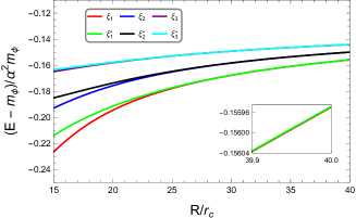
Figure 2: Energy eigenvalues of the $n=2$ BH-PSR hybrid states versus the BH-PSR separation.

As $|211_{,1}\rangle$ is not stationary, the axion cloud will evolve in space. In the benchmark scenario defined by Tab. 1, we find (see App. A for its calculation).

$$\phi(t,{\bf r}) =\dfrac{\sqrt{\varepsilon M}}{m_{\phi}}\times$$ (15)

$$[(-0.009C_{1}^{+}C_{1}^{-}-0.210C_{2}^{+}C_{2}^{-}+0.218C_{3}^{+}C_{3}^{-})s_{1}+$$

$$(-0.009S_{1}^{+}S_{1}^{-}-0.210S_{2}^{+}S_{2}^{-}+0.218S_{3}^{+}S_{3}^{-})s_{2}+$$

$$(0.038C_{1}^{+}C_{1}^{-}-0.002C_{2}^{+}C_{2}^{-}+0.963C_{3}^{+}C_{3}^{-})p_{x,1}+$$

$$(0.038S_{1}^{+}S_{1}^{-}-0.002S_{2}^{+}S_{2}^{-}+0.963S_{3}^{+}S_{3}^{-})p_{x,2}+$$

$$(-0.035S_{1}^{+}C_{1}^{-}+0.099S_{2}^{+}C_{2}^{-}+0.936S_{3}^{+}C_{3}^{-})p_{y,1}+$$

$$(-0.035C_{1}^{+}S_{1}^{-}+0.100C_{2}^{+}S_{2}^{-}+0.936C_{3}^{+}S_{3}^{-})p_{y,2}]\ ,$$

where $S_{i}^{\pm}=\sin\left(\dfrac{2\pi t}{T_{i}^{\pm}}\right)$ and $C_{i}^{\pm}=\cos\left(\dfrac{2\pi t}{T_{i}^{\pm}}\right)$. At $t=0_{+}$, $\phi(t,{\bf r})$ is reduced to $\propto p_{x,1}$. It implies that the axion cloud is distributed near the BH initially. Soon after that, the PSR gets surrounded by the axion cloud massively. As shown in Fig. 3, the axion cloud oscillates between the BH and the PSR with an approximate period of $T_{3}^{-}$.

$M(M_{\odot})$	$\alpha$	$m_{\phi}$(eV)	$f_{\phi}$(GeV)	$c_{\gamma}$	$r_{c}$(km)	$R_{0}(r_{c})$
2	$0.015$	$2\times 10^{-12}$	$5\times 10^{12}$	$3\times 10^{3}$	$1.3\times 10^{4}$	$40$
$h_{e}$(km)	$T_{b,i}$(s)	$T_{1}^{-}$(s)	$T_{2}^{-}$(s)	$T_{3}^{-}$(s)	$T_{A}^{+}$(s)	$T_{A}^{-}$(s)
500	$3.3\times 10^{3}$	$3.1\times 10^{7}$	$3.2\times 10^{7}$	$1.2\times 10^{8}$	$3.2\times 10^{3}$	$4.4\times 10^{7}$

Table 1: Benchmark scenario of the BH-PSR GM.

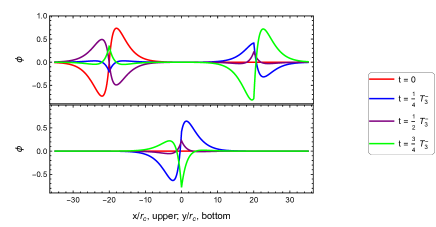
Figure 3: Axion-cloud oscillation for the BH-PSR GM, along $x$-axis (upper; $y=z=0$) and $y$-axis (bottom; $x=20r_{c}$, $z=0$).

With the message on the axion-cloud evolution, now we are able to analyze its perturbation to the BH-PSR orbital rotation, by imposing the conditions of angular-momentum and energy conservation. For this purpose, let us define $\beta=(R-R_{0})/R_{0}$ and $\gamma=(\omega-\omega_{i})/\omega_{i}$ to characterize these effects. During this evolution, the axion-cloud energy is not conserved. First, the transition of axion cloud from the BH $|211\rangle$ state at $t=0_{-}$ to the binary hybrid states at $t=0_{+}$ causes a shift to its energy. Second, the axion cloud is not in a stationary state for $t\geq 0_{+}$ and its energy hence will oscillate as it evolves at the GM hybrid orbitals. Such variations in the axion-cloud energy is interchanged to the binary by gravitational interaction, resulting in non-trivial time dependence for $\beta(t)$ and accordingly for $\gamma(t)$ due to the angular-momentum conservation. The axion cloud can interchange its angular momentum with the binary also:

$$[\hat{L}_{\text{AC}},H_{\phi}]=\frac{-i\alpha R}{2}\left(\frac{y}{r_{1}^{3}}-\frac{y}{r_{2}^{3}}\right)\equiv T_{G}\neq 0\ .$$ (16)

Here $\hat{L}_{\text{AC}}=(x\hat{p}_{y}-y\hat{p}_{x})$ is the intrinsic angular-momentum operator of axion cloud along $z$-axis , and $T_{G}$ is gravitational torque. But, this effect enters at a higher order of $\epsilon$ only. Analytically solving $\beta(t)$ and $\gamma(t)$ in the full time domain is a challenging task. For the purpose of demonstration, let us consider the limit of $t\ll T_{A}^{-}$ (note $T_{A}^{+}\ll T_{A}^{-}$) and extend this study to a full time domain later Liu et al. (in preparation). In this limit, we have (see App. B for its derivation)

$$\begin{split}\beta(t)&=-\frac{1}{2}\gamma(t)\\ &=\pm\varepsilon^{1/2}\left[1.1\times 10^{-2}+1.9\cos\left(\dfrac{2\pi t}{T_{A}^{+}}\right)\right]\ ,\end{split}$$ (17)

with $T_{A}^{+}\approx T_{b}$. Notably, the magnitudes of $\beta$ and $\gamma$ are both $\propto\varepsilon^{1/2}$ at the leading order, which well-justifies the Born-Oppenheimer approximation taken in this study.

Astronomical Detection — The axion-cloud evolution and its perturbation to the binary rotation yield unique and novel signals for detecting the BH-PSR GMs. Here let us consider two PSR observables, namely periastron time shift and birefringence, which are based on its timing and polarization signals respectively. We postpone the study on the GW probe to a later time Liu et al. (in preparation).

The periastron time shift is a measure of the time dependence of the PSR orbital period, given by Taylor (1994); Ding et al. (2021)

$$\Delta t_{P}(t)=t-T_{b}(0)\int_{0}^{t}\dfrac{1}{T_{b}(t^{\prime})}dt^{\prime}\ .$$ (18)

It is modulated by the perturbation to the binary rotation, through the $\gamma(t)$ factor in $T_{b}(t)=T_{b,i}/(1+\gamma(t))$.

The birefringence Carroll et al. (1990) occurs when the linearly polarized PSR light travels across an axion field Liu et al. (2020), due to the parity-violating interaction: $\mathcal{L}\sim-\frac{1}{2}g_{\phi\gamma}\phi F_{\mu\nu}\tilde{F}^{\mu\nu}$. Here $F_{\mu\nu}$ is electromagnetic field strength and $\tilde{F}_{\mu\nu}$ is its dual; $g_{\phi\gamma}=c_{\gamma}\alpha_{em}/(4\pi f_{a})$ is the Chern-Simons coupling, currently limited to $<\left(2\times 10^{12}\text{GeV}\right)^{-1}$ for $m_{\phi}\sim 10^{-12}$eV Tanabashi et al. (2018); $c_{\gamma}$ is model-dependent and can vary from $\sim\mathcal{O}(1)$ to orders of magnitude higher Choi and Im (2016); Kaplan and Rattazzi (2016); Long (2018); Agrawal et al. (2018). The PSR polarization position angle (PA) is then varied by Harari and Sikivie (1992):

$$\Delta\Theta=g_{\phi\gamma}\left[\phi(t_{\text{r}},{\bf r}_{\text{r}})-\phi(t_{\text{e}},{\bf r}_{\text{e}})\right]\approx-g_{\phi\gamma}\phi(t_{\text{e}},{\bf r}_{\text{e}})\ .$$ (19)

Here “e” and “r” denote the spacetime points of light emission (PSR) and reception (Earth). We assume the Earth to be in the $x$-$y$ plane for simplicity. Moreover, for $R\gg r_{c}$, the contributions of the $s_{1}$, $p_{x,1}$ and $p_{y,1}$ terms in Eq. (15) are exponentially suppressed. So we have

$$\Delta\Theta\approx \left(\dfrac{c_{\gamma}}{3\times 10^{3}}\right)\left(\dfrac{M}{2M_{\odot}}\right)\left(\dfrac{m_{\phi}}{10^{-12}\text{eV}}\right)^{2}\left(\frac{h_{e}}{500{\rm km}}\right)$$

$$\times\big{[}-2.2^{\circ}S_{1}^{+}S_{1}^{-}-54.8^{\circ}S_{2}^{+}S_{2}^{-}+57.1^{\circ}S_{3}^{+}S_{3}^{-}$$

$$+3.4^{\circ}S_{3}^{+}S_{3}^{-}\cos\eta-3.3^{\circ}C_{3}^{+}S_{3}^{-}\sin\eta\big{]}\ ,$$ (20)

with $\eta=\omega_{i}\left(t-\Delta t_{P}\right)\sim\frac{2\pi t}{T_{b}}$. Here $h_{e}\sim\mathcal{O}(10^{2})-\mathcal{O}(10^{3})$ km is the emission height of the PSR light Mitra (2017). This signal is then jointly modulated by the axion-cloud oscillation and the perturbed binary rotation. As a reference, the current precision of measuring the PSR polarization PA is $\sim\mathcal{O}(1.0^{\circ})$ Tatischeff et al. (2017); Słowikowska et al. (2009); Moran et al. (2013)

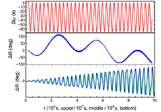
Figure 4: Signal patterns of periastron time shift (upper) and birefringence (middle, bottom) for a BH-PSR GM. The bottom panel is a zoom-in of the middle one at $0_{+}\leq t\ll T_{A}^{-}$, where the $s_{2}$ contribution is dropped and the $\Delta t_{P}$ is amplified by 10 times, for a more visual demonstration, and the reference curve (green) is drawn with $\Delta t_{P}\equiv 0$ ($i.e.$, $\eta=\omega_{i}t$).

We demonstrate the signal patterns of periastron time shift and birefringence in Fig. 4. $\Delta t_{P}(t)$ oscillates with a period $T_{A}^{+}\approx T_{b}$ and an amplitude about tens of seconds. Given the high precision of the PSR timing measurements Weisberg et al. (2010), this signal is strong. The $\Delta\Theta$ spectrum is dominated by the $s_{2}$-mode in Eq. (15), and hence mainly modulated by $T_{2}^{-}$ and $T_{3}^{-}$ through the second and third terms in Eq. (The BH-PSR Gravitational Molecule) . Moreover, a “hidden” modulation exists for this spectrum, due to the $\gamma(t)$ dependence of the $\eta$ or $T_{b}$ parameter. This modulation is manifested as an offset between the blue and green curves in the bottom panel, with a period $\sim T_{A}^{+}$ and an amplitude $\sim|\Delta t_{P}|$. Exactly it is caused by the effect measured with the periastron time shift. These two observables thus can be correlated to strengthen the detection.

Conclusion and Outlook — In this letter, we have developed a LCAO-based formalism to analyze the orbital hybridization of a BH-PSR GM and its state evolution, with the Born-Oppenheimer approximation. An oscillating axion-cloud profile and a perturbed binary rotation are then predicted, together with the unique and novel detection signals. Following this work, we can immediately see several important directions to explore.

First, draw a full picture on the GMs. Despite their rich physics, we consider mainly a BH-PSR GM with $M_{\rm BH}=M_{\rm PSR}$ so far. Generalizing this study to other possibilities, such as a variance of the analyzed one in terms of BH mass ($M_{\rm BH}\neq M_{\rm PSR}$), spin orientation, initial state, orbit eccentricity, curvature corrections, etc., is naturally expected. For example, if the BH and its companion have different mass, the orbital hybridization in more involved, where a dedicated study is necessary.

Second, explore the GM multi-messenger signals. We have proposed two PSR observables, representing its timing and polarization measurements respectively, for detecting the BH-PSR GMs. Complementarily, a GW probe can be applied, where distinguishable signals may arise from the GM evolution. A natural question is then whether a correlation in pattern or some other formats exists between the GW and electromagnetic signals, as it does for the PSR timing and polarization observables.

At last, we should be aware that the GMs can be a laboratory for studying ultralight bosons other than axions, such as dark photons and massive gravitons. Physics relying on the nature of these particles has been noticed in the studies on gravitational atoms Baryakhtar et al. (2017); Brito et al. (2020); Caputo et al. (2021); Cardoso et al. (2017); Siemonsen and East (2020). We leave these interesting topics for future exploration Liu et al. (in preparation).

Appendix

The Appendix contains additional calculation and derivation in support of the results presented in this letter. Concretely, we present in detail the calculation of the axion-cloud profile ($\phi(t,{\bf r})$) in Sec. A, and the derivation of the axion-cloud perturbation to the binary rotation ($\beta(t)$ and $\gamma(t)$) in Sec. B.

Appendix A A. Orbital Hybridization of the BH-PSR GM

In the hybrid basis, namely $\left(\sigma_{s},\sigma,\pi^{*},\sigma_{s}^{*},\sigma^{*},\pi\right)^{T}$, the Hamiltonian matrix of the considered BH-PSR GM is block-diagonal:

$$\frac{H_{\phi}-m_{\phi}\times I}{\alpha^{2}m_{\phi}}=\begin{pmatrix}A_{\phi}&\\ &B_{\phi}\end{pmatrix}\ ,$$ (21)

where

$$A_{\phi}=\begin{pmatrix}-0.150001&0.001879&0\\ 0.001879&-0.150188&-0.005590i\\ 0&0.005590i&-0.149906\end{pmatrix}$$ (22)

and

$$B_{\phi}=\begin{pmatrix}-0.149999&0.001871&0\\ 0.001871&-0.150187&-0.005590i\\ 0&0.005590i&-0.149906\end{pmatrix}\ .$$ (23)

The hybrid basis is approximately orthogonal only. By exploiting the Gram-Schmidt orthogonalization process for $A_{\phi}$ and $B_{\phi}$, we find their respective eigenvalues and eigenstates to be

$$\begin{split}\frac{E_{\xi}-m_{\phi}}{\alpha^{2}m_{\phi}}&=(-0.155950,-0.149991,-0.144154)\\ \frac{E_{\xi^{*}}-m_{\phi}}{\alpha^{2}m_{\phi}}&=(-0.155949,-0.149990,-0.144154)\ ,\end{split}$$ (24)

and

$$V_{\xi}=\begin{pmatrix}\xi_{1}\\ \xi_{2}\\ \xi_{3}\end{pmatrix}=\underbrace{\begin{pmatrix}-0.22548&0.71522&-0.66140i\\ -0.94820&-0.00484&0.31795i\\ -0.22422&-0.69889&-0.67906i\end{pmatrix}}_{U_{A}}\begin{pmatrix}\sigma_{s}\\ \sigma\\ \pi^{*}\end{pmatrix}$$ (25)

$$V_{\xi^{*}}=\begin{pmatrix}\xi^{*}_{1}\\ \xi^{*}_{2}\\ \xi^{*}_{3}\end{pmatrix}=\underbrace{\begin{pmatrix}-0.22529&0.71518&-0.66163i\\ -0.94817&-0.00474&0.31774i\\ 0.22412&0.69892&0.67930i\end{pmatrix}}_{U_{B}}\begin{pmatrix}\sigma_{s}^{*}\\ \sigma^{*}\\ \pi\end{pmatrix}\ .$$ (26)

Denoting

$$V_{h}=\begin{pmatrix}\sigma_{s}\\ \sigma\\ \pi^{*}\end{pmatrix}\ ,\quad V_{h^{*}}=\begin{pmatrix}\sigma_{s}^{*}\\ \sigma^{*}\\ \pi\end{pmatrix}\ ,$$ (27)

we can decompose the axion initial state as

$$|211,1\rangle = C^{T}V_{h}+C^{*T}V_{h^{*}}$$ (28)

$$= C^{T}U^{-1}_{A}V_{\xi}+C^{*T}U^{-1}_{B}V_{\xi^{*}}\ ,$$

where

$$C_{A}^{T} = \dfrac{1}{2\sqrt{2}}\begin{pmatrix}0&\dfrac{1}{A_{\sigma}}&\dfrac{i}{A_{\pi^{*}}}\end{pmatrix}\ ,$$

$$C_{A^{*}}^{T} = \dfrac{1}{2\sqrt{2}}\begin{pmatrix}0&\dfrac{1}{A_{\sigma^{*}}}&\dfrac{i}{A_{\pi}}\end{pmatrix}\ .$$ (29)

Then the complex axion field evolves as

$$\psi(t,{\bf r}) = \sum_{i=1}^{3}(C^{T}U^{-1}_{A})_{i}(V_{\xi})_{i}\exp[-iE_{\xi_{i}}t]$$

$$+\sum_{i=1}^{3}(C^{*T}U^{-1}_{B})_{i}(V_{\xi^{*}})_{i}\exp[-iE_{\xi_{i}^{*}}t]\ .$$

Replacing $V_{\xi}$ and $V_{\xi^{*}}$ with Eq. (25-26) and Eq. (6) in sequence, we finally find Eq. (12):

$$\phi(t,{\bf r}) =\dfrac{1}{\sqrt{2m_{\phi}}}\left[\psi(t,{\bf r})+\psi^{*}(t,{\bf r})\right]=\dfrac{\sqrt{\varepsilon M}}{m_{\phi}}\times$$ (31)

$$[(-0.009C_{1}^{+}C_{1}^{-}-0.210C_{2}^{+}C_{2}^{-}+0.218C_{3}^{+}C_{3}^{-})s_{1}+$$

$$(-0.009S_{1}^{+}S_{1}^{-}-0.210S_{2}^{+}S_{2}^{-}+0.218S_{3}^{+}S_{3}^{-})s_{2}+$$

$$(0.038C_{1}^{+}C_{1}^{-}-0.002C_{2}^{+}C_{2}^{-}+0.963C_{3}^{+}C_{3}^{-})p_{x,1}+$$

$$(0.038S_{1}^{+}S_{1}^{-}-0.002S_{2}^{+}S_{2}^{-}+0.963S_{3}^{+}S_{3}^{-})p_{x,2}+$$

$$(-0.035S_{1}^{+}C_{1}^{-}+0.099S_{2}^{+}C_{2}^{-}+0.936S_{3}^{+}C_{3}^{-})p_{y,1}+$$

$$(-0.035C_{1}^{+}S_{1}^{-}+0.100C_{2}^{+}S_{2}^{-}+0.936C_{3}^{+}S_{3}^{-})p_{y,2}]\ .$$

Please note that the eigenvalues and eigenstates of $H_{\phi}$ and hence $\phi(t,{\bf r})$ can be directly solved in the atomic basis of this molecule. Here we work in the hybrid basis first and then convert the solutions to the ones in the atomic basis simply for the convenience of discussions.

Appendix B B. Perturbation to the BH-PSR Rotation

Below we will analyze the perturbation of the axion-cloud evolution to the BH-PSR rotation, by imposing the conditions of angular-momentum and energy conservation. We will use the Born-Oppenheimer measure, namely $\varepsilon=M_{\rm AC}/M$, as a perturbation parameter, and work in both of the rotating and laboratory reference frames. The Cartesian coordinates for these two frames are denoted as $\{t,x,y,z\}$ and $\{t^{\prime},x^{\prime},y^{\prime},z^{\prime}\}$, respectively.

At $t=0_{+}$, the PSR and the BH are located at $\big{\{}x=\pm\frac{R_{0}}{2}(1\pm\frac{\varepsilon}{2}),y=z=0\big{\}}$, with an angular velocity

$$\omega_{i}=\omega(t=0_{+})=\dfrac{1}{R_{0}}\left(\dfrac{2GM}{R_{0}}\right)^{1/2}\left(1+\dfrac{\varepsilon}{4}\right)\ .$$ (32)

The BH-PSR binary thus has an initial orbital angular momentum

$$L_{b,i} = M\bigg{\{}\left[\dfrac{R_{0}}{2}\left(1+\dfrac{\varepsilon}{2}\right)\right]^{2}+\left[\dfrac{R_{0}}{2}\left(1-\dfrac{\varepsilon}{2}\right)\right]^{2}\bigg{\}}\omega_{i}$$

$$= M\left(\dfrac{GMR_{0}}{2}\right)^{1/2}\left(1+\dfrac{\varepsilon}{4}\right)$$

$$\propto \frac{M}{m_{\phi}}\left(1+\dfrac{\varepsilon}{4}\right)\ .$$

The first term here represents a leading-order contribution to the total angular momentum.

The axion cloud has two contributions to the total angular momentum. Both of them are of the order of $\mathcal{O}(\varepsilon)$. The first one is from the axion-cloud rotation around the binary mass center, and hence intrinsic. It is given by

$$L_{\text{AC}}=-\int d^{3}\vec{x}\dfrac{\partial\phi}{\partial t}\left(x\dfrac{\partial}{\partial y}-y\dfrac{\partial}{\partial x}\right)\phi=\dfrac{\varepsilon M}{m_{\phi}}X_{\text{AC}}(t)\ ,$$ (34)

where

$$X_{\text{AC}} \approx \dfrac{1}{m_{\phi}}\bigg{[}0.451\left(E_{\xi_{3}}+E_{\xi_{3}^{*}}\right)+0.024\left(E_{\xi_{2}}+E_{\xi_{3}}\right)$$ (35)

$$\times\cos\left(\dfrac{4\pi t}{T_{23}^{-}}\right)+0.024\left(E_{\xi_{2}^{*}}+E_{\xi_{3}^{*}}\right)\cos\left(\dfrac{4\pi t}{T_{23}^{*-}}\right)\bigg{]}$$

$$= 0.901+0.047\cos\left(\dfrac{4\pi t}{T_{23}^{-}}\right)+0.047\cos\left(\dfrac{4\pi t}{T_{23}^{*-}}\right)$$

$$= 0.901+0.094\cos\left(\dfrac{4\pi t}{T_{A}^{+}}\right)\cos\left(\dfrac{4\pi t}{T_{A}^{-}}\right)\ ,$$

with $T_{ij}^{\pm}=4\pi/|E_{\xi_{i}}\pm E_{\xi_{j}}|$ and $T_{ij}^{*\pm}=4\pi/|E_{\xi_{i}^{*}}\pm E_{\xi_{j}^{*}}|$. In deriving Eq. (35) we have left out the terms which are either suppressed by the coefficients of the $T_{1}^{\pm}$-related terms in Eq. (12) or are proportional to the energy gap $|E_{\xi_{i}^{(*)}}-E_{\xi_{j}^{(*)}}|$. We have also applied $E_{\xi_{i}^{(*)}}\approx m_{\phi}$ to obtain the result in the last line.

The second contribution of the axion cloud is induced by the binary rotation. It is given by

$$L_{\text{AO}}=\omega\int d^{3}\vec{x}\left[\left(x\dfrac{\partial}{\partial y}-y\dfrac{\partial}{\partial x}\right)\phi\right]^{2}=\dfrac{\varepsilon M}{m_{\phi}}X_{\text{AO}}(t)\ ,$$ (36)

where

$$X_{\text{AO}}(t) = 10^{-7}\times\bigg{[}499.9$$ (37)

$$+32.5\cos\left(\dfrac{4\pi t}{T_{A}^{-}}\right)\cos\left(\dfrac{4\pi t}{T_{A}^{+}}\right)$$

$$+33.6\cos\left(\frac{(E_{\xi_{1}}-E_{\xi_{1}^{*}}+E_{\xi_{3}}-E_{\xi_{3}^{*}})t}{2}\right)$$

$$\times\cos\left(\frac{(E_{\xi_{1}}+E_{\xi_{1}^{*}}+E_{\xi_{3}}+E_{\xi_{3}^{*}})t}{2}\right)$$

$$-192.9\cos\left(\dfrac{4\pi t}{T_{3}^{-}}\right)\cos\left(\dfrac{4\pi t}{T_{3}^{+}}\right)$$

$$-109.9\cos\left(\frac{(E_{\xi_{2}}-E_{\xi_{2}^{*}}+E_{\xi_{3}}-E_{\xi_{3}^{*}})t}{2}\right)$$

$$\times\cos\left(\frac{(E_{\xi_{2}}+E_{\xi_{2}^{*}}+E_{\xi_{3}}+E_{\xi_{3}^{*}})t}{2}\right)\bigg{]}\ .$$

As a consistency check, let us combine $L_{\text{AC}}$ in Eq. (34) and $L_{\text{AO}}$ in Eq. (36). This yields exactly the total angular momentum of the GM in the laboratory reference frame

$$L_{\text{AC}}+L_{\text{AO}} = \int d^{3}\vec{x}\left(\dfrac{\partial}{\partial t}-\omega x\dfrac{\partial}{\partial y}+\omega y\dfrac{\partial}{\partial x}\right)\phi$$ (38)

$$\times\left(-x\dfrac{\partial}{\partial y}+y\dfrac{\partial}{\partial x}\right)\phi$$

$$= \int d^{3}\vec{x^{\prime}}\dfrac{\partial\phi}{\partial t^{\prime}}\left(-x^{\prime}\dfrac{\partial}{\partial y^{\prime}}+y^{\prime}\dfrac{\partial}{\partial x^{\prime}}\right)\phi\ .$$

Compared to $L_{\text{AC}}$, however, $L_{\text{AO}}$ suffers double suppressions caused by non-relativistic rotation of the binary and non-relativistic nature of $\phi$ ($i.e.$, $\Big{|}\dfrac{\partial\phi}{\partial x}\Big{|}$, $\Big{|}\dfrac{\partial\phi}{\partial y}\Big{|}\ll\Big{|}\dfrac{\partial\phi}{\partial t}\Big{|}$). So its magnitude is many orders of magnitude smaller than that of $L_{\text{AC}}$.

The axion-cloud energy can be decomposed into intrinsic and induced parts also. It is then given by

$$E_{\text{AC}}(t) = \int d^{3}\vec{x^{\prime}}\Bigg{[}\dfrac{1}{2}\left(\dfrac{\partial\phi}{\partial t^{\prime}}\right)^{2}+\dfrac{1}{2}\left(\nabla^{\prime}\phi\right)^{2}$$ (39)

$$+\dfrac{1}{2}m_{\phi}^{2}\phi^{2}+V(\phi)\Bigg{]}$$

$$= \dfrac{\varepsilon M}{m_{\phi}}\langle E_{\phi}\rangle(t)-\int d^{3}\vec{x}\,\omega\,\dfrac{\partial\phi}{\partial t}\left(-x\dfrac{\partial\phi}{\partial y}+y\dfrac{\partial\phi}{\partial x}\right)$$

$$+\int d^{3}\vec{x}\dfrac{\omega^{2}}{2}\left(-x\dfrac{\partial\phi}{\partial y}+y\dfrac{\partial\phi}{\partial x}\right)^{2}$$

$$= \dfrac{\varepsilon M}{m_{\phi}}\bigg{[}\langle E_{\phi}\rangle(t)-\omega X_{\text{AC}}(t)+\dfrac{\omega}{2}X_{\text{AO}}(t)\bigg{]}\ .$$

Here

$$\langle E_{\phi}\rangle(t) = \dfrac{m_{\phi}}{\varepsilon M}\int d^{3}\vec{x}\Bigg{[}\dfrac{1}{2}\left(\dfrac{\partial\phi}{\partial t}\right)^{2}+\dfrac{1}{2}\left(\nabla\phi\right)^{2}$$ (40)

$$+\dfrac{1}{2}m_{\phi}^{2}\phi^{2}+V(\phi)\Bigg{]}$$

$$= m_{\phi}\bigg{[}1-6.6\times 10^{-5}$$

$$-5.9\times 10^{-8}\cos\left(E_{\xi_{2}}-E_{\xi_{3}}\right)t$$

$$-5.9\times 10^{-8}\cos\left(E_{\xi_{2}^{*}}-E_{\xi_{3}^{*}}\right)t\bigg{]}$$

is intrinsic, with $V(\phi)=-GMm_{\phi}^{2}\phi^{2}\left(r_{1}^{-1}+r_{2}^{-1}\right)$, while $\omega X_{\text{AC}}(t)$ and $\omega X_{\text{AO}}(t)$ are induced by binary rotation. The factor $\dfrac{\varepsilon M}{m_{\phi}}=\dfrac{M_{\rm AC}}{m_{\phi}}$ denotes the occupation number of axion in its initial state. In this calculation, the cosine factors oscillating with a short period, namely a period $\sim m_{\phi}^{-1}\sim\mathcal{O}(10^{-3})$s, have been dropped.

With these inputs, we are able to write down the condition of angular-momentum conservation

$$L_{b,i}+\dfrac{\varepsilon M}{m_{\phi}}(X_{{\rm AO},i}-X_{{\rm AC},i})$$ (41)

$$= \frac{1}{2}MR^{2}\omega+\dfrac{\varepsilon M}{m_{\phi}}(X_{{\rm AO}}-X_{\rm AC})\ ,$$

and the condition of energy conservation

$$\dfrac{1}{4}MR_{0}^{2}\omega_{i}^{2}-\dfrac{GM^{2}}{R_{0}}+$$ (42)

$$\varepsilon\dfrac{M}{m_{\phi}}\bigg{[}\langle E_{\phi}\rangle_{i}-\omega_{i}X_{\text{AC}}(t_{i})+\dfrac{\omega_{i}}{2}X_{\text{AO}}(t_{i})\bigg{]}$$

$$= \frac{1}{4}M(\dot{R}^{2}+R^{2}\omega^{2})-\dfrac{GM^{2}}{R}+$$

$$\varepsilon\dfrac{M}{m_{\phi}}\bigg{[}\langle E_{\phi}\rangle(t)-\omega X_{\text{AC}}(t)+\dfrac{\omega}{2}X_{\text{AO}}(t)\bigg{]}$$

at the order of $\mathcal{O}(\varepsilon)$, for the GM evolution. The BH spin couples to these two equations at a high order of $\alpha$ only and hence has been neglected here. Notably, the transition of axion cloud from the BH (or GA) $|211\rangle$ state at $t=0_{-}$ to the binary (or GM) hybrid states at $t=0_{+}$ causes a shift to its energy (recall $E_{211}=(1-\alpha^{2}/4)m_{\phi}$)

$$\dfrac{\varepsilon M}{m_{\phi}}\left(\langle E_{\phi}\rangle(t=0_{+})-E_{211}\right)=\varepsilon M\left(\frac{\alpha^{2}}{8}-6.6\times 10^{-5}\right)<0\ .$$ (43)

The reduced energy will be transferred to the binary gravitationally and should be included in this energy conservation condition. So we define $\langle E_{\phi}\rangle_{i}$ here to be

$$\langle E_{\phi}\rangle_{i}=E_{211}\ .$$ (44)

These two equations can be rewritten as

$$\omega=\left(\frac{MR^{2}}{2}\right)^{-1}\left[\frac{MR_{0}^{2}}{2}\omega_{i}+\frac{\varepsilon M}{m_{\phi}}(\Delta X_{\rm AC}-\Delta X_{\rm AO})\right]$$ (45)

and

$$\dot{\beta}^{2}+\dfrac{2GM}{R_{0}^{3}}\beta^{2}=\dfrac{2\varepsilon}{m_{\phi}R_{0}^{2}}\left[\left(\dfrac{2GM}{R_{0}}\right)^{1/2}\Delta X_{\rm AO}-2\Delta\langle E_{\phi}\rangle(t)\right]\ ,$$ (46)

where $\Delta X_{\rm AC}=X_{\rm AC}(t)-X_{{\rm AC},i}$, $\Delta X_{\rm AO}=X_{\rm AO}(t)-X_{{\rm AO},i}$, $\Delta\langle E_{\phi}\rangle(t)=\langle E_{\phi}\rangle(t)-\langle E_{\phi}\rangle_{i}$ and $\beta(t)=\frac{R}{R_{0}}-1$. With $\langle E_{\phi}\rangle(t)$ calculated in Eq. (40) and $\langle E_{\phi}\rangle_{i}$ defined in Eq. (44), $\Delta\langle E_{\phi}\rangle(t)$ is found to be

$$\Delta\langle E_{\phi}\rangle(t) \approx m_{\phi}\Bigg{[}-9.8\times 10^{-6}$$ (47)

$$-1.2\times 10^{-7}\cos\left(\dfrac{2\pi t}{T_{A}^{+}}\right)\cos\left(\dfrac{2\pi t}{T_{A}^{-}}\right)\Bigg{]}\ .$$

Finally, in the limit of $t\ll T_{A}^{-}$ (note $T_{A}^{+}\ll T_{A}^{-}$), we have

$$\beta(t)=\pm\varepsilon^{1/2}\left[1.1\times 10^{-2}+1.9\cos\left(\dfrac{2\pi t}{T_{A}^{+}}\right)\right]\ ,$$ (48)

and

$$\gamma(t)=\dfrac{\omega(t)}{\omega_{i}}-1=-2\beta(t)+\mathcal{O}(\varepsilon)\ .$$ (49)

Here the relation

$$T_{A}^{+}=2\pi\bigg{(}\frac{2m_{\phi}R_{0}^{3}}{\alpha}\bigg{)}^{1/2}$$ (50)

has been applied.

References

Damour et al. (1976)
T. Damour,
N. Deruelle, and
R. Ruffini,
Lett. Nuovo Cim. 15,
257 (1976).
Bekenstein (1973)
J. D. Bekenstein,
Phys. Rev. D 7,
949 (1973).
Bekenstein and Schiffer (1998)
J. D. Bekenstein
and M. Schiffer,
Phys. Rev. D 58,
064014 (1998), eprint gr-qc/9803033.
Brito et al. (2015)
R. Brito,
V. Cardoso, and
P. Pani,
Lect. Notes Phys. 906,
pp.1 (2015), eprint 1501.06570.
Brill et al. (1972)
D. R. Brill,
P. L. Chrzanowski,
C. Martin Pereira,
E. D. Fackerell,
and J. R. Ipser,
Phys. Rev. D 5,
1913 (1972).
Rosa (2010)
J. G. Rosa,
JHEP 06, 015
(2010), eprint 0912.1780.
Detweiler (1980)
S. L. Detweiler,
Phys. Rev. D 22,
2323 (1980).
Dolan (2007)
S. R. Dolan,
Phys. Rev. D 76,
084001 (2007), eprint 0705.2880.
Endlich and Penco (2017)
S. Endlich and
R. Penco,
JHEP 05, 052
(2017), eprint 1609.06723.
Yoshino and Kodama (2014)
H. Yoshino and
H. Kodama,
PTEP 2014,
043E02 (2014), eprint 1312.2326.
Arvanitaki and Dubovsky (2011)
A. Arvanitaki and
S. Dubovsky,
Phys. Rev. D 83,
044026 (2011), eprint 1004.3558.
Peccei and Quinn (1977a)
R. Peccei and
H. R. Quinn,
Phys. Rev. Lett. 38,
1440 (1977a).
Peccei and Quinn (1977b)
R. Peccei and
H. R. Quinn,
Phys. Rev. D 16,
1791 (1977b).
Weinberg (1978)
S. Weinberg,
Phys. Rev. Lett. 40,
223 (1978).
Wilczek (1978)
F. Wilczek,
Phys. Rev. Lett. 40,
279 (1978).
Dine and Fischler (1983)
M. Dine and
W. Fischler,
Phys. Lett. B 120,
137 (1983).
Preskill et al. (1983)
J. Preskill,
M. B. Wise, and
F. Wilczek,
Phys. Lett. B 120,
127 (1983).
Abbott and Sikivie (1983)
L. F. Abbott and
P. Sikivie,
Phys. Lett. B 120,
133 (1983).
Svrcek and Witten (2006)
P. Svrcek and
E. Witten,
JHEP 06, 051
(2006), eprint hep-th/0605206.
Arvanitaki et al. (2010)
A. Arvanitaki,
S. Dimopoulos,
S. Dubovsky,
N. Kaloper, and
J. March-Russell,
Phys. Rev. D 81,
123530 (2010), eprint 0905.4720.
Cicoli et al. (2012)
M. Cicoli,
M. Goodsell, and
A. Ringwald,
JHEP 10, 146
(2012), eprint 1206.0819.
Marsh (2016)
D. J. E. Marsh,
Phys. Rept. 643,
1 (2016), eprint 1510.07633.
Irastorza and Redondo (2018)
I. G. Irastorza
and J. Redondo,
Prog. Part. Nucl. Phys. 102,
89 (2018), eprint 1801.08127.
Brito et al. (2017)
R. Brito,
S. Ghosh,
E. Barausse,
E. Berti,
V. Cardoso,
I. Dvorkin,
A. Klein, and
P. Pani,
Phys. Rev. Lett. 119,
131101 (2017), eprint 1706.05097.
Chen et al. (2020)
Y. Chen,
J. Shu,
X. Xue,
Q. Yuan, and
Y. Zhao,
Phys. Rev. Lett. 124,
061102 (2020), eprint 1905.02213.
Davoudiasl and Denton (2019)
H. Davoudiasl and
P. B. Denton,
Phys. Rev. Lett. 123,
021102 (2019), eprint 1904.09242.
Plascencia and Urbano (2018)
A. D. Plascencia
and A. Urbano,
JCAP 04, 059
(2018), eprint 1711.08298.
Isi et al. (2019)
M. Isi,
L. Sun,
R. Brito, and
A. Melatos,
Phys. Rev. D 99,
084042 (2019), [Erratum:
Phys.Rev.D 102, 049901 (2020)], eprint 1810.03812.
East (2018)
W. E. East,
Phys. Rev. Lett. 121,
131104 (2018), eprint 1807.00043.
Marsh and Hoof (2021)
D. J. E. Marsh and
S. Hoof
(2021), eprint 2106.08797.
Yuan et al. (2021)
C. Yuan,
R. Brito, and
V. Cardoso
(2021), eprint 2106.00021.
Baryakhtar et al. (2021)
M. Baryakhtar,
M. Galanis,
R. Lasenby, and
O. Simon,
Phys. Rev. D 103,
095019 (2021), eprint 2011.11646.
Ng et al. (2021)
K. K. Y. Ng,
S. Vitale,
O. A. Hannuksela,
and T. G. F. Li,
Phys. Rev. Lett. 126,
151102 (2021), eprint 2011.06010.
Ng et al. (2020)
K. K. Y. Ng,
M. Isi,
C.-J. Haster,
and S. Vitale,
Phys. Rev. D 102,
083020 (2020), eprint 2007.12793.
Kavic et al. (2020)
M. Kavic,
S. L. Liebling,
M. Lippert, and
J. H. Simonetti,
JCAP 08, 005
(2020), eprint 1910.06977.
Wen et al. (2021)
S. Wen,
P. G. Jonker,
N. C. Stone, and
A. I. Zabludoff
(2021), eprint 2104.01498.
Chia (2020)
H. S. Chia, Ph.D. thesis,
Amsterdam U. (2020), eprint 2012.09167.
Siemonsen and East (2020)
N. Siemonsen and
W. E. East,
Phys. Rev. D 101,
024019 (2020), eprint 1910.09476.
Ghosh et al. (2019)
S. Ghosh,
E. Berti,
R. Brito, and
M. Richartz,
Phys. Rev. D 99,
104030 (2019), eprint 1812.01620.
Zhang and Yang (2020)
J. Zhang and
H. Yang,
Phys. Rev. D 101,
043020 (2020), eprint 1907.13582.
Fernandez et al. (2019)
N. Fernandez,
A. Ghalsasi, and
S. Profumo
(2019), eprint 1911.07862.
Baumann
et al. (2019a)
D. Baumann,
H. S. Chia, and
R. A. Porto,
Phys. Rev. D 99,
044001 (2019a),
eprint 1804.03208.
Ding et al. (2021)
Q. Ding,
X. Tong, and
Y. Wang,
Astrophys. J. 908,
78 (2021), eprint 2009.11106.
Baumann
et al. (2019b)
D. Baumann,
H. S. Chia,
J. Stout, and
L. ter Haar,
JCAP 12, 006
(2019b), eprint 1908.10370.
Baumann et al. (2020)
D. Baumann,
H. S. Chia,
R. A. Porto, and
J. Stout,
Phys. Rev. D 101,
083019 (2020), eprint 1912.04932.
Tong et al. (2021)
X. Tong,
Y. Wang, and
H.-Y. Zhu
(2021), eprint 2106.13484.
Ikeda et al. (2021)
T. Ikeda,
L. Bernard,
V. Cardoso, and
M. Zilhão,
Phys. Rev. D 103,
024020 (2021), eprint 2010.00008.
Chattopadhyay et al. (2021)
D. Chattopadhyay,
S. Stevenson,
J. R. Hurley,
M. Bailes, and
F. Broekgaarden,
Mon. Not. Roy. Astron. Soc.
504, 3682 (2021),
eprint 2011.13503.
Shao and Li (2018)
Y. Shao and
X.-D. Li,
Mon. Not. Roy. Astron. Soc.
477, L128 (2018),
eprint 1804.06014.
Shao and Li (2021)
Y. Shao and
X.-D. Li
(2021), eprint 2107.03565.
Taylor and Weisberg (1982)
J. H. Taylor and
J. M. Weisberg,
Astrophys. J. 253,
908 (1982).
Taylor and Weisberg (1989)
J. H. Taylor and
J. M. Weisberg,
Astrophys. J. 345,
434 (1989).
Weisberg et al. (2010)
J. M. Weisberg,
D. J. Nice, and
J. H. Taylor,
Astrophys. J. 722,
1030 (2010), eprint 1011.0718.
Valtonen and
Karttunen (2006)
M. Valtonen and
H. Karttunen,
The Three-Body Problem (2006).
Hills (1976)
J. G. Hills,
Monthly Notices of the Royal Astronomical Society
175, 1P (1976),
ISSN 0035-8711.
Clark (1975)
G. W. Clark,
apjl 199, L143
(1975).
Stoeckley (1981)
T. R. Stoeckley, in
Bulletin of the American Astronomical Society
(1981), vol. 13, pp.
256–259.
Heggie (2003)
D. C. Heggie,
IAU Symp. 208,
81 (2003), eprint astro-ph/0111045.
Hills and Fullerton (1980)
J. G. Hills and
L. W. Fullerton,
Astron. J. 85:9,
1281 (1980).
Ziosi et al. (2014)
B. M. Ziosi,
M. Mapelli,
M. Branchesi,
and G. Tormen,
Mon. Not. Roy. Astron. Soc.
441, 3703 (2014),
eprint 1404.7147.
Celoria et al. (2018)
M. Celoria,
R. Oliveri,
A. Sesana, and
M. Mapelli
(2018), eprint 1807.11489.
Colpi et al. (2009)
M. Colpi,
P. Casella,
V. Gorini,
U. Moschella,
and A. Possenti,
Physics of Relativistic Objects in Compact Binaries:
From Birth to Coalescence, vol. 359
(2009), ISBN 978-1-4020-9263-3.
Yoshino and Kodama (2012)
H. Yoshino and
H. Kodama,
Prog. Theor. Phys. 128,
153 (2012), eprint 1203.5070.
Arvanitaki et al. (2015)
A. Arvanitaki,
M. Baryakhtar,
and X. Huang,
Phys. Rev. D 91,
084011 (2015), eprint 1411.2263.
Anandan and Suzuki (2003)
J. Anandan and
J. Suzuki
(2003), eprint quant-ph/0305081.
Liu et al. (in preparation)
T. Liu,
T. Tan,
S. Xu, and
K. Zheng (in
preparation).
Taylor (1994)
J. H. Taylor,
Rev. Mod. Phys. 66,
711 (1994).
Carroll et al. (1990)
S. M. Carroll,
G. B. Field, and
R. Jackiw,
Phys. Rev. D 41,
1231 (1990).
Liu et al. (2020)
T. Liu,
G. Smoot, and
Y. Zhao,
Phys. Rev. D 101,
063012 (2020), eprint 1901.10981.
Tanabashi et al. (2018)
M. Tanabashi
et al. (Particle Data Group),
Phys. Rev. D 98,
030001 (2018).
Choi and Im (2016)
K. Choi and
S. H. Im,
JHEP 01, 149
(2016), eprint 1511.00132.
Kaplan and Rattazzi (2016)
D. E. Kaplan and
R. Rattazzi,
Phys. Rev. D 93,
085007 (2016), eprint 1511.01827.
Long (2018)
A. J. Long,
JHEP 07, 066
(2018), eprint 1803.07086.
Agrawal et al. (2018)
P. Agrawal,
J. Fan,
M. Reece, and
L.-T. Wang,
JHEP 02, 006
(2018), eprint 1709.06085.
Harari and Sikivie (1992)
D. Harari and
P. Sikivie,
Phys. Lett. B 289,
67 (1992).
Mitra (2017)
D. Mitra, J.
Astrophys. Astron. 38, 52
(2017), eprint 1709.07179.
Tatischeff et al. (2017)
V. Tatischeff,
A. De Angelis,
C. Gouiffès,
L. Hanlon,
P. Laurent,
G. M. Madejski,
M. Tavani, and
A. Uliyanov
(e-ASTROGAM), J. Astron. Telesc.
Instrum. Syst. 4, 011003
(2017), eprint 1706.07031.
Słowikowska et al. (2009)
A. Słowikowska,
G. Kanbach,
M. Kramer, and
A. Stefanescu,
Monthly Notices of the Royal Astronomical Society
397, 103 (2009),
ISSN 0035-8711.
Moran et al. (2013)
P. Moran,
A. Shearer,
R. Mignani,
A. Słowikowska,
A. De Luca,
C. Gouiffès,
and P. Laurent,
Mon. Not. Roy. Astron. Soc.
433, 2564 (2013),
eprint 1305.6824.
Baryakhtar et al. (2017)
M. Baryakhtar,
R. Lasenby, and
M. Teo,
Phys. Rev. D 96,
035019 (2017), eprint 1704.05081.
Brito et al. (2020)
R. Brito,
S. Grillo, and
P. Pani,
Phys. Rev. Lett. 124,
211101 (2020), eprint 2002.04055.
Caputo et al. (2021)
A. Caputo,
S. J. Witte,
D. Blas, and
P. Pani
(2021), eprint 2102.11280.
Cardoso et al. (2017)
V. Cardoso,
P. Pani, and
T.-T. Yu,
Phys. Rev. D 95,
124056 (2017), eprint 1704.06151.