On the geometry of a Picard modular group

Abstract.

We study geometric properties of the action of the Picard modular group $\Gamma=PU(2,1,\mathcal{O}_{7})$ on the complex hyperbolic plane $H^{2}_{\mathbb{C}}$, where $\mathcal{O}_{7}$ denotes the ring of algebraic integers in $\mathbb{Q}(i\sqrt{7})$. We list conjugacy classes of maximal finite subgroups in $\Gamma$ and give an explicit description of the Fuchsian subgroups that occur as stabilizers of mirrors of complex reflections in $\Gamma$. As an application, we describe an explicit torsion-free subgroup of index $336$ in $\Gamma$.

1. Introduction

The goal of this paper is to study some detailed geometric features of the Picard modular group $PU(J,\mathcal{O}_{7})$, where $\mathcal{O}_{7}$ denotes the ring of algebraic integers in $\mathbb{Q}(i\sqrt{7})$, and

(1) $$J=\left(\begin{matrix}0&0&1\\ 0&1&0\\ 1&0&0\end{matrix}\right).$$

Since $J$ has signature $(2,1)$, $PU(J)$ is isomorphic to the group $PU(2,1)$ of holomorphic isometries of the complex hyperbolic plane $H^{2}_{\mathbb{C}}$ (which is a symmetric space with $\frac{1}{4}$-pinched sectional curvature).

It is a standard fact that $U(J,\mathcal{O}_{7})=U(J)\cap GL(3,\mathcal{O}_{7})$ is a lattice in $U(J)$, i.e. a discrete subgroup such that the quotient of $H^{2}_{\mathbb{C}}$ under the action of $U(J,\mathcal{O}_{7})$ has finite volume for the symmetric Riemannian metric. From this point on, to simplify notation, we write

$$X=H^{2}_{\mathbb{C}},\quad G=PU(J),\quad\Gamma=PU(J,\mathcal{O}_{7}).$$

The first explicit information about $\Gamma$ was an explicit finite generating set, see Zhao [18]. A standard way to find such a generating set is to work out a fundamental domain for the action, because the side-pairing maps of a fundamental domain generate the group. In principle, one could use the standard construction of Ford domains, but the Ford domain for $\Gamma$ turns out to be very complicated. In fact Zhao used coarser information than the actual Ford domain.

More recently, his method was refined by Mark and Paupert [13] to get an actual presentation (generating set plus defining relations for the group), still without working out an explicit fundamental domain. The rough idea is to use a coarse fundamental domain, i.e. a set $\Omega$ such that $\Gamma\Omega=X$, and such that

(2) $$T=\{\gamma\in\Gamma:\Omega\cap\gamma\Omega\neq\emptyset\}$$

is finite. In that case, it is easy to see that $T$ generates $\Gamma$, and there is a simple way to write defining relations for the group (see section 13.4 of [11] for instance). In the discussion that follows, we assume we have a coarse fundamental domain and an explicit finite set $T$ as above.

The goal of the present paper is to push the Mark-Paupert techniques a bit further, and give a list of the conjugacy classes of torsion elements (and more generally of maximal finite subgroups) in $\Gamma$. See section 4 for the results.

This gives us some detailed information about the local structure of the quotient orbifold $X/\Gamma$; as far as I know, its global structure is still not understood. Note that, contrary to what was incorrectly stated in [4], the group $\Gamma$ is not the same as the sporadic group $\mathcal{S}(\bar{\sigma}_{4},\infty)$, which is contained in $PU(H,\mathcal{O}_{7})$ for another Hermitian form. In fact the group $\mathcal{S}(\bar{\sigma}_{4},\infty)$ has trivial abelianization, whereas $\Gamma$ has abelianization $\mathbb{Z}/2\mathbb{Z}$. This was our initial motivation for studying the group $\Gamma$ in detail.

We will also determine the mirror stabililizers for the two conjugacy classes of complex reflections in $\Gamma$ (see section 5; it is a standard fact that these are Fuchsian subgroups, but it is not exactly obvious how to describe these stabilizers explicitly (generating set, signature). We find that one stabilizer has a single cusp, whereas the other has two (the latter case makes for much more complicated computations).

From our list of torsion conjugacy classes, we deduce the existence of a torsion-free subgroup of index 336 in $\Gamma$, which is a principal congruence subgroup (the kernel of the reduction modulo the ideal $\langle i\sqrt{7}\rangle$). This is done in section 7.

Note that the methods used in this paper work for all 1-cusped Picard groups (this happens for slightly more values of $d$, namely $d=1,2,3,7,11,19,43,67,163$), but they require much heavier computation. Prior to this work, presentations were worked out in the literature only for $d=1,2,3,7,11$, see [7], [6],  [13], [16],  [9], [8]. Other values of $d$ are treated in [5].

Acknowledgements: The author wishes to thank Matthew Stover for useful discussions related to this paper, as well as the anonymous referee for his/her careful reading of the first version of the manuscript.

2. Complex hyperbolic geometry and Ford domains

In this section we give a brief sketch of the geometry of the complex hyperbolic plane, mainly to set up notation (we follow the notation in [13] quite closely). For much more detail, the standard reference is [10].

We work in homogeneous coordinates $v=(v_{1},v_{2},v_{3})$ and write $\langle v,w\rangle=w^{*}Jv$, $||v||^{2}=\langle v,v\rangle$. As a set, the complex hyperbolic plane $H^{2}_{\mathbb{C}}$ is the set of complex lines in $\mathbb{C}^{3}$ that are spanned by a negative vector (i.e. a vector $v\in\mathbb{C}^{3}$ with $||v||^{2}<0$). This set is contained in the affine chart $v_{3}\neq 0$ of $P^{2}_{\mathbb{C}}$, where $v$ can be represented as $(\frac{v_{1}}{v_{3}},\frac{v_{2}}{v_{3}},1)=(z_{1},z_{2},1)$, with $2\Re(z_{1})+|z_{2}|^{2}<0$. The distance function in complex hyperbolic space is given by a simple formula in homogeneous coordinates, namely

$$\cosh\left(\frac{1}{2}d([v],[w])\right)=\frac{|\langle v,w\rangle|}{\sqrt{\langle v,v\rangle\langle w,w\rangle}},$$

where $[v]=\mathbb{C}v$ denotes the complex line spanned by $v$. The boundary at infinity of the complex hyperbolic plane, which consists of complex lines spanned by null vectors (i.e. vectors $v\in\mathbb{C}^{3}$ with $||v||^{2}=0$), is almost entirely contained in the affine chart $z_{3}\neq 0$, only one point is missing, namely $q_{\infty}=(1,0,0)$. We usually refer to that point as the point at infinity.

Rather than the affine coordinates $(z_{1},z_{2})$ described above, it is convenient to use horospherical coordinates $(z,t,u)$, $z\in\mathbb{C}$, $t,u\in\mathbb{R}$, $u>0$, defined by

$$2z_{1}+|z_{2}|^{2}=it-u.$$

Using these coordinates, the hypersurfaces defined by taking $u$ to be a fixed positive constant are horospheres based at the point at infinity. Points with $u=0$ give the boundary at infinity $\partial_{\infty}H^{2}_{\mathbb{C}}$ of $H^{2}_{\mathbb{C}}$ (minus the point at infinity, corresponding to $q_{\infty}=(1,0,0)$).

Each of these points has a unique representative of the form

$$\left(\begin{matrix}\frac{-|z|^{2}+it}{2}\\ z\\ 1\end{matrix}\right),$$

with $z\in\mathbb{C}$ and $t\in\mathbb{R}$.

Given a group $\Gamma\subset PU(J)$, we denote by $\Gamma_{\infty}$ the stabilizer of $q_{\infty}=(1,0,0)$ in $\Gamma$, i.e. the subgroup of matrices that have $q_{\infty}$ as an eigenvector. We start by describing the full stabilizer in $PU(J)$.

The unipotent stabilizer of $q_{\infty}$ in $U(J)$ consists of the matrices of the form

$$T(z,t)=\left(\begin{matrix}1&-\bar{z}&\frac{-|z|^{2}+it}{2}\\ 0&1&z\\ 0&0&1\end{matrix}\right),$$

and it acts simply transitively on $H^{2}_{\mathbb{C}}\setminus\{\infty\}$. This gives $H^{2}_{\mathbb{C}}\setminus\{\infty\}$ the structure of a group, usually called the Heisenberg group. In terms of the coordinates $(z,t)\in\mathbb{C}\times\mathbb{R}$, the Heisenberg group law is the following:

(3) $$(z,t)\star(z^{\prime},t^{\prime})=(z+z^{\prime},t+t^{\prime}+2Im(z\bar{z}^{\prime})).$$

Non-unipotent parabolic elements are usually called twist-parabolic elements; they can be written as $RT(z,t)$ where $R=diag(1,\zeta,1)$, $|\zeta|=1$, i.e.

(4) $$RT(z,t)=\left(\begin{matrix}1&-\bar{z}&\frac{-|z|^{2}+it}{2}\\ 0&\zeta&z\\ 0&0&1\end{matrix}\right).$$

Recall that $q_{\infty}=(1,0,0)$.

Definition 2.1.

Let $\Gamma$ be a discrete subgroup of $G$. The Ford domain for $\Gamma$ is defined as

$$F_{\Gamma}=\{[x]\in H^{2}_{\mathbb{C}}\ :\ |\langle x,q_{\infty}\rangle|\leq|\langle x,\gamma q_{\infty}\rangle|\textrm{ for all }\gamma\in\Gamma\}$$

In this definition, $\gamma q_{\infty}$ stands for $\tilde{\gamma}q_{\infty}$ for any lift $\tilde{\gamma}\in U(J)$ of $\gamma\in\Gamma\subset PU(J)$. Since lifts of a given element differ by multiplication by a complex number with modulus one, the inequalities in Definition 2.1 are independent of the lift chosen.

It is easy to see that $F_{\Gamma}$ is invariant under the action of $\Gamma_{\infty}$; indeed, if $\alpha\in\Gamma_{\infty}$ and $x\in F_{\Gamma}$, then

$$|\langle\alpha x,q_{\infty}\rangle|=|\langle x,\alpha^{-1}q_{\infty}\rangle|=|\langle x,q_{\infty}\rangle|\leq|\langle x,\alpha^{-1}\gamma q_{\infty}\rangle|=|\langle\alpha x,\gamma q_{\infty}\rangle|,$$

so $\alpha(x)\in F_{\Gamma}$. In particular, $F_{\Gamma}$ cannot always be a fundamental domain for the action of $\Gamma$. It is a standard fact that it is a fundamental domain if (and only if) $\Gamma_{\infty}$ is trivial (see section 9.5 of [1] for a proof in the complex 1-dimensional case).

When $\Gamma_{\infty}$ is not trivial, in order to get a fundamental domain for $\Gamma$, we select a fundamental domain $P$ for the action of $\Gamma_{\infty}$ in the Heisenberg group, and consider the cone $C_{P}$ with base $P$ in horospherical coordinates:

$$C_{P}=\{(z,t,u)\ :\ (z,t)\in P,u>0\}.$$

Then we have:

Proposition 2.1.

$F_{\Gamma}\cap C_{P}$ is a fundamental domain for $\Gamma$.

Note that even though $F_{\Gamma}\cap C_{P}$ need not have well-defined side-pairing maps, the sides of the Ford domain $F_{\Gamma}$ are paired. In fact, given $\gamma\in\Gamma\setminus\Gamma_{\infty}$, write

$$I(\gamma)=\{[x]\in H^{2}_{\mathbb{C}}\ :\ |\langle x,q_{\infty}\rangle|\leq|\langle x,\gamma q_{\infty}\rangle|\}.$$

It follows easily from the definition that $\gamma^{-1}(I(\gamma))=I(\gamma^{-1})$, hence the set $F_{\Gamma}\cap I(\gamma)$, if it is a side (i.e. if it has dimension 3), must be paired with $F_{\Gamma}\cap I(\gamma^{-1})$ by $\gamma^{-1}$.

The set $I(\gamma)$, $\gamma\in\Gamma\setminus\Gamma_{\infty}$ can be interpreted as a bisector (locus equidistant of two points in $H^{2}_{\mathbb{C}}$), or as an isometric sphere (locus of points where the Jacobian of the transformation is 1), or as a metric sphere for the so-called extended Cygan distance, defined by

(5) $$d_{\textrm{Cygan}}((z,t,u),(z^{\prime},t^{\prime},u^{\prime}))=\left((|z-z^{\prime}|^{2}+|u-u^{\prime}|)^{2}+|t-t^{\prime}+2\textrm{Im}(z\bar{z}^{\prime})|^{2}\right)^{1/4}.$$

Using this distance, we can describe $I(\gamma)$ as the Cygan sphere with center $\gamma(\infty)$, and radius $\sqrt{2/|a_{31}|}$, where $A=(a_{jk})_{j,k=1,2,3}$ is a matrix representative of $\gamma$ (see [13] for instance).

It can be useful also to have an explicit expression for the Cygan sphere of radius $r$ centered at the point $(c,d)\in\mathbb{C}\times\mathbb{R}$ in the Heisenberg group, namely it consists of points with horospherical coordinates $(z,t,u)\in\mathbb{C}\times\mathbb{R}\times\mathbb{R}_{+}$ satisfying

(6) $$(|z-c|^{2}+u)^{2}+|t-d+2\textrm{Im}(z\bar{c})|^{2}=r^{4}.$$

The basic observation is that if $(z,t,u)$ is in that sphere, then $|z-c|\leq r$ so the $\mathbb{C}$-component must be contained in the Euclidean disk of radius $r$ centered at $c$. We also have the basic estimates $u\leq r^{2}$, and a slightly less efficient estimate for $t$ given by

$$|t-d+2\textrm{Im}(z\bar{c})|\leq r^{2},$$

which gives an estimate for the range of values of $t$ for any fixed value of $z$.

We now focus on the special case of $\Gamma=PU(J,\mathcal{O}_{7})$, and review some results of [13] giving an explicit description of $\Gamma_{\infty}$ (see also [15]).

We define

(7) $$T_{1}=T(1,\sqrt{7}),\quad T_{\tau}=T(\tau,0),\quad T_{v}=T(0,2\sqrt{7}),$$

where $\tau=\frac{1+i\sqrt{7}}{2}$.

Since we consider $\Gamma=PU(J,\mathcal{O}_{7})$, in the definition of twist-parabolic elements given in equation (4), we only allow $\zeta$ to be a unit in $\mathcal{O}_{7}$, i.e. $\pm 1$. Here and in what follows, we define

(8) $$R=\textrm{diag}(1,-1,1)$$

In the $\mathbb{C}$-factor of the Heisenberg group $\mathbb{C}\times\mathbb{R}$, $R$ acts as $z\mapsto-z$, and $T_{1},T_{\tau}$ act as translations by $1$ and $\tau$ respectively (whereas $T_{v}$ act trivially). Hence the triangle $D$ which is the Euclidean convex hull of $0,1$ and $\tau$ gives a fundamental domain for the action on $\mathbb{C}$. Note that $T_{1}R$, $T_{\tau}R$ and $T_{1}T_{\tau}R$ act in the $\mathbb{C}$ factor as half-turns fixing the midpoints of the sides of the triangle, see Figure 1.

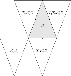
Figure 1. Action of the cusp group on the $\mathbb{C}$-factor of the Heisenberg group $\mathbb{C}\times\mathbb{R}$.

The group $\Gamma_{\infty}$ is actually generated by $T_{1},T_{\tau}$ and $R$, see [15] for instance (note that $T_{v}=[T_{\tau},T_{1}]$). Since $T_{v}$ acts as a translation by $2\sqrt{7}$ in the $t$-coordinate, it should be quite clear that the prism $P=D\times[0,2\sqrt{7}]$ is a fundamental domain for the action of $\Gamma_{\infty}$ in $\mathbb{C}\times\mathbb{R}$, see Figure 2.

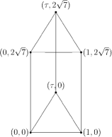
Figure 2. $P=D\times[0,2\sqrt{7}]$ is a fundamental domain for the action of $\Gamma_{\infty}$ on $\mathbb{C}\times\mathbb{R}$

Note that $T_{\tau}R$ and $T_{1}T_{\tau}R$ are side-pairing maps for $P$ (in fact these are complex reflections), and $T_{v}$ as well (it gives the vertical translation pairing the top and bottom triangles of the prism). However $T_{1}R$ is not a side pairing-map (it is given by a glide-reflection), but this will be inconsequential in the present paper.

The domain $P$ is chosen to have affine sides in Heisenberg coordinates (since the Heisenberg group acts on itself by affine transformations, see formula (3)). It can also be adjusted to have well-defined side-pairing maps (this requires subdividing its sides into smaller polygons), but we will not do this, since we do not need it for any of the methods used in this paper.

A few Ford domains in $H^{2}_{\mathbb{C}}$ have been studied explicitly, see [3], [14] among others. Such domains are virtually present in [18] and [13], but it is very complicated to determine their combinatorial structure in detail (or even to describe it on paper!)

To give a rough idea, pictures of (representatives of the isometry type of) the sides of the Ford domain for $\Gamma=U(J,\mathcal{O}_{7})$ are given in Figure 3. Needless to say, these pictures will not be used anywhere in the paper, but they should give an idea of the intricacy of the combinatorics.

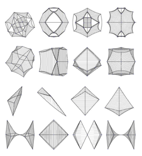
Figure 3. Sides of the Ford domain for $PU(J,\mathcal{O}_{7})$ (four views for each side).

3. Virtual fundamental domain, algorithms

Recall that a coarse fundamental domain for a discrete group $\Gamma$ is a set $\Omega$ such that $\Gamma\Omega=X$, and such that $T=\{\gamma\in\Gamma:\Omega\cap\gamma\Omega\neq\emptyset\}$ is finite. In that case, one can prove that $T$ generates $\Gamma$, and write a explicit group presentation in terms of these generators (see section 13.4 in [11]).

Of course a fundamental domain is a coarse fundamental domain, and this is the kind of coarse fundamental domain we will (virtually) use in this paper. Specifically, we will use $\Omega=F_{\Gamma}\cap C_{P}$, where $C_{P}$ is the cone to the point at infinity in horospherical coordinates, and $P$ is the prism described in [13], i.e.

$$\Omega=\left\{(a+b\tau,t)\ :0\leq a,b,a+b\leq 1,\ 0\leq t\leq 2\right\}.$$

By making virtual use of this domain, we mean that, rather than studying the combinatorics of $\Omega$, we will only use algorithmic procedures that allow us to do the following.

Method 3.1.

1. Determine whether a given algebraic point $[x]\in H^{2}_{\mathbb{C}}$ is inside $\Omega$, and list the sides of $\Omega$ that contain it;

2. If $[x]$ is not in $\Omega$, find an element $\gamma\in\Gamma$ such that $\gamma[x]\in\Omega$.

By an algebraic point $[x]\in H^{2}_{\mathbb{C}}$, we mean a point that can be represented in homogeneous coordinates by a vector $x\in\mathbb{C}^{3}$ with algebraic coordinates. Most algebraic points we consider are actually $\mathbb{K}$-rational (i.e they are represented by a vector in $\mathbb{K}^{3}$), but not all; indeed, the isolated fixed points of a regular elliptic isometry is an eigenvector of a matrix with entries in $\mathbb{K}$, but their eigenvalue need not be in $\mathbb{K}$ in general.

We briefly explain why such methods can be implemented effectively. The main difficulty is that $[x]\in\Omega$ is defined in terms of an infinite set of inequalities.

We first make use of some results in [13], which allow us to reduce the list of $\gamma\in\Gamma$ that occur definition (2.1). This reduction is based on arithmetic considerations.

Here an in what follows, we write $\mathbb{K}=\mathbb{Q}(i\sqrt{7})$, and $\mathcal{O}_{7}$ for the ring of algebraic integers in $\mathbb{K}$.

Definition 3.1.

A $\mathbb{K}$-rational point in $P^{2}_{\mathbb{C}}$ is a point that can be represented in homogeneous coordinates as a vector with entries in $\mathcal{O}_{7}$.

A given a rational point has an essentially unique primitive representative in $\mathcal{O}_{7}^{3}$, i.e. a vector whose entries have greatest common divisor equal to 1 (see Lemma 1 of [13] or Lemma 3 of [16]). The only freedom we have to change such a vector is to scale it by unit, and the only units in $\mathcal{O}_{7}$ are $\pm 1$.

By the square norm of a point in $P^{2} \mathbb{C}$, we mean $||v||^{2}=v^{*}Jv$ for any primitive representative $v\in\mathcal{O}_{7}^{3}$. Points (resp. vectors) with square norm 0 are called null points (resp. vectors). We will use the following result (see Lemma 2 in [13]).

Proposition 3.1.

For every $A\in U(J,\mathcal{O}_{7})$, the first column of $A$ (which represents $A(\infty)$) is a primitive null vector in $\mathcal{O}_{7}^{3}$. Conversely, given any primitive null vector $v\in\mathcal{O}_{7}^{3}$, there exists an $A\in U(J,\mathcal{O}_{7})$ whose first column is $v$.

The converse direction says that the Picard group $\Gamma=U(J,\mathcal{O}_{7})$ acts transitively on $\mathbb{K}$-rational null vectors; this is can be seen as a reformulation of the statement that the quotient $X/\Gamma$ has exactly one cusp, which is a consequence of the fact that $\mathbb{K}$ has class number 1 (see [19] or section 4.1 in [17]). The theoretical result in Proposition 3.1 is unfortunately difficult to make effective, as discussed in [13].

We review the following definition (see [13]).

Definition 3.2.

1. The depth of a $\mathbb{K}$-rational point $[v]\in\partial_{\infty}H^{2}\mathbb{C}\setminus\{\infty\}$ is given by $|v_{3}|^{2}$, where $v=(v_{1},v_{2},v_{3})$ is any primitive integral representative of $[v]$.

2. The depth of a matrix $A\in\Gamma\setminus\Gamma_{\infty}$ is the depth of $A(\infty)$.

The notion of depth is important, in part because of the following Proposition (see Proposition 4.3 of [12]).

Proposition 3.2.

Let $A\in\Gamma$. Then the Cygan center of the isometric sphere $I(A)$ is represented by $A(\infty)$, and its radius is given by $\sqrt{2/d}$, where $d$ is the depth of $A$.

Note that the depth of any $A\in\Gamma$ is a rational integer, but not every integer occurs as the depth of an element $A\in\Gamma$ (only integers that are norms in $\mathcal{O}_{7}$ occur). For example, the first five numbers that occur as depths of elements in the Picard group $\Gamma$ are $1,2,4,7,11$.

If there exists an element of a given depth, then there exist infinitely many, since pre- or post-composition with any element of $\Gamma_{\infty}$ does not change the height. However, in a fixed bounded region of the Heisenberg group $\mathbb{C}\times\mathbb{R}\simeq\partial_{\infty}H^{2}_{\mathbb{C}}\setminus\{\infty\}$, there are only finitely many points of a given depth. This is true in particular in our fundamental domain $P$ for the action of $\Gamma_{\infty}$. A list of $\mathbb{K}$-rational points of small depth in $P$ is given in  [13].

The following result is a consequence of the covering depth estimate given in [13].

Theorem 3.1.

The isometric spheres of elements of depth $\geq 11$ do not intersect the Ford domain $F_{\Gamma}$.

Remark 3.1.

It turns out that the isometric spheres of the elements of depth 7 do intersect the Ford domain, but in lower-dimensional facets only, i.e. they are not needed in the definition (2.1). This fact is quite painful to prove however, and we will not use it in the sequel.

We will also use the following list of 14 elements in the group, which is a slight modification of the list given in [13] (we want the set of side pairing maps to be closed under inversion of matrices).

$$\begin{array}[]{c}A_{1}=\left(\begin{matrix}0&0&1\\ 0&-1&0\\ 1&0&0\end{matrix}\right),\quad A_{2}=\left(\begin{matrix}2&-\tau&1-3\tau\\ \bar{\tau}&0&-2-\tau\\ -\tau&-1&-3+\tau\end{matrix}\right),\quad A_{3}=A_{2}^{-1},\quad A_{4}=A_{2}^{-2},\quad A_{5}=A_{4}^{-1}\\ A_{6}=\left(\begin{matrix}i\sqrt{7}&0&4\\ 0&1&0\\ 2&0&-i\sqrt{7}\end{matrix}\right),\quad A_{7}=\left(\begin{matrix}-\bar{\tau}&1&1\\ \tau&0&1\\ 2&\bar{\tau}&-\tau\end{matrix}\right),\quad A_{8}=\left(\begin{matrix}1&2-\tau&-2\\ -1-\tau&-3&1+\tau\\ -2&-2+\tau&1\end{matrix}\right),\\ A_{9}=\left(\begin{matrix}-1&0&i\sqrt{7}\\ 0&1&0\\ i\sqrt{7}&0&6\end{matrix}\right),\quad A_{10}=\left(\begin{matrix}-2&0&i\sqrt{7}\\ 0&1&0\\ i\sqrt{7}&0&3\end{matrix}\right),\quad A_{11}=A_{10}^{-1},\\ A_{12}=\left(\begin{matrix}-4&0&3i\sqrt{7}\\ 0&1&0\\ i\sqrt{7}&0&5\end{matrix}\right),\quad A_{13}=A_{12}^{-1},\quad A_{14}=A_{9}^{-1}\end{array}$$

The basic fact we will use from [13] is the following.

Theorem 3.2.

Let $\gamma\in\Gamma\setminus\Gamma_{\infty}$ be such that $I(\gamma)$ intersects the Ford domain. Then there exists $\alpha,\beta\in\Gamma_{\infty}$ and $j\in\{1,\dots,14\}$ such that $\gamma=\alpha A_{j}\beta^{-1}$.

The remaining difficulty is that $\Gamma_{\infty}$ is an infinite group, and we cannot check infinitely many inequalities with a computer; we now explain how to handle this difficulty.

In sections 3.1 through 3.4, we sketch the general algorithms we will use. We then list the specific results (conjugacy classes of torsion elements, maximal finite subgroups) for the group $U(J,\mathcal{O}_{7})$ in section 4.

3.1. Basic algorithms

Recall that we are after algorithmic methods stated in Method 3.1. Let us assume $x\in\mathbb{C}^{3}$ has algebraic coordinates, and $||x||^{2}<0$. We can compute the (algebraic) horospherical coordinates $(z,t,u)$ of $x$, using

$$z=\frac{x_{2}}{x_{3}},it-u=2\frac{x_{1}}{x_{3}}+|\frac{x_{2}}{x_{3}}|^{2}.$$

We would like to find a cusp element $\gamma\in\Gamma_{\infty}$ such that $\gamma(x)$ has horospherical coordinates $(z^{\prime},t^{\prime},u^{\prime})$ with $(z^{\prime},t^{\prime})\in P$. Recall that $P\subset\mathbb{C}\times\mathbb{R}$ is $T\times[0,2\sqrt{7}]$ where $T$ is the convex hull of $0,1$ and $\tau$.

First solve

$$a+b\tau=z\leftrightarrow\left\{\begin{array}[]{l}a+\frac{b}{2}=\textrm{Re}(z)\\ b\sqrt{7}=\textrm{Im}(z)\end{array}\right.$$

for real algebraic $a,b$, and compute the floors $k=\lfloor a\rfloor$ and $l=\lfloor b\rfloor$, $\epsilon=\lfloor a+b\rfloor$. By applying $T_{1}^{-k}T_{\tau}^{-l}$ for suitably chosen $k,l\in\mathbb{Z}$, we may assume the horospherical coordinates $(z,t,u)$ satisfy $z\in T$. Computing $\lfloor t/(2\sqrt{7})\rfloor$, we get a power of $T_{v}$ that brings the $t$-coordinate in $[0,2\sqrt{7}]$.

In other words, we may assume that $(z,t)\in P$. Now we use the following.

Proposition 3.3.

Let $j\in\{1,\dots,14\}$. There is an explicit set $E_{j}\subset\Gamma_{\infty}$ such that for all $\gamma\in\Gamma_{\infty}\setminus E_{j}$, we have $\gamma(I(A_{j}))\cap C_{P}=\emptyset$.

Without the “explicit” request, this is a consequence of discreteness of $\Gamma_{\infty}$. The explicit character follows from elementary estimates using the values of the Cygan radius of $I(A_{j})$ (for details on these estimates, see [5]).

Using Proposition 3.3, we can list all the isometric spheres $\alpha(I(A_{j}))$ that contain $[x]$ (or such that $[x]$ is in the interior of the corresponding Cygan ball). This gives method (1).

For method (2), we first proceed as above to bring the Heisenberg coordinate to $P$, then find the Cygan spheres $\alpha(I(A_{j}))$ that contain $x$, and apply the isometry $(\alpha A_{j})^{-1}$ to $x$. This decreases the number of Cygan balls defining the Ford domain that contain $[x]$ in their interior. Then repeat the preceding procedure until that number is 0.

3.2. Conjugacy classes of torsion elements

Clearly every torsion element is conjugate to a torsion element that fixes a point in the fundamental domain $\Omega=F_{\Gamma}\cap C_{P}$. Moreover, the dicreteness of $\Gamma$ implies that there exists a precisely invariant horoball, i.e. a horoball $B$ based at $q_{\infty}$ such that is invariant under $\Gamma_{\infty}$, and $\gamma(B)\cap B=\emptyset$ for every $\gamma\in\Gamma\setminus\Gamma_{\infty}$. Moreove, the fact that $\Gamma$ is a lattice implies that $\Gamma_{\infty}$ acts cocompactly on every horosphere based at $q_{\infty}$.

It follows that there are actually finitely many torsion elements fixing a point in $\Omega$; we now explain a method for listing these elements.

Suppose $\gamma\in\Gamma$ has finite order. There are two possibilities, either $\gamma\in\Gamma_{\infty}$ or not.

3.2.1. $\gamma\in\Gamma_{\infty}$

In this case, $\gamma$ must be a complex reflection, and we may assume that its mirror meets the Heisenberg group $\mathbb{C}\times\mathbb{R}$ in a vertical line that intersects the boundary of the prism $P$. Projecting to the $\mathbb{C}$-factor, it is easy to see that the boundary at infinity of the mirror is given by $\{(z_{0},t):t\in\mathbb{R}\}$ for $z_{0}=0$, $1/2$, $\tau/2$, $(1+\tau)/2$. This implies that $\gamma$ has one of the following forms:

$$RT_{v}^{k},\quad T_{1}RT_{v}^{k},\quad T_{\tau}RT_{v}^{k},\quad T_{1}T_{\tau}RT_{v}^{k},$$

for some $k\in\mathbb{Z}$ (we will give more details about this in section 4.1). The only complex reflections of this form are

$$R,T_{1}R,T_{1}T_{\tau}R.$$

3.2.2. $\gamma\notin\Gamma_{\infty}$

Suppose $\gamma$ fixes a point $[x]\in P$. It is easy to see from the definition of isometric spheres that we must have $[x]\in I(\gamma)\cap I(\gamma^{-1})$, and in particular

$$I(\gamma)\cap I(\gamma^{-1})\neq\emptyset.$$

Also, because the fixed point $[x]$ is in the Ford domain, $\gamma$ must have depth $\leq 7$, so $\gamma=\alpha A_{j}\beta^{-1}$ for some $j\in\{1,\dots,14\}$ and $\alpha,\beta\in\Gamma_{\infty}$ (see Theorem 3.2).

Since we only want to list torsion elements up to conjugacy, we may assume $\beta=Id$, i.e. $\gamma=\alpha A_{j}$, and we get

$$\emptyset\neq I(\gamma)\cap I(\gamma^{-1})=\alpha(I(A_{j}))\cap I(A_{j}^{-1}).$$

Note that we chose the set $\{A_{1},\dots,A_{14}\}$ to be invariant under the operation of taking inverses, so there is a $k\in\{1,\dots,14\}$ such that $I(A_{j}^{-1})=I(A_{k})$, and we must have

$$\alpha(I(A_{j}))\cap A_{k}\neq\emptyset.$$

Proposition 3.4.

There is an explicit finite set $T_{jk}$ such that for all $\alpha\in\Gamma_{\infty}\setminus T_{jk}$, $\alpha(I(A_{j}))\cap A_{k}=\emptyset$.

The set can be made explicit by using elementary estimates using the triangle inequality and the known radii of the Cygan spheres $I(A_{j})$, $I(A_{k})$ (see equation (6)). For more details, see [5].

From this, we get that every torsion element in $\Gamma\setminus\Gamma_{\infty}$ is conjugate to an element of the finite sets $T_{jk}$ for $j,k\in\{1,\dots,14\}$ (and we may restrict to pairs $j,k$ such that $A_{j}A_{k}=Id$).

Moreover, given an element $\gamma\in T_{jk}$, there is an algorithm to determine whether $\gamma$ has finite order. Indeed, the eigenvalues of the matrix representative for $\gamma$ (which is unique up to multiplication by $-Id$) are algebraic integers, and we can determine whether they are roots of unity by examining their minimal polynomial.

If the eigenvalues are all roots of unity, we can check whether or not the matrix is diagonalizable by computing its minimal polynomial. Hence we have an algorithm to do the following.

Method 3.2.

Produce a finite set that contains a representative of every conjugacy class of torsion element in $\Gamma$.

For elements with isolated fixed points, we can use methods of section 3.1, we remove all elements whose fixed point set is not in the fundamental domain $\Omega$, since they must be conjugate to another element in the list.

3.3. Eliminating redundancy

The list obtained by applying the method explained in section 3.2 may have redundancies, in the sense that some elements in the list may be conjugate to each other.

We now explain how to test whether two torsion elements $\gamma_{1}$, $\gamma_{2}$ are conjugate to each other, assuming that they both have an isolated fixed point. We call $x_{j}$ the isolated fixed point of $\gamma_{j}$; by the methods of section 3.1, we may assume $x_{1},x_{2}$ are both in $\Omega$.

Suppose $\gamma_{1},\gamma_{2}$ are conjugate in $\Gamma$, i.e there exists $\alpha\in\Gamma$ such that $\gamma_{2}=\alpha\gamma_{1}\alpha^{-1}$. Then $\alpha(x_{1})=x_{2}$, and in particular

$$\Omega\cap\alpha(\Omega)\neq\emptyset.$$

This implies that for some $j\in\{1,\dots,14\}$, $\alpha(I(A_{j}))$ must intersect $P$, and there are finitely many choices of $\alpha$ such that this is the case (as before, this can be made explicit).

Hence we only need to check finitely candidate conjugators $\alpha$ in order to determine whether the two elements are conjugate, making this special case of the conjugation problem solvable.

For pairs of complex reflections, it is more complicated to write a general algorithm to test conjugacy (because the stabilizer of the mirror of one such complex reflection is infinite). In order to treat the special case of $PU(J,\mathcal{O}_{7})$, it suffices to use the following two observations

1. It two elements are conjugate, then we can find an element that conjugates them by listing all group elements, by listing words in a fixed generating set in increasing word length;

2. If two complex reflections have different order, or different Jordan forms, or different square norm for their (primitive) polar vector, then they are not conjugate.

For a general group, we are likely to find pairs of elements with the same rough conjugacy invariants (order, Jordan form, square norm of polar vector) but the enumeration of the group fails finding a conjugator (say because we run out of time or memory).

3.4. Finding maximal finite subgroups

In this section, we explain how to determine maximal finite subgroups. We assume that we have applied the methods of section 3 successfully, and that we have a finite list of all torsion elements whose fixed points contain a point in $\Omega$.

The interesting maximal finite subgroups contain an element with an isolated fixed point, since generic points on the mirror of a complex reflection have a cyclic group as their stabilizer, generated by a single complex reflection.

Now take the list of torsion elements with an isolated fixed point in $\Omega$. For each such fixed point $[x]$, we use the methods of section 3.1 to find the list of Ford spheres and sides of $C_{P}$ containing $[x]$.

Now build a graph whose vertex set is in bijection with the set of these isolated fixed points, and join two vertices by a directed edge if there is a side-pairing map sending one to the other (either coming from the Ford domain, or from the prism $P$); note that the edges may join a vertex to itself.

The conjugacy classes of maximal finite groups in $\Gamma$ are then given by connected component of this graph (take the image of the obvious representation of the fundamental group of the graph into $\Gamma$).

For concreteness, we work out a couple of explicit examples.

1. Consider $M=(RT_{1}IT_{1}^{-1})^{2}$ for instance (see the first entry in Table 2). Its isolated fixed point is given by $[v_{1}]$ where $v_{1}=(-\bar{\tau},0,1)$, which has horospherical coordinates $[0,\sqrt{7},1]$. This point is on two sides of the cone $C_{P}$ (namely the ones with side-pairing $T_{\tau}R$ and $T_{1}R$), as well as on three Ford-Cygan spheres , namely

   $$I(A_{6}),T_{1}(I(A_{1})),T_{1}^{-1}T_{v}(I(A_{1})).$$

   The side-pairing maps associated to these sides are given respectively by

   $$A_{6},T_{1}A_{1}T_{1}^{-1},T_{1}^{-1}T_{v}A_{1}T_{v}^{-1}T_{1},$$

   and each of these elements actually fixes $[v]$.

   Using the side-pairings coming from $C_{P}$, we find two other points $[v_{2}]$, $[v_{3}]$ given $v_{2}=T\tau Rv_{1}$ and $v_{3}=T_{1}Rv_{1}$. Each is on three Ford-Cygan spheres, which are simply the images of the above three Cygan spheres under $T_{\tau}R$ (or $T_{1}R$).

   Hence the connected component of the graph containing $[v_{1}]$ is a triangle as in Figure 4. The stabilizer of $[v_{1}]$ is generated by $A_{6},T_{1}A_{1}T_{1}^{-1},T_{1}^{-1}T_{v}A_{1}T_{v}^{-1}T_{1}$ together with the element

   $$(T_{1}R)^{-1}T_{1}T_{\tau}RT_{\tau}R=R.$$

   

   Figure 4. Cycle graph for the vertex $v_{1}$. We omit the Ford side-pairing maps that fix $v_{2}$ (resp. $v_{3}$), since these are simply conjugates of the elements in the label for the loop from $v_{1}$ to itself.

   The linear group generated by $R,A_{6},T_{1}A_{1}T_{1}^{-1},T_{1}^{-1}T_{v}A_{1}T_{v}^{-1}T_{1}$ has order 16, and its subgroup of scalar matrices has order 2. In other words, the stabilizer of $[v_{1}]$ in $\Gamma$ has order 8.

   It is easy to check (for instance by enumerating the elements in the stabilizer) that the stabilizer contains four complex reflections.

   Let us denote $v_{1},\dots,v_{4}$ polar vectors to the mirrors of these reflections, which we may and do chose to be primitive vectors in $\mathcal{O}_{7}^{3}$. Explicit computation shows that, perhaps after permuting these vectors, we have $\langle v_{1},v_{1}\rangle=\langle v_{2},v_{2}\rangle=1$, $\langle v_{1},v_{1}\rangle=\langle v_{2},v_{2}\rangle=2$.

   This kind of information is gathered in columns 4 through 6 of Tables 2-6 (see also Definition 4.1).

2. Consider the element $N=(T_{\tau}R)\cdot T_{1}R(T_{1}I)^{2}T_{1}^{-1}RT_{1}IT_{1}^{-1}\cdot(RT_{\tau}^{-1})$, which is the element of order 6 given in Table 5, conjugated by $T_{\tau}R$ so that its isolated fixed point $[w]$ is in $\Omega$.

   The corresponding point is not on any side of the cone $C_{P}$, but it is on five Ford Cygan spheres, namely

   $$I(A_{2}),I(A_{3}),RT_{\tau}^{-1}(I(A_{4})),RT_{\tau}^{-1}T_{1}^{-1}(I(A_{5})),T_{\tau}(I(A_{6})).$$

   The point $[A_{2}^{-1}w]$ is inside the Ford domain, but it is not in the cone $C_{P}$, so we bring it back to the cone by a cusp element. It turns out $T_{\tau}R$ does the job, i.e. $T_{\tau}RA_{2}^{-1}w\in\Omega$. Note that the Cygan sphere for $(T_{\tau}RA_{2}^{-1})^{-1}=A_{2}\cdot RT_{\tau}^{-1}$ is of course the same as the one for $A_{2}$, since these two elements differ by pre-composition by a cusp element.

   Similar considerations show that (adjusted) side-pairing maps corresponding to the above five Cygan spheres are

   $$\begin{array}[]{c}T_{\tau}R\cdot A_{2}^{-1},\\ T_{1}T_{\tau}R\cdot A_{3}^{-1},\\ T_{\tau}^{2}R\cdot(T_{\tau}A_{6}^{-1}T_{\tau}^{-1}),\\ T_{1}\cdot(RT_{\tau}^{-1}A_{4}^{-1}T_{\tau}R),\\ T_{1}^{-1}\cdot(RT_{\tau}^{-1}T_{1}^{-1}A_{5}^{-1}T_{1}T_{\tau}R)\\ \end{array}$$

   and all these elements fix $[w]$. In other words, the relevant (connected component of the) cycle graph has a single vertex, and 5 loops.

   The above five matrices generate a linear group of order 12, whose projectivization is a cyclic group of order 6. There is a complex reflection in this group, obtained by taking the third power of a generator (see Table 5).

4. Results

4.1. Torsion in $\Gamma_{\infty}$

We first consider cusp elements. Suppose $\gamma\in\Gamma_{\infty}$ and $\gamma(\Omega)\cap\Omega\neq\emptyset$. Then $\gamma(P)\cap P\neq\emptyset$. Looking at the first component in Heisenberg space $\mathbb{C}\times\mathbb{R}$, we easily find neighboring triangles in the tiling, which are obtained by applying elements of the form

$$\gamma=T_{1}^{j}T_{\tau}^{k}(T_{1}T_{\tau}R)^{\epsilon}T_{v}^{l},$$

with $-1,\leq j,k,j+k\leq 1$, $\epsilon=0$ or $1$. A picture of the corresponding tiling is given in Figure 5.

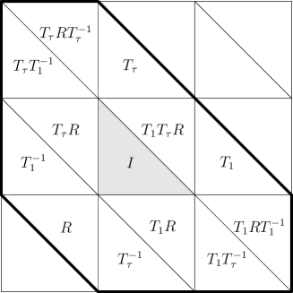
Figure 5. Horizontal tiling in Heisenberg space, using coordinates in the $\mathbb{R}$-basis $1,\tau$

For each such element, it is easy to check which values of $l$ give $\gamma(P)\cap P\neq\emptyset$ (in all cases $-1\leq l\leq 1$ is necessary).

Checking the corresponding elements, we find that the only cusp elements in $T$ (see equation 2) are

$$R,T_{1}RT_{1}^{-1},T_{\tau}RT_{\tau}^{-1},T_{\tau}R,T_{1}T_{\tau}R,$$

each of order 2.

We will shortly see that $T_{\tau}R$ and $T_{1}T_{\tau}R$ are conjugate in $\Gamma$, but they are not conjugate to $R$. In particular, we have (1) in the following.

Proposition 4.1.

Let $\gamma\in\Gamma_{\infty}$.

1. If $\gamma$ is a non-trivial torsion element, then it is conjugate in $\Gamma$ to $R$ or to $T\tau R$.

2. If $\gamma$ is parabolic but not unipotent, then it is conjugate in $\Gamma$ to $T_{1}RT_{v}^{k}$, $RT_{v}^{k}$ or $T_{\tau}RT_{v}^{k}$ for some $k\in\mathbb{Z}$.

Point (2) follows from the fact that the prism is a fundamental domain for the action of $\Gamma_{\infty}$ in Heisenberg space. Indeed, invariant complex lines for non-unipotent cusp elements can be assumed to meet the boundary at infinity in one of the four vertical lines $(0,t)$, $(\frac{1}{2},t)$, $(\frac{\tau}{2},t)$, $(\frac{1+\tau}{2},t)$ in Heisenberg. The last two are conjugate in $\Gamma$ (but the first three have distinct conjugacy classes in $\Gamma_{\infty}$).

Since our method is not algorithmic for complex reflections, we list the conjugations needed in order to show that there are indeed just two conjugacy classes of complex reflections in $\Gamma$ (both of order 2):

(9) $$\begin{array}[]{c}(T_{1}R)^{2}T_{1}^{-1}(T_{\tau}R)((T_{1}R)^{2}T_{1}^{-1})^{-1}=I\\ \ [T_{1},I](T_{\tau}R)[T_{1},I]^{-1}=T_{1}T_{\tau}R\\ \left(\begin{matrix}i\sqrt{7}&0&4\\ 0&-1&0\\ 2&0&-i\sqrt{7}\end{matrix}\right)=T_{1}IT_{1}^{-1}(R)(T_{1}IT_{1})^{-1}.\end{array}$$

The first two equations show that $T_{\tau}R$ and $T_{1}T_{\tau}R$ are both conjugate to $I$. The left hand side of the last equation is one of the complex reflections produced by listing elements of finite order $\gamma$ with $\Omega\cap\gamma\Omega\neq\emptyset$.

4.2. Conjugacy classes of torsion elements

The results below were of course obtained with the help of a computer (using the methods of section 3). After this paper was written, we have developed a computer program that performs this analysis systematically (for general 1-cusped Picard lattices), see [2].

For complex reflections, there are precisely two conjugacy classes, listed in Table 1.

Matrix	Polar to mirror $v$	$\langle v,v\rangle$
$R=\left(\begin{matrix}1&0&0\\ 0&-1&0\\ 0&0&1\end{matrix}\right)$	$(0,1,0)$	$1$
$I=\left(\begin{matrix}0&0&1\\ 0&-1&0\\ 1&0&0\end{matrix}\right)$	$(1,0,1)$	$2$

Table 1. Representatives of conjugacy classes of elements of complex reflections (of order 2) in $PU(2,1,\mathcal{O}_{7})$

Note that the two classes can be distinguished by the square norm of the primitive vector polar to their mirror, which suggests the following definition.

Definition 4.1.

For $j=1,2$, a $j$-line is a complex line polar to a primitive vector $v\in\mathcal{O}_{7}$ such that $\langle v,v\rangle=j$.

The following result follows from the list of conjugacy classes of complex reflections in $\Gamma$ (see Table 1).

Proposition 4.2.

The group $\Gamma$ acts transitively on the set of primitive vectors of square norm $1$ (resp. $2$) in $\mathcal{O}_{K}^{3}$.

Proof: To each $j$-line ($j=1$ or $2$) polar to $v$, the associated complex reflection is indeed in $U(J,\mathcal{O}_{7})$, since it is given by

(10) $$R_{v}(x)=x-2\frac{\langle x,v\rangle}{\langle v,v\rangle}v,$$

and $\langle v,v\rangle$ divides 2. The transitivity now follows from the fact that there are exactly two conjugacy classes of complex reflections in $\Gamma$. $\Box$

We list the conjugacy classes of torsion elements with isolated fixed points in Tables 2 through 6. For each class, we give the norm of a primitive vectors representing the fixed point. We also list the order of the stabilizer of the fixed point (obtained with the method explained in section 3.4), as well as the number of 1-lines and 2-lines through that point, see Definition 4.1. Recall that being a 1-line (resp. 2-line) is equivalent to being in the $\Gamma$-orbit of the mirror of $R$ (resp. of $I$).

Matrix	Fixed pt $v$	$\langle v,v\rangle$	$|Stab|$	1-lines	2-lines
$(RT_{1}IT_{1}^{-1})^{2}=\left(\begin{matrix}i\sqrt{7}&0&4\\ 0&1&0\\ 2&0&-i\sqrt{7}\end{matrix}\right)$	$(-\bar{\tau},0,1)$	$-1$	8	2	2
$IR=\left(\begin{matrix}0&0&1\\ 0&1&0\\ 1&0&0\end{matrix}\right)$	$(-1,0,1)$	$-2$	4	1	1
$T_{1}^{2}I(T_{1}^{-1}I)^{2}T_{1}^{2}I=\left(\begin{matrix}-\bar{\tau}&\tau&2\\ \tau&2&\bar{\tau}\\ 2&\bar{\tau}&-\tau\end{matrix}\right)$	$(\tau,1,\bar{\tau})$	$-2$	8	0	4

Table 2. Representatives of conjugacy classes of elements of order 2 with an isolated fixed point in $PU(2,1,\mathcal{O}_{7})$

Matrix	Fixed pt $v$	$\langle v,v\rangle$	$|Stab|$	1-lines	2-lines
$T_{1}(IT_{1}^{-1})^{2}(IT_{1})^{2}=\left(\begin{matrix}-1&\tau&1\\ -\bar{\tau}&1&0\\ 1&0&0\end{matrix}\right)$	$(\tau,1,-\tau)$	$-3$	6	0	3
$T_{1}^{2}(IT_{1}^{-1})^{2}(IT_{1})^{2}=\left(\begin{matrix}-1&-\bar{\tau}&1\\ \tau&1&0\\ 1&0&0\end{matrix}\right)$	$(-\bar{\tau},1,\bar{\tau})$	$-3$	6	0	3
$(RT_{1})^{2}IT_{1}IT_{1}^{-1}RT_{1}IT_{1}^{-1}=\left(\begin{matrix}5&0&-3i\sqrt{7}\\ 0&-1&0\\ -i\sqrt{7}&0&-4\end{matrix}\right)$	$\notin\mathbb{K}^{3}$		6	1	0

Table 3. Representatives of conjugacy classes of elements of order 3 (isolated fixed point) in $PU(2,1,\mathcal{O}_{7})$

Matrix	Fixed pt $v$	$\langle v,v\rangle$	$|Stab|$	1-lines	2-lines
$IT_{1}^{-1}RT_{1}=\left(\begin{matrix}0&0&1\\ 0&1&2\\ 1&-2&-2\end{matrix}\right)$	$(-1,-1,1)$	$-1$	8	2	2
$(T_{1}^{-1}I)^{2}(T_{1}I)^{2}=\left(\begin{matrix}0&0&1\\ 0&1&1+\bar{\tau}\\ 1&-1-\tau&-2\end{matrix}\right)$	$(\bar{\tau},-\tau,-\bar{\tau})$	$-2$	8	0	2+2

Table 4. Representatives of conjugacy classes of elements of order 4 (isolated fixed point) in $PU(2,1,\mathcal{O}_{7})$. The occurrence of $2+2$ in the last column means that there are four $2$-lines through the fixed point, that come in two distinct orbits under the action of the stabilizer.

Matrix	Fixed pt $v$	$|Stab|$	1-lines	2-lines
$T_{1}R(T_{1}I)^{2}T_{1}^{-1}RT_{1}IT_{1}^{-1}=\left(\begin{matrix}-5&0&3i\sqrt{7}\\ 0&-1&0\\ i\sqrt{7}&0&4\end{matrix}\right)$	$\notin\mathbb{K}^{3}$	6	1	0

Table 5. Representatives of conjugacy classes of elements of order 6 (isolated fixed point) in $PU(2,1,\mathcal{O}_{7})$

Matrix	Fixed pt $v$	$|Stab|$	1-lines	2-lines
$IRT_{1}=\left(\begin{matrix}0&0&1\\ 0&1&1\\ 1&-1&-\bar{\tau}\end{matrix}\right)$	$\notin\mathbb{K}^{3}$	7	0	0

Table 6. Representatives of conjugacy classes of elements of order 7 (isolated fixed point) in $PU(2,1,\mathcal{O}_{7})$

5. Study of the mirror stabilizers

5.1. Mirror of $R$

The mirror of $R$ is given by the complex lines in $e_{2}^{\perp}$, so it is quite clear that its stabilizer is isomorphic to $\{\pm 1\}\times U(1,1,\mathcal{O}_{7})$. In terms of our standard horospherical coordinates $(z,t,u)$, the mirror is simply given by the points with $z=0$, i.e. we get a copy of the upper half space $(t,u)\in\mathbb{R}^{2}$, $u>0$.

The stabilizer can be understood with the same method as in [13], only the computations are simpler. Concretely, to work out the Ford domain for the stabilizer, we restrict to $z=0$ and consider the domain bounded by Cygan spheres for elements $\gamma\in\Gamma$ only when $\gamma$ preserves $z=0$ (this last is equivalent to saying that its matrix representative should have $(1,0,0)$ as an eigenvector, and it implies that $\gamma(\infty)$ have 0 as its second homogeneous coordinate). Of course there are infinitely many such elements, but up to the action of $\Gamma_{\infty}$, the points $\gamma(\infty)$ must be the ones listed in [13].

Also, the cusp elements that preserve $z=0$ consists precisely of elements in the infinite cyclic group generated by the vertical translation $T_{v}$.

It turns out that, up to the action of the group generated by $T_{v}$, there is a unique element of depth 1, namely

$$I=\left(\begin{matrix}0&0&1\\ 0&-1&0\\ 1&0&0\end{matrix}\right),$$

and a unique element of depth 2, given by

$$M=\left(\begin{matrix}i\sqrt{7}&0&4\\ 0&1&0\\ 2&0&-i\sqrt{7}\end{matrix}\right).$$

Moreover, the corresponding Cygan spheres intersect at the (isolated) fixed point of

$$MT_{v}I,$$

which has order 6 (its cube is actually equal to $R$, so the transformation acts as an element of order 3 in restriction to the mirror of $R$).

It follows from the results in [13] that the Cygan spheres of level 11 or higher do not intersect the Ford domain, so the determination of the Ford domain for the stabilizer is reduced to finitely many verifications, and one verifies that the $T_{v}$-translates of the two Cygan spheres for $I$ and $M$ actually bound the domain, and that a fundamental domain for the action of the stabilizer is as illustrated in Figure 6.

Figure 6. Fundamental domain with side-pairing for the action of the stabilizer of the mirror of $R$.

It is also easy to work out the vertex cycles of the corresponding Ford polygon, to get a presentation for the fixed point stabilizer of the form

$$\langle\iota,\mu,\upsilon|\iota^{2},\mu^{2},(\mu\upsilon\iota)^{3}\rangle.$$

The stabilizer is a central extension of this group with presentation

$$\langle\iota,\mu,\upsilon,\rho|\iota^{2},\mu^{2},\rho^{2},(\mu\upsilon\iota)^{3}\rho^{-1},[\rho,\iota],[\rho,\mu],[\rho,\upsilon]\rangle.$$

The above discussion shows in particular that the mirror stabilizer has precisely three orbits of points with non-trivial isotropy groups, represented by

• The common fixed point of $I$ and $R$ (intersection of one 1-line and one 2-line)

• The fixed point of $(RT_{1}IT_{1}^{-1})^{2}$ (intersection of two 1-lines and two 2-lines)

• The fixed point of $MT_{v}I$ (only one 1-line).

5.2. Mirror of $I$

Instead of considering the stabilizer of the mirror of $I$, we will study the mirror of $T_{\tau}R$ (which is conjugate to $I$ in $\Gamma$), because its mirror goes through the point at infinity in the Siegel half space.

Let $L$ be the mirror of $T_{\tau}R$, which is given by $v^{\perp}$ with $v=(1,-\tau,0)$. The structure of the stabilizer of $L$ in $\Gamma$ is significantly more difficult to study. Our main result is the following.

Theorem 5.1.

The projection of the stabilizer of $L$ to $PU(1,1)$ is the lattice generated by seven elements $r_{1},r_{2},r_{3},r_{4}$, $s_{1},s_{2}$, with presentation

(11) $$\langle r_{1},r_{2},r_{3},r_{4},s_{1},s_{2},t_{v}\ |\ r_{1}^{2},r_{2}^{3},r_{3}^{2},r_{4}^{2},(s_{2}^{-1}s_{1})^{2},s_{1}^{-1}r_{4}r_{1}r_{3}t_{v}r_{2}\ \rangle.$$

This group has precisely two cusps, corresponding to the cyclic groups generated by $t_{v}$ and $s_{2}$. The image of the mirror in the quotient is a $P^{1}_{\mathbb{C}}$ with 2 punctures and 4 orbifold points of weight 2.

Just as in section 5.1, $Stab(L)$ is in fact a central extension of this group, with center generated by the complex reflection $T_{\tau}R$ itself (which acts trivially on $L$).

We obtained this group by using the computer to list many primitive vectors $v\in\mathcal{O}_{7}^{3}$ with norm 1 or 2, and keeping only those that are orthogonal to $v=(1,-\tau,0)$ (so that the corresponding complex reflections $R_{v}$ preserves $L$). We then studied the Ford domain (see Figure 7) for the group generated by those reflections, whose side-pairing maps are the above generators.

The group elements $r_{1},\dots,r_{4}$ are complex reflections with mirror a $2$-line. We describe them by giving vectors $v_{1},\dots,v_{4}$ polar to their mirror; recall that the matrix of the reflection $R_{v}$ fixing $v^{\perp}$ can be obtained by using formula (10).

(12) $$\begin{array}[]{c}v_{1}=(1,1,\bar{\tau})\\ v_{2}=(-i\sqrt{7},\tau,2)\\ v_{3}=(i\sqrt{7},\tau,2)\\ v_{4}=(0,1,\bar{\tau}).\end{array}$$

For the other two, we give the full matrices, namely

(13) $$s_{1}=\left(\begin{matrix}-\tau-1&\tau-2&\bar{\tau}+2\\ 3\tau&4&-5\\ 6&3\bar{\tau}&5\tau-4\end{matrix}\right),\quad s_{2}=\left(\begin{matrix}\tau-3&i\sqrt{7}&-i\sqrt{7}\\ \bar{\tau}+3&1-i\sqrt{7}&i\sqrt{7}\\ -2i\sqrt{7}&-\tau-3&\tau+4\end{matrix}\right).$$

It is easy to check that $s_{2}$ is a parabolic element, whose fixed point is represented by the primitive vector $(-1,1,\bar{\tau})$.

A fundamental domain for the action of the stabilizer of $L$ is described in Figure 7. From this, one easily deduces a presentation of the stabilizer of $L$ (modulo the fixed point stabilizer of $L$, which is a group of order 2), by using the Poincaré polygon theorem. Indeed, the relations that occur in the presentation of equation (11) are the cycle relations coming from the vertices of the fundamental domain.

Figure 7. A fundamental domain for the action in $L$ of $Stab(L)$.

A priori the above group is only the (projection to $PU(1,1)$ of the) subgroup of $Stab(L)$ generated by all the complex reflections in $Stab(L)$, but in fact this gives full stabilizer, because any holomorphic symmetry of our domain would have to exchange the two cusps (but it is easy to see that there is no $A\in U(2,1,\mathcal{O}_{7})$ that exchanges $(1,0,0)$ and $(-1,1,\bar{\tau})$).

6. A 2-generator presentation

Theorem 6.1.

The group $\Gamma_{7}=PU(2,1,\mathcal{O}_{7})$ has the following presentation

$$\langle\ a,b,c,d\ |\ a^{7},b^{2},c^{6},(ad^{2})^{4},(c^{-2}d^{2})^{4},(cd^{-1}c^{2}d^{-2})^{3},(cd^{-2}c^{2}d^{-1})^{3},(d^{2}c^{-1}a^{-2}d^{3}c^{2}a^{-2})^{2},c^{-1}ab,d^{-1}ba\ \rangle$$

Moreover, every torsion element in the group is conjugate to an element that occurs in one of these power relators.

Note that we write this as a 4-generator presentation to help readability, but it should be clear (by looking at the last two relators) that $a,b$ generate the group, and this can clearly be turned into a 2-generator presentation (this is useful to speed up computations using group-theory software like GAP or Magma).

An explicit isomorphism $\phi:G\rightarrow PU(2,1,\mathcal{O}_{7})$ extends $\phi(a)=A$, $\phi(b)=B$ where

$$A=\left(\begin{matrix}-\tau-2&i\sqrt{7}&i\sqrt{7}\\ -1&1&0\\ \tau-1&1&1\end{matrix}\right),\quad B=\left(\begin{matrix}1&\bar{\tau}&-1\\ 0&-1&\tau\\ 0&0&1\end{matrix}\right).$$

The fact that $\phi(a)=A$, $\phi(b)=B$ extends to a group homomorphism (still denoted by $\phi$) follows from explicit matrix computation. The fact that this extension is an isomorphism follows from comparison of $G$ with the presentation for $PU(2,1,\mathcal{O}_{7})$ given in [13] using the SearchForIsomorphism command in Magma.

We would like to find an element of each torsion conjugacy class expressed as an explicit word in $a,b$. We start by gathering geometric data for the obvious elements that occur in the presentation in equation (6.1), see Table 8.

Order	Group element	Fixed point $v$	$\langle v,v\rangle$	Other descr.
2	$b$	$(1,-\tau,0)$	$2$	$T_{\tau}R$
2	$(ba)^{3}=d^{3}=a^{-1}c^{3}a$	$(\tau,0,1)$	$1$	$T_{1}IT_{1}^{-1}RT_{1}IT_{1}^{-1}$
2	$((aba)^{-1}babab)^{2}=(d^{-2}c^{2})^{2}$	$(\tau,1,\bar{\tau})$	$-2$	$\#3$
2	$(ababa)^{2}=(ad^{2})^{2}$	$(\tau+1,1,\bar{\tau})$	$-1$	$A_{2}(\#1)A_{2}^{-1}$
3	$(ba)^{2}=d^{2}$	not in $\mathbb{Q}(i\sqrt{7})$		$T_{1}(IT_{1}^{-1}R)^{3}$
3	$[b,a^{-1}babab]=c^{-1}d^{2}c^{-2}d$	$(3+i\sqrt{7},1,\bar{\tau})$	$-3$	$T_{v}I(T_{\tau}J)ITv^{-1}$
4	$(aba)^{-1}babab=d^{-2}c^{2}$	$(\tau,1,\bar{\tau})$	$-2$	$IT_{1}^{-1}(IT_{1})^{2}IT_{1}^{-1}$
4	$ababa=ad$	$(\tau+1,1,\bar{\tau})$	$-1$	$T_{1}I(T_{1}^{-1}I)^{2}T_{1}IRT_{1}IT_{1}^{-1}$
6	$ab=c$	not in $\mathbb{Q}(i\sqrt{7})$		$RT_{1}IR(T_{1}I)^{2}T_{1}^{-2}$
7	$a$	not in $\mathbb{Q}(i\sqrt{7})$		$T_{1}RT_{1}IRT_{1}I$

Figure 8. Obvious elements of finite order, obtained from the presentation (6.1).

In order to get all torsion conjugacy classes (up to replacing any element to a power that generates the same finite cyclic group), we need to write a conjugate of $IR$ and a conjugate of $T_{\bar{\tau}}^{-1}J$ as explicit words in $a$ and $b$. This can be done using the above explicit isomorphism between the presentations (or alternatively by geometric methods using a suitable Dirichlet domain for the group).

The results are give in Table 9.

Order	Group element	Fixed point $v$	$\langle v,v\rangle$	Other descr.
2	$(aba)^{-1}(d^{2}c^{-1}a^{-2}d^{3}c^{2}a^{-2})aba$	$(1,0,-1)$	$-2$	$J=RI$
3	$a^{-1}ba^{-1}bababa^{-1}bab=d^{-2}c^{2}d^{-1}c$	$(\tau+1,\bar{\tau},-\tau)$	$-3$	$T_{1}I(T_{\bar{\tau}}^{-1}J)IT_{1}^{-1}$

Figure 9. Non-obvious elements of finite order.

7. Torsion-free subgroups

We now use the results of the previous sections to exhibit an explicit torsion-free subgroup of $\Gamma$. Computer code to find this subgroup (as well as many other torsion-free subgroups of $PU(J,\mathcal{O}_{d})$ for other values of $d$) is available in [2].

Recall that $\Gamma$ contains elements of order $2,3,4,6$ and $7$, so the index of any torsion-free subgroup has to be a multiple of $\textrm{lcm}(\{4,6,7\})=84$.

Consider the ideal $I=\langle i\sqrt{7}\rangle$ in $\mathcal{O}_{7}$, that satisfies $\mathcal{O}_{7}/I\equiv\mathbb{F}_{7}$, and let $\phi:\Gamma\rightarrow GL(3,\mathbb{F}_{7})$ be the corresponding homomorphism (reduce all coefficients modulo $I$). We use the matrices $A$ and $B$ from section 6, and compute

$$\phi(A)=\left(\begin{matrix}1&0&0\\ -1&1&0\\ 3&1&1\end{matrix}\right),\quad\phi(B)=\left(\begin{matrix}1&4&-1\\ 0&-1&4\\ 0&0&1\end{matrix}\right).$$

Proposition 7.1.

The group $\Gamma_{0}=\textrm{Ker}(\phi)$ is a torsion-free subgroup of index 336 in $\Gamma$, which is torsion-free at infinity as well.

Proof: It is easy to verify that the subgroup generated by $\phi(A)$ and $\phi(B)$ has order 336 (this is most conveniently done with group theory software, say GAP or Magma), which gives the statement about the index.

The claim about $\Gamma_{0}$ being torsion-free amounts to verifying that every representative $\gamma$ of a conjugacy class of torsion elements has the property that $\phi(\gamma)$ has the same order as $\gamma$.

The claim about $\Gamma_{0}$ being torsion-free at infinity is equivalent to checking that $\phi(T_{1}R)\phi(T_{v})^{k}$ is non-trivial for every $k$. In fact $\phi(T_{v})$ has order 4, so it it enough to check this for $k=0,1,2,3$.

All these verifications are checked by direct computations in $GL(3,\mathbb{F}_{7})$. $\Box$

Remark 7.1.

1. Applying the same construction, but replacing $I$ by the ideal $I^{\prime}=\langle\tau\rangle$ (which satisfies $\mathcal{O}_{7}/I^{\prime}\equiv\mathbb{F}_{2}$) gives a subgroup of index 168, which is not torsion-free.

2. Using Magma, one can check that $\Gamma$ has exactly two normal subgroups of index 336, and only one of them is torsion-free.

3. The group of order 336 $G=\textrm{Im}(\phi)$ is not isomorphic to the Shephard-Todd $G_{24}$ that was used in [4]. In fact $G$ has trivial center, whereas $G_{24}$ has center of order 2.

4. Still using Magma, one can check that the subgroup $\Gamma_{0}$ has finite Abelianization isomorphic to $(\mathbb{Z}/7\mathbb{Z})^{8}$. Using methods similar to the ones used in the companion computer file of [17], one can also count the number of cusps of $\Gamma_{0}$. It turns out it has 24 cusps, each with self-intersection $-7$; more details on this are given in [5] (see also the computer code [2] related to that paper).

References

- [1] Alan F. Beardon. The geometry of discrete groups, volume 91 of Grad. Texts Math. Springer, New York, NY, 1983.
- [2] Martin Deraux. gitlab project pic-mod. https://plmlab.math.cnrs.fr/deraux/pic-mod.
- [3] Martin Deraux. A 1-parameter family of spherical CR uniformizations of the figure eight knot complement. Geom. Topol., 20(6):3571–3621, 2016.
- [4] Martin Deraux. Non-arithmetic lattices and the Klein quartic. J. Reine Angew. Math., 754:253–279, 2019.
-
[5]
Martin Deraux and Mengmeng Xu.
Torsion in 1-cusped picard modular groups.
https://arxiv.org/abs/2205.03037. - [6] Elisha Falbel, Gábor Francsics, and John R. Parker. The geometry of the Gauss-Picard modular group. Math. Ann., 349(2):459–508, 2011.
- [7] Elisha Falbel and John R. Parker. The geometry of the Eisenstein-Picard modular group. Duke Math. J., 131(2):249–289, 2006.
- [8] Mahboubeh Ghoshouni and Majid Heydarpour. A Set of Generators for the Picard Modular Group in the Case d=11. Iran J. Sci. Technol. Trans. Sci., 44:1469–1475, 2020.
- [9] Mahboubeh Ghoshouni and Majid Heydarpour. A set of generators for the Picard modular group . Proc. Indian Acad. Sci., Math. Sci., 130(26), 2020.
- [10] William M. Goldman. Complex hyperbolic geometry. Oxford: Clarendon Press, 1999.
- [11] James E. Humphreys. Arithmetic groups, volume 789 of Lect. Notes Math. Springer, 1980.
- [12] Inkang Kim and John R. Parker. Geometry of quaternionic hyperbolic manifolds. Math. Proc. Camb. Philos. Soc., 135(2):291–320, 2003.
-
[13]
Alice Mark and Julien Paupert.
Presentations for cusped arithmetic hyperbolic lattices.
https://arxiv.org/abs/1709.06691. - [14] John R. Parker and Pierre Will. A complex hyperbolic Riley slice. Geom. Topol., 21(6):3391–3451, 2017.
- [15] Julien Paupert and Pierre Will. Real reflections, commutators, and cross-ratios in complex hyperbolic space. Groups Geom. Dyn., 11(1):311–352, 2017.
- [16] David Polletta. Presentations for the Euclidean Picard modular groups. Geom. Dedicata, 210:1–26, 2021.
- [17] Matthew Stover. Cusps of Picard modular surfaces. Geom. Dedicata, 157:239–257, 2012.
- [18] Tiehong Zhao. Generators for the Euclidean Picard modular groups. Trans. Am. Math. Soc., 364(6):3241–3263, 2012.
- [19] Thomas Zink. über die Anzahl der Spitzen einiger arithmetischer Untergruppen unitärer Gruppen. Math. Nachr., 89:315–320, 1979.