A conditional independence test for causality in econometrics

ABSTRACT

The Y-test is a useful tool for detecting missing confounders in the context of a multivariate regression.However, it is rarely used in practice since it requires identifying multiple conditionally independent instruments, which is often impossible. We propose a heuristic test which relaxes the independence requirement. We then show how to apply this heuristic test on a price-demand and a firm loan-productivity problem. We conclude that the test is informative when the variables are linearly related with Gaussian additive noise, but it can be misleading in other contexts. Still, we believe that the test can be a useful concept for falsifying a proposed control set.

INTRODUCTION

The problem of attributing causal meaning to statistical correlations is both well known and important. As a motivating example, we recall Messerli (2012), where it is concluded that the chocolate consumption of a country was a cause of the number of nobel prizes its scientists earned - where presumably what happened is that both were related by an unobserved confounder such as the country’s wealth.

Traditionally, questions of causality in econometrics have been addressed through structural equation modeling. The gold standard for causal inference from observational data are natural experiments, where researchers identify an instrument that affects variation of the exposure and use it to measure the unconfounded causal effect of the exposure on the outcome (Reiersöl 1945).

However, natural experiments require us to make some assumptions about the causal structure of the system we are studying. In particular, they require us to assume that the instrument does not affect the outcome we are interested in, except indirectly through its influence on the exposure (the so-called exclusion restriction).

One way to address this problem is through overidentification tests, where a causal measurement is performed using multiple different instruments to verify that the results obtained are consistent (Sargan 1958). In this article we will present a complementary approach, also employing multiple instruments to verify the validity of a natural experiment.

More recently, graphical models were introduced as an complement to structural equation modelling to represent and discover causality. See for example Glymour, Zhang, and Spirtes (2019) for a contemporary review of graphical causal discovery methods.

Despite the advances in the last two decades, many insights from the field of graphical causal discovery have gone unnoticed in econometrics. Here we discuss one such insight: y-structure tests (Mani, Spirtes, and Cooper 2012).

When we have access to multiple conditionally independent instruments, y-structure tests can be used to falsify a proposed controlling set. Hence they can be used to infer causality without relying on assumptions of exclusion restriction. We explain how and illustrate the method using synthetic data in section 1.

In practice, the requirement of conditional independence of the instruments often does not hold, so the Y-test in its classical form cannot be applied. We address this limitation by proposing a heuristic version of the Y-test which does not assume conditional independence of the instruments in section 2, which we test on synthetic data.

We illustrate the application of the heuristic test using data from a cigarette demand vs price elasticity study in section 3, and using data from a bank loan vs firm productivity study in section 4.

Section 5 wraps up the article with a discussion of our results and remaining open questions.

1. Y-structure tests

Let us now examine the problem Y-tests are used to solve.

We have a matrix of observational data, where each row is an iid sample of the system and each column contains the observations corresponding to a variable of the system.

The observed variables are entangled in a directional web of cause and effect, so that interventions manipulating a variable result in changes of the variables that are causally downstream from them.

In particular, we are interested in the relation between an exposure variable $X$ and an outcome variable $Y$ - our goal is to determine whether the outcome $Y$ is causally downstream from the exposure $X$, and if so, what is the strength of the causal effect of the exposure $X$ on the outcome $Y$. In other words, how much would a marginal, exogenous increase of $X$ affect $Y$?

In order to do so we aim to verify that a group of variables $S$, which we will call the context, blocks all non causal paths between $X\to Y$. If we had such a context $S$, we could measure the causal effect of $X$ on $Y$ by regressing $Y$ on $\{X\}\cup S$, and using the coefficient of partial correlation $\rho_{XY\cdot S}$ as our estimate.

We assume that the causal system we study is acyclic - there are no causal loops - and we assume that the data is faithful to its underlying graph, i.e. conditional independences are an accurate reflection of the causal structure we are studying. See appendix A for a more precise statement of these conditions.

Importantly, we do not assume that all variables are observed - there might be unobserved common causes. Y-tests will help us rule out this possibility.

For simplicity we will assume a system with linear causal relationships and gaussian additive noise. Because of this we will be able to measure strength of (conditional) statistical dependence as (partial) linear correlations. It is possible to apply Y-tests to non-linear, non-gaussian causal systems, but we would need to use an alternate way of measuring (conditional) statistical dependence, such as (conditional) mutual information tests.

As an example, we will first work with some synthetic data. Let’s suppose, for example, that we are working with a system whose generative process can be approximately modeled as follows:

n = 100

A <- rnorm(n)

Z <- A + rnorm(n)

W <- A + rnorm(n)

B <- Z + rnorm(n)

C <- rnorm(n)

X <- Z + W + C + rnorm(n)

Y <- X + B + C + rnorm(n)

D <- X + Y + rnorm(n)

We can represent the process that generated the example data as a graphical model, see figure 1.

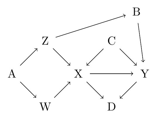
Figure 1: Ground truth causal graph of the synthetic data. The variables $Z,W,X,Y$ form a $Y$-structure after controlling for $A,B,C$

We will pretend we only will have access to the resulting sample, and not to the generative equations nor the causal graph. Our goal will be to verify that the context $S=\{A,B,C\}$ is a proper control set to measure the causal effect of the exposure $X$ and the outcome $Y$.

Y-tests can help us do this. To verify the proposed control set we aim to identify an instrument in the data - a cause of the exposure that is not statistically related to the outcome except through the exposure. In order to verify that an instrument fulfills this condition, we need an auxiliary instrument that is independent of the first instrument in the context $S$, but becomes dependent after controlling for the exposure.

In our example, we can see in the causal graph that the variables $Z$ and $W$ verify these instrumentality conditions with respect to the exposure $X$ and the outcome $Y$ in the context $S=\{A,B,C\}$.

In practice, we do not have access to the causal graph. Instead we need to check these conditions statistically. Concretely, we need to check that (in context $S$) (1) conditioning on $X$ activates the correlation between $Z,W$ and (2) conditioning on $X$ deactivates the correlation between $Z,Y$.

This is not an operational recipe yet. In order to confirm that these conditions are fulfilled, we need to perform the following subchecks: (1a) $Z$ and $W$ are independent in $S$, (1b) $Z$ and $W$ are dependent in $S\cup\{X\}$, (2a) $Z$ and $Y$ are conditionally dependent after controlling for $S$, and that (2b) $Z$ and $Y$ are conditionally independent after controlling for $S\cup\{X\}$.

These four checks guarantee that the context $S$ blocks all non causal paths between $X$ and $Y$. Hence we can (3) measure the causal effect of $X$ on $Y$, by measuring their correlation in context $S$.

You can see the results of applying this analysis to our example in table 1.

Table 1: Five steps of the Y test applied to our example.

step	regression	r	sd	p
1a	Z ~ W S	-0.0148	0.0734	0.8411
1b	Z ~ W | X, S	-0.3708	0.0736	0.0000
2a	Y ~ Z | S	0.8031	0.2316	0.0008
2b	Y ~ Z | X,S	-0.0707	0.1635	0.6664
3	Y ~ X | S	1.0460	0.0657	0.0000

The two key observations are that (1) a correlation between the instruments appears after controlling for the exposure and (2) the correlation between one of the instruments and the outcome disappears after controlling for the exposure.

These observations constitute a positive result of the Y-test, and indicate that the context $S$ does indeed block all non causal paths from $X$ to $Y$.

Speaking inexactly, observation (1) ensures that there is no reverse path from $X$ to $Z$, and the observation (2) ensures that at most one of $Z$ and $Y$ are causes of $X$.

Furthermore, this proves that $S$ is a proper control set for measuring the causal effect of $X$ on $Y$. Therefore, the correlation coefficient on the last regression is an unbiased estimate of the causal effect of $X$ on $Y$.

We provide a formal proof of the soundness of the Y-test in appendix A.

2. A practical version of the y-test

While sound in theory, the y-test is rarely practical because of two requirements:

1. Identifying a context $S$ that blocks all non-causal paths between $X$ and $Y$

2. Identifying two conditionally independent instruments $Z,W$

The first requirement forces us to treat y-tests as a test for omitted variable bias. If we already know there is an unobserved confounder we cannot block, then the test will invariably fail. Therefore, by contraposition, if the test returns positive, then we will have effectively ruled out such confounders.

The second requirement is often hard to meet in practice. Finding a valid instrument is hard enough - finding two that we can render conditionally independent is practically impossible.

Therefore, if we hope to apply the y-test in a practical context, we need to relax this requirement.

The reason why we need the instruments $Z$ and $W$ to be conditionally independent is so we can verify that $X$ activates the correlation between $Z$ and $W$, and thus rule out the possibility of a causal path from $X$ to $Z$.

Sometimes we can get away with this assumption when we have temporal information about the variables - in principle, if $Z$ happened before $X$ then we can rule out reverse causation appealing to the temporal logic of causation. But when our data does not have such a clear temporal ordering we need an alternative.

Hence we need to find an intermediate test that allows us to distinguish the cases where $Z$ is an effect of $X$ or there is a common cause for both from the cases where $Z$ is a cause of $X$.

In order to find such a test, we study the 8 causal graphs that exhaust all possible relations between $Z,W,X$ in a context $S$, assuming that 1) the graph between $Z,X,W$ is complete, 2) $Z$ and $W$ are dependent via a hidden, uncontrollable common cause. See figure 2 for a graphical representation of the selected graphs.

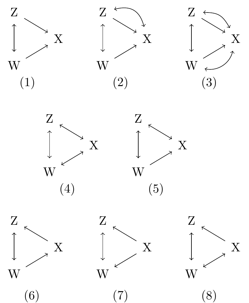
Figure 2: Causal graphs we are studying. Single arrows denote a direct linear causal relation. Double arrows denote a hidden common cause inducing a spurious correlation between the variables.

These 8 graphs include three graphs where there is a path from $X$ to either $Z$ or $W$ (graphs (6), (7), (8)). This is the situation we need to rule out for the Y-test to come out positive.

In order to rule out this possible path from $X$ to $Z$, we will study random representatives of each of the 8 graphs we are interested in. To do this, we define generative functions, which randomly sample coefficients for the edges in the graph and then sample iid observations from the resulting causal system.

See below an example of such a generative function for the graph where both $Z$ and $W$ are causes of $X$ (graph (1)). The definition of the generative functions corresponding to graphs (2-8) are shown in appendix B.

sigma <- 5 # Std of the gaussian noise

# Function to sample path coefficients

sample_coefficients <- function(n){

  abs_value <- sample(c(-1,1), n,

                      replace=TRUE)

  sign <- sample(1:2, n, replace=TRUE)

  coef <- abs_value*sign

  return(coef)

}

# Each graph is described by a generative

# function that randomly samples its path

# coefficients and then returns a sample

# of the constructed graph

"(1)" = function(n){

  alpha <- sample_coefficients(4)

  A <- sigma*rnorm(n)

  Z <- alpha[1]*A + rnorm(n)

  W <- alpha[2]*A + rnorm(n)

  X <- alpha[3]*Z + alpha[4]*W + rnorm(n)

  data <- data.frame(Z,X,W)

  return(data)

}

Now that we have a way of constructing and sampling random representatives for each of the possible graphs, we can study different properties of each of them. The goal will be to find a property that is true only of graphs where there are no paths from $X$ to $Y$.

We focus on (1) whether the correlation between $Z$ and $W$ weakens or becomes stronger after controlling for $X$ (in terms of its p-value), and (2) whether the sign of the correlation between $Z$ and $W$ remains the same after controlling for $X$.

We look at 1000 representatives of each of the 8 graphs, sample 50 independent observations from each representative and check whether either of the properties (1,2) hold for each sample. The results of the experiment are summarized in table 2.

Table 2: Computational study. For each graph we sample a random structural representative, and take 50 samples from the representative. Then we check whether in each sample there is a p value strengthening, a reversal of the correlation point estimate or either of the two former.

Graph	Strengthening	Reversal	Strengthening or reversal
(1)	230	526	756
(2)	848	449	962
(3)	651	351	797
(4)	549	64	594
(5)	548	334	779
(6)	111	498	518
(7)	532	245	561
(8)	552	323	632

Let’s interpret the results of this exploration.

There are three hypotheses of interest to consider: A) both Z and W are causes of X (graphs G1,G2,G3) B) X is a cause of either Z or W (graphs G6,G7,G8) C) $X$ is not a cause of neither $Z$ nor $W$ but either $X$ is not an effect of $Z$ or $W$ is not a cause of $X$ (graphs G4,G5)

We recall that the hypothesis we wish to rule out is B. If we could rule it out, then we could apply the second part of the Y-test to conclude that our control set $S$ is proper.

We then observe that either there is a decreasing p-value or a sign reversal (E) or the opposite (~E).

We want to figure out how either result changes our beliefs about the likelihood of the different hypotheses. In order to do so we need to follow Bayes rule and look at the likelihood of the evidence given the different hypothesis: $P(E|A):P(E|B):P(E|C)$ and $P(~{}E|A):P(~{}E|B):P(~{}E|C)$.

Each hypothesis encompasses several possible graph structures, and hence we have to assign them a relative prior probability beforehand. For example, we will assign them equal probabilities, except for those graphs which have a symmetric counterpart after exchanging the role of $Z$ and $W$ (graphs G2, G5, G6 and G8), to which we will assign twice the prior probability.

Once we have done that, we can resort to our computational study for a crude estimation of the likelihoods. For example:

$$P(E|A)=P(E|G_{1})P(G_{1}|A)+P(E|G_{2})P(G_{2}|A)+P(E|G_{3})P(G_{3}|A)\approx\frac{756}{1000}`\frac{1}{4}+\frac{962}{1000}\frac{2}{4}+\frac{797}{1000}\frac{1}{4}=0.86925$$

Applying this reasoning to the rest of the likelihoods we finally conclude that $P(E|A):P(E|B):P(E|C)\approx 0.189:0.2072:0.198$ and that $P(\neg E|A):P(\neg E|B):P(\neg E|C)\approx 0.811:0.7928:0.802$.

Hence a positive observation provides twice as much evidence for hypothesis A than for hypothesis B, whereas a negative observation provides 10 times more evidence in favor of hypothesis A relative to hypothesis B.

This means that we can use the indicator $E$ as a falsification test for $A$. When the indicator is positive it does not provide a strong signal, so false positives are likely, but a negative is a strong indication that $Z$ is a cause of $X$.

This is to be expected - in the graphs corresponding to hypothesis A, controlling for the $X$ opens up another path through which information can flow, which for typical coefficient values and a representative sample results in either a stronger correlation or an outright reversal of the correlation.

Unfortunately the signal is not very useful for distinguishing hypothesis C from hypothesis B. The likelihood ratio between these given E is about 1.3 in favor of C, and given $\neg E$ it is about 2 in favor of B - not a very strong distinction. But we can live with this downside: most often, the proposed instruments are both hypothesized to be causes of the exposure (hypothesis A), and hence hypothesis $A$ is the one we are more interested in falsifying.

This concludes our analysis and shapes our new test. Once we have attempted to falsify that the instrument $Z$ is a cause of $X$ in context $S$ using this signal, we can proceed to check that the exposure $X$ deactivates the correlation between the instrument $Z$ and the outcome $Y$ in context $S$ to conclude that $S$ is a proper control set, and measure the unbiased effect of $X$ on $Y$ by controlling for $S$.

In the next section we will show how to apply this modified y-test with real econometric data.

3. Effect of price on cigarette demand

As a practical illustration, we consider the problem of modeling the effect of cigarette price on demand at the US state level. We work with the same data as is used in Stock and Watson (2011) to illustrate the application of a generalized two-stage regression model.

This dataset is a good fit for our purposes since (1) it purportedly includes two instruments, making the Y-test applicable, and (2) there are strong theoretical reasons to expect that price causally influences demand and the two instruments shown (two types of taxes) are causes of the price.

We first load the dataset and replicate the original two stage regression.

We are working with five variables, aggregated at state level: the outcome is the number of cigarette packs bought, the exposure is the price of the cigarettes, the instruments are state-specific general tax sale and the cigarette tax sale, and the context we control for includes the income per capita. We work with data from 1995.

In the original analysis an assumption is made that the outcome is causally downstream from the exposure and that, after controlling for income, the taxes are proper instruments for the relation we intend to study. An estimation of the causal effect of the price on demand is made through a two stage linear regression. We replicate their results in table X.

Table 3:

term	estimate	std.error	statistic	p.value
(Intercept)	9.8949555	0.9592169	10.315660	0.0000000
log(rprice)	-1.2774241	0.2496100	-5.117680	0.0000062
log(rincome)	0.2804048	0.2538897	1.104436	0.2752748

Hence, if the causal assumptions made by the authors hold, we conclude that price and demand are negatively correlated, as predicted by standard microeconomic theory.

The interesting part that we can add on is that we can attempt to falsify these causal assumptions using the modified y-test from the last section.

Again, this will require us to study the contextual relationship between the instruments before and after controlling for the exposure (steps 1a and 1b respectively), and the contextual relationship between one of the instruments and the outcome before and after controlling for the exposure (steps 2a and 2b respectively). Finally we will report the contextual correlation between exposure and outcome after controlling for our candidate control (step 3) The results are summarized in table @ref(results_cigs).

Table 4: Five steps of the heuristic Y test applied to the data on cigarette sales.

step	regression	r	sd	p
1a	salestax ~ cigtax | log(rincome)	0.1721	0.0388	0.0001
1b	salestax ~ cigtax | log(rprice) + log(rincome)	-0.2407	0.0669	0.0008
2a	log(packs) ~ cigtax | log(rincome)S	-0.0148	0.0034	0.0001
2b	log(packs) ~ cigtax | log(rprice) + log(rincome)	0.0075	0.0078	0.3415
3	log(packs) ~ log(rprice) | log(rincome)	-1.4065	0.2609	0.0000

We observe that the cigarette tax per state, the price of cigarettes per state and the demand for cigarettes exhibit a chain-like behaviour - the tax and demand are conditionally dependent (2a), but they become independent after controlling for the price (2b).

We, however, find that the instruments are positively correlated before conditioning for the exposure (1a). Hence the traditional y-test would not be able to detect the causal relationship between price and packs bought.

But we observe (1) that the instruments exhibit a correlation reversal after controlling for the exposure - which increases our confidence that the exposure is an effect of both instruments, as we explain in section 2.

One concern with this analysis is that this reversal could be driven by outliers. As a simple test to rule out this possibility, we can plot the data for the two instruments, using color to represent states where the cigarette prices are similar.

While there are some outlier states where the sales tax is below 2% and another outlier state where the cigarette-specific tax is over 60%, at first glance the reversal seems to not be spurious.

This data provides moderate evidence that the two instruments, the exposure and the outcome form a Y-structure, and hence that the packs bought are causally downstream from the prices and that we are not missing any important confounders.

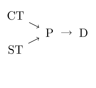
Figure 3: Highest likelihood subgraph according to the y-test, relating the cigarette tax ($CT$), the general sales tax $ST$, the price per pack of cigarettes ($P$) and the demand for cigarettes ($D$) after controlling for income

Indeed, we see that the point estimate after controlling for income falls within the 70% confidence estimate of the two-stage instrument regression, which indicates that all important confounders are controlled for.

4. Effect of firm loans on sales

We saw that our proposed heuristic method for verifying the completeness of the control set was effective in the context of cigarette prices and demand. In this section, we apply our test to another use case to further explore how applicable the proposed method is in practice.

Concretely, we replicate and examine the results of one of the instrumental analyses performed in ‘Do firms want to borrow more?’ (Banerjee and Duflo 2014).

The study is looking at whether firms in India are credit constrained. It does so by studying the causal effect of the change in log working capital limit granted, previous to current year, (ldgl) and their subsequent change of log gross sales (dlgsf).

Four variables are used as controls: the dummy post is equal to 1 in years 1999 and 2000, zero otherwise. The dummy post2 is equal to 1 in years 2001–2002, zero otherwise. The dummy big is equal to 1 for firms with a large investment in plant and machinery, zero otherwise. The dummy big2 is equal to 1 for firms with a very large investment in plant and machinery.

The interactions post*med, post2*big2 and post*big2 are used as instruments. med is a dummy indicating that the firm’s investment in plant and machinery is medium.

The authors decided to filter some outliers, restricting their analysis to firms where the response variable ldgl is contained between -1 and 1.

We replicate Banerjee and Duflo (2014) results in table X. The analysis is a straightforward two-stage instrumental variable analysis with multiple instruments, studying the causal relationship between the variables ldgl, the loan, and dlgsf, gross sales.

Table 5:

term	estimate	std.error	statistic	p.value
(Intercept)	-0.0434255	0.1121425	-0.3872355	0.6986960
ldgl	1.1907750	1.0479873	1.1362495	0.2562292
post	0.0389093	0.0472279	0.8238621	0.4102900
post2	-0.0060974	0.0557906	-0.1092908	0.9130022
big	0.0223917	0.0534700	0.4187709	0.6755081
big2	0.0354311	0.0710304	0.4988158	0.6180611

Our estimate of the effect of ldgl on dlgsf is 1.190775 (coeftest_result[‘ldgl’,‘Std. Error’]). This result does not exactly match the paper results, but falls within a standard deviation of their estimate.

Regardless, we want to check the validity of the proposed instruments. For this we apply the procedure developed in this article, focusing on two of the instruments, namely the post*med interaction and the post2*big2 interaction. The summary of the results can be found in table @ref(tab:causality_test_dufflo_results).

Table 6: Five steps of the heuristic Y test applied to the data on firm credit loans.

step	regression	r	sd	p
1a	postmed ~ post2big2 | post + post2 + big + big2	-0.0362888	0.0122679	0.0031727
1b	postmed ~ post2big2 | ldgl + post + post2 + big + big2	-0.0345640	0.0124107	0.0054588
2a	dlgsf ~ post2*big2 | post + post2 + big + big2	-0.1336647	0.1168405	0.2530057
2b	dlgsf ~ post2*big2 | ldgl + post + post2 + big + big2	-0.1118817	0.1186749	0.3461204
3	dlgsf ~ ldgl | post + post2 + big + big2	0.2004837	0.0729202	0.0061205

We find that the two of the instruments we focus on (namely post*med and post2*big2) have a strong correlation, r=-0.0362888(0.0122679). p=0.0031727. Furthermore, they remain correlated at a lower level of significance, and exhibit no reversal, after controlling for the exposure, at r=-0.034564(0.0124107). p=0.0054588. This suggests that the instruments are not both causal ancestors of the exposure, since we would not expect that to happen in typical v-structures.

Furthermore, the correlation between the outcome dlgsf and the instrument ldgl is barely affected by conditioning on the exposure. This suggests that either the main relationship between the instrument ldgl and the outcome dlgsf is not mediated through the exposure or there is an unobserved confounder.

The above observations seem to weaken the case for (Banerjee and Duflo 2014) analysis. Particularly, the absence of a significant instrument correlation after controlling for the exposure seems to invalidate the implicit causal assumptions of the IV analysis conducted.

However we can build a toy model following the author’s assumptions that replicates the phenomena observed in the data quite faithfully. This is evidence that our heuristic is misleading in this case.

# Example of a data generation process

# where there heuristic Y-test fails

n <- 100

z1 <- rnorm(n) < 0.

z2 <- rnorm(n) < 1.

z3 <- rnorm(n) < -1.

i1 <- z1*z2

i2 <- z2*z3

e <- i1 + i2 + z1 + z2 + z3 + rnorm(n)

o <- e + z1 + z2 + z3 + rnorm(n)

## [1] "i1 ~  i2 | s1 + s2 + s3 = 0.05 [0.27], p=0.8445588759"

## [1] "i1 ~  i2 | e + s1 + s2 + s3 = 0.06 [0.27], p=0.8265246505"

The result in this simulation is that, as with the real dataset, the correlation of the instrument does not vary much after controlling for the exposure ; executing the piece of code above a few times will convince the reader that this result is not atypical.

Hence we conclude that our heuristic test is not guaranteed to be informative outside of the strict Gauss linear systems with approximately uniform distribution of coefficients where we developed our heuristic in section 2.

Characterizing scenarios where the heuristic is unreliable remains an open question; for example in this dataset it may be because of the use of binary interactions as instruments or because the contextual independences present in the data.

5. Conclusion and open questions

In this article, we have explained how to use the Y-test to identify causal relationships using two conditionally independent instruments.

Under the reasoning that this test is too restrictive in practice, we have done a computational study of causal graphs that helped us identify a weaker requirement than conditionally independent instruments. We show that if the strength of the correlation between the instruments diminishes after controlling for the exposure but there is no reversal, that is a strong indication that at least one of the instruments is not a cause of the exposure.

Finally, we have shown how to apply this modified y-test in the context of a price-demand elasticity problem.

The practicality of this test is yet in question. For example, in section 4 we have shown an example of a dataset where our proposed heuristic is misleading. Understanding better where it is appropriate to rely on this statistic is an important next step.

The high rate of false positives is also concerning, but it is to be expected in such low-data scenarios, so we could argue that, in that respect, the proposed test is not different from other econometric tools. Of course, there are tools which have better asymptotic properties that we cannot guarantee for our test - whether the test will be misleading depends primarily on the underlying causal structure, not the amount of data collected.

While the test we propose is still quite restrictive on its conditions of application (as it requires the identification of two presumed instruments), it successfully relaxes the stringent condition of instrument independence required by the Y-test. We hope this heuristic will be a useful concept for the econometrician’s toolbox - primarily as a test to falsify a proposed control set.

5.1 Future work

In principle, the Y-test could be extended to deal with possibly non-linear, non-gaussian processes by using an appropriate conditional independence test.

Another question we haven’t considered is whether this reasoning can be extended to contexts with possibly cyclical causal dependencies, and context where there is selection bias.

We also might be interested in considering the possibility of multiple Y-tests supporting contradictory results. Naively, we could take them as independent evidence that cancels out - but this is unsatisfactory, as we would expect that different tests provide different strength of evidence.

Lastly, while the Y-test is sound, it is not complete - there are causal relationships that can be determined from conditional independence tests that cannot be detected applying the Y-test. Hence we could use more general principles of causal discovery such as the ones exposed in Zhang (2008) or Claassen and Heskes (2011) to build more general tests.

References

Banerjee, Abhijit V., and Esther Duflo. 2014. “Do Firms Want to Borrow More? Testing Credit Constraints Using a Directed Lending Program.” The Review of Economic Studies 81 (2): 572–607. https://doi.org/10.1093/restud/rdt046.

Claassen, Tom, and Tom Heskes. 2011. “A Structure Independent Algorithm for Causal Discovery.” In In ESANN’11, 309–14.

Glymour, Clark, Kun Zhang, and Peter Spirtes. 2019. “Review of Causal Discovery Methods Based on Graphical Models.” Frontiers in Genetics 10. https://doi.org/10.3389/fgene.2019.00524.

Mani, Subramani, Peter L. Spirtes, and Gregory F. Cooper. 2012. “A Theoretical Study of Y Structures for Causal Discovery.” arXiv:1206.6853 [Cs, Stat], June. http://arxiv.org/abs/1206.6853.

Messerli, Franz H. 2012. “Chocolate Consumption, Cognitive Function, and Nobel Laureates.” New England Journal of Medicine 367 (16): 1562–4. https://doi.org/10.1056/NEJMon1211064.

Reiersöl, Olav. 1945. “Confluence Analysis by Means of Instrumental Sets of Variables.” /paper/Confluence-analysis-by-means-of-instrumental-sets-Reiers%C3%B6l/e24fab07b33f9521febf11ccdbea0d5bdb38f927.

Sargan, J. D. 1958. “The Estimation of Economic Relationships Using Instrumental Variables.” Econometrica 26 (3): 393–415. https://doi.org/10.2307/1907619.

Stock, James H., and Mark Watson. 2011. Introduction to Econometrics: International Edition. 3rd edition. Boston, Mass.: Pearson Education.

Zhang, Jiji. 2008. “On the Completeness of Orientation Rules for Causal Discovery in the Presence of Latent Confounders and Selection Bias.” Artificial Intelligence 172 (16): 1873–96. https://doi.org/10.1016/j.artint.2008.08.001.

A. Proof of the soundness of the Y-test

Before we can state the theorem we need some preliminary definitions.

Definition 1 - Causal structural model

A structural causal model consists of a set of variables $X=\{X_{1},...,X_{n}\}$, noise terms $U_{1},...,U_{n}$ and a set of functional constraints $X_{i}=f_{i}(pa(X_{i}),U_{i})$, where $pa(X_{i})\subset X$ is a subset of the variables called the parents or direct causes of $X_{i}$.

Associated to a causal structural model we have a causal graph, which is a directed graph $G=<X,E>$ whose nodes are the variables $X$ and there is an edge from $X_{i}$ to $X_{j}$ iff $X_{i}\in pa(X_{j})$.

We say that a structural causal model is acyclic if the parenthood relation induces an acyclic causal graph.

Definition 2 - d-separation and faithfulness

We say that a trail $A_{1}-A_{2}-...-A_{n}$ in a directed acyclic graph $G=<X,E>$ is blocked in a context $S$ iff either (1) it contains a chain $A_{i-1}\rightarrow A_{i}\rightarrow A_{i+1}$ such that $A_{i}\in S$, (2) it contains a fork $A_{i-1}\leftarrow A_{i}\rightarrow A_{i+1}$ such that $A_{i}\in S$ or (3) it contains a collider $A_{i-1}\rightarrow A_{i}\leftarrow A_{i+1}$ such that neither $A_{i}$ nor any of its descendants are in $S$.

We say that two variables $A,B$ in a directed acyclic graph are d-separated by a context $S\subset X$ iff every trail between $A,B$ is blocked by $S$.

We say that two variables $X_{i},X_{j}$ in a structural causal model are conditionally independent given a context $S\subset X$ iff $X_{i}$ and $X_{j}$ are conditionally independent for any possible assignment for the context $S=s$. We write this as $X_{i}\perp X_{j}|S$.

We say that an acyclic structural causal model is faithful when there is a one-to-one correspondence between d-separation in the causal graph and conditional independence. That is, when $X_{i}\perp X_{j}|S$ iff $X_{i}$ and $X_{j}$ are d-separated by $S$ in its associated causal graph.

Theorem 1 - Soundness of the y-test

Let’s assume that we have four variables $A,B,Z,W$ and a context $S$ in an acyclical and faithful causal structural model such that: 1. $Z\perp W|S$ and $Z\perp W|S\cup\{A\}$ 2. $Z\not\perp B|S$ and $Z\perp B|\cup\{A\}$ 3. $A\not\perp B|S$

Then we can conclude that $A$ is a cause of $B$, ie there exists a fully directed path $A\to B$ in the causal diagram associated to the system.

Furthermore, $S$ is a proper controlling set for $A\to B$ - it blocks all and only the non causal paths from $A$ to $B$.

Proof sketch -

Our goal is to show that there exists a directed path $A\to B$ in the causal graph.

Let $Z-W$ be a trail between $Z$ and $W$ that becomes active in context $S\cup\{A\}$. Because of d-separation properties, in this trail $A$ is either a collider or the children of a collider. In either case, it is true that there exists an active trail $Z\to_{S}A$ such that the last edge points towards $A$.

Now, let $A-_{S}B$ be any active trail between $A,B$ in context $S$ (we know that such a trail must exist since we assumed that $A\not\perp B$ in context $S$).

Consider the concatenated trail $Z\to_{S}A-_{S}B$, which we know is active in $S$. Because of our assumption that $Z\not\perp B|S$ and $Z\perp B|\cup\{A\}$, any active trail between $Z,A,B$ in $S$ becomes blocked in context $S\cup\{A\}$. Hence, we know that $A$ is not a collider in this particular trail. Since we already know that there is an incident edge $Z\to_{S}A$ in the trail, we must conclude that the first edge in the trail $A-_{S}B$ points away from $A$.

Hence, either $A-_{S}B$ is a directed path from $A\to B$ or there exists a collider in the path that is activated by $S$.

But suppose that there existed a collider in the trail $A-_{S}B$. Pick whichever collider is closer to $A$. For the trail to be active, the collider must be active, so either the collider itself is in $S$ or a direct descendant of the collider is in $S$. Either way, since the closest collider to $A$ is a direct descendant of $A$, then we have that a direct descendant of $A$ is in $S$.

But that cannot be, since $A$ was either a deactivated collider or the direct descendant of a deactivated collider in the trail $Z-_{S}W$. Hence we conclude that every active trail $A-_{S}B$ is a fully directed path from $A$ to $B$. In particular, there exists some fully directed path $A\to B$, hence $A$ is a cause of $B$.

Additionally, we can show that no fully directed trail from $A\to B$ is blocked by $S$. Indeed, if it was otherwise, when there would be a descendant $C$ of $A$ such that $C\in S$. But then $C$ would be a common descendant of $Z$ and $W$ in $S$, and we would have that $Z\not\perp W|S$, against our premise. Hence $S$ is a proper control set for $A\to B$ - it blocks all and only the non causal trails from $A$ to $B$.

$\square$

B. Definition of the generative functions to sample graphs

The code below is used to generate random graphs from which to sample in section 2.

# Function to randomly sample path coefficients

sample_coefficients <- function(n){

  abs_value <- sample(c(-1,1), n, replace=TRUE)

  sign <- sample(1:2, n, replace=TRUE)

  coef <- abs_value*sign

  return(coef)

}

# List of representative causal graphs

# Each graph is described by a generative

# function that randomly samples its path

# coefficients and then returns a sample

# of the constructed graph

graphs <- list(

    "(1)" = function(n){

    alpha <- sample_coefficients(4)

    A <- sigma*rnorm(n)

    Z <- alpha[1]*A + rnorm(n)

    W <- alpha[2]*A + rnorm(n)

    X <- alpha[3]*Z + alpha[4]*W + rnorm(n)

    data <- data.frame(Z,X,W)

    return(data)

  },

  "(2)" = function(n){

    alpha <- sample_coefficients(6)

    A <- rnorm(n)

    B <- rnorm(n)

    Z <- alpha[1]*A + alpha[2]*B + rnorm(n)

    W <- alpha[3]*A + rnorm(n)

    X <- alpha[4]*B + alpha[5]*W + alpha[6]*Z

         + rnorm(n)

    data <- data.frame(Z,X,W)

    return(data)

  },

  "(3)" = function(n){

    alpha <- sample_coefficients(8)

    A <- rnorm(n)

    B <- rnorm(n)

    C <- rnorm(n)

    Z <- alpha[1]*A + alpha[2]*B + rnorm(n)

    W <- alpha[3]*A + alpha[4]*C + rnorm(n)

    X <- alpha[5]*B + alpha[6]*C + alpha[7]*Z

         + alpha[8]*W + rnorm(n)

    data <- data.frame(Z,X,W)

    return(data)

  },

  "(4)" = function(n){

    alpha <- sample_coefficients(6)

    A <- rnorm(n)

    B <- rnorm(n)

    C <- rnorm(n)

    Z <- alpha[1]*A + alpha[2]*B + rnorm(n)

    W <- alpha[3]*A + alpha[4]*C + rnorm(n)

    X <- alpha[5]*B + alpha[6]*C + rnorm(n)

    data <- data.frame(Z,X,W)

    return(data)

  },

  "(5)" = function(n){

    alpha <- sample_coefficients(5)

    A <- rnorm(n)

    B <- rnorm(n)

    Z <- alpha[1]*A + alpha[2]*B + rnorm(n)

    W <- alpha[3]*A + rnorm(n)

    X <- alpha[4]*B + alpha[5]*W + rnorm(n)

    data <- data.frame(Z,X,W)

    return(data)

  },

  "(6)" = function(n){

    alpha <- sample_coefficients(4)

    A <- rnorm(n)

    W <- alpha[1]*A + rnorm(n)

    X <- alpha[2]*W + rnorm(n)

    Z <- alpha[3]*A + alpha[4]*X + rnorm(n)

    data <- data.frame(Z,X,W)

    return(data)

  },

  "(7)" = function(n){

    alpha <- sample_coefficients(4)

    A <- rnorm(n)

    X <- rnorm(n)

    W <- alpha[1]*A + alpha[2]*X + rnorm(n)

    Z <- alpha[3]*A + alpha[4]*X + rnorm(n)

    data <- data.frame(Z,X,W)

    return(data)

  },

  "(8)" = function(n){

    alpha <- sample_coefficients(5)

    A <- rnorm(n)

    B <- rnorm(n)

    W <- alpha[1]*A + alpha[2]*B + rnorm(n)

    X <- alpha[3]*B + rnorm(n)

    Z <- alpha[4]*A + alpha[5]*X + rnorm(n)

    data <- data.frame(Z,X,W)

    return(data)

  }

)

C. List of variables used in the analysis

Variables used for the analysis in section 3:

Table 7:

Variable	Meaning
salestax	Percentage amount of general tax over goods in a state
cigtax	Percentage amount of tax over cigarettes in a state
rprice	Price of a cigarette pack, adjusted for inflation
rincome	Average income per capita, adjusted for inflation

Variables used for the analisis in section 4:

Table 8:

Variable	Meaning
dlgsf	Change in log working capital limit granted, previous to current year
ldgl	Change of log gross sales, previous to current year
post	Indicator of whether the year is 1999-2000
post2	Indicator of whether the year is 2001-2002
big	Indicator of whether investment in plant and machinery is larger than Rs. 6.5 million
big2	Indicator of whether investment in plant and machinery is larger than Rs. 10 million
med	Indicator of whether investment in plant and machinery is between than Rs. 6.5 million and Rs. 10 million