Complexity of Source-Sink Monotone 2-Parameter Min Cut

Abstract

There are many applications of max flow with capacities that depend on one or more parameters. Many of these applications fall into the “Source-Sink Monotone” framework, a special case of Topkis’s monotonic optimization framework, which implies that the parametric min cuts are nested. When there is a single parameter, this property implies that the number of distinct min cuts is linear in the number of nodes, which is quite useful for constructing algorithms to identify all possible min cuts.

When there are multiple Source-Sink Monotone parameters, and vectors of parameters are ordered in the usual vector sense, the resulting min cuts are still nested. However, the number of distinct min cuts was an open question. We show that even with only two parameters, the number of distinct min cuts can be exponential in the number of nodes.

1 Introduction

There are many problems that can be formulated as Max Flow/Min Cut networks such that the capacities of the arcs depend on one or more parameters. This problem is known as parametric Max Flow/Min Cut, see e.g.[7] for a recent survey. In such applications, we may be interested in identifying the parameters which maximize the flow value, or which lead to the zero of an auxiliary function.

Typically, the capacities of the arcs are affine functions of the parameters (but see [8] for some exceptions). In this setting, it is easy to see that the region of the parameter space where a specific min $s$–$t$ cut (hereafter min cut) is optimal, which we call a cell, is a polyhedron. The interiors of these cells are disjoint and so induce a partition of the parameter space. If the number of cells for some class of instances is “small” (polynomial in the size of the network), then an algorithm could try to construct all of the cells and efficiently solve the parametric problems in this class. However, if the number of cells can be exponential in the size of the networks, this algorithmic strategy is ruled out. This makes it interesting to study the complexity of classes of parametric networks, namely the worst-case number of cells in the class. In general parametric networks, Carstensen [3] showed that the number of cells can be exponential in the number of nodes in the network, even with just one parameter.

On the other hand, Gallo, Grigoriadis, and Tarjan [6] (hereafter GGT) showed that a class of parametric networks with many applications has only a linear number of cells. Suppose that there is a single scalar parameter $\lambda$, and that all capacities are affine in $\lambda$. We write an arc with tail $i$ and head $j$ as $i\to j$, and its (upper) capacity as $u_{ij}(\lambda)=a_{ij}\lambda+c_{ij}$ ($\lambda$ is implicitly restricted to a domain where all capacities are non-negative). The nodes of the network are the source $s$, the sink $t$, and the internal nodes $N$ with $n=|N|$. Following [7], we say that a parametric network is Source-Sink Monotone (SSM) if

$$u_{sj}(\lambda) \lambda s$$ is non-decreasing in for all arcs exiting

(i.e., $$a_{sj}\geq 0$$);

$$u_{it}(\lambda) \lambda t$$ is non-increasing in for all arcs entering

(i.e., $$a_{it}\leq 0$$);

$$u_{ij}(\lambda) \lambda$$ is constant in for all other arcs

(i.e., for all $$i\neq s j\neq t a_{ij}=0$$ and , ). (1)

GGT showed that SSM networks have at most $n$ cells, and so at most $n$ distinct min cuts. This is quite convenient for construction of algorithms, and indeed another major contribution of GGT is an algorithm that computes all of the min cuts in the same asymptotic time as a single max flow computation. These results were generalized to larger classes of networks with a single parameter in [7], and to parametric min-cost flow networks in [10].

There are applications where multiple parameters arise naturally. One broad class is problems with multiple objectives (see [5] for a survey), where it is natural to model $k$ objectives by introducing $k-1$ parameters to obtain another model with a single objective equal to a linear combination of the original $k$ objectives. Other examples include a scheduling application of Chen [4] and a budgeted network interdiction problem [13]. Thus it is interesting to extend the GGT-type results to multiple parameters.

Notice that the definition of SSM extends naturally to multiple parameters if we replace “$\lambda$” with “$\lambda_{1},\dots,\lambda_{k}$”. In fact, the GGT result which proves that single-parameter SSM networks have at most $n$ cells is a special case of a more general result on monotone parametric optimization on lattices by Topkis [18, 19]. When specialized to SSM parametric networks with parameters $\lambda_{1}$, $\lambda_{2}$, …, $\lambda_{k}$, Topkis’s framework looks like this: Let $S(\lambda_{1},\dots,\lambda_{k})$ denote a min cut at $(\lambda_{1},\dots,\lambda_{k})$. If $(\lambda_{1},\dots,\lambda_{k})\leq(\lambda^{\prime}_{1},\dots,\lambda^{\prime}_{k})$ (in the usual partial order on real vectors), then $S(\lambda_{1},\dots,\lambda_{k})\subseteq S(\lambda^{\prime}_{1},\dots,\lambda^{\prime}_{k})$ and the min cuts are nested. This result gives a quick proof for why single-parameter SSM networks have at most $n$ min cuts: The partial order on real vectors is a total order on $\mathbb{R}^{1}$, which implies that all of the min cuts are nested and there can be at most $n$ min cuts.

When we extend from one SSM parameter to multiple SSM parameters, we still have nested min cuts due to Topkis’s result. However, we only have a partial order on vectors of parameters instead of a total order. What is the complexity of parametric max flow/min cut in this case?

The problem of the complexity of parametric global min cut with $k$ parameters was studied in [2, 9], who showed that there are only $O(n^{k+1})$ cells, which is polynomial for fixed $k$. Given that global min cut and min $s$–$t$ cut seem to be closely related, it is perhaps surprising that our main result is:

Theorem 1.1

There exists instances of SSM max flow/ min cut with two parameters where all $2^{n}$ $s$–$t$ cuts are unique min cuts for some values of the parameters.

We will prove Theorem 1.1 by constructing a family of instances, parameter values, and flows that show that every possible $s$–$t$ cut is a unique min cut at some parameter values. For simplicity we will henceforth denote our two parameters as $\lambda$ and $\mu$, and so the capacity of $i\to j$ is $a_{ij}\lambda+b_{ij}\mu+c_{ij}$. We further specialize the SSM conditions (1) to:

$$u_{sj}(\lambda,\mu) \lambda \mu s$$ is increasing in and for all arcs exiting

(i.e., $$a_{sj},b_{sj}>0$$);

$$u_{ij}(\lambda,\mu) \lambda \mu$$ is constant in and for all other arcs

(i.e., for all $$i\neq s a_{ij}=b_{ij}=0$$, ). (2)

We consider only non-negative values for $\lambda$ and $\mu$. In our construction, the constant term $c_{sj}$ in the parametric arcs with tail $s$ is always zero, and hence the capacities of all arcs $s\to j$ are non-negative for all $\lambda,\mu\geq 0$.

In Section 2, we present the recursive definitions for the networks, parameters values, and flows. In Section 3, we motivate these definitions and give the intuition behind the construction. Section 4 proves a series of lemmas which lead to the proof of Theorem 1.1. Finally, Section 5 discusses some implications of our result.

2 Construction of the Family of Examples

For each $n\geq 1$ we construct a parametric network ${\cal N}^{n}$ satisfying our restricted notion of SSM in (2). Let $N^{n}=\{1,\dots,n\}$ denote the internal nodes of ${\cal N}^{n}$. The set of arcs of ${\cal N}^{n}$ is the union of source arcs $\{s\to j:\;j\in N^{n}\}$, sink arcs $\{j\to t:\;j\in N^{n}\}$, and internal arcs $\{j\to k:\;j,k\in N^{n},j>k\}$. The capacity of arc $s\to j$ is $u^{n}_{sj}(\lambda,\mu)=a^{n}_{sj}\lambda+b^{n}_{sj}\mu$. The constructed values of $a^{n}_{sj}$ and $b^{n}_{sj}$ are positive, which ensures that ${\cal N}^{n}$ is SSM. The capacity of a non-parametric arc $j\to k$ is $u^{n}_{jk}$ for $j\neq s$.

For $S\subset N^{n}$ such that $i\notin S$, we denote $S\cup\{i\}$ by $S+i$. Any $S\subseteq N^{n}$ induces the $s$–$t$ cut $S+s$, but for simplicity we refer to $S$ as the cut. For each $S\subseteq N^{n}$, we construct a point $(\lambda^{n,S},\mu^{n,S})\in(0,1)\times(0,1)$ and a corresponding flow $x^{n,S}$ such that $x^{n,S}$ is a feasible max flow in ${\cal N}^{n}$ with unique min cut $S$ at $(\lambda^{n,S},\mu^{n,S})$. To reduce clutter, let $u_{sj}^{n,S}$ denote the capacity of $s\to j$ at $(\lambda^{n,S},\mu^{n,S})$:

$$u_{sj}^{n,S}=u^{n}_{sj}(\lambda^{n,S},\mu^{n,S})=a^{n}_{sj}\lambda^{n,S}+b^{n}_{sj}\mu^{n,S}.$$

The capacities of the other arcs are constant.

Our construction is recursive so that ${\cal N}^{n}$ is based on ${\cal N}^{n-1}$. For $S\subseteq N^{n-1}$, we construct $(\lambda^{n,S},\mu^{n,S})$ and $(\lambda^{n,S+n},\mu^{n,S+n})$ based on $(\lambda^{n-1,S},\mu^{n-1,S})$, and we construct $x^{n,S}$ and $x^{n,S+n}$ based on $x^{n-1,S}$.

For the base case at $n=1$, let $a^{1}_{s1}=b^{1}_{s1}=1$ so that the arc capacities are:

$$u^{1}_{s1}(\lambda,\mu) =\lambda+\mu,\text{ and }u^{1}_{1t}=1.$$

For $S=\emptyset$, set:

$$(\lambda^{1,\emptyset},\mu^{1,\emptyset})=\left(\frac{1}{4},\frac{1}{4}\right),\text{ with }x^{1,\emptyset}_{s1}=\frac{1}{2}=x^{1,\emptyset}_{1t}.$$

Clearly, the flow $x^{1,\emptyset}$ is feasible and $S=\emptyset$ is the unique min cut. For $S=\{1\}$, set:

$$(\lambda^{1,\{1\}},\mu^{1,\{1\}})=\left(\frac{3}{4},\frac{3}{4}\right),\text{ with }x^{1,\{1\}}_{s1}=1=x^{1,\{1\}}_{1t}.$$

Clearly, the flow $x^{1,\{1\}}$ is feasible and $S=\{1\}$ is the unique min cut. Hence, $S=\emptyset,\{1\}$ are unique min cuts at $(\lambda^{1,\emptyset},\mu^{1,\emptyset})$ and $(\lambda^{1,\{1\}},\mu^{1,\{1\}})$ respectively.

We define two “large” constants for $n\geq 2$ whose definitions will be motivated later:

$$\theta^{n} =3a^{n-1}_{s,n-1},\text{ and}$$ (3)

$$\gamma^{n} =\begin{cases}4&\text{for $n=2$},\\ 4\cdot\sum_{j<n}(\theta^{n}b^{n-1}_{sj}-3a^{n-1}_{sj})&\text{for $n>2$.}\end{cases}$$ (4)

To construct ${\cal N}^{n}$ from ${\cal N}^{n-1}$ for $n>1$, we add node $n$, arcs $s\to n$ and $n\to t$, and arcs $n\to j$ for $j\in N^{n-1}$. The arc capacities for ${\cal N}^{n}$ are as follows:

$$u^{n}_{sj}(\lambda,\mu) =4a^{n-1}_{sj}\lambda+(1+\theta^{n})b^{n-1}_{sj}\mu j\in N^{n-1};$$ for

$$u^{n}_{jt} =u^{n-1}_{jt}+\theta^{n}b^{n-1}_{sj} j\in N^{n-1};$$ for

$$u^{n}_{ij} =u^{n-1}_{ij} i,j\in N^{n-1},i>j;$$ for

$$u^{n}_{nj} =\theta^{n}b^{n-1}_{sj}-3a^{n-1}_{sj} j\in N^{n-1};$$ for

$$u^{n}_{sn}(\lambda,\mu) =\gamma^{n}\lambda+\mu;$$

$$u^{n}_{nt} =\frac{\gamma^{n}}{2}.$$ (5)

By (3), we have $u_{n,n-1}^{n}=0$. Furthermore, we have $a_{sj}^{n}=4a_{sj}^{n-1}$ and $b_{sj}^{n}=(1+\theta^{n})b_{sj}^{n-1}$ for $j\in N^{n-1}$, and $a^{n}_{sn}=\gamma^{n}$ and $b^{n}_{sn}=1$. We will verify that $u^{n}_{nj}\geq 0$ for $j<n$ in Lemma 4.2. See Figures 1 and 2 for ${\cal N}^{2}$ and ${\cal N}^{3}$.

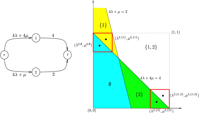
Figure 1: For $n=2$, $\theta^{2}=3$ and $\gamma^{2}=4$, which leads to this parametric network ${\cal N}^{2}$ and its four cells. The two scaled, shifted boxes (outlined in red) are $(0,\frac{1}{4})\times(\frac{3}{4},1)$, and $(\frac{3}{4},1)\times(0,\frac{1}{4})$. The four $(\lambda^{2,S},\mu^{2,S})$ points are marked, and the dotted box $(0,1)\times(0,1)$ contains the two red boxes and the four points. We omit arcs with capacity 0 in the network.

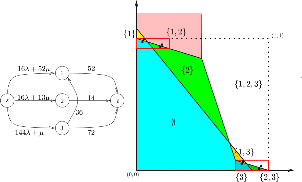
Figure 2: For $n=3$, $\theta^{3}=12$ and $\gamma^{3}=144$, which leads to this parametric network ${\cal N}^{3}$ and its eight cells. The two scaled, shifted boxes (outlined in red) are $(0,\frac{1}{4})\times(\frac{12}{13},1)$, and $(\frac{3}{4},1)\times(0,\frac{1}{13})$, which contain the eight $(\lambda^{3,S},\mu^{3,S})$ points (marked but not labeled). Each red box contains a scaled, shifted copy of the cells for $n=2$. The dotted box $(0,1)\times(0,1)$ contains the two red boxes and the eight points. We omit arcs with capacity 0 in the network.

Let $S\subseteq N^{n-1}$. First, we define the following point at which $S$ will be the unique min cut of the new ${\cal N}^{n}$:

$$(\lambda^{n,S},\mu^{n,S}) =\left(\frac{\lambda^{n-1,S}}{4},\frac{\mu^{n-1,S}+\theta^{n}}{1+\theta^{n}}\right).$$ (6a)

Since each point $(\lambda^{n-1,S},\mu^{n-1,S})\in(0,1)\times(0,1)$, it is easy to see that $(\lambda^{n,S},\mu^{n,S})\in(0,\frac{1}{4})\times(\frac{\theta^{n}}{1+\theta^{n}},1)$. The corresponding flow $x^{n,S}$ is:

$$x^{n,S}_{sj} =x^{n-1,S}_{sj}+\theta^{n}b^{n-1}_{sj} j\in N^{n-1};$$ for

$$x^{n,S}_{jt} =x^{n-1,S}_{jt}+\theta^{n}b^{n-1}_{sj} j\in N^{n-1};$$ for

$$x^{n,S}_{ij} =x^{n-1,S}_{ij} i,j\in N^{n-1},i>j;$$ for

$$x^{n,S}_{nj} =0 j\in N^{n-1};$$ for

$$x^{n,S}_{sn} =x^{n,S}_{nt}=u^{n,S}_{sn}.$$ (6b)

Lemma 4.3 will use this flow $x^{n,S}$ to prove that $S$ is the unique min cut at $(\lambda^{n,S},\mu^{n,S})$.

Next, we define the following point at which $S+n$ will be the unique min cut of ${\cal N}^{n}$:

$$(\lambda^{n,S+n},\mu^{n,S+n}) =\left(\frac{\lambda^{n-1,S}+3}{4},\frac{\mu^{n-1,S}}{1+\theta^{n}}\right).$$ (7a)

Observe that $(\lambda^{n,S+n},\mu^{n,S+n})\in(\frac{3}{4},1)\times(0,\frac{1}{1+\theta^{n}})$. The corresponding flow $x^{n,S+n}$ is:

$$x^{n,S+n}_{sj} =x^{n-1,S}_{sj}+3a^{n-1}_{sj} j\in N^{n-1};$$ for

$$x^{n,S+n}_{jt} =x^{n-1,S}_{jt}+\theta^{n}b^{n-1}_{sj} j\in N^{n-1};$$ for

$$x^{n,S+n}_{ij} =x^{n-1,S}_{ij} i,j\in N^{n-1},i>j;$$ for

$$x^{n,S+n}_{nj} =u^{n}_{nj}=\theta^{n}b^{n-1}_{sj}-3a^{n-1}_{sj} j\in N^{n-1};$$ for

$$x^{n,S+n}_{sn} =\frac{\gamma^{n}}{2}+\sum_{j<n}(\theta^{n}b^{n-1}_{sj}-3a^{n-1}_{sj});$$

$$x^{n,S+n}_{nt} =\frac{\gamma^{n}}{2}.$$ (7b)

Lemma 4.4 will use this flow $x^{n,S+n}$ to prove that $S+n$ is the unique min cut at $(\lambda^{n,S+n},\mu^{n,S+n})$.

3 Intuition behind the Construction

Strong complementary slackness implies that $S$ is the unique min cut at $(\lambda^{n,S},\mu^{n,S})$ if there exists a flow $x^{n,S}$ (which then must be a max flow) satisfying:

$$x^{n,S}_{sj} <u^{n,S}_{sj} j\in S;$$ for

$${\color[rgb]{0.0078125,0.15234375,0.77734375}x^{n,S}_{jt}} {\color[rgb]{0.0078125,0.15234375,0.77734375}{}=u^{n}_{jt}} {\color[rgb]{0.0078125,0.15234375,0.77734375}j\in S};$$ for

$${\color[rgb]{0.0078125,0.15234375,0.77734375}x^{n,S}_{sj}} {\color[rgb]{0.0078125,0.15234375,0.77734375}{}=u^{n,S}_{sj}} {\color[rgb]{0.0078125,0.15234375,0.77734375}j\notin S};$$ for (SCS)

$$x^{n,S}_{jt} <u^{n}_{jt} j\notin S;$$ for

$${\color[rgb]{0.01953125,0.47265625,0.09375}x^{n,S}_{jk}} {\color[rgb]{0.01953125,0.47265625,0.09375}{}=u^{n}_{jk}} {\color[rgb]{0.01953125,0.47265625,0.09375}j\in S,k\notin S,j>k};$$ for

$${\color[rgb]{0.83984375,0,0}x^{n,S}_{jk}} {\color[rgb]{0.83984375,0,0}{}=0} {\color[rgb]{0.83984375,0,0}j\notin S,k\in S,j>k}.$$ for

See Figure 3 for an example and explanation of the colors. Lemmas 4.3 and 4.4 will use (SCS) to prove Theorem 1.1.

Figure 3: ${\cal N}^{n-1}$, denoting $x^{n-1}_{ij}$ by $x^{-}$ and $u^{n-1}_{ij}$ by $u^{-}$. The (SCS) conditions say that if $i\notin S$, then $s\to i$ is saturated (heavy blue), but $i\to t$ is not saturated, and all other $i\to k$ have 0 flow (dotted red); whereas if $j\in S$, then $s\to j$ is not saturated, but $j\to t$ is saturated, and all other $j\to k$ are saturated (heavy green). The dashed source and sink arcs at $k$ indicate that they are saturated depending on whether or not $k$ is in $S$; the (SCS) conditions hold for internal arcs with head $k$ in either case.

First consider the base case of ${\cal N}^{1}$. It is easy to check that our flows $x^{1,\emptyset}$ and $x^{1,\{1\}}$ satisfy (SCS). If we visualize the cuts as cells on the $(\lambda,\mu)$-plane, then we have a box on $(0,1)\times(0,1)$ which contains both points $(\lambda^{1,\emptyset},\mu^{1,\emptyset})=(\frac{1}{4},\frac{1}{4})$ and $(\lambda^{1,\{1\}},\mu^{1,\{1\}})=(\frac{3}{4},\frac{3}{4})$.

For $n>1$, our strategy is to shrink the original box $(0,1)\times(0,1)$ containing all the $(\lambda^{n-1,S},\mu^{n-1,S})$ points into the smaller box $(0,\frac{1}{4})\times(\frac{\theta^{n}}{1+\theta^{n}},1)$. Then for each $S\subseteq N^{n-1}$, the points corresponding to min cuts without node $n$, $(\lambda^{n,S},\mu^{n,S})$, are contained in the box $(0,\frac{1}{4})\times(\frac{\theta^{n}}{1+\theta^{n}},1)$. We also construct a new point for each min cut which contains node $n$, $(\lambda^{n,S+n},\mu^{n,S+n})$, such that the new points are contained in the box $(\frac{3}{4},1)\times(0,\frac{1}{1+\theta^{n}})$. The boxes containing the min cuts with $n$ and without $n$ do not overlap.

When we add node $n$ to ${\cal N}^{n}$, the arc capacities of $s\to n$ and $n\to t$ are $u^{n}_{sn}(\lambda,\mu)=\gamma^{n}\lambda+\mu$ and $u^{n}_{nt}=\frac{\gamma^{n}}{2}$. When $\lambda<\frac{1}{4}$, then $u^{n}_{sn}(\lambda,\mu)$ is “small” relative to $u^{n}_{nt}$ and so any max flow will saturate arc $s\to n$. Hence, node $n$ will not be in any min cut and we can leave the flow on internal arcs $n\to j$ as 0. For each $S\subseteq N^{n-1}$ and $j<n$, (5) and (6a) imply that:

$$u^{n,S}_{sj} =4a^{n-1}_{sj}\left(\frac{\lambda^{n-1,S}}{4}\right)+(1+\theta^{n})b^{n-1}_{sj}\left(\frac{\mu^{n-1,S}+\theta^{n}}{1+\theta^{n}}\right)$$

$$=a^{n-1}_{sj}\lambda^{n-1,S}+b^{n-1}_{sj}\mu^{n-1,S}+\theta^{n}b^{n-1}_{sj}$$

$$=u^{n-1,S}_{sj}+\theta^{n}b^{n-1}_{sj}.$$ (8)

Our construction adds $\theta^{n}b_{sj}^{n-1}$ to $u^{n-1,S}_{sj}$ and $u^{n-1}_{jt}$ to obtain $u^{n,S}_{sj}$ and $u^{n}_{jt}$. By increasing the flow on $s\to j$ and $j\to t$ by the same amount of $\theta^{n}b_{sj}^{n-1}$, and having no flow on $n\to j$, we effectively create a copy of each cut $S\subseteq N^{n-1}$ (see Figure 4). We shrink and shift the original box $(0,1)\times(0,1)$ into the top left corner. Thus for each $S\subseteq N^{n-1}$, the upper left corner of $(0,1)\times(0,1)$ (namely $(0,\frac{1}{4})\times(\frac{\theta^{n}}{1+\theta^{n}},1)$) contains a cell for every min cut $S$. See Figure 1 and upper left corner of Figure 2.

Figure 4: ${\cal N}^{n}$ with $n\notin S$; see Figure 3 for corresponding ${\cal N}^{n-1}$, explanation of node $k$, and key to the colors. We denote $x^{n-1}_{ij}$ by $x^{-}$, $u^{n-1}_{ij}$ by $u^{-}$, $b^{n-1}_{sj}$ by $b^{-}$, $x^{n}_{ij}$ by $x^{+}$, $u^{n}_{ij}$ by $u^{+}$, $\theta^{n}$ by $\theta$, and $\gamma^{n}$ by $\gamma$. When we add node $n$ and $\lambda<\frac{1}{4}$, $s\to n$ is saturated and $n\to t$ is not saturated. Arcs $n\to j$ have 0 flow for all $j\in N^{n-1}$. This maintains the saturated/non-saturated status on the other arcs. Hence, the previous min cut remains a min cut.

On the other hand, when $\lambda>\frac{3}{4}$, then $u^{n}_{sn}(\lambda,\mu)$ is “big” relative to $u^{n}_{nt}$ and so any max flow will saturate arc $n\to t$. Hence, $n$ will belong to every min cut and $\gamma$ is big enough to ensure that we saturate internal arcs $n\to j$. For each $S\subseteq N^{n-1}$ and $j<n$, (5) and (7a) imply that:

$$u^{n,S+n}_{sj} =4a^{n-1}_{sj}\left(\frac{\lambda^{n-1,S}+3}{4}\right)+(1+\theta^{n})b^{n-1}_{sj}\left(\frac{\mu^{n-1,S}}{1+\theta^{n}}\right)$$

$$=a^{n-1}_{sj}\lambda^{n-1,S}+b^{n-1}_{sj}\mu^{n-1,S}+3a^{n-1}_{sj}$$

$$=u^{n-1,S}_{sj}+3a^{n-1}_{sj}.$$ (9)

In this case, our construction adds $3a^{n-1}_{sj}$ to $u^{n-1,S}_{sj}$ to obtain $u_{sj}^{n,S+n}$, whereas it adds $\theta^{n}b_{sj}^{n-1}$ to $u^{n-1}_{jt}$ to obtain $u_{jt}^{n}$. The saturating flow on $n\to j$ exactly makes up for the update gap between the (small) extra capacity added to $s\to j$ and the (big) extra capacity added to $j\to t$. Saturated arcs in ${\cal N}^{n-1}$ remain saturated in ${\cal N}^{n}$, and unsaturated arcs in ${\cal N}^{n-1}$ remain unsaturated in ${\cal N}^{n}$. We effectively create a copy and add $n$ to each cut $S\subseteq N^{n-1}$ (see Figure 5). We shrink and shift the box containing $S+n$ into the bottom right corner. Notice that $(\lambda^{n,S+n},\mu^{n,S+n})=(\lambda^{n,S},\mu^{n,S})+(\frac{3}{4},-\frac{\theta^{n}}{1+\theta^{n}})$. Thus for each $S\subseteq N^{n-1}$, the lower right corner of $(0,1)\times(0,1)$ (namely $(\frac{3}{4},1)\times(0,\frac{1}{1+\theta^{n}})$) contains a cell for every min cut $S+n$. See Figure 1 and lower right corner of Figure 2. This construction accounts for all $2^{n}$ min cuts of ${\cal N}^{n}$.

Figure 5: ${\cal N}^{n}$ with $n\in S$; see Figure 3 for corresponding ${\cal N}^{n-1}$, explanation of node $k$, and key to the colors, and Figure 4 for notation. When we add node $n$ and $\lambda>\frac{3}{4}$, $s\to n$ is not saturated and $n\to t$ is saturated. Arcs $n\to j$ are saturated with the amount of flow needed to make up the update gap between the added flow/capacity on $s\to j$, and the added flow/capacity on $j\to t$. This maintains the saturated/non-saturated status on the other arcs. Hence the new min cut is $S+n$.

4 Proof of Correctness

Before proving that $x^{n,S}$ is a feasible flow at $(\lambda^{n,S},\mu^{n,S})$ that satisfies (SCS), we prove the following technical lemma on $\gamma^{n}$, which will be useful in subsequent proofs:

Lemma 4.1

For $n\geq 3$, we have $\gamma^{n}\geq 3(\gamma^{n-1})^{2}$.

Proof:  We use induction on $n$. For $n=3$, we have $\gamma^{3}=144\geq 3(4)^{2}=3(\gamma^{2})^{2}$ (see Figure 2).

For $n\geq 4$, we use the facts that $u^{n}_{n,n-1}=0$; $b^{n-1}_{sj}=(1+\theta^{n-1})b^{n-2}_{sj}$, which implies that $\theta^{n-1}b^{n-2}_{sj}=b^{n-1}_{sj}-b^{n-2}_{sj}$; $a^{n-1}_{sj}=4a^{n-2}_{sj}$; and $\theta^{n}=3\gamma^{n-1}$. By induction, $\gamma^{n-1}$ is strictly increasing and $\theta^{n}=3a^{n-1}_{s,n-1}=3\gamma^{n-1}\geq 12>4$:

$$3(\gamma^{n-1})^{2} =\theta^{n}\gamma^{n-1}=4\sum_{j<n-1}\left(\theta^{n}\theta^{n-1}b^{n-2}_{sj}-3\theta^{n}a^{n-2}_{sj}\right)$$

$$=4\sum_{j<n}(\theta^{n}b^{n-1}_{sj}-3a^{n-1}_{sj})$$

$$\quad-4\sum_{j<n-1}\left(\theta^{n}b^{n-2}_{sj}-3a^{n-1}_{sj}+3\theta^{n}a^{n-2}_{sj}\right)$$

$$=\gamma^{n}-4\sum_{j<n-1}\big{[}\theta^{n}b^{n-2}_{sj}+3a^{n-2}_{sj}(\theta^{n}-4)\big{]}$$ (10)

$$\leq\gamma^{n}.\hskip 6.0pt\hbox{\vrule\vbox{\hrule\vskip 7.0pt\hbox{\hbox{}\hskip 4.3pt} \hrule}\vrule}$$

We also need to verify that the arc capacities are non-negative:

Lemma 4.2

For $n\geq 2$ and $j<n$, the capacity $u^{n}_{nj}$ of the new internal arc $n\to j$ is non-negative.

Proof:  Figures 1 and 2 prove the statement for $n=2$ and $3$. For $n\geq 4$, it suffices to show that $\theta^{n}b^{n-1}_{sj}-3a^{n-1}_{sj}\geq 0$, or equivalently $\theta^{n}\geq 3a^{n-1}_{sj}/b_{sj}^{n-1}$ for $j<n$.

First, we claim that if $n\geq 4$, then $a^{n-1}_{sj}\geq a^{n-1}_{s,j-1}$, i.e., the $a^{n-1}_{sj}$ are non-decreasing in $j$. Since $a^{n-1}_{sj}=4a^{n-2}_{sj}$, this statement follows by induction if we can establish that $a^{n-1}_{s,n-1}=\gamma^{n-1}\geq a^{n-1}_{s,n-2}=4\gamma^{n-2}$. By Lemma 4.1, $\gamma^{n-2}\geq\gamma^{2}=4$ and moreover $\gamma^{n-1}\geq 3(\gamma^{n-2})^{2}\geq 4\gamma^{n-2}$.

Next, we claim that $b^{n-1}_{sj}\leq b^{n-1}_{s,j-1}$, i.e., the $b^{n-1}_{sj}$ are non-increasing in $j$. Since $b^{n-1}_{s,n-1}=1$ for all $n$ and the $b^{n-1}_{sj}=(1+\theta^{n-1})b^{n-2}_{sj}$, this follows by induction.

Using the above statements, (3), and $b^{n-1}_{s,n-1}=1$, we get:

$$\max_{j<n}\;\frac{3a^{n-1}_{sj}}{b^{n-1}_{sj}}=\frac{3a^{n-1}_{s,n-1}}{b^{n-1}_{s,n-1}}=3a^{n-1}_{s,n-1}=\theta^{n}.\hskip 6.0pt\hbox{\vrule\vbox{\hrule\vskip 7.0pt\hbox{\hbox{}\hskip 4.3pt} \hrule}\vrule}$$

Finally, we prove that all $2^{n}$ possible cuts are min cuts on ${\cal N}^{n}$. For $S\subseteq N^{n-1}$, we first consider cut $S$, with corresponding flow $x^{n,S}$ and $(\lambda^{n,S},\mu^{n,S})\in(0,\frac{1}{4})\times(\frac{\theta^{n}}{1+\theta^{n}},1)$.

Lemma 4.3

Suppose $S\subseteq N^{n-1}$. Flow $x^{n,S}$ is feasible at $(\lambda^{n,S},\mu^{n,S})$, and satisfies (SCS) with $S$, thus proving that $S$ is the unique min cut at $(\lambda^{n,S},\mu^{n,S})$ on ${\cal N}^{n}$.

Proof:  See Figures 3 and 4. First consider (SCS) on source/sink arcs for $1\leq j<n$. By (5), (6a), (6b), and (8), we increase $x^{n,S}_{sj},u^{n,S}_{sj},x^{n,S}_{jt}$, and $u^{n,S}_{jt}$ by $\theta^{n}b^{n-1}_{sj}$. There is no flow on $n\to j$ and so conservation of flow at $j$ is maintained. Since the saturation statuses of $s\to j$ and $j\to t$ do not change, and $x^{n-1,S}$, $u^{n-1,S}$ satisfy (SCS), $x^{n,S}$ satisfies (SCS) on the source/sink arcs with $j<n$. For $j=n$, $\gamma^{n}\geq 4$, $\lambda^{n,S}<\frac{1}{4}$, and $\mu^{n,S}<1$ imply that:

$$u^{n}_{nt}=\frac{\gamma^{n}}{2}\geq\frac{\gamma^{n}}{4}+1>\gamma^{n}\lambda^{n,S}+\mu^{n,S}=u^{n,S}_{sn}=x^{n,S}_{sn}=x^{n,S}_{nt}.$$

Hence $x^{n,S}$ is a feasible flow and the source/sink arcs satisfy (SCS).

Now consider (SCS) on internal arcs. For $j<n$, (5) and (6b) imply that the original internal arcs have the same flows and capacities as $x^{n-1,S},u^{n-1,S}$. Hence, if $j\in S$, then all arcs $j\to k$ ($k<j$) are saturated, which is necessary for (SCS) when $k\notin S$. Similarly, if $j\notin S$, then all arcs $j\to k$ have 0 flow, which is necessary for (SCS) when $k\in S$. The new internal arcs $n\to j$ all have 0 flow. Thus all conditions in (SCS) are satisfied.            

Next, we consider cut $S+n$, with corresponding flow $x^{n,S+n}$ and $(\lambda^{n,S+n},\mu^{n,S+n})\in(\frac{3}{4},1)\times(0,\frac{1}{1+\theta^{n}})$.

Lemma 4.4

Suppose $S\subseteq N^{n-1}$. Flow $x^{n,S+n}$ is feasible at $(\lambda^{n,S+n},\mu^{n,S+n})$, and satisfies (SCS) with $S+n$, thus proving that $S+n$ is the unique min cut at $(\lambda^{n,S+n},\mu^{n,S+n})$ on ${\cal N}^{n}$.

Proof:  See Figures 3 and 5. Similar to Lemma 4.3, first consider (SCS) on source/sink arcs for $1\leq j<n$. By (5), (7a), (7b), and (9), we add $3a^{n-1}_{sj}$ to $x^{n-1,S}_{sj}$ and $u^{n-1,S}_{sj}$ to obtain $x^{n,S+n}_{sj}$ and $u^{n,S+n}_{sj}$ , but we add $\theta^{n}b^{n-1}_{sj}$ to $x^{n-1,S}_{jt}$ and $u^{n-1,S}_{jt}$ to obtain $x^{n,S+n}_{jt}$ and $u^{n,S+n}_{jt}$. To compensate for this update gap, the flow on $n\to j$ is $x^{n,S+n}_{nj}=\theta^{n}b^{n-1}_{sj}-3a^{n-1}_{sj}=u^{n,S+n}_{nj}$; this ensures that $n\to j$ is saturated and conservation of flow at $j$ is maintained. Again, the saturation statuses of $s\to j$ and $j\to t$ do not change, so the source/sink arcs of $j$ satisfy (SCS).

For $j=n$, there is flow of $\gamma^{n}/2+\sum_{j<n}(\theta^{n}b_{sj}^{n-1}-3a_{sj}^{n-1})=\gamma^{n}/2+\sum_{j<n}u_{nj}^{n}$ going into $n$ on $s\to n$. There is flow of $x_{nt}^{n,S+n}=\gamma^{n}/2$ leaving $n$ to saturate $n\to t$, and flow of $x_{nj}^{n,S+n}=\theta^{n}b^{n-1}_{sj}-3a^{n-1}_{sj}$ leaving $n$ to saturate $n\to j$. Hence, conservation of flow holds at $n$, and it remains to check that $x_{sn}^{n,S+n}<u_{sn}^{n,S+n}=\gamma^{n}\lambda^{n,S+n}+\mu^{n,S+n}$ to satisfy (SCS). Since $\gamma^{n}/4=\sum_{j<n}u^{n}_{nj}$ by (4), and using $\lambda^{n,S+n}>\frac{3}{4}$ and $\mu^{n,S+n}>0$, we get the desired inequality as follows:

$$\gamma^{n}\lambda^{n,S+n}+\mu^{n,S+n}>\gamma^{n}\lambda^{n,S+n}>\frac{3}{4}\gamma^{n}=\gamma^{n}/2+\sum_{j<n}u^{n}_{nj}.$$

Hence, $x^{n,S+n}$ is a feasible flow and all of the source/sink arcs satisfy (SCS).

The proof for the (SCS) conditions on internal arcs is similar to Lemma 4.3, with the modification that the new internal arcs $n\to j$ are saturated.            

Proof (of Theorem 1.1):  Lemmas 4.3 and 4.4 show that for all $S\subseteq N^{n}$, $x^{n,S}$ and $S$ satisfy (SCS) at $(\lambda^{n,S},\mu^{n,S})$, which proves that $S$ is the unique min cut at $(\lambda^{n,S},\mu^{n,S})$.            

5 Discussion

Parametric max flow/min cut networks with the SSM property have many applications, and the GGT results and their extensions have proven to be very fruitful. It is disappointing that multi-parameter SSM max flow networks can have an exponential number of min cuts, even though they share the same nestedness property as single-parameter SSM max flow networks due to Topkis’s result.

However, note that SSM and its attendant nestedness are not the only way to get efficient parametric max flow algorithms. For example, the problem of “max mean cut” introduced in [12] leads to a single parameter max flow problem that does not satisfy nestedness (see [12, Figure 3]). Despite this, the Discrete Newton Algorithm developed in [12, 14, 15, 16, 17] is quite efficient, and its framework can be extended to other non-max flow parametric problems. As another example, the extreme case of Chen’s scheduling problem [4] where each product has its own parameter can be solved as a special case of the GGT framework, as shown by [11].

Furthermore, solving multi-parameter problems does not necessarily entail enumerating all of the cells. Even if there are an exponential number of cells, it might still be possible to get a polynomial-time algorithm to solve some parametric problems. One example is the network interdiction problem with multiple budgets, where [13] derives a polynomial-time recursive algorithm that solves the problem for any fixed number of parameters (budgets).

As a corollary of Lemma 4.1, we can derive fairly tight bounds on the size of the data in our instances:

Corollary 5.1

For $n\geq 3$,

$$\frac{1}{3}\cdot 2^{(2^{n})}\leq\gamma^{n}\leq\frac{1}{17}\cdot 2^{(2^{n+.5})}.$$

Proof:  We use induction on $n$. For the lower bound, the base of the induction is $\gamma^{3}=144\geq\frac{1}{3}\cdot 2^{(2^{3})}$. Using Lemma 4.1, if $n\geq 4$, then $\gamma^{n}\geq 3\big{(}\gamma^{n-1}\big{)}^{2}\geq 3\big{(}\frac{1}{3}\cdot 2^{(2^{n-1})}\big{)}^{2}=\frac{1}{3}\cdot 2^{(2^{n})}$, as desired.

For the upper bound the base of the induction is $\gamma^{3}=144\leq\frac{1}{17}\cdot 2^{(2^{3+.5})}=149.73$. For $n\geq 4$, we re-write (10) as:

$$\gamma^{n} =3(\gamma^{n-1})^{2}+4\sum_{j<n-1}\left[\theta^{n}b^{n-2}_{sj}+3(\theta^{n}-4)a^{n-2}_{sj}\right]$$

$$\leq 3(\gamma^{n-1})^{2}+4\theta^{n}\sum_{j<n-1}\left[b^{n-2}_{sj}+3a^{n-2}_{sj}\right]$$

$$=3\gamma^{n-1}\bigg{[}\gamma^{n-1}+4\big{(}\sum_{j<n-1}b^{n-2}_{sj}+\sum_{j<n-1}3a^{n-2}_{sj}\big{)}\bigg{]}.$$ (11)

We separately derive upper bounds on $\sum_{j<n-1}3a^{n-2}_{sj}$ and $\sum_{j<n-1}b^{n-2}_{sj}$ to finish the proof.

By induction, $a^{n-2}_{sj}=4^{n-2-j}\gamma^{j}$, and so $a^{n-2}_{s,j-1}/a^{n-2}_{sj}=4\gamma^{j-1}/\gamma^{j}$. If $j\geq 3$, then Lemma 4.1 showed that $\gamma^{j}\geq 3(\gamma^{j-1})^{2}$, or $4\gamma^{j-1}/\gamma^{j}\leq 4/(3\gamma^{j-1})$. Since $\gamma^{j-1}\geq\gamma^{2}=4$, we get $4\gamma^{j-1}/\gamma^{j}\leq\frac{1}{3}$ (or $\gamma^{j-1}\leq\frac{1}{12}\gamma^{j}$). Since each term of $\sum_{2\leq j<n-1}a^{n-2}_{sj}$ is at most a third of the previous term, the sum is less than $\frac{3}{2}$ times its leading term (namely $a^{n-2}_{s,n-2}=\gamma^{n-2}$), or $\sum_{2\leq j<n-1}3a^{n-2}_{sj}\leq\frac{9}{2}\gamma^{n-2}\leq\frac{3}{8}\gamma^{n-1}$. Finally, $a^{n-2}_{s1}=4^{n-3}=4^{n-4}\gamma^{2}\leq 4^{n-4}\gamma^{n-1}/12^{n-3}\leq\frac{1}{12}\gamma^{n-1}$, and we get

$$\sum_{1\leq j<n-1}3a^{n-2}_{sj}\leq\gamma^{n-1}.$$ (12)

Now (4) and $\theta^{n-1}=3\gamma^{n-2}\geq 12$ imply that:

$$\sum_{j<n-1}b^{n-2}_{sj} =\frac{1}{\theta^{n-1}}\left[\frac{\gamma^{n-1}}{4}+\sum_{j<n-1}3a^{n-2}_{sj}\right]$$

$$\leq\frac{1}{12}\left[\frac{\gamma^{n-1}}{4}+\sum_{j<n-1}3a^{n-2}_{sj}\right]$$

$$\leq\frac{1}{12}\left[\frac{\gamma^{n-1}}{4}+\gamma^{n-1}\right]=\frac{5}{48}\gamma^{n-1}.$$

Plugging this and (12) into (11) and using induction yields

$$\gamma^{n} \leq 3\gamma^{n-1}\left[\gamma^{n-1}+4\bigg{(}\frac{5}{48}\gamma^{n-1}+\gamma^{n-1}\bigg{)}\right]$$

$$<17(\gamma^{n-1})^{2}\leq 17\bigg{(}\frac{1}{17}2^{(2^{(n-1)+.5})}\bigg{)}^{2}=\frac{1}{17}2^{(2^{n+.5})},$$

as desired.            

Corollary 5.1 shows that the coefficients $a^{n}_{sj}$, $b^{n}_{sj}$ arising in the construction of ${\cal N}^{n}$ have an exponential number of bits. It is natural to wonder whether there is a more parsimonious construction that still has an exponential number of min cuts, but where all data have a polynomial number of bits. An easy induction shows that network ${\cal N}^{n}$ has $(n^{2}+n+2)/2=\Theta(n^{2})$ arcs. Could one get a lesser bound on the number of cells from networks which are less dense?

Note that our construction is inherently asymmetric between $\lambda$ and $\mu$. This comes from the construction of node $n$ and its arcs: we require a large $a^{n}_{sn}$ and small $b^{n}_{sn}$ to ensure that node $n$ does not belong to the min cut when $\lambda$ is small, and subsequently enters the min cut when $\lambda$ is large. This asymmetry propagates throughout the whole construction. Is there a more aesthetic construction that is symmetric between $\lambda$ and $\mu$?

It is worthwhile to point out that SSM still implies some nice behavior of min cuts. For example, if an algorithm follows any “northeast” path in the $(\lambda,\mu)$-plane (i.e., that never reduces the $\lambda$ coordinate or the $\mu$ coordinate), then Topkis’s result implies that the path will encounter at most $n$ min cuts.

When we were doing exploratory computations at the beginning of this project, we generated many small instances. Empirically it appears that “most” instances have only a small number of min cuts. In our construction that forces $2^{n}$ cells, most of the cells are vanishingly small and concentrated in a very small region (this behavior is likely connected to the exponentially large data used in our construction). This behavior can be understood via smoothed analysis. For example, results in [smoothed] show that under a slight perturbation of the coefficients, the expected number of cells is polynomial in $n$.

Funding: The research of the second and third authors were partially supported by NSERC Discovery Grants; the research of the first author was supported by USRA Grants.

Acknowledgements: We thank Joseph Cheriyan and Richard Anstee for bringing us together; Joseph Paat for his comments on an earlier draft; and an anonymous referee for their careful reading, and many good suggested improvements, including pointing out [smoothed].

References

[1]
Aissi et al. [2015]
Aissi, H., Mahjoub, A. R., McCormick, S. T. and Queyranne, M.
[2015], ‘Strongly polynomial bounds for
multiobjective and parametric global minimum cuts in graphs and hypergraphs’,
Math. Program.154(1), 3–28.
Carstensen [1983]
Carstensen, P. J. [1983], ‘Complexity of some
parametric integer and network programming problems’, Math. Program.26(1), 64–75.
Chen [1994]
Chen, Y. L. [1994], ‘Scheduling jobs to
minimize total cost’, Eur. J. of Oper. Res.74(1), 111–119.
Ehrgott [2005]
Ehrgott, M. [2005], Multicriteria
optimization, Vol. 491, Springer Science & Business Media.
Gallo et al. [1989]
Gallo, G., Grigoriadis, M. D. and Tarjan, R. E. [1989], ‘A fast parametric maximum flow algorithm and
applications’, SIAM J. on Comput.18(1), 30–55.
Granot et al. [2012]
Granot, F., McCormick, S. T., Queyranne, M. and Tardella, F.
[2012], ‘Structural and algorithmic
properties for parametric minimum cuts’, Math. Program.135(1), 337–367.
Gusfield and Martel [1992]
Gusfield, D. and Martel, C. [1992],
‘A fast algorithm for the generalized parametric minimum cut problem and
applications’, Algorithmica7(1), 499–519.
Karger [2016]
Karger, D. R. [2016], Enumerating parametric
global minimum cuts by random interleaving, in ‘Proc. of the 48th Annu.
ACM Symp. on Theory of Comput.’, pp. 542–555.
Matuschke et al. [1992]
Matuschke, J., McCormick, S. T. and Peis, B. [1992], ‘Monotone min-cost flow with parametric capacities
and costs’, Algorithmica7(1), 499–519.
McCormick [1999]
McCormick, S. T. [1999], ‘Fast algorithms for
parametric scheduling come from extensions to parametric maximum flow’, Oper. Res.47(5), 744–756.
McCormick and Ervolina [1994]
McCormick, S. T. and Ervolina, T. R. [1994], ‘Computing maximum mean cuts’, Discret. Appl.
Math.52(1), 53–70.
McCormick et al. [2014]
McCormick, S. T., Oriolo, G. and Peis, B. [2014], ‘Discrete Newton algorithms for budgeted network
problems’, Tech. Rep., RWTH Aachen .
Radzik [1992a]
Radzik, T. [1992a], Minimizing capacity
violations in a transshipment network, in ‘Proc. of the 3rd Annu.
ACM-SIAM Symp. on Discret. Algorithms’, pp. 185–194.
Radzik [1992b]
Radzik, T. [1992b], Newton’s method for
fractional combinatorial optimization, in ‘Proc., 33rd Annual Symp. on
Found. of Comput. Sci.’, pp. 659–669.
Radzik [1993]
Radzik, T. [1993], Parametric flows, weighted
means of cuts, and fractional combinatorial optimization, in
‘Complexity in numerical optimization’, World Scientific, pp. 351–386.
Radzik [1998]
Radzik, T. [1998], Fractional combinatorial
optimization, in ‘Handbook of combinatorial optimization’, Springer,
pp. 429–478.
Topkis [1978]
Topkis, D. M. [1978], ‘Minimizing a
submodular function on a lattice’, Oper. Res.26(2), 305–321.
Topkis [2011]
Topkis, D. M. [2011], Supermodularity
and complementarity, Princeton University Press.