Uncertainty Estimation and Out-of-Distribution Detection for Counterfactual Explanations: Pitfalls and Solutions

Abstract

Whilst an abundance of techniques have recently been proposed to generate counterfactual explanations for the predictions of opaque black-box systems, markedly less attention has been paid to exploring the uncertainty of these generated explanations. This becomes a critical issue in high-stakes scenarios, where uncertain and misleading explanations could have dire consequences (e.g., medical diagnosis and treatment planning). Moreover, it is often difficult to determine if the generated explanations are well grounded in the training data and sensitive to distributional shifts. This paper proposes several practical solutions that can be leveraged to solve these problems by establishing novel connections with other research works in explainability (e.g., trust scores) and uncertainty estimation (e.g., Monte Carlo Dropout). Two experiments demonstrate the utility of our proposed solutions.

1 Introduction

Predictions of opaque black-box systems are frequently deployed in high-stakes applications, such as finance, healthcare, and criminal justice (Adadi & Berrada, 2018). Post-hoc counterfactual explanations can offer insights into the inner workings of black-box models and provide users with informative and actionable recourse (Byrne, 2019; Miller, 2019). Whilst an abundance of techniques have been proposed by the XAI community to generate counterfactual explanations (Keane et al., 2021; Karimi et al., 2021), significantly less attention has been paid to exploring the uncertainty of these explanations. The provision of uncertainty estimations on counterfactual explanations can avoid presenting users with overconfident and potentially harmful recourse and can improve decision-making, and build trust in intelligent systems (Bhatt et al., 2020; Jesson et al., 2020). Indeed, recent user studies (McGrath et al., 2020) have demonstrated that people are more likely to agree with a model’s prediction when given the corresponding predictive uncertainty, further motivating a need for solutions.

Consider the example in a medical domain, where a system prescribes several prospective treatment plans to a patient suffering from respiratory problems in order to bolster their future lung capacity (Schulam & Saria, 2017). A black-box system considers the patient’s history and predicts the expected future lung capacity of the patient if they were prescribed a treatment plan. Formally, let $\mathbb{E}(Y_{A}|\mathcal{H})$ be the expected lung capacity of the patient under treatment $A$ given the history $\mathcal{H}$ of the patient. There may be a diverse set of prospective treatment plans available to the patient (recourse) and providing uncertainty estimates for the predictions can help medical practitioners to manage risk when prescribing a suitable treatment plan. Similar arguments for uncertainty estimations can also be made in other domains; for instance, exploring actions a store could take to boost future sales (Lucic et al., 2020).

Motivated by such cases, it is clear that gaining insight into the uncertainty of suggested explanations is a key step in generating useful and trustworthy recourse, especially in high-stakes real-world prediction tasks (Molnar et al., 2020; Upadhyay et al., 2021).

1.1 Predictive Uncertainty and How it Occurs

From a Bayesian perspective, total predictive uncertainty, ${\mathbb{V}(y|x)}$, can be decomposed into a sum of two components, namely epistemic (model) uncertainty and aleatoric (data) uncertainty (Kendall & Gal, 2017; Davis et al., 2020). Let $x$ represent some input, $y$ the target variable and $\Theta$ the random parameters of the model, then

$${\mathbb{V}(y|x)}=\underbrace{\mathbb{V}(\mathbb{E}(y|x,\Theta))}_{Epistemic}+\underbrace{{\mathbb{E}(\mathbb{V}(y|x,\Theta))}}_{Aleatoric}$$ (1)

Epistemic uncertainty arises due to a lack of knowledge, typically stemming from a lack of training data (Gal, 2016). Explanations with low epistemic uncertainty are more likely under the data distribution. Aleatoric uncertainty arises due to inherent noisiness, or stochasticity, in the data distribution. Instances close to the decision boundary can often be somewhat ambiguous, typically resulting in high aleatoric uncertainty (Schut et al., 2021). Real-world scenarios are teeming with distributional shifts, cultivating epistemic uncertainty as the model faces new data for which it has less experience (Davis et al., 2020). These shifts often compromise the validity of prescribed recourse, motivating the need for robust explanations (Rabanser et al., 2019; Rawal et al., 2020; Upadhyay et al., 2021). Indeed, the corresponding uncertainty estimates should also be sensitive and robust to these distributional shifts.

2 Determining Counterfactual Uncertainty

While a rich seam of research exists in uncertainty estimation, much of this work is relatively untapped, albeit extremely promising in the context of generating and evaluating explanations (Bhatt et al., 2020). Indeed quantifying uncertainty in counterfactual explanation is closely related to the task of ensuring that the generated explanations are plausible and not out-of-distribution (OoD). In this section we briefly survey related works, discussing some practical methods to quantify uncertainty in counterfactual explanation alongside the corresponding pitfalls. We suggest Trust Scores as a useful tool for this evaluation and test the utility of the discussed methods in subsequent experiments.

Uncertainty as Prediction Probabilities. One baseline method of determining uncertainty in prediction (and explanation by analogy) is to consider the probability at the softmax or final layer of the black-box classifier as a proxy measure (Hendrycks & Gimpel, 2017). However, these probabilities are often poorly calibrated, resulting in a deterministically overconfident classification (Gal, 2016; Jiang et al., 2018; Davis et al., 2020). This problem represents a significant issue for algorithmic recourse for several reasons. Firstly, many popular counterfactual techniques explicitly incorporate these poorly calibrated softmax probabilities in optimizing to generate explanations (Wachter et al., 2017; Van Looveren & Klaise, 2019). Secondly, deterministic overconfidence, resulting from these poorly calibrated probabilities, can provide users with a false sense of trust in the system (Papenmeier et al., 2019). To tackle these difficulties, several calibration techniques have been developed to provide better estimates of predictive uncertainty than those provided by raw softmax probabilities, such as Temperature Scaling (Guo et al., 2017). Unfortunately, many of these approaches are not robust in capturing epistemic uncertainty that arises due to dataset drift (Ovadia et al., 2019).

Leveraging Generative Models. Many promote the use of variational auto-encoders (VAEs) and generative adversarial networks (GANs) in counterfactual generation; the argument being that counterfactuals with low reconstruction errors should produce more realistic and less uncertain explanations (Mahajan et al., 2019; Kenny & Keane, 2021). However, using GANs to detect out-of-distribution instances by measuring the likelihood under the data distribution can fail (Nalisnick et al., 2019), while VAEs often generate ambiguous and blurry explanations. More recently, some researchers have argued that using auxiliary generative models in counterfactual generation incurs an engineering overhead and is not feasible for complex datasets, and generation through implicit minimization of epistemic and aleatoric uncertainties is more practical (Schut et al., 2021).

Monte Carlo dropout (Gal & Ghahramani, 2016) was developed as a Bayesian solution to uncertainty estimation in deep neural networks. To the best of our knowledge only one study has indicated the promise of this technique in evaluating uncertainty in counterfactual explanations, without the computationally expensive need to retrain a network or build an ensemble (Kenny & Keane, 2021). Alternatively, deep ensembles (Lakshminarayanan et al., 2017) have enjoyed immense promise in estimating uncertainty in prediction and explanation (Schut et al., 2021). However, one shortcoming of these methods is that they make assumptions about the to-be-explained model (e.g. MC-Dropout relies on the availability of dropout layers).

Grounding Explanations in the Training Data. Despite a lack of clarity in how best to computationally evaluate counterfactual explanations (Keane et al., 2021), many agree that ‘good’ counterfactual explanations should be grounded in the training data (Laugel et al., 2019; Keane & Smyth, 2020). Case-Based Reasoning (CBR) methods have enjoyed notable success in generating counterfactual explanations. Leveraging the closest instance to the to-be-explained query that is in a different class (the so called nearest unlike neighbour (Nugent & Cunningham, 2005)) has demonstrated significant promise in generating counterfactual explanations for tabular (Keane & Smyth, 2020), image (Goyal et al., 2019), and time series data (Delaney et al., 2021). Other techniques have enjoyed success through harnessing instances in the training data that are maximally representative of a class (i.e., class prototypes) to guide counterfactual generation (Van Looveren & Klaise, 2019). Indeed, monitoring proximity to the to-be-explained instance in terms of some $\ell{p}$ norm can be a simple but useful heuristic for determining feasibility (Karimi et al., 2020). However, solely minimizing the distance between an instance $x$ and a counterfactual $x^{\prime}$ can ignore the data manifold and might prescribe recourse along an infeasible path (Poyiadzi et al., 2020). Building on the success of linear programming techniques in algorithmic recourse (Ustun et al., 2019), DACE (Kanamori et al., 2020) considers the empirical distribution when generating counterfactual explanations. In order to achieve this, Local Outlier Factor (LOF) scores (Breunig et al., 2000) can be incorporated into a cost function which is minimized using mixed-linear optimization to produce realistic counterfactual explanations. However, LOF is an unsupervised method and does not consider class labels, which are often readily available when evaluating post-hoc counterfactual explanations, motivating alternative solutions.

The Promise of Trust Scores. Trust scores (Jiang et al., 2018) measure the ratio between (i) the distance from the testing sample to the nearest class different from the predicted class, and (ii) the distance to the predicted class. Thus, they capture the agreement between the classifier and a modified nearest-neighbor classifier on the testing example. A trust score of 1 means that the distance to the predicted class is the same as the distance to the nearest other class. High trust scores are preferable and theoretically correspond to a high probability of agreement with the Bayes optimal classifier (Jiang et al., 2018). We argue that trust scores should be useful in counterfactual evaluation for several reasons. Firstly, a key challenge here is providing explanations that are robust to distributional shifts (Upadhyay et al., 2021). Trust scores were previously found to be useful in monitoring classifiers to detect distribution shifts, a key contributor to epistemic uncertainty (Jiang et al., 2018; de Bie et al., 2021). Secondly, trust scores are model agnostic and flexible across domains. Trust scores rely solely on the training data and make no assumptions about the model architecture, differentiability of an objective function, or the availability of an auto-encoder during training. They can also be extended to regression tasks (de Bie et al., 2021). This readily facilitates the use of trust scores in comparative experiments, which has been a stumbling block for the XAI research community (Keane et al., 2021). Finally, well-maintained and well-documented open source software is available to compute trust scores (Klaise et al., 2020).

3 Experiments

In this section, we report two experiments that demonstrate the promise of quantifying uncertainty in counterfactual evaluation. In Experiment 1, we test trust scores in the context of detecting out-of-distribution instances and measuring epistemic uncertainty that arises from distributional shift. In Experiment 2, we explore the promise of uncertainty estimation when comparing counterfactual explanations that are produced by different techniques.

Experiment 1: Testing Trust Scores. In this experiment we explore the utility of trust scores in the context of detecting out-of-distribution (OoD) instances and quantifying predictive uncertainty. To emulate distributional shift we train a deep CNN on MNIST and then evaluate the predictions when the model is tested on data from; (i) MNIST, (ii) FashionMNIST (OoD). We would expect our evaluation metrics to deem images from the OoD FashionMNIST test set to be highly uncertain. Both datasets are formatted identically in terms of image size and grey-scale color. To quantify uncertainty, we monitor the softmax probability outputs of the network as a simple baseline (Hendrycks & Gimpel, 2017), and implement Monte Carlo dropout (Gal & Ghahramani, 2016) with 100 forward passes to compute the posterior mean (MC-Mean; higher is better) and posterior standard deviation (MC-Std; lower is better) of the predictions. Following Kanamori et al. (2020), we also implement 10-LOF (Breunig et al., 2000) to detect OoD instances.

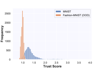
Figure 1: Comparing the distribution of Trust Scores for the test sets of (i) MNIST and (ii) FashionMNIST, CNN trained on MNIST.

(a) Query

(b) W-CF

(c) Proto-CF

(d) NUN-CF

Figure 2: Comparing Post-Hoc Counterfactual Explanations on MNIST for a Query Image: True Label = 5 & Predicted Label = 3. Three counterfactual explanations are of the form; “If the image looked like this, the system would have correctly classified it as a 5”. The counterfactual explanation produced by Proto-CF is quite uncertain (MC-Mean = 0.56, MC-STD = 0.30, Trust Score = 1.00), relative to the explanation produced by NUN-CF (MC-Mean = 0.99, MC-STD = 0.03, Trust Score = 1.18). See supplement for additional examples.

Results. Instances from the OoD FashionMNIST test set were found to have significantly lower trust scores compared to those from the original MNIST test set (Wilcoxon $p<0.01$), see Figure 1. Moreover, instances that were determined to be OoD by 10-LOF had significantly lower trust scores (mean = 0.971 $\pm$ 0.001) than those that were deemed to be within the data distribution (mean = 1.319 $\pm$ 0.004). These results indicate that trust scores can operate as a good proxy for OoD detection. Worryingly, many of the OoD instances were found to have high softmax probabilities, even if they had low-trust scores. For example, the CNN would often be $\approx 99\%$ sure an image of a shirt was actually an image of an eight, confirming that the softmax probabilities are a poor heuristic for detecting distributional shifts, whilst trust scores were more reliable. There is a strong monotonic relationship between MC-Mean and Trust Scores $r\approx 0.78$, indicating that trust scores are a useful proxy for uncertainty estimation in explanation. However, user studies will ultimately be needed to confirm these findings.

Experiment 2: Comparing Counterfactuals. In our next experiment, we generate and comparatively evaluate counterfactual explanations for misclassifications of a CNN classifier on MNIST. We monitor uncertainty in the explanation using MC-Dropout and compute the Trust Scores of the generated explanations. Where possible, we also visualise the explanation. We evaluate the explanations produced by several popular counterfactual techniques that can readily generate explanations for three different data types (tabular, image, and time series):

• NUN-CF (Nugent & Cunningham, 2005): This simple method retrieves the nearest neighbour to the query in a counterfactual class (nearest-unlike-neighbour).

• W-CF: Inspired by Wachter et al. (2017), this perturbation-based technique aims to generate sparse and proximal explanations by emulating the closest possible world.

• Proto-CF: Originally proposed by Klaise et al. (2020), this state-of-the-art method facilitates the implementation of an auto-encoder to aid the generation of plausible counterfactuals by maximizing the likelihood of $x^{\prime}$ under the training data distribution, following Dhurandhar et al. (2018). Class prototypes are used to guide and speed up the counterfactual generation process.

Results. We observe that explanations produced by Proto-CF (Van Looveren & Klaise, 2019) in the image domain are often quite ambiguous and blurry, confirming previous findings in other works (Schut et al., 2021; Kenny & Keane, 2021). The explanations are also quite uncertain according to MC-Dropout (MC-Mean $\approx$ $0.67$) and have relatively low trust scores (mean = 0.977 $\pm 0.008$), indicating that they poorly resemble instances in the training data of the counterfactual class.

W-CF produces explanations with almost identical trust scores to the originally misclassified instances. This is somewhat unsurprising as W-CF is prone to generating adversarial examples (Wachter et al., 2017), frequently resulting in explanations that are extremely similar to the test image, which are often not perceptibly different due to small pixel-level changes (Kenny & Keane, 2021) (see Fig.2).

On the other hand, explanations produced by NUN-CF are inherently well grounded in the training data (MC-Mean $\approx$ 0.93). Despite their simplicity, NUN-CF generates surprisingly good counterfactuals for MNIST misclassifications at the cost of sparsity and proximity. However, it is unclear how sparse or proximal good counterfactual explanations should be due to a lack of adequate user testing (Keane et al., 2021). Indeed, we note that explanations produced purely by NUN-CF are often not practical (e.g., when images are poorly aligned or less diverse training sets are available). However, such instances have been successfully used to guide counterfactual generation beyond MNIST in more complex color image datasets (Goyal et al., 2019), an inherently difficult problem for the XAI community.

4 Recommendations and Discussion

Providing uncertainty estimations on counterfactual explanations is a relatively unexplored yet immensely promising problem that can greatly aid the provision of trustworthy recourse (Bhatt et al., 2020; Schut et al., 2021). In light of this, we explore several practical solutions for quantifying uncertainty in counterfactual explanations. When explaining the predictions of neural networks we recommend using Monte Carlo dropout as a fast and efficient tool for determining uncertainty in explanation (Gal & Ghahramani, 2016; Kenny & Keane, 2021). We propose trust scores (Jiang et al., 2018) as a practical tool for evaluating how well explanations are grounded in the training data. Experiments demonstrate that trust scores provide a good proxy measure for uncertainty and for out-of-distribution detection. Moreover, unlike other popular techniques, trust scores make no assumptions about the model architecture or the availability of an auto-encoder and can also be readily extended to regression tasks (de Bie et al., 2021). For a deeper exploration of the promise of uncertainty estimation in XAI, we recommend the survey compiled by Bhatt et al. (2020) and the excellent technical report by Davis et al. (2020).

Extending these experiments to more complex image and time series datasets and exploring the role of adversarial training in providing robust recourse and uncertainty estimates is an interesting avenue for future work (Upadhyay et al., 2021; Schut et al., 2021). Motivated by the lack of user studies in counterfactual evaluation (Keane et al., 2021), it will be important to conduct extensive user tests to explore what users deem to be out-of-distribution and what computational proxy might best capture such cases.

Appendix A Supplementary Material

Black-box model.

For both experiments we train a convolutional neural network (CNN) as our black-box classifier following the architecture implemented by Van Looveren & Klaise (2019). Both MNIST (LeCun & Cortes, 2010) and FashionMNIST (Xiao et al., 2017) images are scaled to [-0.5,0.5] and the default training and test sets are used. Dropout layers are implemented for regularization and conveniently facilitate uncertainty computations using MC-Dropout. We train with an Adam optimizer for 10 epochs using a batch size of 256. The classifier achieves an accuracy of 98.93% on the MNIST test set leaving 107 to-be-explained images which are misclassified.

For a black-box classifier $b$, let $x$ be some to-be-explained instance with predicted class $y$, and $x^{\prime}$ be some candidate counterfactual explanation such that $b(x^{\prime})=y^{\prime}$.

Softmax Probability. Hendrycks & Gimpel (2017) suggest that as a simple baseline for OoD detection and uncertainty estimation in deep neural networks is to monitor the softmax probability i.e monitor $p(y|x,D)$ where D is the training distribution. For counterfactual explanations this amounts to determining $p(y^{\prime}|x^{\prime},D)$ (Schut et al., 2021).

Monte Carlo Dropout. We provide a brief overview of how MC-Dropout (Gal & Ghahramani, 2016) works, closely following the description by Davis et al. (2020). Once a predictive distribution $p(y|x,D)$ is obtained, the corresponding uncertainty can be uncovered by exploring the variance. In order to learn this distribution we can learn the parametric posterior distribution p($\Theta|D)$ (i.e., the distribution over the model parameters).

Gal & Ghahramani (2016) discovered that, by randomly switching off neurons in a neural network using different dropout configurations, one could approximate the parametric posterior distribution without the need to retrain the network. Each dropout configuration $\Theta_{t}$ corresponds to a sample from the approximate parametric posterior distribution $q(\Theta|D)$ s.t. $\Theta_{t}\sim q(\Theta|D)$.

Sampling from the approximate posterior enables us to uncover the predictive distribution $p(y|x)$:

$$p(y|x,D)\approx\int_{\Omega}\underbrace{p(y|x,\Theta)}_{likelihood}\underbrace{q(\Theta|D}_{posterior})\,d\Theta$$ (2)

The above integral can be approximated through Monte Carlo methods, yielding;

$$p(y|x,D)\underbrace{\approx}_{MC}\frac{1}{T}\sum_{t=1}^{T}p(y|x,\Theta_{t})$$ (3)

Indeed multiple forward passes with different dropout configurations allow us to uncover the predictive distribution. If we assume that likelihood is Gaussian distributed, the mean $f(x,\theta)$ and variance $s^{2}(x,\Theta)$ parameters of the Gaussian function are determined from the Monte Carlo simulations s.t $f(x,\theta),s^{2}(x,\Theta)\sim$ MC-Dropout(x), and can provide information about the predictive uncertainty through linking back with Equation 1.

$${\mathbb{V}(y|x)}=\underbrace{\mathbb{V}(\overbrace{\mathbb{E}(y|x,\Theta)}^{f(x,\theta)})}_{Epistemic}+\underbrace{{\mathbb{E}(\overbrace{\mathbb{V}(y|x,\Theta)}^{s^{2}(x,\Theta)})}}_{Aleatoric}$$ (4)

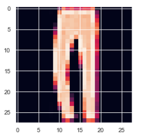
Figure 3: Softmax Deterministic Overconfidence; The black-box CNN classifier trained on MNIST images is 99.21 % sure this image of ‘trouser’ is an image of a ‘7’. Trust Score = 0.907.

Computing Trust Scores.

We compute trust scores using the implementation provided by (Klaise et al., 2020). We set $k=10$, so that 10 - nearest neighbours are considered for distance calculations. We set the distance type to $point$ such that the distance to the $k$-th nearest neighbour is computed when determining the trust score. A Euclidean distance metric is used, we set the filter parameter $\alpha$ = 0 with a leaf size of 40 for kd-trees.

While trust scores work best for low-mid dimensional datasets, the authors note that reducing dimensionality of complex datasets has negligible implications on the information conveyed by Trust Scores and can speed up computation (Jiang et al., 2018). We compute the trust scores for the images without any dimensionality reduction so that they can fairly be considered with MC-Dropout.

Interpreting Trust Scores. A trust score of 1 means that the distance to the predicted class is the same as the distance to the nearest other class. One way of interpreting why the OoD FashionMNIST images have trust scores close to one (mean = 0.971 $\pm$ 0.001) is because they equally do not particularly resemble any of the classes in the MNIST training set. Unsurprisingly, the trust scores of the MNIST class prototypes are much higher (mean = 1.56 $\pm$ 0.103).

Local Outlier Factor Method. The Local Outlier Factor Method (Breunig et al., 2000) was implemented as a novelty detector setting $k=10$ and using a Euclidean distance metric.

IM1 Omission.

IM1 (Van Looveren & Klaise, 2019) is a popular metric for evaluating the realism of counterfactual explanations, based on the reconstruction losses of auto-encoders. Realism can be linked to epistimitic uncertainty (Schut et al., 2021). We omit this metric from our evaluation for several reasons. Firstly, the metric requires separate auto-encoders to be trained on the to-be-explained and counterfactual class. For MNIST this would require training 10 separate auto-encoders that can successfully reconstruct the class (a non-trivial task). This is even more intractable for more complex datasets with more classes requiring even more autoencoders to be trained, where reconstruction of complex color images is much more difficult.

A.1 Counterfactual Methods

In this section we provide more information about the counterfactual methods used in Experiment 2.

Proto-CF. Originally proposed by Van Looveren & Klaise (2019), this method aims to generate a counterfactual by minimizing a multi-objective loss function;

$$Loss=cL_{pred}+\beta L_{1}+L_{2}+L_{AE}+L_{proto}$$ (5)

The first term in the loss function encourages the perturbed instance to belong to the counterfactual class. The elastic net regularizer $\beta L_{1}+L_{2}$ aims to ensure sparsity and proximity in the generated instance. $L_{AE}$ is the reconstruction error of the candidate counterfactual instance which is minimized to encourage the counterfactual to belong to the training data distribution. However, to specifically guide the instance towards the distribution of the perturbed class the $L_{2}$ distance between the instance and the counterfactual class prototype is minimized in the $L_{proto}$ term.

Following the recommendations of the authors we set hyperparameters; $\gamma$ = 100, $\Theta$ = 100, $c_{init}$ = 1, $c_{steps}$=2, and max iterations = 1000. We train a convolutional autoencoder following the architecture of Van Looveren & Klaise (2019) to facilitate the use of the $L_{AE}$ term.

W-CF. Inspired by Wachter et al. (2017), this technique aims to generate a counterfactual by emulating the closest possible world and is implemented in (Klaise et al., 2020). The counterfactual instance $x^{\prime}$ is generated through minimizing a simple loss function:

$$Loss=L_{pred}+\lambda L_{dist}$$ (6)

We set hyperparameters; target class = $other$, target proba = 0.5 to emulate an instance close to the decision boundary or possible world, tol = 0.01, $lam_{init}$ = 0.1, $lam_{steps}$=10, and max iterations = 1000. The Manhattan distance between the query and counterfactual is minimized in the loss function to generate sparse and proximal explanations.

NUN-CF. Originally proposed by Nugent & Cunningham (2005), this technique retrieves an explanation by locating the nearest neighbour in a counterfactual class. Alternatively, the target counterfactual class can be specified, which speeds up counterfactual retrieval as we consider a smaller pool of training images. Following Kenny & Keane (2021), we use a 1-nearest neighbour search across the pixel space using $L_{2}$ distance to retrieve neighbours.

Tabulated Results from Experiment 2.

Table 1: The average performance of counterfactual explanations generated by different techniques for MNIST misclassifications (107 in total) according to MC-Mean (higher is better), MC-STD (lower is better) and Trust Scores.

Method	MC-Mean	MC-STD	Trust Score
Proto-CF	0.667	0.242	0.977
W-CF	0.761	0.294	1.017
NUN-CF	0.931	0.115	1.180

(a) Query

(b) Proto-CF

(c) NUN-CF

Figure 4: Comparing counterfactual explanations generated by different methods for MNIST misclassifications.

References

- Adadi & Berrada (2018) Adadi, A. and Berrada, M. Peeking inside the black-box: a survey on explainable artificial intelligence (xai). IEEE access, 6:52138–52160, 2018.
- Bhatt et al. (2020) Bhatt, U., Antorán, J., Zhang, Y., Liao, Q. V., Sattigeri, P., Fogliato, R., Melançon, G. G., Krishnan, R., Stanley, J., Tickoo, O., et al. Uncertainty as a form of transparency: Measuring, communicating, and using uncertainty. arXiv preprint arXiv:2011.07586, 2020.
- Breunig et al. (2000) Breunig, M. M., Kriegel, H.-P., Ng, R. T., and Sander, J. Lof: identifying density-based local outliers. In Proceedings of the 2000 ACM SIGMOD international conference on Management of data, pp. 93–104, 2000.
- Byrne (2019) Byrne, R. M. Counterfactuals in explainable artificial intelligence (XAI): Evidence from human reasoning. In IJCAI-19, pp. 6276–6282, 2019.
- Davis et al. (2020) Davis, J., Zhu, J., Oldfather, J., MacDonald, S., and Trzaskowski, M. Quantifying uncertainty in deep learning systems - An Amazon Web Services Prospective. In AWS Prespictive Guidance Report, 2020. URL https://docs.aws.amazon.com/prescriptive-guidance/latest/ml-quantifying-uncertainty/welcome.html.
- de Bie et al. (2021) de Bie, K., Lucic, A., and Haned, H. To trust or not to trust a regressor: Estimating and explaining trustworthiness of regression predictions. arXiv preprint arXiv:2104.06982, 2021.
- Delaney et al. (2021) Delaney, E., Greene, D., and Keane, M. T. Instance-based counterfactual explanations for time series classification. In ICCBR-21. Springer, 2021.
- Dhurandhar et al. (2018) Dhurandhar, A., Chen, P.-Y., Luss, R., Tu, C.-C., Ting, P., Shanmugam, K., and Das, P. Explanations based on the missing: Towards contrastive explanations with pertinent negatives. In Advances in Neural Information Processing Systems, pp. 590–601, 2018.
- Gal (2016) Gal, Y. Uncertainty in deep learning. University of Cambridge, 1(3):4, 2016.
- Gal & Ghahramani (2016) Gal, Y. and Ghahramani, Z. Dropout as a bayesian approximation: Representing model uncertainty in deep learning. In international conference on machine learning, pp. 1050–1059. PMLR, 2016.
- Goyal et al. (2019) Goyal, Y., Wu, Z., Ernst, J., Batra, D., Parikh, D., and Lee, S. Counterfactual visual explanations. In International Conference on Machine Learning, pp. 2376–2384. PMLR, 2019.
- Guo et al. (2017) Guo, C., Pleiss, G., Sun, Y., and Weinberger, K. Q. On calibration of modern neural networks. In International Conference on Machine Learning, pp. 1321–1330. PMLR, 2017.
- Hendrycks & Gimpel (2017) Hendrycks, D. and Gimpel, K. A baseline for detecting misclassified and out-of-distribution examples in neural networks. Proceedings of International Conference on Learning Representations, 2017.
- Jesson et al. (2020) Jesson, A., Mindermann, S., Shalit, U., and Gal, Y. Identifying causal-effect inference failure with uncertainty-aware models. Advances in Neural Information Processing Systems, 33, 2020.
- Jiang et al. (2018) Jiang, H., Kim, B., Guan, M. Y., and Gupta, M. R. To trust or not to trust a classifier. In NeurIPS, pp. 5546–5557, 2018.
- Kanamori et al. (2020) Kanamori, K., Takagi, T., Kobayashi, K., and Arimura, H. Dace: Distribution-aware counterfactual explanation by mixed-integer linear optimization. In IJCAI-20, pp. 2855–2862, 2020.
- Karimi et al. (2020) Karimi, A.-H., Barthe, G., Balle, B., and Valera, I. Model-agnostic counterfactual explanations for consequential decisions. In International Conference on Artificial Intelligence and Statistics, pp. 895–905. PMLR, 2020.
- Karimi et al. (2021) Karimi, A.-H., Schölkopf, B., and Valera, I. Algorithmic recourse: from counterfactual explanations to interventions. In Proceedings of the 2021 ACM Conference on Fairness, Accountability, and Transparency, pp. 353–362, 2021.
- Keane & Smyth (2020) Keane, M. T. and Smyth, B. Good counterfactuals and where to find them: A case-based technique for generating counterfactuals for explainable ai (xai). In International Conference on Case-Based Reasoning, pp. 163–178. Springer, 2020.
- Keane et al. (2021) Keane, M. T., Kenny, E. M., Delaney, E., and Smyth, B. If only we had better counterfactual explanations: Five key deficits to rectify in the evaluation of counterfactual xai techniques. In IJCAI-21, 2021.
- Kendall & Gal (2017) Kendall, A. and Gal, Y. What uncertainties do we need in bayesian deep learning for computer vision? In Advances in Neural Information Processing Systems, volume 30, 2017.
- Kenny & Keane (2021) Kenny, E. M. and Keane, M. T. On generating plausible counterfactual and semi-factual explanations for deep learning. Proceedings of the AAAI Conference on Artificial Intelligence, 35(13):11575–11585, 2021.
- Klaise et al. (2020) Klaise, J., Van Looveren, A., Vacanti, G., and Coca, A. Alibi: Algorithms for monitoring and explaining machine learning models. URL https://github. com/SeldonIO/alibi, 2020.
- Lakshminarayanan et al. (2017) Lakshminarayanan, B., Pritzel, A., and Blundell, C. Simple and Scalable Predictive Uncertainty Estimation using Deep Ensembles. In Advances in Neural Information Processing Systems (NIPS 2017), volume 30, 2017.
- Laugel et al. (2019) Laugel, T., Lesot, M.-J., Marsala, C., Renard, X., and Detyniecki, M. The dangers of post-hoc interpretability: Unjustified counterfactual explanations. In IJCAI-19, pp. 2801–2807, 2019.
- LeCun & Cortes (2010) LeCun, Y. and Cortes, C. MNIST handwritten digit database. 2010. URL http://yann.lecun.com/exdb/mnist/.
- Lucic et al. (2020) Lucic, A., Haned, H., and de Rijke, M. Why does my model fail? contrastive local explanations for retail forecasting. In Proceedings of the 2020 Conference on Fairness, Accountability, and Transparency, pp. 90–98, 2020.
- Mahajan et al. (2019) Mahajan, D., Tan, C., and Sharma, A. Preserving causal constraints in counterfactual explanations for machine learning classifiers. In CausalML: Machine Learning and Causal Inference for Improved Decision Making Workshop, NeurIPS 2019, December 2019.
- McGrath et al. (2020) McGrath, S., Mehta, P., Zytek, A., Lage, I., and Lakkaraju, H. When does uncertainty matter?: Understanding the impact of predictive uncertainty in ml assisted decision making. arXiv preprint arXiv:2011.06167, 2020.
- Miller (2019) Miller, T. Explanation in artificial intelligence: Insights from the social sciences. Artificial intelligence, 267:1–38, 2019.
- Molnar et al. (2020) Molnar, C., Casalicchio, G., and Bischl, B. Interpretable machine learning – a brief history, state-of-the-art and challenges. In ECML PKDD 2020 Workshops, pp. 417–431. Springer, 2020.
- Nalisnick et al. (2019) Nalisnick, E., Matsukawa, A., Teh, Y. W., Gorur, D., and Lakshminarayanan, B. Do deep generative models know what they don’t know? In International Conference on Learning Representations, 2019.
- Nugent & Cunningham (2005) Nugent, C. and Cunningham, P. A case-based explanation system for black-box systems. Artificial Intelligence Review, 24(2):163–178, 2005.
- Ovadia et al. (2019) Ovadia, Y., Fertig, E., Ren, J., Nado, Z., Sculley, D., Nowozin, S., Dillon, J., Lakshminarayanan, B., and Snoek, J. Can you trust your model's uncertainty? evaluating predictive uncertainty under dataset shift. In Advances in Neural Information Processing Systems, volume 32, 2019.
- Papenmeier et al. (2019) Papenmeier, A., Englebienne, G., and Seifert, C. How model accuracy and explanation fidelity influence user trust. arXiv preprint arXiv:1907.12652, 2019.
- Poyiadzi et al. (2020) Poyiadzi, R., Sokol, K., Santos-Rodriguez, R., De Bie, T., and Flach, P. Face: feasible and actionable counterfactual explanations. In Proceedings of the AAAI/ACM Conference on AI, Ethics, and Society, pp. 344–350, 2020.
- Rabanser et al. (2019) Rabanser, S., Günnemann, S., and Lipton, Z. C. Failing loudly: An empirical study of methods for detecting dataset shift. In Advances in Neural Information Processing Systems, pp. 1394–1406, 2019.
- Rawal et al. (2020) Rawal, K., Kamar, E., and Lakkaraju, H. Can i still trust you?: Understanding the impact of distribution shifts on algorithmic recourses. arXiv preprint arXiv:2012.11788, 2020.
- Schulam & Saria (2017) Schulam, P. and Saria, S. Reliable decision support using counterfactual models. In Advances in Neural Information Processing Systems (NIPS 2017), volume 30, pp. 1696–1706, 2017.
- Schut et al. (2021) Schut, L., Key, O., Mc Grath, R., Costabello, L., Sacaleanu, B., Gal, Y., et al. Generating interpretable counterfactual explanations by implicit minimisation of epistemic and aleatoric uncertainties. In Proc. International Conference on Artificial Intelligence and Statistics, pp. 1756–1764. PMLR, 2021.
- Upadhyay et al. (2021) Upadhyay, S., Joshi, S., and Lakkaraju, H. Towards robust and reliable algorithmic recourse. arXiv preprint arXiv:2102.13620, 2021.
- Ustun et al. (2019) Ustun, B., Spangher, A., and Liu, Y. Actionable recourse in linear classification. In Proceedings of the Conference on Fairness, Accountability, and Transparency, pp. 10–19, 2019.
- Van Looveren & Klaise (2019) Van Looveren, A. and Klaise, J. Interpretable counterfactual explanations guided by prototypes. arXiv preprint arXiv:1907.02584, 2019.
- Wachter et al. (2017) Wachter, S., Mittelstadt, B., and Russell, C. Counterfactual explanations without opening the black box: Automated decisions and the gdpr. Harv. JL & Tech., 31:841, 2017.
- Xiao et al. (2017) Xiao, H., Rasul, K., and Vollgraf, R. Fashion-mnist: a novel image dataset for benchmarking machine learning algorithms. arXiv preprint arXiv:1708.07747, 2017.