A Gemini–NIFS view of the merger remnant NGC 34
Abstract
The merger remnant NGC 34 is a local luminous infrared galaxy (LIRG) hosting a nuclear starburst and a hard X-ray source associated with a putative, obscured Seyfert 2 nucleus. In this work, we use adaptive optics assisted near infrared (NIR) integral field unit observations of this galaxy to map the distribution and kinematics of the ionized and molecular gas in its inner , with a spatial resolution of 70 pc. The molecular and ionized gas kinematics is consistent with a disc with projected major axis along a mean PA = . Our main findings are that NGC 34 hosts an AGN and that the nuclear starburst is distributed in a circumnuclear star-formation ring with inner and outer radii of 60 and 180 pc, respectively, as revealed by maps of the and emission-line ratios, and corroborated by PCA Tomography analysis. The spatially resolved NIR diagnostic diagram of NGC 34 also identifies a circumnuclear structure dominated by processes related to the stellar radiation field and a nuclear region where and H2 emissions are enhanced relative to the hydrogen recombination lines. We estimate that the nuclear X-ray source can account for the central H2 enhancement and conclude that and H2 emissions are due to a combination of photo-ionization by young stars, excitation by X-rays produced by the AGN and shocks. These emission lines show nuclear, broad, blue-shifted components that can be interpreted as nuclear outflows driven by the AGN.
keywords:
galaxies: individual: (NGC 34, NGC 17, Mrk 938) – galaxies: starburst – galaxies: nuclei – galaxies: ISM – infrared: galaxies1 Introduction
Local Universe galaxies display a wide range of luminosities, sizes, gas and stellar distribution and kinematics, that are the outcome of a process that lasts 13.8 Gyr. In the hierarchical scenario of galaxy formation and evolution, early-type galaxies form as a result of the merger of spiral galaxies whose discs are disrupted as the merging evolves (e.g.: White & Rees 1978; Hopkins et al. 2008; Deeley et al. 2017). In cases where the interacting galaxies are gas-rich (‘wet-merger’), the migration of vast amounts of gas towards the innermost regions of the merging system can lead to the onset of starbursts and/or active galactic nuclei (AGN) phenomena. However, this poses several challenges for the understanding of the fate of the interacting gas during these galaxies encounters; at the same time that gas is required either to form stars or to feed the AGN, it can also be expelled from the merger remnant by galactic winds related with these processes. Moreover, it is well known that star formation (SF) on galactic scales may be quenched, suppressed or triggered as a result of the AGN feedback (Harrison, 2017), thus raising the question if the AGN feeding happens simultaneously with the SF (Kawakatu & Wada, 2008), follows it during a post-starburst phase (Davies et al., 2007; Riffel et al., 2009) or lack any association with recent SF (Sarzi et al., 2007).
Luminous and Ultra Luminous Infrared Galaxies (LIRGs and ULIRGs, respectively) emit the bulk of their energy in the infrared (IR). For LIRGs, IR luminosities are in the range , while for ULIRGs, (Sanders et al., 2003). These objects harbor a strong nuclear starburst and/or an AGN (Sanders & Mirabel, 1996; Lonsdale et al., 2006), and most of local ULIRGs, and LIRGs with are often associated with gas-rich merging systems (Hung et al. 2014, for a recent review on the properties of LIRGs, see Pérez-Torres et al. 2021). Therefore, these objects have become increasingly important for galaxy evolution studies since they provide a laboratory for understanding the starburst/AGN feedback processes that shape the evolution of a merger remnant. The main power source of U(LIRGs) is the heating of dust by a starburst and/or an AGN, but the relative contribution of each process to the observed IR luminosities is still under debate. This happens mainly due to difficulties in carrying out high resolution optical/IR studies of these objects as a consequence of the heavy dust obscuration towards their nuclear regions and to the fact that they are more numerous at (Sanders & Mirabel, 1996; Lonsdale et al., 2006). Therefore, it is clear that in order to map in detail their stellar and gas properties, it is necessary to search for local prototypes of the (U)LIRGs population. Observations indicate that, at least for local LIRGs, the bulk of their IR luminosites is dominated by starburst emission (Alonso-Herrero et al., 2012), and that the AGN contribution to the observed IR luminosities increases with the IR luminosity of the system, and may dominate the energy budget for objects with (Nardini et al., 2010; Veilleux et al., 2009).
The galaxy NGC 34 (NGC 17, Mrk 938), (Rothberg & Joseph, 2006) and at a distance of (), is a local representative of the LIRGs class (, Chini et al. 1992). It hosts a dominant central starburst (e.g.: Riffel et al. 2006; Schweizer & Seitzer 2007; Riffel et al. 2008b; Dametto et al. 2014) with inferred star formation rates (SFR) in the range 50–90 (Valdés et al., 2005; Prouton et al., 2004). However, evidence on AGN activity has been extensively debated. Based on near-infrared (NIR) studies in the range 0.8–2.4 , Riffel et al. (2006) found that NGC 34 displays a poor emission-line spectrum and that the continuum emission is dominated by stellar absorption features. Therefore, they classified NGC 34 as a starburst galaxy. In the optical domain, Mulchaey et al. (1996) carried out an imaging survey of the and emission lines for a sample of early-type Seyfert galaxies and found that NGC 34 not only is a week emitter compared to most of the Seyferts in their sample, but also that emission is strong over the entire galaxy, indicating that the gas ionization is not related to any AGN. However, Yuan et al. (2010) and Brightman & Nandra (2011b) used Baldwin, Phillips and Terlevich (BPT) diagnostic diagrams (Baldwin et al., 1981; Kewley et al., 2001, 2006) to confirm that NGC 34 hosts a Seyfert 2 nucleus. Despite the highly controversial nature of the NGC 34 nuclear spectrum, X-ray observations provide compelling evidence for the presence of an obscured AGN in its central regions (e.g.: Guainazzi et al. 2005; Brightman & Nandra 2011a; Esquej et al. 2012). Esquej et al. (2012) found that the NGC 34 X-ray luminosity in the 2–10 keV energy range ( is too high to be solely due to the nuclear starburst, and is, therefore, dominated by an AGN.
The detailed study of the optical morphological properties of NGC 34 presented by Schweizer & Seitzer (2007) shows that this galaxy features a red nucleus, with a nuclear starburst confined to a radius 1 kpc; a young and blue central exponential disc at a position angle (PA) of -9∘, a system of young massive star clusters and a pair of unequal tidal tails indicative of the merger of two former gas-rich disc galaxies. In addition, Schweizer & Seitzer (2007) also reported that blueshifted Na i D lines reveal that the inner regions of NGC 34 drive a strong outflow of cool, neutral gas with a mean velocity of that could be due to the concentrated starburst and/or the hidden AGN.
The galaxy NGC 34 has also been probed in the radio and submillimetre regimes. Fernández et al. (2010) used 21 cm Very Large Array (VLA) observations to map the radio continuum emission and the H i distribution and kinematics. They found that the radio continuum emission structure consists of an extended nuclear component that is dominated by the central starburst, and an outer, extra–nuclear diffuse extended component in the shape of two radio lobes that could be evidence for past AGN activity or due to a starburst-driven super-wind. The authors detected a broad H i absorption profile with both blue-shifted and red-shifted velocities that could be explained by the presence of a circumnuclear disc (CND) of neutral and molecular gas. The existence of the CND was later confirmed by Fernández et al. (2014). They detected a rotating CO disc of 2.1 kpc in diameter using Combined Array for Research in Millimeter-wave Astronomy (CARMA) observations of the CO(1-0) transition at 115 GHz. An even more compact molecular rotating disc with a size of 200 pc was later detected by Xu et al. (2014) using Atacama Large Millimeter Array (ALMA) observations of the CO(6-5) emission line (rest-frame frequency = 691.473 GHz).
Finally, Mingozzi et al. (2018) used archival Herschel and ALMA observations of multiple CO transitions along with X-ray data from NuSTAR and XMM-Newton to perform the modelling of the CO Spectral Line Energy Distribution (SLED) - that is, the modelling of the luminosities of the CO lines as a function of their upper rotational levels. They found that a combination of a cold and diffuse photo-dissociation region (PDR) to account for the low-J transitions and a warmer and denser X-ray dominated region (XDR) to account for the high-J transitions was necessary to properly fit the CO line luminosities, and concluded that AGN contribution is significant in heating the molecular gas in NGC 34.
In this work, we use adaptive optics (AO) assisted NIR integral field unit (IFU) observations of the galaxy NGC 34 to map the distribution and kinematics of the ionized and molecular gas distributed in the inner . Our main goal is to investigate the nature of the NGC 34 NIR emission line spectrum in order to put tighter constraints on the presence of an AGN in its centre. Starburst phenomena, as in the case of NGC 34, are known for residing in dusty systems, therefore NIR observations are ideally suited for probing the central regions of these objects since they can pierce through highly obscured regions.
This paper is structured as follows. In Sec. 2 we present the observations and data reduction procedures, in Sec. 3 we describe our data analysis. Our results are shown in Sec. 4 followed by the discussion in Sec. 5. We summarise our findings in Sec. 6. At the redshift of , 1 corresponds to 411 pc for the adopted cosmology: , and (Planck Collaboration et al., 2020). The NGC 34 systemic velocity is .
2 Observations and Data Reduction
Data for this work were obtained with the Near-Infrared Integral Field Spectrograph (NIFS) of the Gemini North Telescope under the Gemini Science Programme GN-2011B-Q-71 (PI: Rogério Riffel) using the ALTitude conjugate Adaptive optics for the InfraRed (ALTAIR) system. The NIFS instrument provides a field of view (FoV) of that is sampled by spatial pixels (spaxels) with dimensions of as a result of its optical and geometrical properties.
Observations of NGC 34 were carried out in 2011 September 09 and 24 in the Kl (1.99–2.40) and J (1.15–1.33) bands, respectively. Eight on target (T) and four sky (S) exposures of 350 s were obtained in each band following the sequence TST. Observations of standard stars for telluric absorption removal and flux calibration, as well as flat-field, darks, Ronchi-flat and arc-lamp (Ar and ArXe for the J and Kl bands, respectively) were obtained for the data reduction process. The spectral resolution for both bands is 20 as measured by the full width at half maximum (FWHM) of the Ar and ArXe lines.
The data reduction was performed using the iraf (Image Reduction and Analysis Facility) environment along with standard reduction scripts made available by the Gemini team. The data reduction process includes the trimming of the images, sky subtraction, flat-field, bad pixel and spatial distortion corrections, wavelength calibration, telluric absorption removal and flux calibration by fitting a blackbody function to the spectrum of the telluric standard star. Individual reduced data cubes were constructed with spaxels of and were median combined in each band to a single data cube.
Fully calibrated and redshift corrected data cubes were obtained following the treatment procedures for Gemini–NIFS data cubes presented by Menezes et al. (2014), including the re-sampling of the image to spaxels with dimensions . High-frequency spatial noise was removed using a Butterworth filter with a cut-off frequency of 0.22 (where is the Nyquist frequency) for the J-band cube and 0.33 for the K-band cube, both with a filter order . Then, we removed low-frequency instrumental fingerprints using Principal Component Analysis Tomography (Steiner et al., 2009).
Our final data cubes have FoV’s of corresponding to at the galaxy, and spectral ranges of 1.128–1.310 and 2.081–2.370 in the J and K bands, respectively. The spatial resolution corresponding to the FWHM of the brightness profile of the telluric standard star is 0.17 () for both the J and K bands.
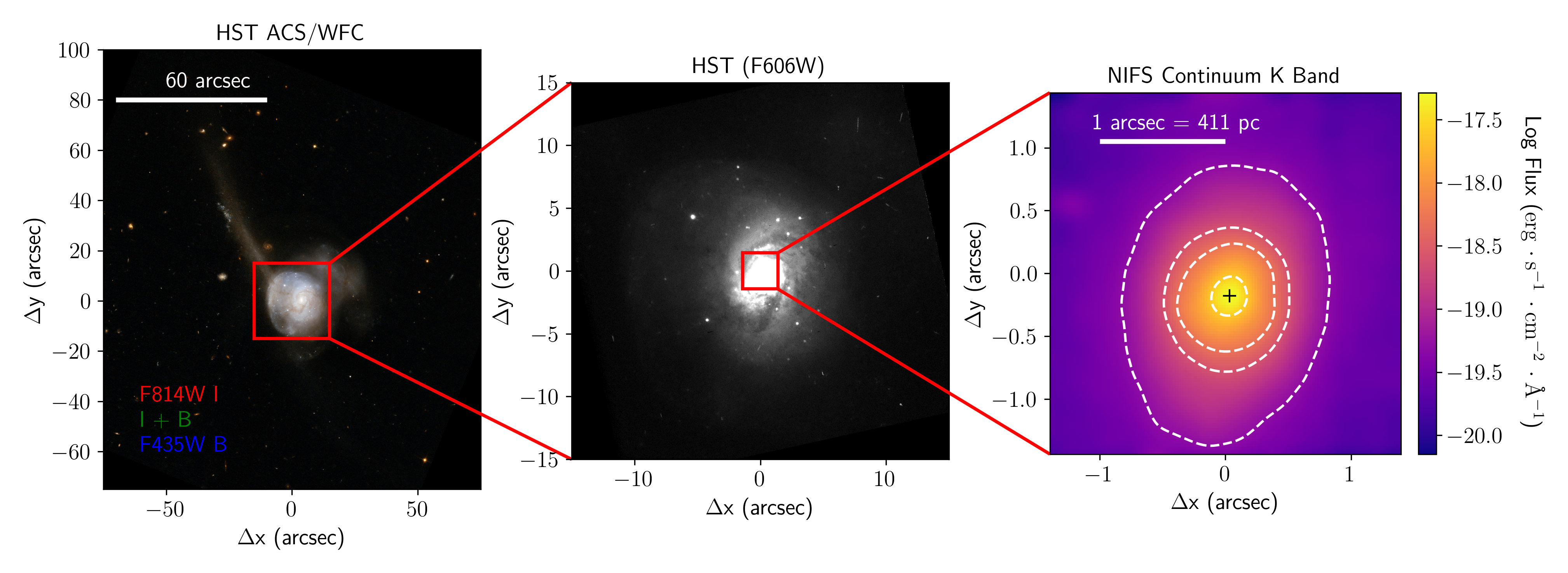
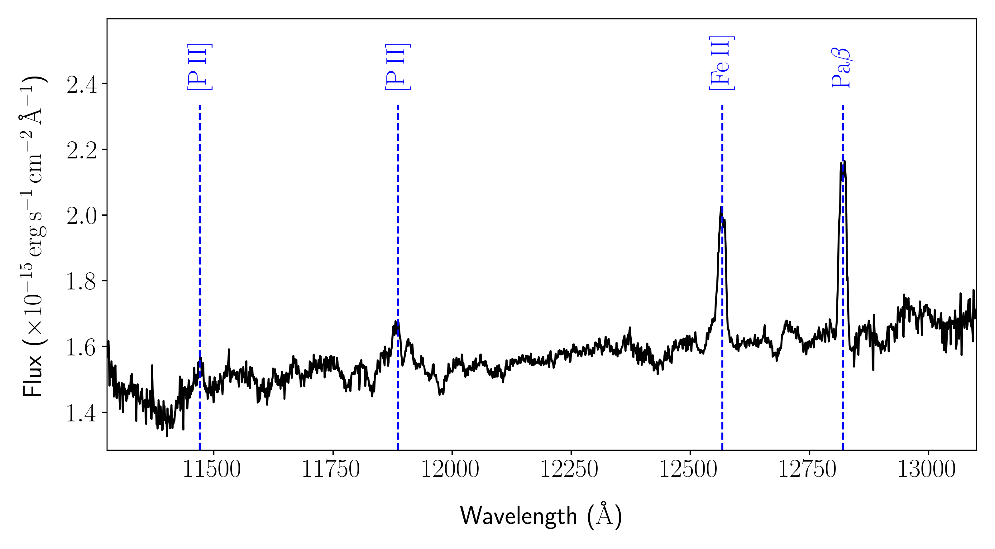
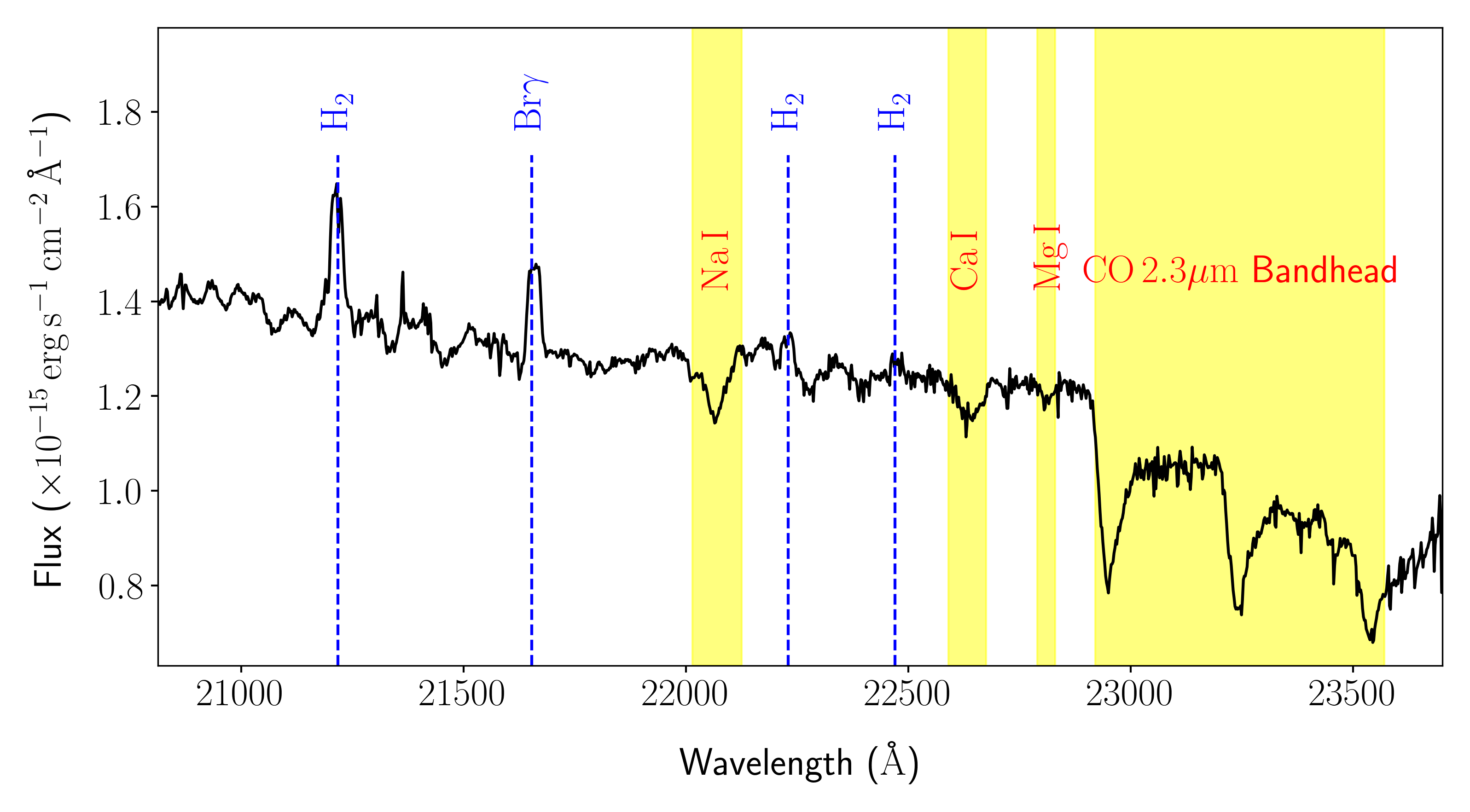
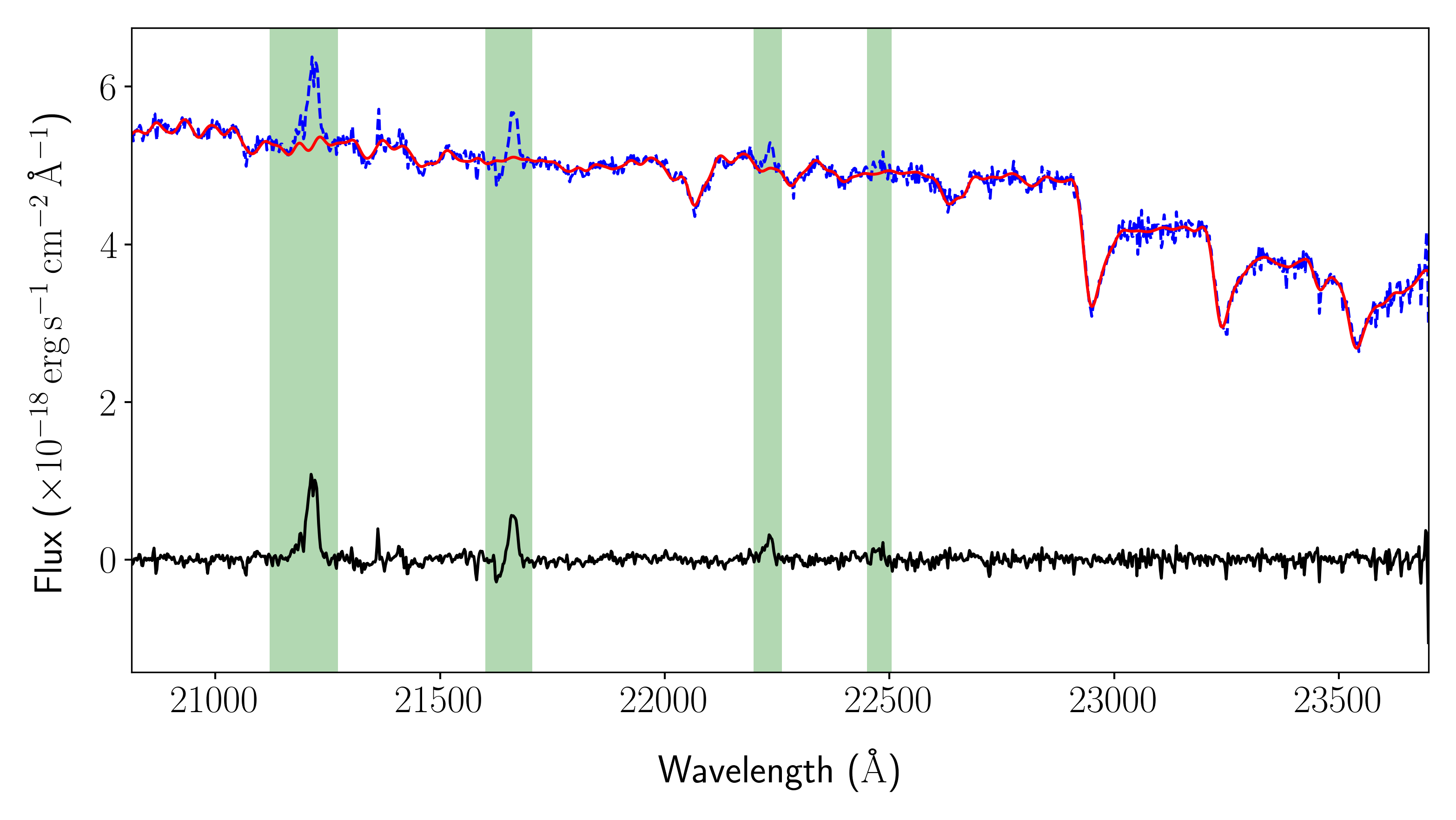
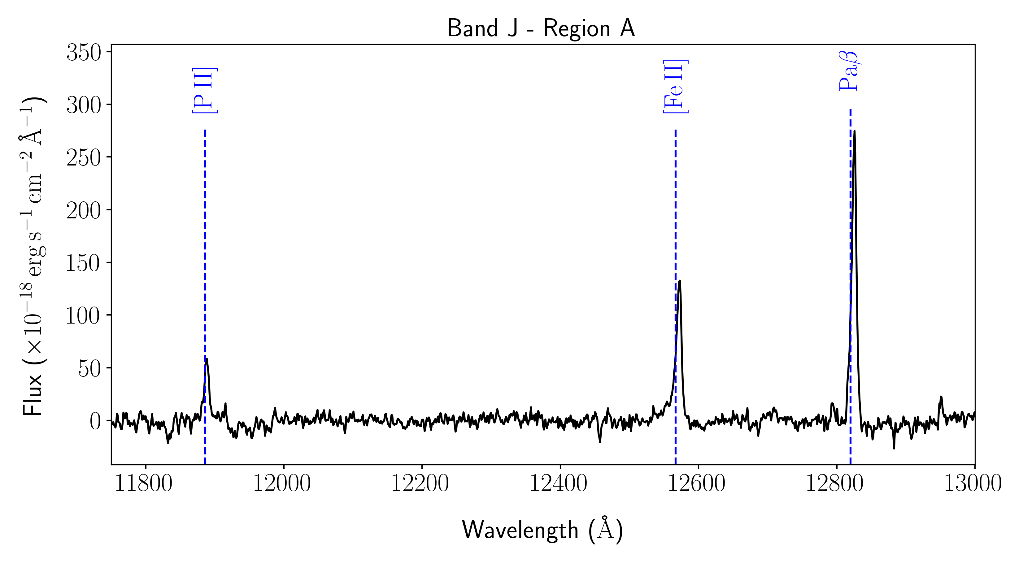
In the top-left panel of Fig. 1, we show an image of NGC 34 obtained by the Advance Camera for Surveys/Wide Field Camera (ACS/WFC) on board of the Hubble Space Telescope (HST) with the filters F814W and F435W. We show in the middle panel of Fig. 1 an HST Wide Field and Planetary Camera 2 (WFPC2) image of NGC 34 obtained with the filter F606W (Malkan et al., 1998) along with a K-band NIFS continuum image obtained from the average flux in the 2.180–2.195 wavelength range (top-right). Integrated NIFS J and K bands spectra over the entire FoV are shown in the bottom panels of Fig. 1. In the J band, the main NIR emission lines that can be seen in our spectra are Å , Å , Å and . In the K band, the Å , , Å and Å emission lines can be seen, in addition to the Na i 2.20, Ca i 2.26, Mg i 2.28 and CO 2.3 absorption features.
3 Data Analysis
3.1 Spectral synthesis
In order to study the nature of the gas emission lines present in the observed spectra of active/starburst galaxies, first, one needs to obtain spectra that are free from contamination caused by other components of the galaxy, such as the stellar population, dust content and AGN continuum (accretion disc). This is usually done through the application of the spectral synthesis technique, which requires a base of theoretical and/or empirical stellar spectra models to account for the other galaxy components and a code that quantifies the contribution of all these elements to the observed spectra. In this work, we used the NASA InfraRed Telescope Facility (IRTF) Spectral Library (Cushing et al., 2005; Rayner et al., 2009) and the Penalized Pixel-Fitting (ppxf, Cappellari 2017) code to obtain pure emission line (gas) spectra for the galaxy NGC 34 at the J and K bands.
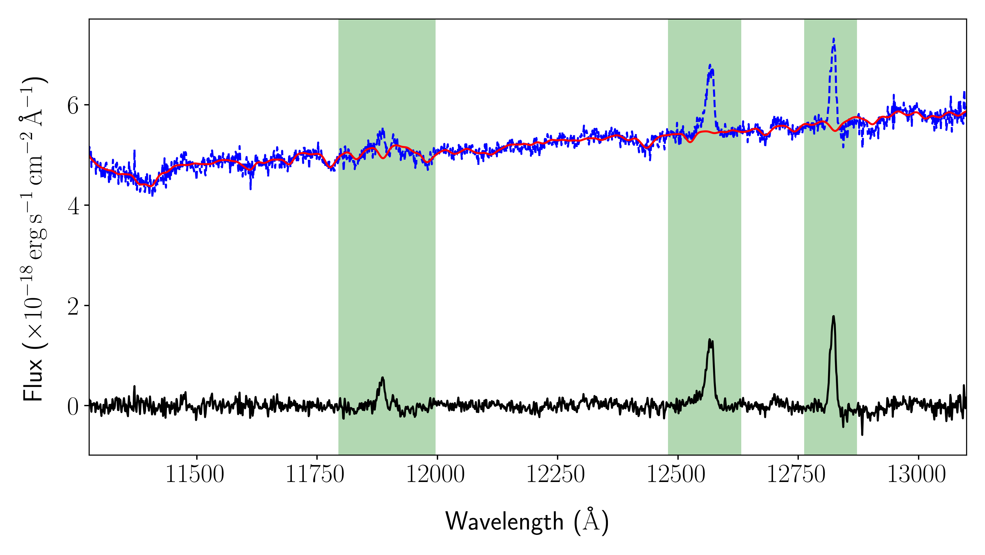
The IRTF Spectral Library () contains observed spectra in the 0.8–5 wavelength range for 210 cool stars, with mostly near-solar metallicities, and spectral types between F and M and luminosity classes between I and V, in addition to some AGB, carbon, and S stars (see Riffel et al., 2015, for a similar application). We used this set of observed spectra as an input template for the ppxf package to fit the continuum of the NGC 34 observed spectra in every spaxel of the data cubes. The fitting was performed separately for the J and K bands and the emission lines were masked before the fit. The stellar features were fitted using Gauss-Hermite profiles and we used only multiplicative polynomials to prevent changes in the line strength of the absorption features in the templates as recommended by Cappellari (2017). Examples of the gas spectra obtained following this procedure are shown in Fig. 2 for the J and K bands at the spaxel corresponding to the nucleus of the galaxy.
3.2 Emission-line fitting
We fitted the profiles of the emission lines using the package ifscube (Ruschel-Dutra & de Oliveira, 2020), which is a python based package designed to carry out analysis of data cubes of integral field spectroscopy. ifscube provides a set of tasks that allows the simultaneous fitting by multiple Gaussian curves or Gauss-Hermite series emission line profiles in velocity space. It also provides a Monte-Carlo implementation to estimate fitting uncertainties pixel-by-pixel.
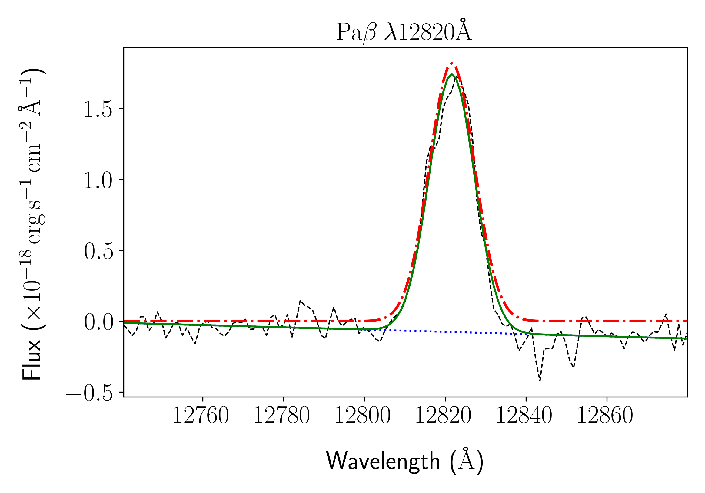
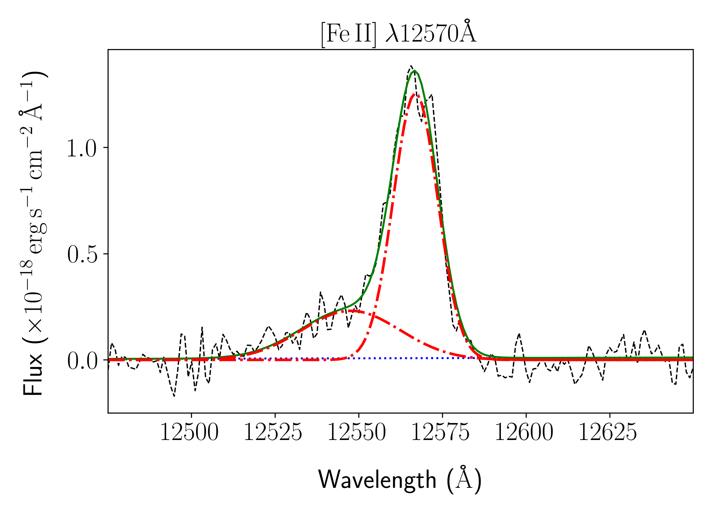
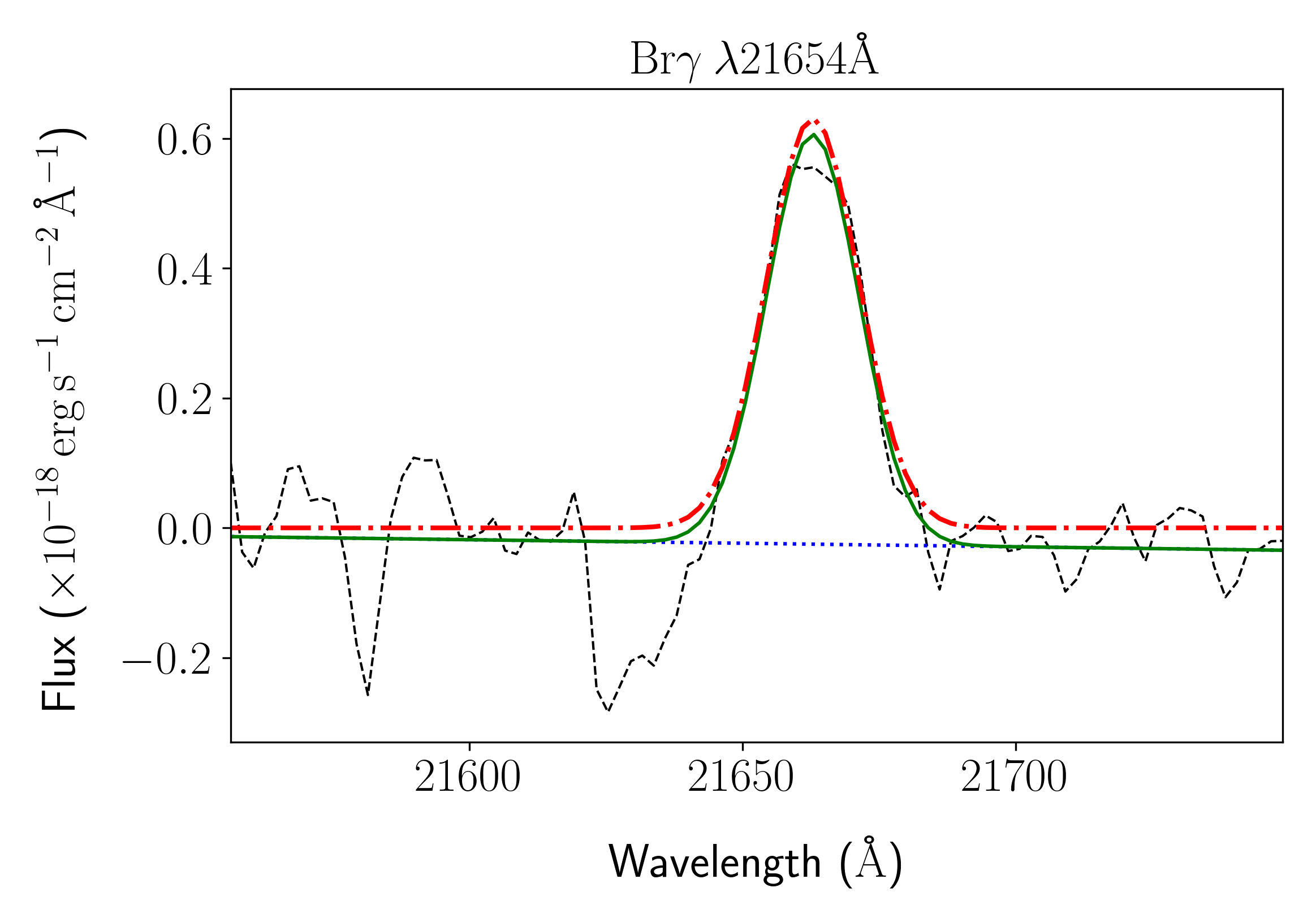
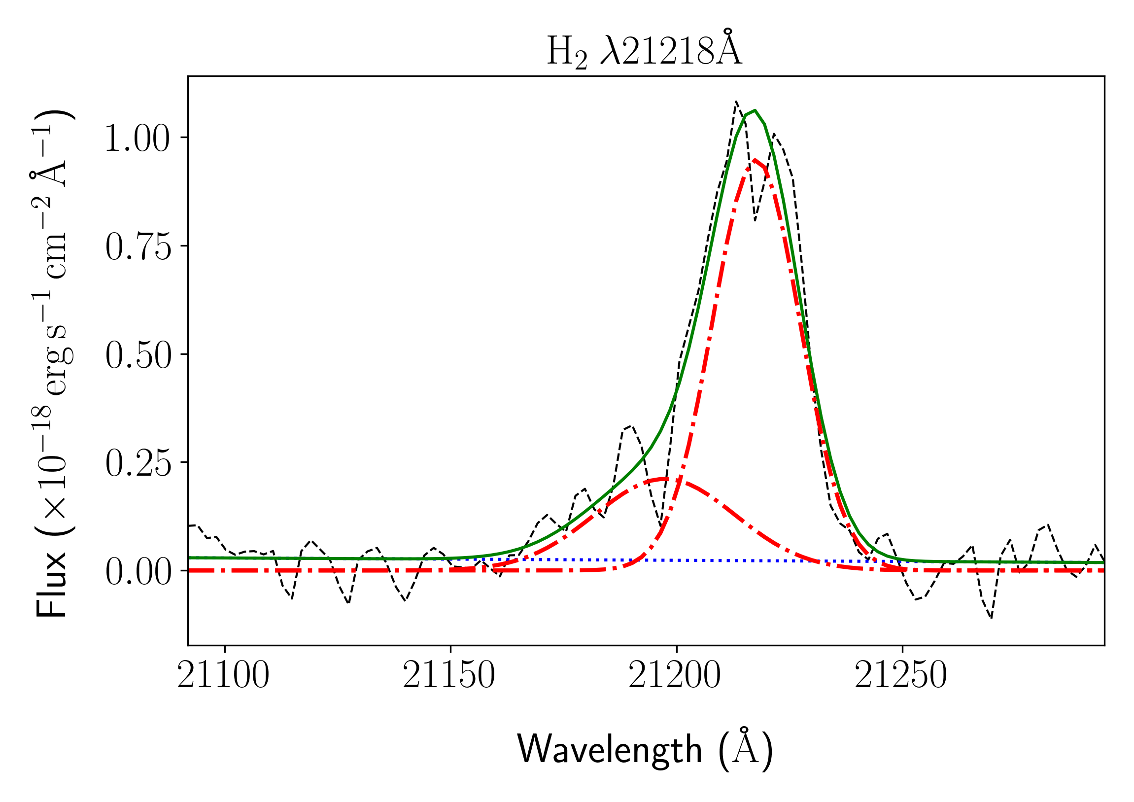
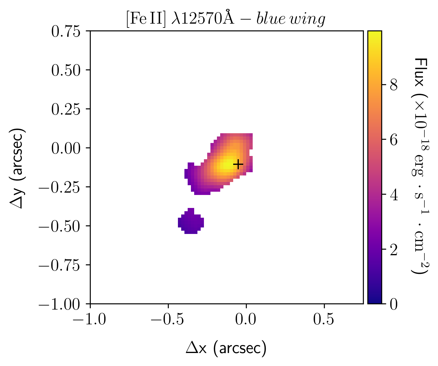
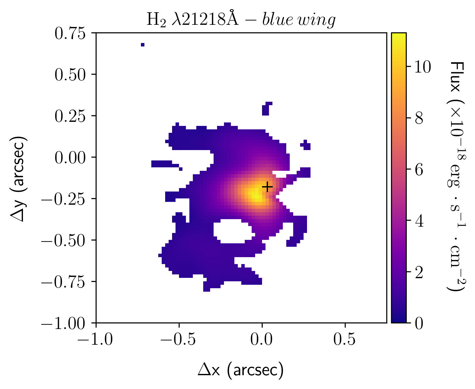
We used Gaussian functions to fit separately, in individual ifscube runs, each one of the emission lines seen in Fig. 1, thus obtaining their amplitudes, radial velocities, velocity dispersion () and integrated fluxes. Pixels where the peak of a given emission line compared to the standard deviation of the adjacent continuum was smaller than five were masked during the fit. We also included a one degree polynomial to account for the contribution of the underlying residual continuum to the observed emission. The Å , , , Å and Å emission lines were well fitted by a single Gaussian component. In the cases of the Å and Å emission lines, we started by fitting them with a single Gaussian, however this procedure was not able to account for the presence of broad, blue wings in a region of radius around the nucleus of the galaxy, therefore we included a second Gaussian to fit their profiles. We fixed the radial velocities of these components at and and their velocity dispersions at 350 and 215 for the Å and Å emission lines, respectively, as determined from the fitting of the nuclear spectra, integrated in an aperture of 0.20.2, also using the package ifscube. However, since these components are fitted simultaneously with their main narrow counterparts, a further threshold needs to be applied to claim their detection (see Sec. 4.1). We note that we did not detect broad, blue-shifted components associated with the other H2 emission features. This could be due to the fact the H2 emissions at Å and Å are much weaker compared to the emission at Å or a result of different excitation mechanisms of the H2 molecule, as will be discussed in Sec. 5.3.
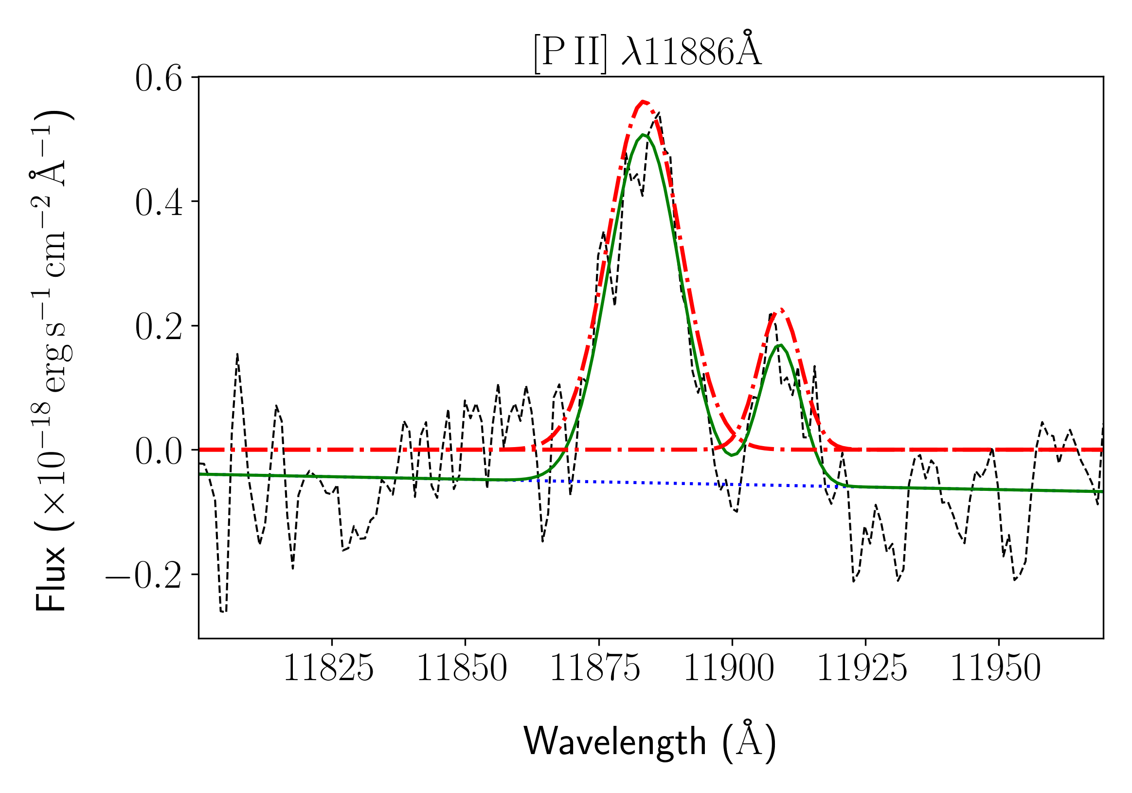
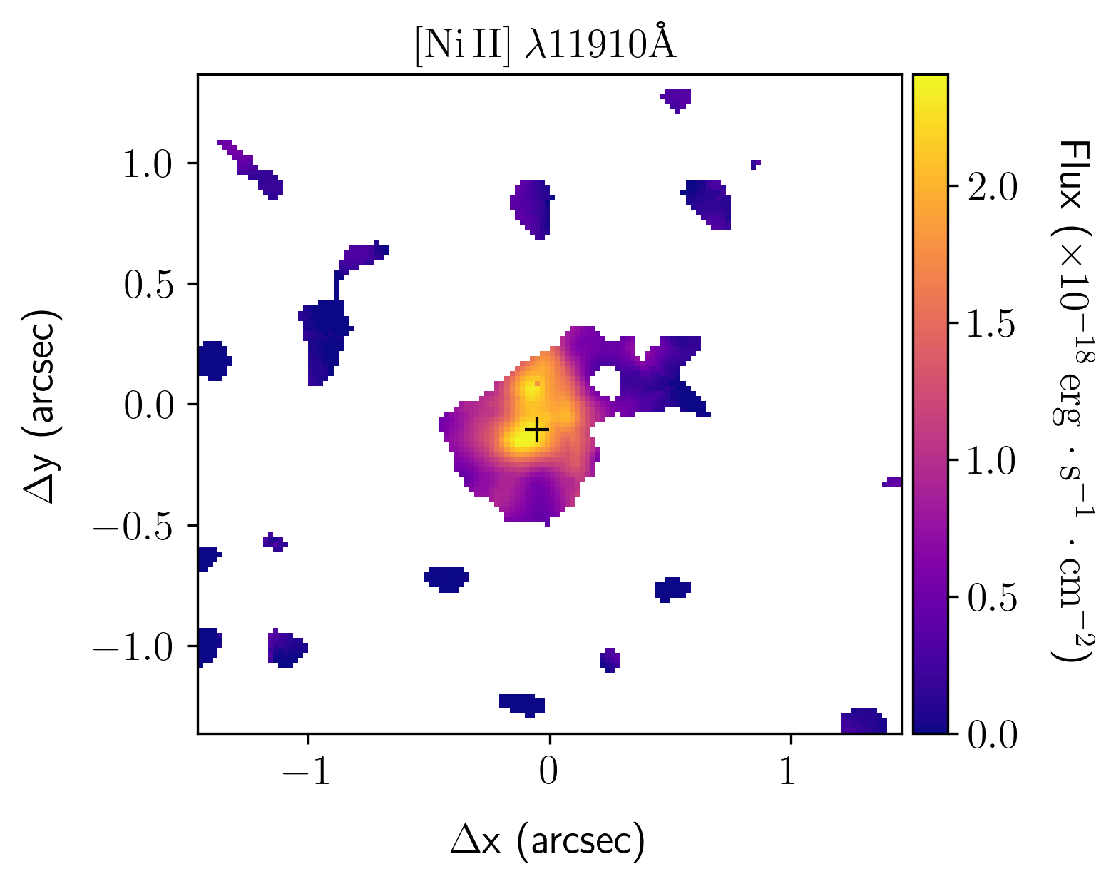
We point out that while fitting the Å emission line, we noticed a neighbouring emission feature at the wavelength 11910 Å corresponding to a forbidden transition of . For this reason, we fitted these lines simultaneously, although we kept their kinematics independent. The Å emission is confined to a region of radius smaller than 0.3 in the centre of o the FoV and it does not affect the fitting of the Å profile.
We show in Fig. 3 the resulting fits for the main emission lines for the spaxel corresponding to the nucleus of the galaxy. From these example fits, one can see that the broad, blue-shifted components accompanying the Å and Å emission lines are clearly distinguished from their main narrow counterparts. Moreover, the panel displaying the resulting fit for the Å emission line also shows a second, well separated feature corresponding to the Å emission. We did not attempt to model the emission at Å since it is barely seen in the integrated spectra show in Fig. 1 as well as in the gas spectra shown in Fig. 2.
4 Results
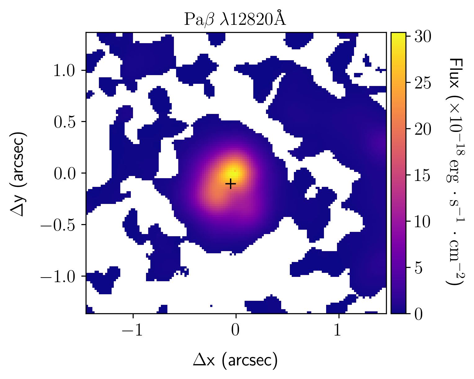
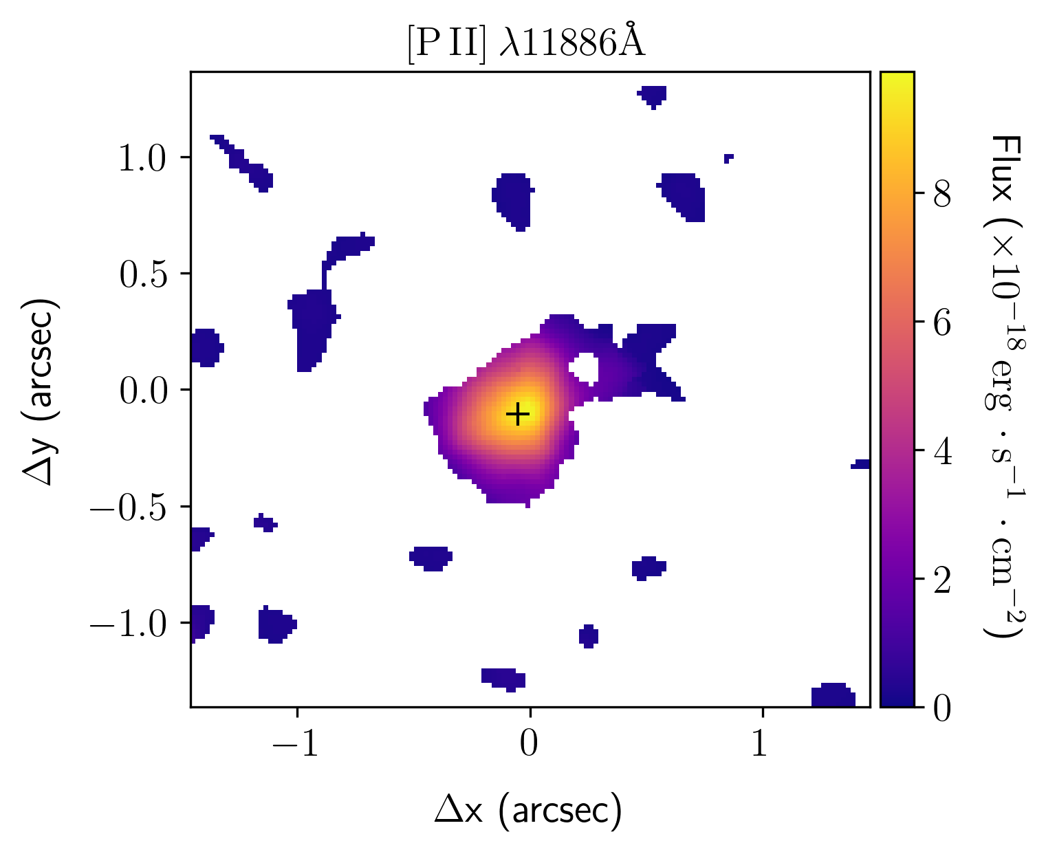
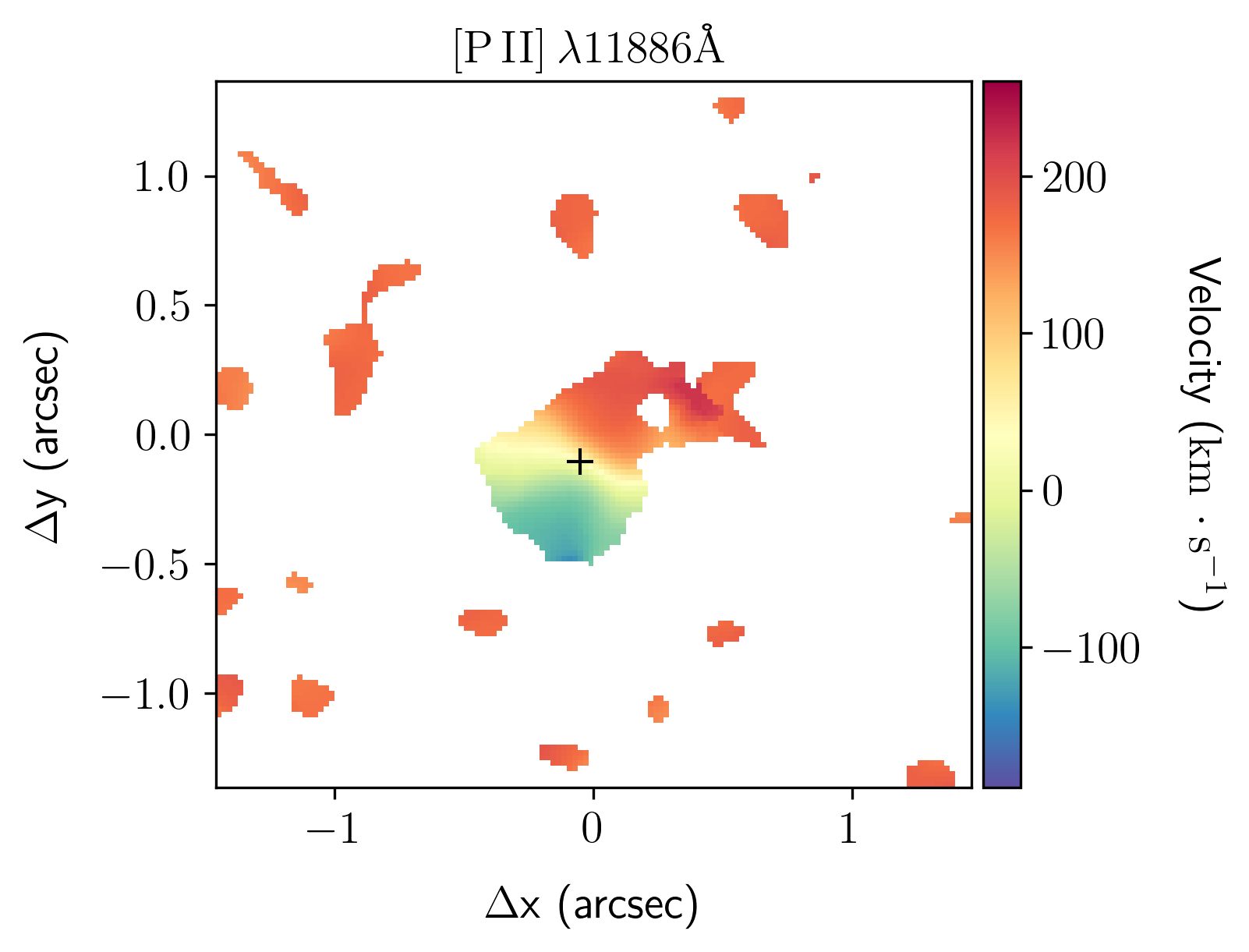
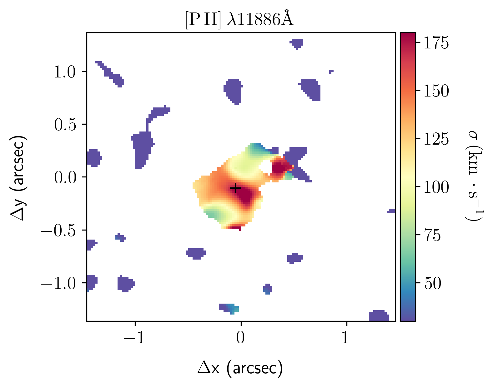
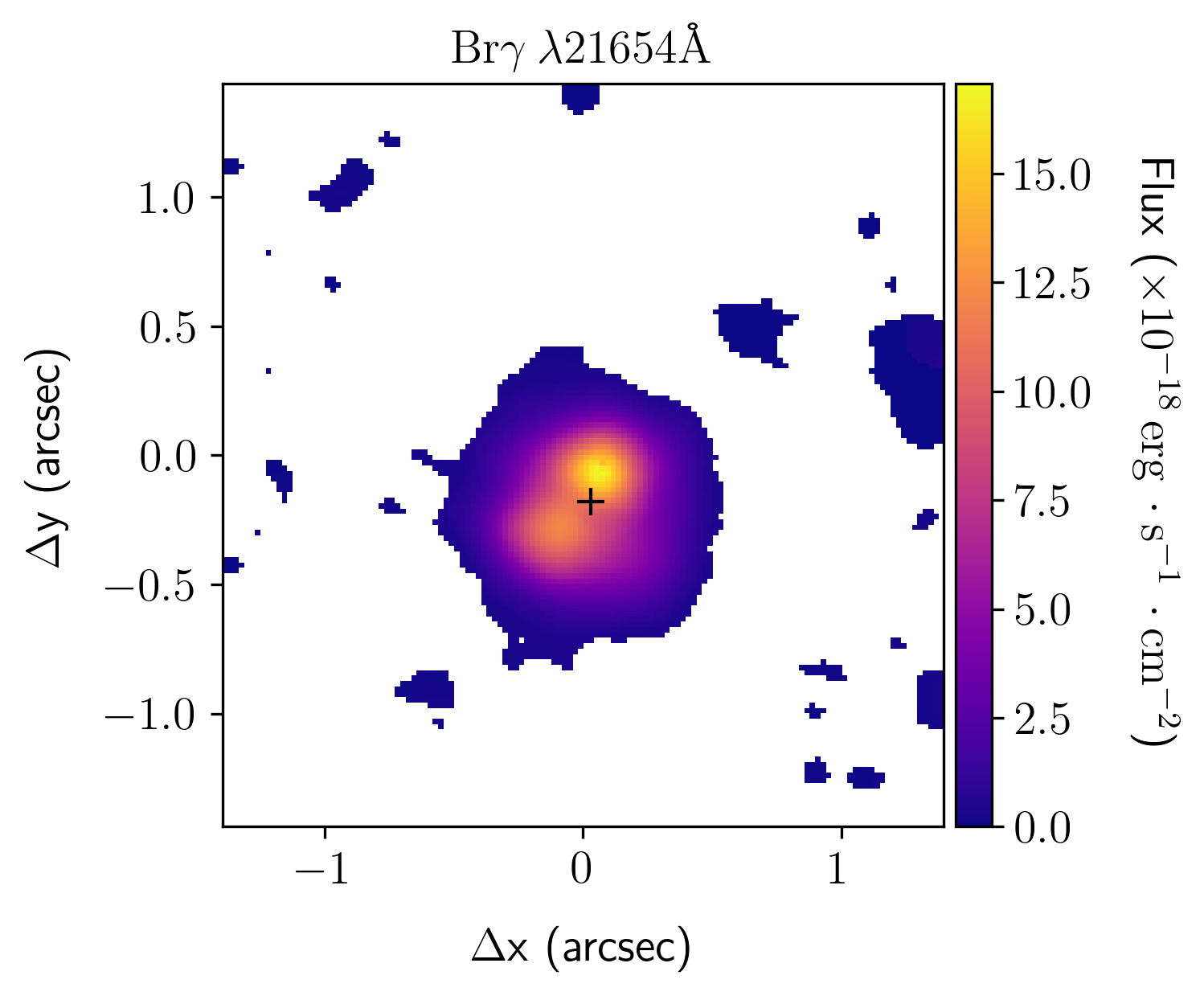
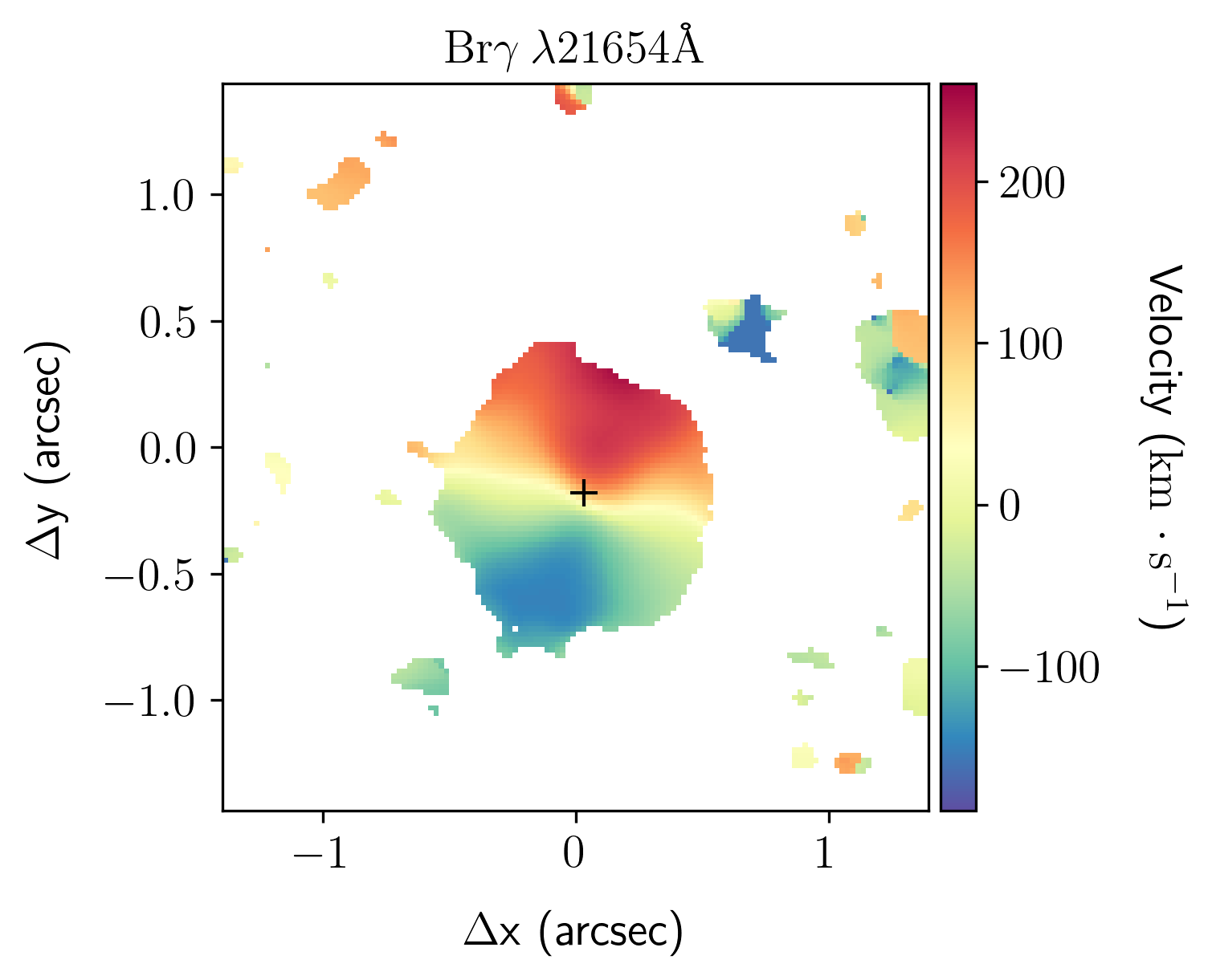
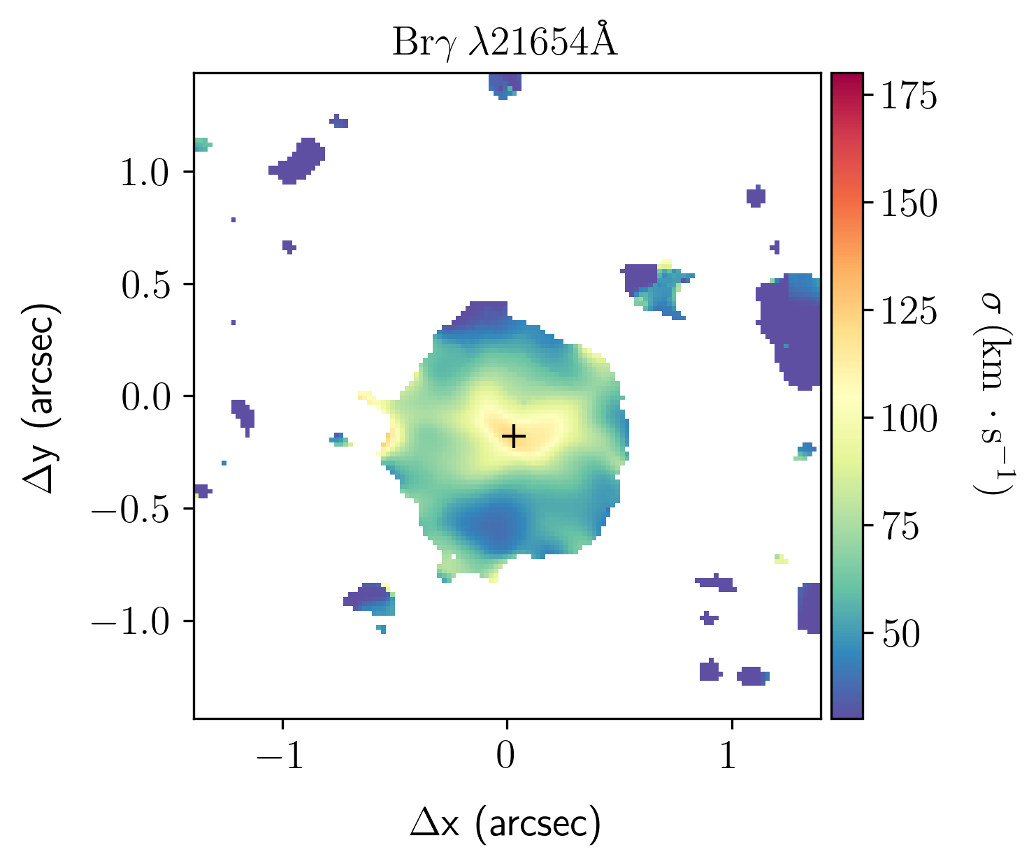
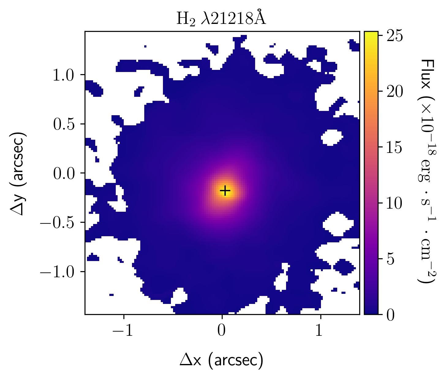
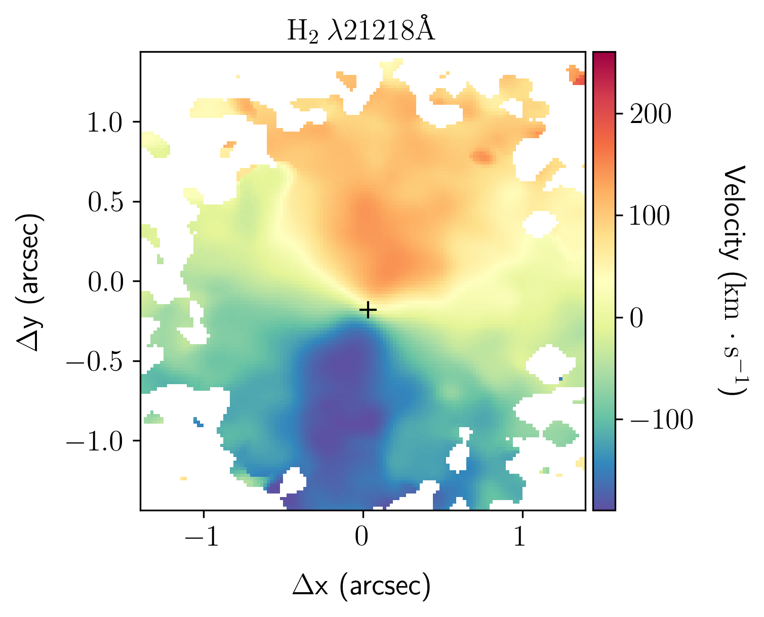
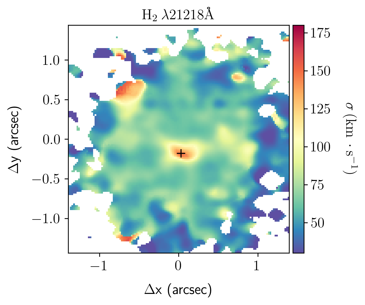
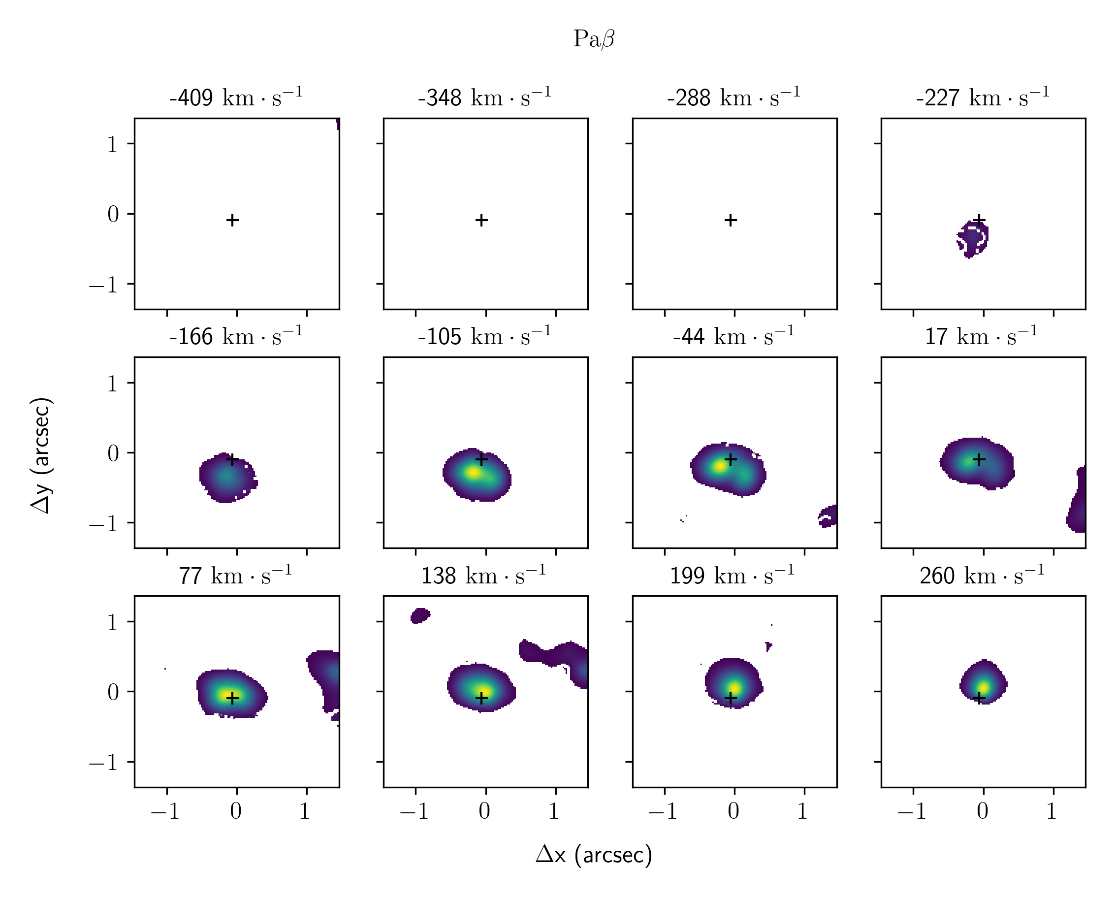
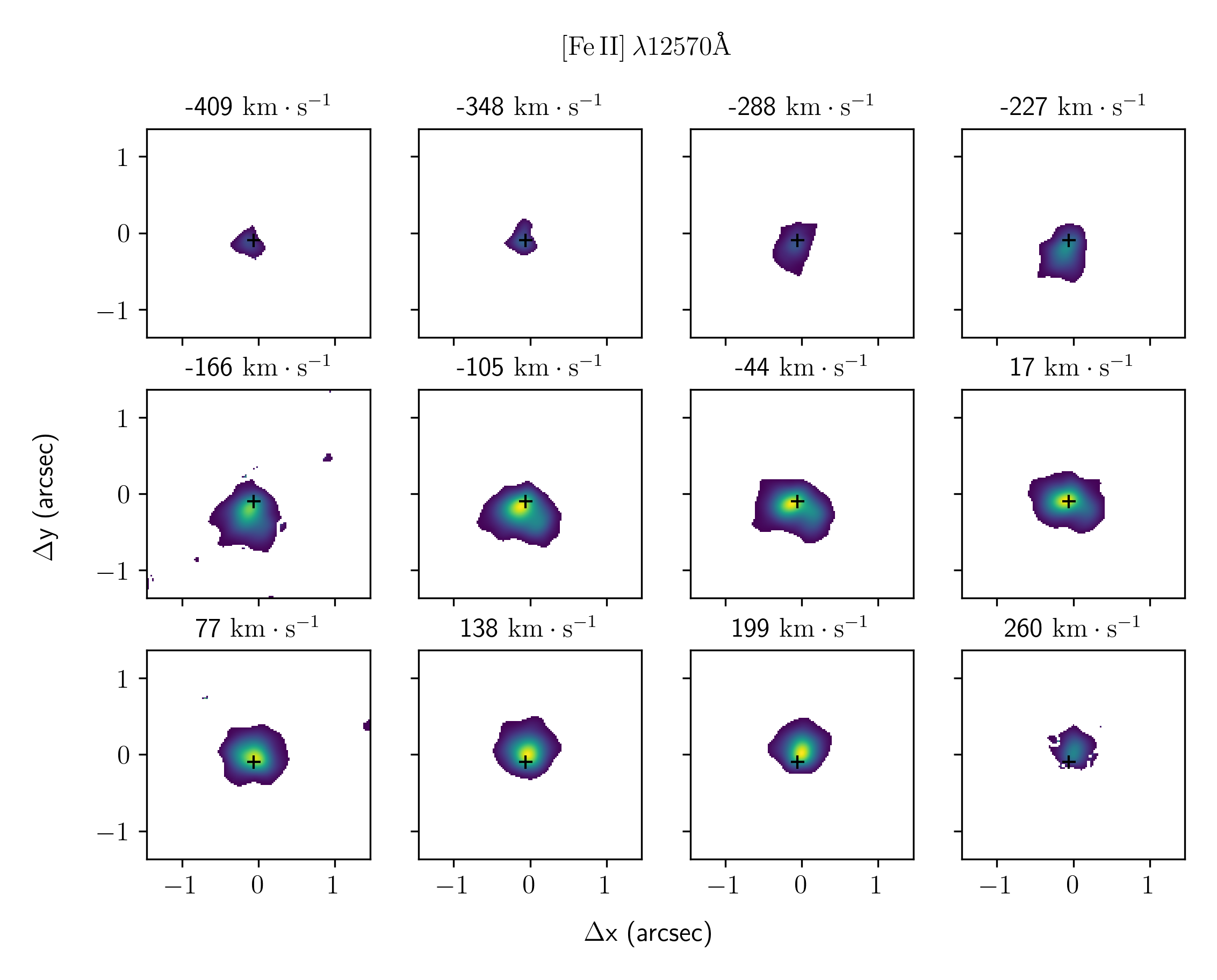
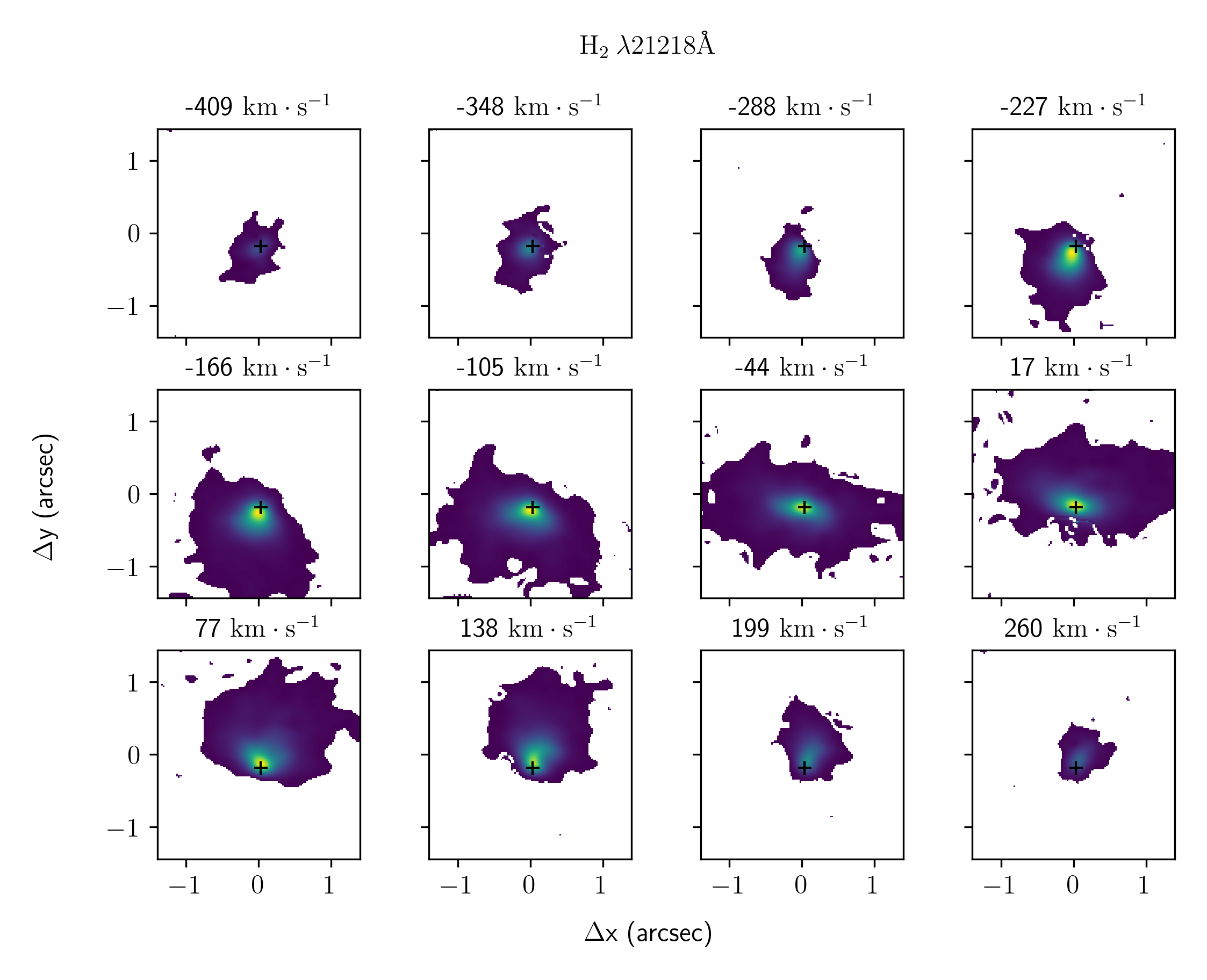
We show maps of flux distribution, radial velocities and in the first, second and third columns, respectively, of Fig. 4 for the , Å and emission lines as well as for the Å and Å narrow components. In all cases, velocities are relative to the corrected systemic velocity of the galaxy (see Sec. 5.1), and maps of velocity dispersions were corrected for the instrumental broadening. In all panels north is up, east is to the left, the black cross indicates the nucleus of the galaxy, and pixels in white were not considered in the fit. In Fig. 5 we show the flux distribution of the Å and Å broad, blue-shifted emission. The flux map of the Å emission line is shown in Fig. 6.
Hereafter, we refer to the Å , Å and Å emission lines simply as , and , respectively.
4.1 Flux distribution of the emission lines
The , , and emission features, as well as the Å molecular line show spatially resolved emission. The most compact flux distribution is found for which extends to roughly 0.4 from the nucleus of the galaxy, while the Å emission line extends over almost the entire NIFS FoV. In the J band, both the and flux distributions peak close to the galaxy nucleus and display a slight elongation in the northwest-southeast direction. In the K band, H2 emission peaks at the nucleus and smoothly decreases towards the edges of the FoV.
The and flux maps show that the flux distribution is asymmetric and that the peak is off-centred – and fluxes peak northwest, of the nucleus, and decrease towards the south-east. This may indicate either the presence of a gradient in the amount of visual extinction at the galaxy or that these lines are tracing a circumnuclear structure. We note that extended emission is also seen along the right edge of the FoV.
The flux distributions of the broad, blue-shifted components associated with the and Å emission lines are shown in the left and right panels of Fig. 5, respectively. We masked the spaxels where their peaks are smaller than three times the standard deviation of the adjacent continuum. These maps show that the main contribution of these broad, blue-shifted components to the observed emission is restricted to a compact region of radius close to the nucleus of the galaxy, and with slightly higher values towards the south-east.
Finally, the emission (Fig. 6) is overall much weaker than that of , although, same magnitude – of the order of – flux levels can be seen along a patchy distribution close to the galaxy nucleus. As a matter of fact, on average, the ratio is , reaching up to 0.3 in some locations. We have not found any report in the literature on the detection of Å emission in NGC 34. However, emission at Å has been found in other AGN in a spectroscopic survey carried out by Lamperti et al. (2017).
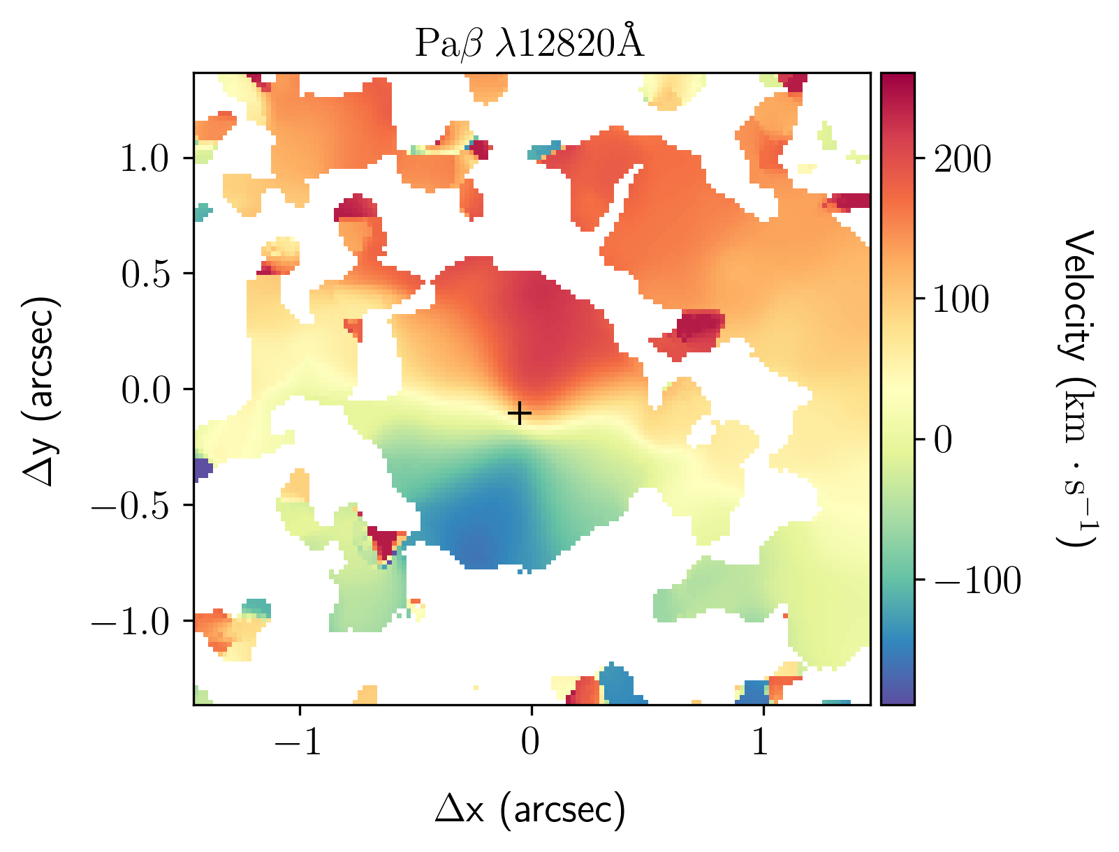
4.2 Gas kinematics
The velocity maps for all the fitted emission lines consistently show a rotation signature with a kinematic major axis at the approximate PA of , with red-shifted velocities north of the galaxy nucleus, and blue-shifted velocities to the south. For the ionized hydrogen, velocities range from to 240 . The ionized gas ( and ) shows velocities between and 170 , while the molecular hydrogen has velocities between and 140 . We could not constrain the kinematics of the emission feature due to its patchy distribution.
Velocity dispersions peak close to the nucleus of the galaxy in all cases. The highest values, 160–185 , are found for the ionized gas. Both the ionized and molecular hydrogen show maximum velocity dispersions in the range 125–145 .
We recall that we included broad, blue-shifted components to the fitting of the and Å emission lines, since fitting them with a single Gaussian could not account for the presence of broad, blue wings in a compact region close to the nucleus of the galaxy. These components have fixed radial velocities at and , and fixed velocity dispersions of 350 and 215 for the and Å emission lines, respectively.
We can further investigate the gas kinematics using channel maps, which is the mapping of the emission lines in constant velocity, or equivalently, wavelength bins. We built channel maps of the , and Å emission lines using the channel_maps module of the ifscube package. This module evaluates the adjacent continuum level and masks spaxels with flux values that after the continuum subtraction fall below a lower threshold defined by the user. Our channel maps are shown in Figs. 7–9. Maps were built between and 290 , with integrated fluxes in velocity bins of 61 centred at the velocity shown at the top of each panel. We masked spaxels with fluxes lower than 1.0 and 0.1 for the J and K bands, respectively.
All the channel maps confirm the transition from southern, blue-shifted to northern, red-shifted velocities. The rotation signature can be seen starting at the velocity channel. The channel maps of (Fig. 7) confirm the asymmetric flux distribution. We can see that lower flux values can be found south of the nucleus, and that as one moves towards red-shifted velocities, higher fluxes do not coincide with the nucleus of the galaxy, but instead, the flux distribution seems to encircle it and reaches maximum values to the north. The maps between the 17 and 138 velocity channels also show the extended emission seen at the right edge of the FoV in the flux map shown in Fig 4 (top-left).
The and Å channel maps (Figs. 8 and 9) show that for these emission lines, fluxes peak very close to the nucleus of the galaxy. More importantly, these maps confirm the presence of the broad, blue-shifted components starting at the velocity channel. For the , this blue wing is very compact and located in the nucleus of the galaxy, while for the Å it is slightly elongated to the south.
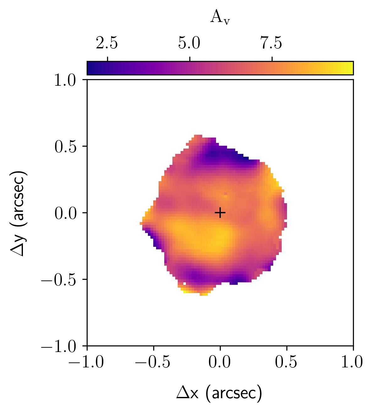
4.3 Reddening
To estimate the visual extinction throughout the inner of NGC 34, we followed Dametto et al. (2014) who adopted the ratio of total to selective extinction as from Calzetti et al. (2000), which has been shown to be the most suitable one when dealing with extinction in starbursts (Calzetti et al., 2000; Fischera et al., 2003). In the case B recombination for hydrogen (low-density limit, , Osterbrock & Ferland 2006), the intrinsic value of the emission line ratio is 5.88, and the visual extinction is:
| (1) |
The distribution throughout NGC 34 is shown in Fig. 10. The derived values range from 1.9–9.0 mag. Higher extinction can be found towards the south of the galaxy. The mean in the northern region is 6.780.86 and the median is 7.01, while in the south, the mean is 7.740.95 and the median is 7.94. These results are in full agreement with long-slit studies (see table 4 of Dametto et al., 2014).
Alonso-Herrero et al. (2006) used HST NICMOS (Near Infrared Camera and Multi-Object Spectrometer) observations to study the NIR and star-forming properties of a sample of local LIRGs. They derived extinctions in the range 2–6 mag to the stars (photometric extinctions), while extinctions to the gas, derived from the and ratios, tend to be higher, ranging from 0.5 up to 15 mag. The values found for NGC 34 indicate that its inner regions are embedded in a heavily obscured environment, which could potentially affect optical studies of high spatial resolution aiming at investigating the nature of its nuclear activity.
4.4 Emission-line ratios
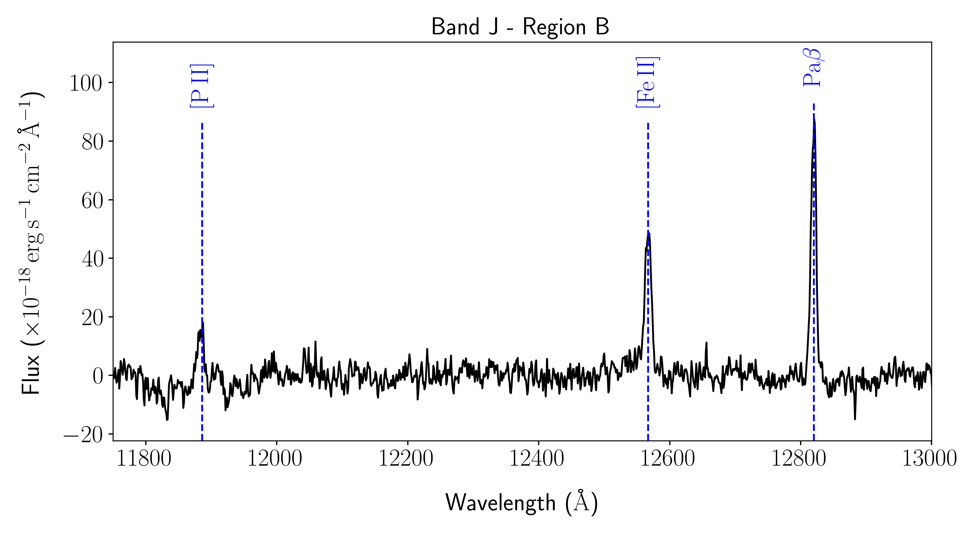
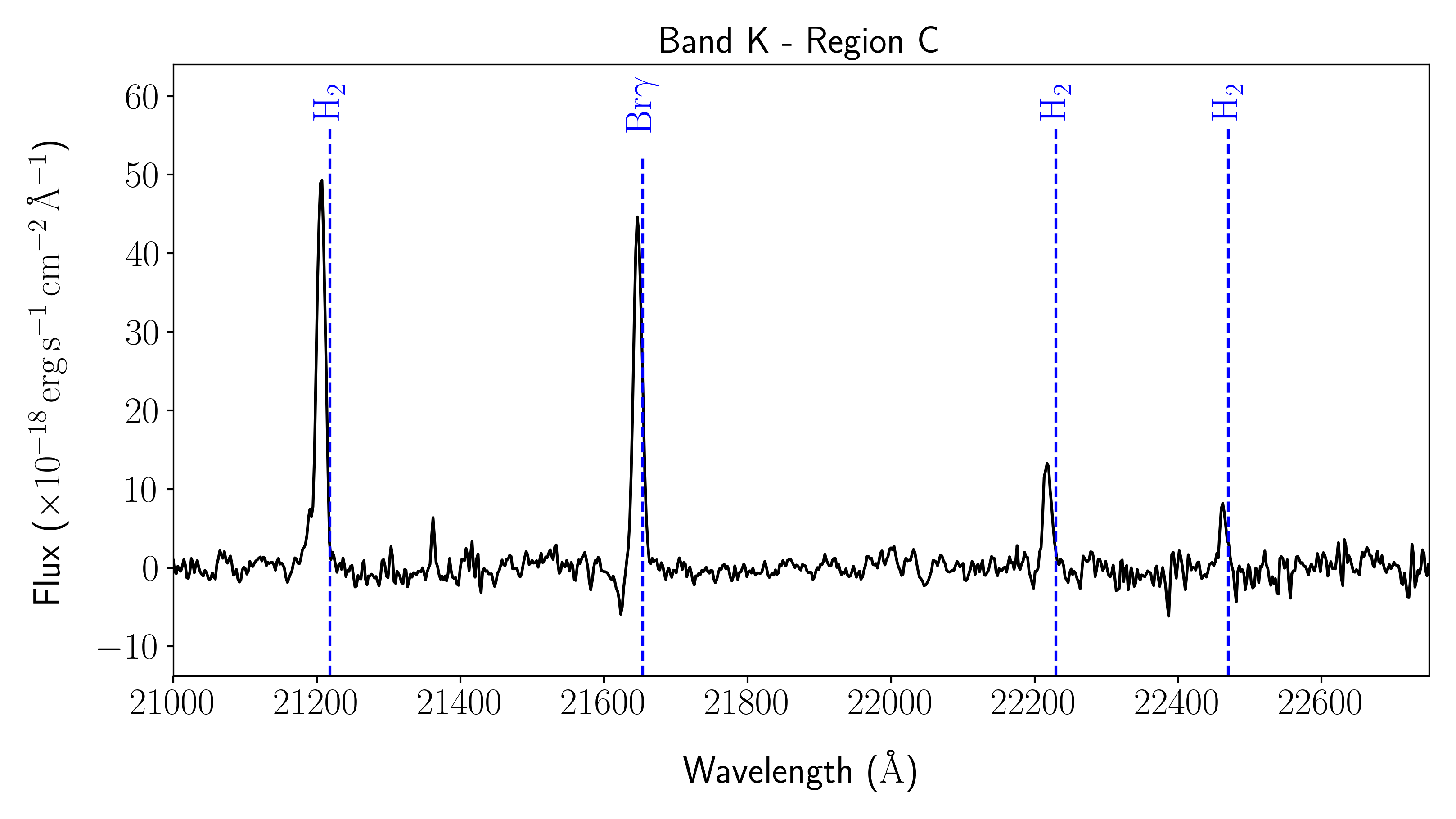
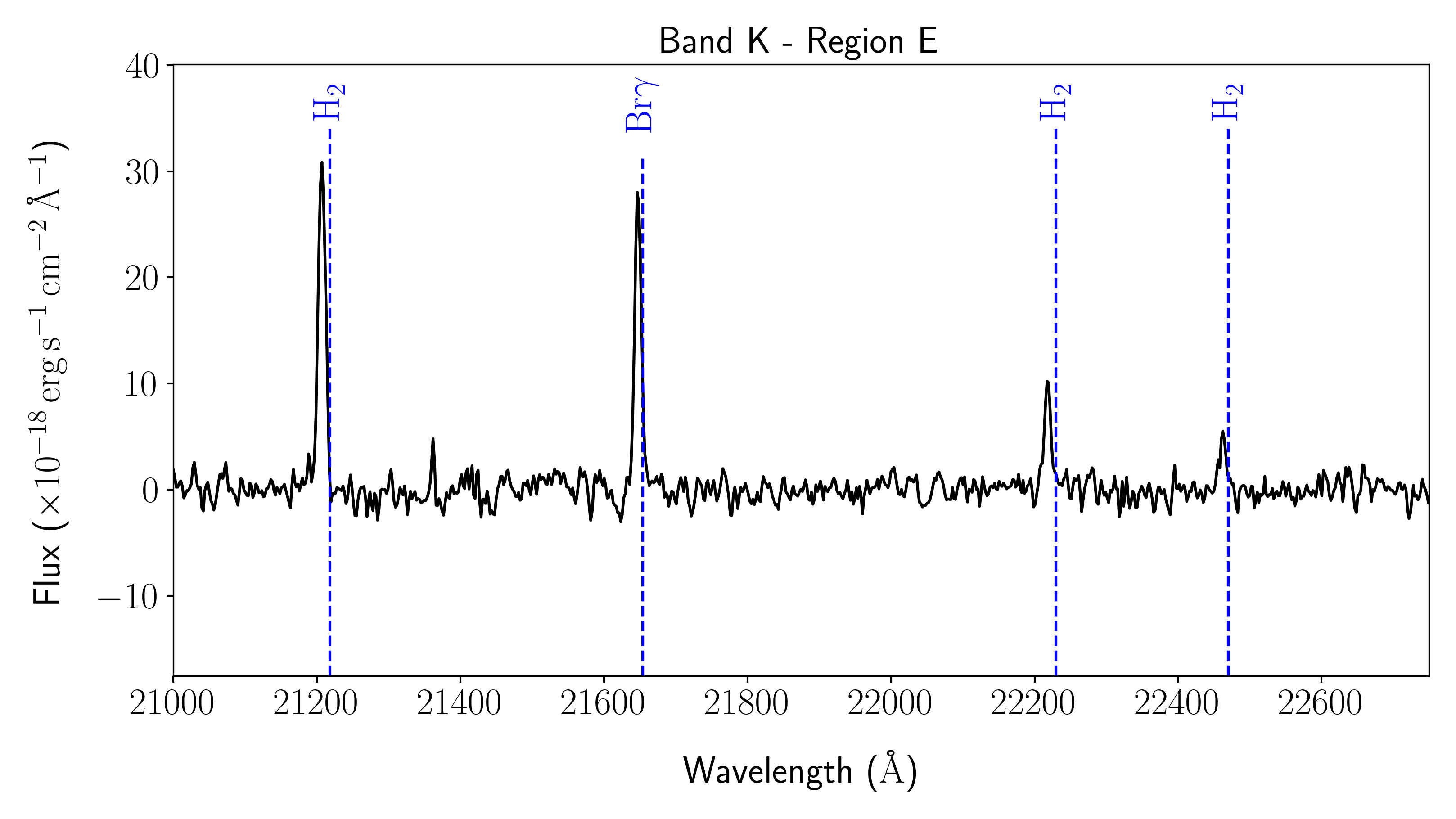
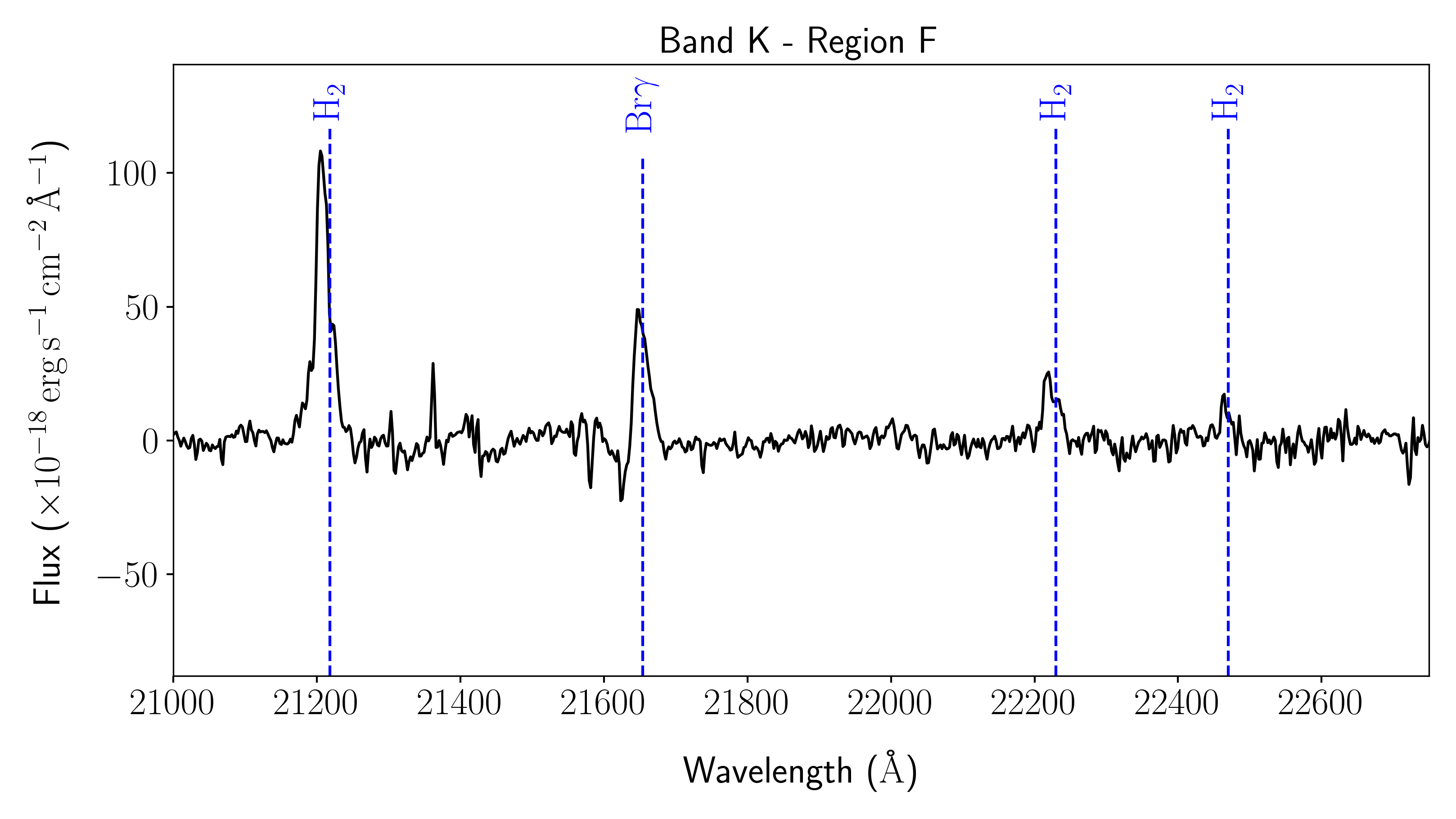
We show maps of the (top panel) and (bottom panel) emission-line ratios in Fig. 11 along with the locations of regions identified from A–F that correspond to apertures of 0.20.2. We integrated the gas spectra in each aperture and fitted the emission lines using Gaussian functions and the package ifscube, thus obtaining their amplitudes, and respective uncertainties, which were then used to estimate the uncertainties of the integrated fluxes through error propagation. Fluxes of the emission lines in each region are presented in Table 1 and the integrated spectra are shown in Appendix A.
The and line-ratios are reddening insensitive and are used to build BPT-like diagrams in the NIR (Larkin et al., 1998; Rodríguez-Ardila et al., 2004; Rodríguez-Ardila et al., 2005; Riffel et al., 2013; Colina et al., 2015; Riffel et al., 2021). The hydrogen recombination lines are tracers of UV-ionizing radiation from young OB-stars or from the AGN. The traces shocked, partially ionized regions and photo-dissociation regions, while the Å traces the hot molecular gas (TK). Star-forming galaxies (SFGs) have and , AGN-dominated systems have and , and LINERs have and (e.g.: Riffel et al. 2013).
Our maps of and for NGC 34 clearly show a ring-like structure with lower values of the ratios around the nucleus of the galaxy. Many locations in the map are consistent with pure star-formation. Along the ring-shaped structure, values range from 0.4–0.75 and reach values of 1.0 close to the nucleus of the galaxy in region F. In the case of the , the obtained values for the emission-line ratios are all consistent with the presence of an AGN, including locations along the ring-shaped structure where values range from 0.7–1.4 and reach up to 2.5 in the nucleus.
Overall, the fact that the structure in the shape of a ring around the nucleus of the galaxy can be seen in both maps of emission-line ratios, in addition to many locations displaying values consistent with pure star-formation indicate that the NGC 34 nuclear starburst is distributed in a circumnuclear star-formation ring. However, larger values found for both line ratios, especially in the case of the , indicate that additional mechanisms are required to explain the emission and the excitation of the H2 molecule, as will be discussed in section 5.3.
| Region | |||||||
|---|---|---|---|---|---|---|---|
| ( 11886Å ) | ( 12570Å ) | ( 12818Å ) | ( 21218Å ) | ( 22230Å ) | ( 22470Å ) | ( 21654Å ) | |
| A | 0.560.00 | 1.240.07 | 2.150.09 | 1.030.11 | 0.260.02 | 0.160.01 | 1.090.06 |
| B | 0.270.02 | 0.560.03 | 0.860.03 | 0.550.04 | 0.180.01 | 0.080.00 | 0.400.02 |
| C | 0.240.01 | 0.610.03 | 1.070.04 | 0.630.03 | 0.180.01 | 0.100.00 | 0.630.02 |
| D | 0.110.01 | 0.270.01 | 0.500.01 | 0.390.03 | 0.130.01 | 0.050.00 | 0.230.01 |
| E | 0.140.01 | 0.430.02 | 0.700.02 | 0.370.02 | 0.110.01 | 0.060.00 | 0.310.01 |
| F | 0.820.02 | 1.810.13 | 1.980.08 | 2.250.43 | 0.550.09 | 0.220.03 | 1.080.05 |
4.5 Principal Component Analysis Tomography
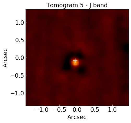
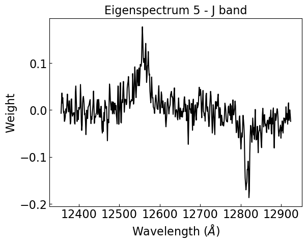
We also analysed the data cubes of NGC 34 using Principal Component Analysis (PCA) Tomography (Steiner et al., 2009). This technique uses PCA applied to data cubes in order to extract useful information from a given object (see e.g. Ricci et al. 2011, 2014, 2015; Dahmer-Hahn et al. 2019). It searches for correlations between m spectral pixels across n spaxels. A set of m eigenvectors is built as a combination of the m spectral pixels and they are ordered by their contribution of the variance (obtained with the respective eigenvalues) of the data cube. The tomograms correspond to the projection of the eigenvectors on the data cubes. In practice, the eigenvectors, also called eigenspectra, show the correlations between the wavelengths, while the tomograms reveal where such correlations occur in the spatial dimension.
We applied PCA Tomography in both J and K bands data cubes after the subtraction of the stellar component of NGC 34. In the case of the K band data cube, we used the spectral range 20814–22568 Å, which contains all H2 and the Br lines. For the J band data cube, a spectral range of 12356–12923 Å was used, containing both and Pa lines. The most relevant results revealed by the PCA Tomography correspond to the fourth eigenspectrum of the K band data cube and the fifth eigenspectrum of the J band data cube, shown in Fig. 12. Eigenspectrum 4 of the K band data cube explains 1.76 per cent of the variance and is characterised by an anti-correlation between the Br and the H21218Å lines. Its tomogram reveals a nuclear object, which is related to the H21218Å line, and a circumnuclear structure, which corresponds to the Br line. A similar scheme is seen in the fifth tomogram of the J band data cube. In this case, the eigenspectrum 5 explains 1.21 per cent of the variance and is characterised by a broad component anti-correlated with the Pa line. The nuclear object seen in tomogram 5 is related to the broad component, while the circumnuclear structure is associated with the Pa emission.
5 Discussion
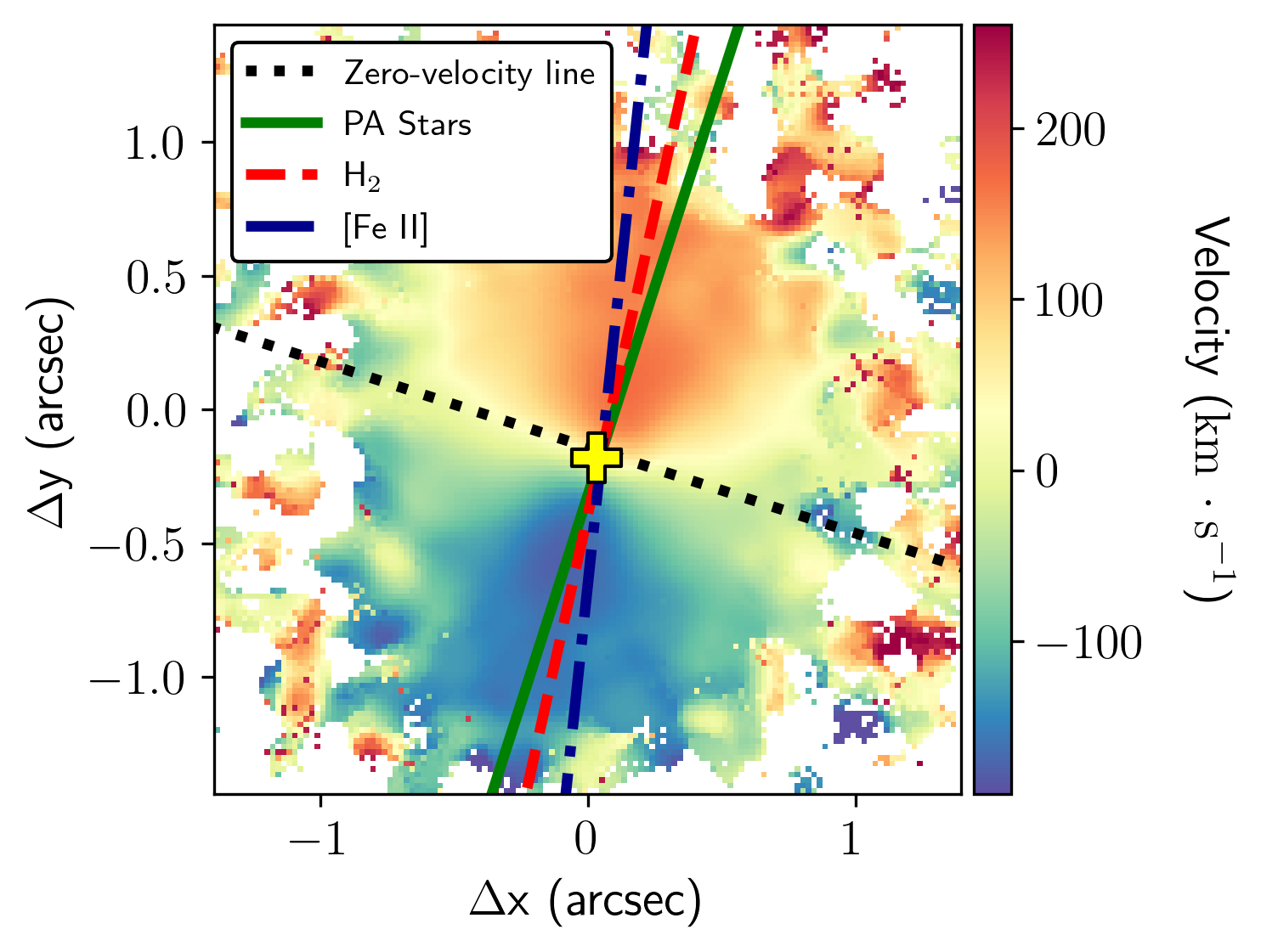
5.1 Nuclear disc of ionized and molecular gas
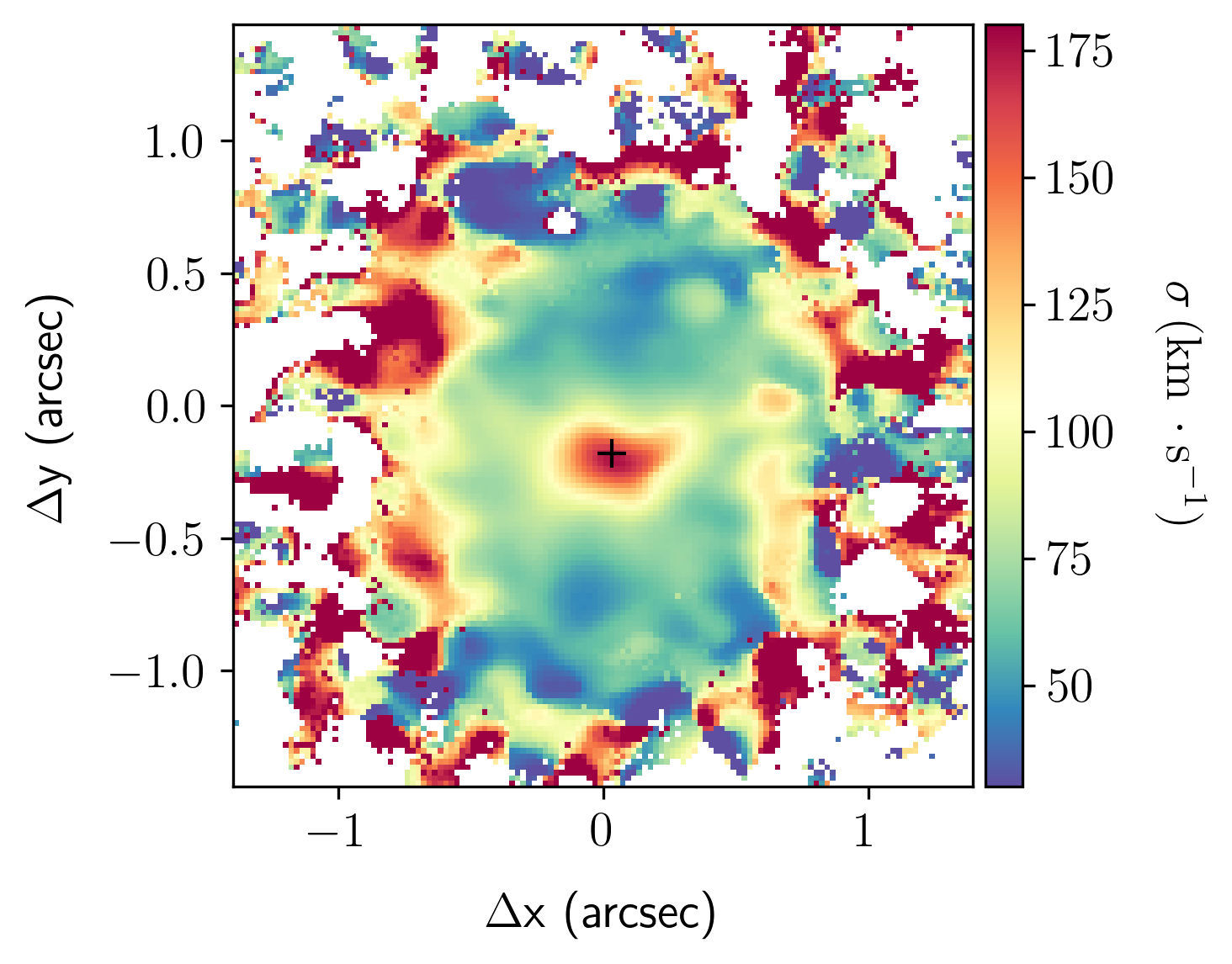
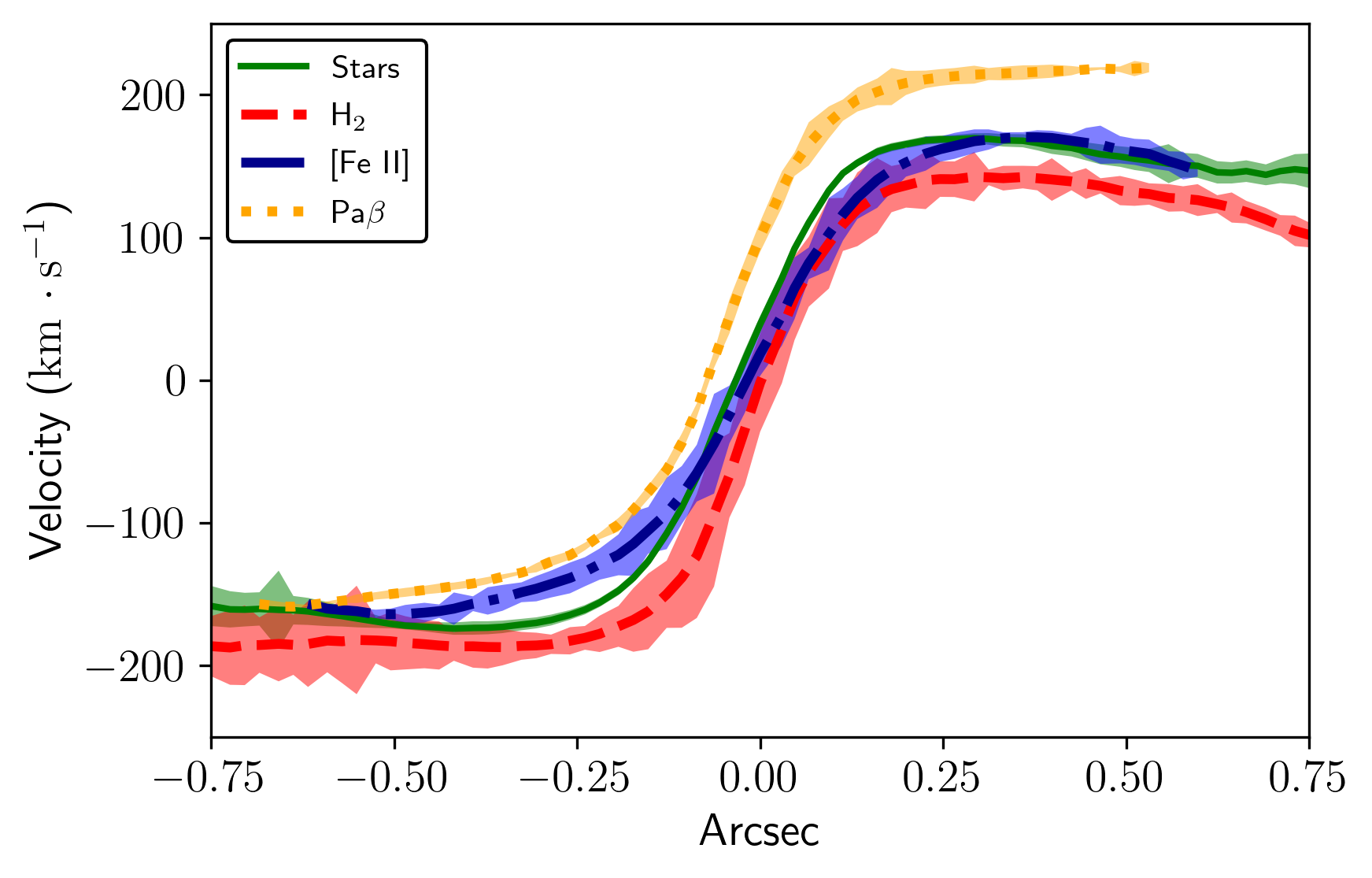
The maps of radial velocities of the fitted emission lines presented in Sec. 4.2 clearly show signature of rotation in the ionized and molecular gas phases. In order to compare the kinematics of the gas in NGC 34 with that of the stars, we carried out a new spectral synthesis in the K band data cube using the code ppxf and the Gemini library of late spectral templates (Winge et al., 2009), which was especially designed to support stellar kinematics studies in external galaxies. We also followed the recommendations of Cappellari (2017) to include only additive polynomials when using ppxf to fit the stellar kinematics. We then used the code pafit111Available at https://pypi.org/project/pafit/, which implements the method presented in Appendix C of Krajnović et al. (2006), to determine: (1) a correction () to be applied to the adopted systemic velocity of the galaxy determined from the stellar velocity field () and (2) the global kinematic PA of the stellar and gas discs.
The NGC 34 stellar velocity field is shown in the left panel of Fig. 13 and the correction to the systemic velocity is -40 , resulting in . In general, one can see that the range of velocities as well as the PA of the rotation signature of the stars are very similar to the ones found for the ionized and molecular gas, indicating that they are under the influence of the same gravitational potential. This can be straightforwardly associated with the presence of a nuclear disc (ND) of stars and gas. For the stars, the kinematic PA of the disc is . The global kinematic PAs of the ionized and molecular gas discs are and , respectively, resulting in a mean PA of . The PA of the stellar, ionized and molecular gas discs are indicated in Fig. 13 by the solid green, blue dashdot and dashed red lines, respectively. The field of stellar velocity dispersion (middle panel) show higher values in the galaxy nucleus. In the right panel of Fig. 13, we show stellar and gas velocity profiles taken along the kinematic PA of the stellar disc. Velocities rise steeply and reach maximum values in a radius smaller than 0.5 (200 pc) from the nucleus of the galaxy, indicating that the disc is compact.
Our results are in agreement with previous works presented by Fernández et al. (2014) and Xu et al. (2014), thus confirming the presence of a ND of ionized and molecular gas in NGC 34 with a northern receding and a southern approaching side. However, Xu et al. (2014) point out that the 2 kpc CO(1-0) disc found by Fernández et al. (2014) is associated with diffuse gas emission, while the much more compact 200 pc CO(6-5) disc detected by them (see Fig 1 in Xu et al. 2014) has the same distribution of the nuclear starburst traced by radio continuum emission. The kinematic PA of the CO(6-5) disc is and the rotation velocity also rises up to a radius of 0.5 and then flattens, indicating that our NIR IFU data and the ALMA observations of Xu et al. (2014) share the same kinematics.
5.2 Resolved NIR diagnostic diagram and the NGC 34 power source
As previously mentioned, the nature of the NGC 34 nuclear emission line spectrum is still under debate, with different works classifying it as due to a starburst (Mulchaey et al., 1996; Riffel et al., 2006) and/or AGN (Yuan et al., 2010; Brightman & Nandra, 2011b). In this work, we characterise the nuclear activity in NGC 34 by means of high spatial resolution observations of NIR emission lines, namely the , , and Å emission features, which are more suited for probing the dust-embedded environments typically found in (U)LIRGs. While the and emissions are mainly due to the UV-ionizing flux produced by young OB-stars (ages 10 Myr) or by the AGN, emissions by the and H2 species have different origin.
Excitation of the H2 molecule can be due to: (1) UV pumping (fluorescence), also regarded as non-thermal emission, where H2 molecules are electronically excited by the absorption of UV photons in the Lyman-Werner band (918–1108Å ) in photo-dissociation regions (PDRs), followed by rapid transitions to ro-vibrational excited levels of the ground state (e.g. Black & van Dishoeck 1987); and the thermal processes either through (2) direct heating of the molecular gas by shocks (e.g. Hollenbach & McKee 1989) or by (3) X-rays, for example, produced by an AGN (e.g. Maloney et al. 1996). Early works have already shown that for a single object, the observed H2 spectrum is often the result of multiple excitation mechanisms that are at play (e.g Mouri 1994). Similarly, emission can also be traced to shock dominated regions, associated either with radio jets, nuclear outflows and/or supernova remnants (SNRs), or to photo-ionization by a central X-ray source (AGN, Mouri et al. 2000).
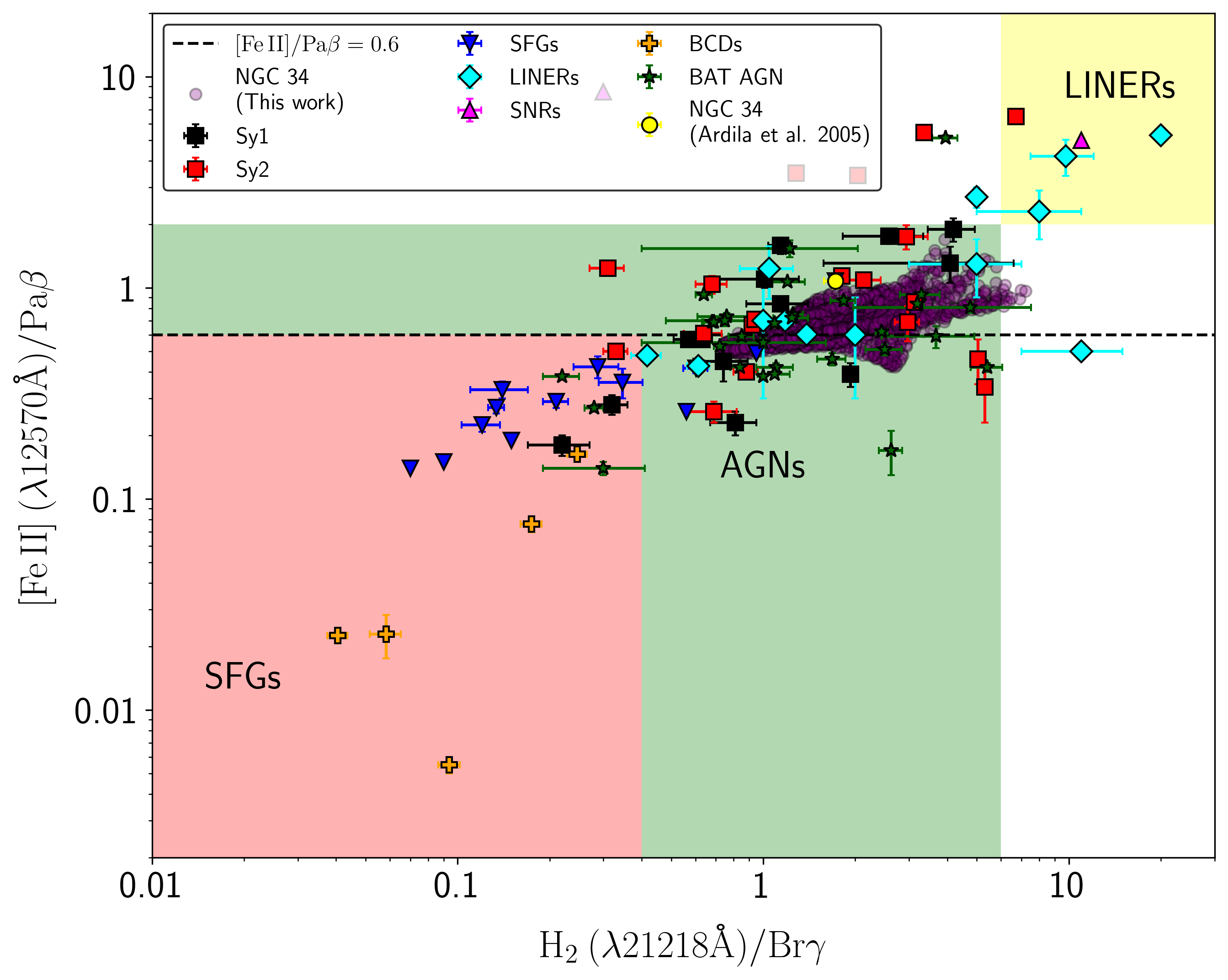
In this sense, NIR diagnostic diagrams based on the and line-ratios provide a progression in the observed values from pure photo-ionized (such as in H ii regions) to pure shock excited regions (for example, shocks in SNRs), with star-forming (SF) regions displaying low values for both ratios, while regions dominated by the AGN have intermediate values (Larkin et al., 1998; Rodríguez-Ardila et al., 2004; Rodríguez-Ardila et al., 2005; Riffel et al., 2013; Colina et al., 2015; Riffel et al., 2021).
In Fig. 14, the left panel shows our spatially resolved NIR diagnostic diagram of NGC 34 along with data collected from the literature for other sources (see Appendix B for the complete list of sources, values of the data points and references). The limiting ratio from Riffel et al. (2013) for SFGs is indicated by the horizontal, black, dashed line. A zoomed version of the diagram is presented in the right panel along with the values of line-ratios obtained in the integrated regions shown in Fig. 11 and listed in Table 1. We also included the linear relations between the and line ratios defined by Colina et al. (2015), who investigated the two-dimensional excitation structure of the interstellar medium in a sample of low-z LIRGs and Seyferts, using NIR integral field spectroscopy222Note that the linear relations presented by Colina et al. (2015) are defined on the basis of the ratio. Assuming the theoretical ratio and case B recombination, we can calculate the line ratio using (see Sec. 2.2 of Colina et al. 2015).. In their work (see Sec. 4.1 of Colina et al. 2015), distinct, linear relations in the – plane were defined for regions identified as (1) young star-forming regions (SF-young, ages 6 Myr); (2) aged, supernovae dominated regions (SNe-dominated, ages 8–40 Myr); (3) compact regions associated with nuclear AGNs (AGN-compact) and (4) diffuse, extended emitting regions where the AGN radiation field is still detected (AGN-diffuse).
Following the diagnostics presented by Riffel et al. (2013), our results indicate that all the NGC 34 spaxels fall in the AGN dominated region. However, one should note that considering only the line ratio, some spaxels fall bellow the 0.6 limiting value for SFGs. This is better illustrated by the integrated measurements taken in the regions A–F (right panel of Fig. 14). Recall that a clear ring-shaped structure around the nucleus of the galaxy can be seen in the maps of the and line ratios shown in Fig. 11. Regions A–E are all located on this circumnuclear ring. In Fig. 14, regions A, C and D are below the curve, while regions B and E are slightly above it, although considering the measured uncertainties, they could also be below this line. Region F, which is surrounded by the ring structure, is well separated from the other points in the NIR diagnostic diagram and occupies a portion of the diagram where both the and Å emission lines are enhanced. Our interpretation of these findings is that the low values found in regions A–E are due to a combination of excitation mainly caused by the stars with some contribution of the AGN, and that the nuclear starburst in NGC 34 is currently distributed in the circumnuclear star-forming ring (CNSFR) traced by these regions. The higher ratio found in region F reveals the presence of the AGN. Results presented by Rodríguez-Ardila et al. (2005) had already placed NGC 34 in the AGN dominated region of the diagram (yellow circle in Fig. 14). However, since these results were based on one-dimensional spectra, they could not isolate the CNSFR. In addition, when considering the results found by Colina et al. (2015), we can see that region F, which we associate with the AGN, does follow the linear relation defined for AGN-dominated regions. The other regions in the galaxy follow the linear relation found for regions where the radiation field of the AGN acts as a contributor to the observed emission.
Our interpretation is corroborated by the results of the PCA Tomography presented in Sec. 4.5, which clearly identify two distinct structures in the central region of NGC 34: a nuclear component which is related to the and Å emission lines; and a circumnuclear structure associated with the and emission.

5.3 The nature of the and Å emission lines
As can be seen by the NIR diagnostic diagram in Fig. 14, emission by and H2 is detected in objects displaying several degrees of nuclear activity. In starburst galaxies, emission is enhanced by supernova-driven shocks. For this reason, as the starburst ages, the level of is expected to rise due to the increasing SN activity, while the levels of the hydrogen recombination lines decrease following the aging of the stellar population. In Seyfert objects, the X-ray emission produced by the central engine is able to penetrate deeper in the molecular clouds, thus creating extensive partially ionized zones where both and H2 emissions are enhanced. Moreover, shocks associated with nuclear outflows also contribute as an additional excitation mechanism (Mouri et al., 2000).
Larkin et al. (1998) point out that while H2 can be easily destroyed, 98 per cent of the iron is tied up in dust grains. Therefore, in order to invoke a single mechanism to power both lines, it must not destroy the H2 molecules and must free up iron through dust grain destruction, both of which can be achieved in partially ionized zones created by the nuclear X-ray emission.
The centre of NGC 34 hosts a hard X-ray source associated with an obscured Seyfert 2 nucleus (Esquej et al., 2012). The fact that region F not only shows higher and values but also clearly lies in a different position in the NIR diagnostic diagram in Fig.14 can be explained by an enhancement of and H2 due to the AGN X-ray emission. Moreover, although contribution from the ionizing flux related to the circumnuclear stellar activity likely plays a role in powering both the and H2 emissions in the locations where the values are low, an additional mechanism is necessary mainly to explain the enhanced H2 emission in these same locations. Such an additional excitation component could also be due to the X-rays emitted by the central engine.
Following Riffel et al. (2008a) and Zuther et al. (2007), we can use the models of Maloney et al. (1996) to verify if X-ray heating by a source with intrinsic luminosity is a viable H2 excitation mechanism. Considering a cloud at a distance from a hard X-ray source and with gas density , the emergent Å flux can be obtained from figure 6 in Maloney et al. (1996) through the determination of the effective ionization parameter :
| (2) |
where is the incident X-ray flux at the distance , is total hydrogen gas density in units of 105 cm-3 and is the attenuating column density between the AGN and the gas cloud in units of 1022 cm-2. The value of can be determined using . We calculated for three different distances from the AGN (40, 80 and 120 pc) adopting the intrinsic hard X-ray luminosity (Esquej et al., 2012), (Fernández et al., 2014) and for a gas density333The models of Maloney et al. (1996) of X-ray irradiated molecular gas were calculated for and cm-3. However, the former does not provide predictions on the observed H2 fluxes in every region of interest of the source. Therefore, for completeness, we chose to perform our calculations. of cm-3. With the aid of figure 6(a) in Maloney et al. (1996), we determined the emergent H2 flux in for an aperture of (the dimensions of a spaxel in our datacubes), which corresponds to a solid angle of 1.03 10-14 sr. Our results are shown in Table 2. The observed Å fluxes were determined from three different apertures centred in region F as follows: (1) at pc, log(F) corresponds to the mean flux value in a spaxel located in a circular aperture of radius 40 pc, (2) at pc, log(F) corresponds to the mean flux value in a spaxel located in a ring with inner and outer radii of 60 and 100 pc, respectively, and (3) at pc, log(F) corresponds to the mean flux value in a spaxel located in a ring with inner and outer radii of 100 and 140 pc, respectively.
Our estimates indicate that X-ray heating can fully account for the H2 emission seen in region F, which is probably associated with the AGN. For larger distances, although X-rays contribute with some amount to the observed Å fluxes, they are not the dominant excitation mechanism. Therefore we conclude that, in NGC 34, the observed and H2 emissions are due to a combination of photo-ionization by young stars, excitation by X-rays produced by the AGN and shocks. Mingozzi et al. (2018), when modelling the CO spectral line energy distribution, did not find that shocks contribute significantly to the heating of the molecular gas in NGC 34. However, our results provide kinematic signatures of shocks, as evidenced by the broad and H2 components, indicating that shocks do contribute to the observed emission.
Note that our calculations using equation 2 were carried out assuming a column density derived from radio observations of the atomic hydrogen (H i at 21 cm, Fernández et al. 2014). The column densities obtained by Esquej et al. (2012) from X-rays and by Xu et al. (2014) using ALMA CO(6-5) observations are of the order . In this case, the predicted H2 intensities at pc would be two orders of magnitude lower than the ones shown in Table 2, indicating that even at the nucleus of NGC 34, the AGN would have a minor role in the observed H2 emission. This is unlikely considering the discussion presented in Sec. 5.2. Rodríguez-Ardila et al. (2004) also estimated the H2 fluxes for a list of sources using the models of Maloney et al. (1996) and found that the calculations using derived from X-rays result in a poorer fit compared to the calculations using derived from radio observations. They concluded that this is because derived from X-rays probes obscuring material in the innermost regions of active galaxies, while H2 and also emissions must arise farther out in the narrow line region, thus justifying the adoption of a column density obtained from 21 cm observations.
We further investigate the nature of the H2 emission using the ratio between the Å and Å emission lines to distinguish thermal () from non-thermal () excitation mechanisms of the H2 molecule (Mouri, 1994). In NGC 34, in all regions, thus confirming that the K-band H2 lines are predominantly excited by thermal processes (shocks and/or X-ray heating). We can not, however, rule out the contribution of UV-fluorescence to the observed H2 spectrum since the H2 emission at 21218Å is itself much more sensitive to thermal processes than the Å line, which is a tracer of fluorescence (Black & van Dishoeck, 1987).
The predominance of thermal processes in the excitation of the H2 molecule is further illustrated by the fact that a broad, blue-shifted component is only detected in the H2 emission at 21218Å . The velocity and line width of this blue wing, as well as of that seen in , indicate that the central regions of NGC 34 also drive a nuclear outflow of molecular and ionized gas. Although the outflow could, in principle, be driven either by the AGN, by winds associated with the circumnuclear starburst or by SN-driven shocks, we favour the first one since (1) the highest fluxes of these broad components coincide, or almost coincide, with the nucleus of the galaxy and (2) we do not observe the high values expected according to the linear relation defined by Colina et al. (2015) for SNe-dominated regions, where SN-driven shocks are responsible for enhancing the emission. In the analysis carried out by Colina et al. (2015) for the composite LIRG NGC 5135 for example, they found a value larger than 1.5 for the ratio at the location of peak associated with a SNe-dominated circumnuclear star-forming clump. Therefore, we conclude that in NGC 34, an AGN-driven nuclear outflow is the most likely primary source of shock excitation of the H2 and species.
Finally, we can also estimate the H2 vibrational excitation temperature using (Reunanen et al., 2002). We find a mean value of 2504174 K, which is in the range of values found for the H2 thermal components in other sources (1800–2700 K, Reunanen et al. 2002). Rodríguez-Ardila et al. (2005) derived an upper limit of 1800 K for NGC 34. However, this result was based on one-dimensional spectra and includes contribution from the broad H2 component. If we include the contribution of the broad, blue-shifted component to the observed Å flux, we find = 2196154 K. The values found for support the assumption used in eq. 5.5 to estimate the mass of hot H2.
| Observed | ||||
|---|---|---|---|---|
| (pc) | log(F) | log | log(F) | |
| (1) | 40 | -16.7 | -1.8 | -16.2 |
| (2) | 80 | -17.0 | -2.4 | -18.7 |
| (3) | 120 | -17.2 | -2.8 | -18.5 |
5.4 Circumnuclear star formation ring
Our maps of emission line ratios and the J and K-bands PCA Tomography show that the nuclear starburst in NGC 34 is distributed in a CNSFR. We can use the luminosity () to estimate the SFR in the ring adopting the following relation (Kennicutt, 1998):
| (3) |
The integrated, extinction corrected flux in the continuous ring A–E–A, with inner and outer radii of 60 and 180 pc, respectively, is , and . From equation 3, we derive . Also based on the luminosity, Valdés et al. (2005) estimated a SFR = 26.7 , and Dametto et al. (2014) found SFR = 9.63 .
Valdés et al. (2005) carried out NIR medium-resolution spectroscopy of a sample of (U)LIRGs and found that the luminosity provides SFRs which are on average 60 per cent of those derived from the far infrared luminosity. In the case of NGC 34, they found SFR(LFIR) = 49.9 . They stated that although the AGN might contribute to the infrared emission, this contribution would have to exceed 80 per cent to explain this large discrepancy. Alonso-Herrero et al. (2006) studied the NIR and star-forming properties of a sample of local LIRGs and also reported that the SFRs derived from the number of ionizing photons are on average 0.2–0.3 dex lower than those inferred from the total IR luminosity. This is because the luminosities of hydrogen recombination lines trace the most recent SFR, and there is a tendency for the measured IR luminosity to include some contribution from older stars. In addition, Alonso-Herrero et al. (2012) performed the spectral decomposition of a complete-volume-limited sample of local LIRGs and found that for the majority of them, the total AGN bolometric contribution to the observed IR luminosities has an upper limit of 5 per cent. Therefore, most of their IR luminosities are related to star formation processes.
We point out that the SFR of NGC 34 derived by us is a lower limit since our observations provide a smaller aperture compared to previous works, and also due to the fact that the circumnuclear ring may extend to a larger radius. CNSFRs have been detected in a variety of LIRGs with diameters ranging from 0.7 to 2 kpc (e.g Alonso-Herrero et al. 2006).
5.5 Mass of ionized and molecular gas
We can estimate the mass of ionized and molecular gas in NGC 34 using integrated, extinction corrected fluxes of and Å . Following Storchi-Bergmann et al. (2009) and assuming an electron temperature of , the mass of ionized hydrogen, in solar masses, is given by:
| (4) |
where is the integrated flux, is the distance to NGC 34 and we have assumed an electron density , which is the mean value calculated by Kakkad et al. (2018) using the lines for a sample of nearby () Seyfert 1s, Seyfert 2s and AGN-Starburst composite systems.
The mass of hot H2 in solar masses can be estimated as follows (Scoville et al., 1982):
| (5) |
where, is the proton mass, is the integrated flux of the Å emission line, is the distance to the galaxy, is the Planck constant and is the frequency of the H2 line. Adopting a typical vibrational excitation temperature of , which is consistent with the values we have obtained in Sec. 5.3, the population fraction is and the transition probability is (Turner et al., 1977; Scoville et al., 1982).
We carried out the mass estimates for the inner of the galaxy, since this corresponds to the region where we have derived visual extinction values to be applied to the observed fluxes. The integrated, extinction-corrected and Å fluxes are and , respectively, resulting in and . Although M is nearly 103 times larger than , we note that the later refers only to the hot molecular gas that gives rise to the observed NIR emission lines. The value derived by us for the hot molecular gas mass is similar to the one presented by Rodríguez-Ardila et al. (2005) who found .
Following Mazzalay et al. (2013), we can also estimate the mass of cold molecular gas using:
| (6) |
where is the luminosity of the H2 line. We find for NGC 34, which is roughly six orders of magnitude higher than that derived for the hot H2. This is in agreement with previous works that estimated the mass of cold molecular gas in NGC 34 from observations of the CO molecule (, Chini et al. 1992; Kruegel et al. 1990; Kandalyan 2003).
6 Conclusions
The galaxy NGC 34 is a local LIRG whose nature of its emission line features has been explained either as due to a pure starburst or due to a starburst–AGN composite source. In this work, we used AO-assisted IFU observations carried out with the NIFS instrument in the J and K bands to map the inner of the galaxy in order to investigate the excitation mechanisms of its NIR spectrum. We summarise our main findings as follows:
-
•
The NGC 34 NIR spectra are characterised by the Å , Å , Å and emission features in the J-band, and by the Å , , Å and Å emission lines in the K-band;
-
•
We report the detection of emission at Å ;
-
•
The fluxes of all emission features but and peak at the nucleus of the galaxy. The and flux distributions are asymmetric and peak north-west. This asymmetry is confirmed by the channel maps and indicates that the hydrogen recombination lines are tracing a circumnuclear structure.
-
•
Through the analysis of the gas kinematics, we confirm the presence of a ND of ionized and molecular gas in NGC 34, with a northern-receding and a southern-approaching side. We determined that the mean kinematic PA of the gas disc is ;
-
•
We find that the NGC 34 nuclear starburst is distributed in a CNSFR with approximate inner and outer radii of 60 and 180 pc, respectively, as revealed by maps of the and emission-line ratios. These maps clearly show a ring-like structure with lower values around the nucleus of the galaxy, especially for the ratios, where many locations display values that are consistent with pure star formation (, Riffel et al. 2013). The higher values found for both ratios indicate that multiple excitation mechanisms are at play in NGC 34.
-
•
The presence of a CNSFR is corroborated by the PCA Tomography, which shows a nuclear object associated with the Å and emission lines, and a circumnuclear structure associated with the and lines.
-
•
The resolved NIR diagnostic diagram based on the and emission-line ratios show that all the NGC 34 spaxels fall in the AGN dominated region. Integrated measurements taken in different regions A–F also confirm that the inner regions of NGC 34 are characterised by a nuclear and circumnuclear structures. Regions A–E trace the CNSFR since the ratios lie bellow or slightly above the limiting value of 0.6 for pure star formation defined by Riffel et al. (2013). Region F, in the nucleus of the galaxy, clearly occupies a portion of the diagram where both the and Å lines are enhanced relative to the hydrogen recombination lines. Therefore, we associate region F with the AGN. NGC 34 hosts a hard X-ray source associated with an obscured Seyfert 2 nucleus (Esquej et al., 2012), and whose incident flux on the gas clouds could contribute to their enhancement. Moreover, the line ratios observed in region F follow the linear relation found by Colina et al. (2015) for AGN-dominated regions;
-
•
Using the models of Maloney et al. (1996), we concluded that X-ray heating can fully account for the Å emission in the nucleus of the galaxy (region F), but it is not the predominant excitation mechanism at larger distances. Therefore we state that, in NGC 34, emission by and H2 is due to a combination of photo-ionization by young stars, excitation by X-rays produced by the AGN and shocks as evidenced by the kinematic signatures of outflows in the ionized and molecular gas phases;
-
•
We detected broad, blue-shifted components associated with the and Å emission lines at and , respectively, that can be interpreted as a nuclear outflow of ionized and molecular gas. Our results indicate that the outflow is AGN-driven and is the most likely primary source of shock excitation of the H2 and species;
-
•
From the luminosity of the CNSFR we estimated a lower limit of ;
-
•
The mass of ionized hydrogen in NGC 34 is , and the mass of cold molecular gas is , in agreement with previous works.
Our results indicate that the merger remnant NGC 34 is a gas-rich system that hosts an AGN surrounded by a ring of star-formation. The AGN and the CNSFR are embedded in a compact, highly obscured environment making it difficult for optical studies to probe such inner, dusty regions. A common, evolutionary picture for (U)LIRGs is that mergers of gas-rich galaxies are responsible for funneling large amounts of molecular gas towards the centre of the merger, thus providing fuel to the starburst and AGN, both of which act on heating the surrounding dust. As the starburst declines, and the combined effects of SN explosions and AGN feedback clear out the nuclear dust, these objects become optically selected quasars (e.g. Sanders et al. 1988). In the case of NGC 34, we, therefore, conclude that we may be witnessing the early, evolutionary stage of a dust-enshrouded AGN.
Acknowledgements
JCM thanks Coordenação de Aperfeiçoamento de Pessoal de Nível Superior (CAPES) for the financial support under the grant 88882.316156/2019-01. RR and RAR thanks Conselho Nacional de Desenvolvimento Científico e Tecnológico (CNPq), CAPES and Fundação de Amparo à Pesquisa do Estado do Rio Grande do Sul (FAPERGS) for the financial support. TVR also thanks CNPq for the financial support under the grant 306790/2019-0. NZD acknowledges partial support from FONDECYT through project 3190769. We thank Dr. João Evangelista Steiner†(1950–2020) for enlightening us with comments and suggestions before embarking on his journey to the stars. The authors also thank the anonymous referee for his/her careful revision that helped us to improve the quality of this manuscript. Based on observations obtained at the international Gemini Observatory, which is managed by the Association of Universities for Research in Astronomy (AURA) under a cooperative agreement with the National Science Foundation, on behalf of the Gemini Observatory partnership: the National Science Foundation (United States), National Research Council (Canada), Agencia Nacional de Investigación y Desarrollo (Chile), Ministerio de Ciencia, Tecnología e Innovación (Argentina), Ministério da Ciência, Tecnologia, Inovações e Comunicações (Brazil), and Korea Astronomy and Space Science Institute (Republic of Korea). This research made use of observations made with the NASA/ESA Hubble Space Telescope, and obtained from the Hubble Legacy Archive, which is a collaboration between the Space Telescope Science Institute (STScI/NASA), the Space Telescope European Coordinating Facility (ST-ECF/ESAC/ESA) and the Canadian Astronomy Data Centre (CADC/NRC/CSA). This research made use of: Astropy,444http://www.astropy.org a community-developed core Python package for Astronomy (Astropy Collaboration et al., 2013; Price-Whelan et al., 2018); Photutils, an Astropy package for detection and photometry of astronomical sources (Bradley et al., 2021); the NumPy (Harris et al., 2020) and Matplotlib (Hunter, 2007) Python libraries.
Data availability
The data underlying this article are available in the Gemini Observatory Archive at https://archive.gemini.edu/searchform, and can be accessed with the Program ID GN-2011B-Q-71.
References
- Alonso-Herrero et al. (2006) Alonso-Herrero A., Rieke G. H., Rieke M. J., Colina L., Pérez-González P. G., Ryder S. D., 2006, ApJ, 650, 835
- Alonso-Herrero et al. (2012) Alonso-Herrero A., Pereira-Santaella M., Rieke G. H., Rigopoulou D., 2012, ApJ, 744, 2
- Astropy Collaboration et al. (2013) Astropy Collaboration et al., 2013, A&A, 558, A33
- Baldwin et al. (1981) Baldwin J. A., Phillips M. M., Terlevich R., 1981, PASP, 93, 5
- Black & van Dishoeck (1987) Black J. H., van Dishoeck E. F., 1987, ApJ, 322, 412
- Bradley et al. (2021) Bradley L., et al., 2021, astropy/photutils: 1.0.2, doi:10.5281/zenodo.4453725, https://doi.org/10.5281/zenodo.4453725
- Brightman & Nandra (2011a) Brightman M., Nandra K., 2011a, MNRAS, 413, 1206
- Brightman & Nandra (2011b) Brightman M., Nandra K., 2011b, MNRAS, 414, 3084
- Calzetti et al. (2000) Calzetti D., Armus L., Bohlin R. C., Kinney A. L., Koornneef J., Storchi-Bergmann T., 2000, ApJ, 533, 682
- Cappellari (2017) Cappellari M., 2017, MNRAS, 466, 798
- Chini et al. (1992) Chini R., Kruegel E., Steppe H., 1992, A&A, 255, 87
- Colina et al. (2015) Colina L., et al., 2015, A&A, 578, A48
- Cushing et al. (2005) Cushing M. C., Rayner J. T., Vacca W. D., 2005, ApJ, 623, 1115
- Dahmer-Hahn et al. (2019) Dahmer-Hahn L. G., et al., 2019, MNRAS, 489, 5653
- Dale et al. (2004) Dale D. A., et al., 2004, ApJ, 601, 813
- Dametto et al. (2014) Dametto N. Z., Riffel R., Pastoriza M. G., Rodríguez-Ardila A., Hernandez-Jimenez J. A., Carvalho E. A., 2014, MNRAS, 443, 1754
- Davies et al. (2007) Davies R. I., Müller Sánchez F., Genzel R., Tacconi L. J., Hicks E. K. S., Friedrich S., Sternberg A., 2007, ApJ, 671, 1388
- Deeley et al. (2017) Deeley S., et al., 2017, MNRAS, 467, 3934
- Esquej et al. (2012) Esquej P., Alonso-Herrero A., Pérez-García A. M., Pereira-Santaella M., Rigopoulou D., Sánchez-Portal M., Castillo M., et al., 2012, MNRAS, 423, 185
- Fernández et al. (2010) Fernández X., van Gorkom J. H., Schweizer F., Barnes J. E., 2010, AJ, 140, 1965
- Fernández et al. (2014) Fernández X., Petric A. O., Schweizer F., van Gorkom J. H., 2014, AJ, 147, 74
- Fischera et al. (2003) Fischera J., Dopita M. A., Sutherland R. S., 2003, ApJ, 599, L21
- Guainazzi et al. (2005) Guainazzi M., Matt G., Perola G. C., 2005, A&A, 444, 119
- Harris et al. (2020) Harris C. R., et al., 2020, Nature, 585, 357
- Harrison (2017) Harrison C. M., 2017, Nature Astronomy, 1, 0165
- Hollenbach & McKee (1989) Hollenbach D., McKee C. F., 1989, ApJ, 342, 306
- Hopkins et al. (2008) Hopkins P. F., Hernquist L., Cox T. J., Kereš D., 2008, ApJS, 175, 356
- Hung et al. (2014) Hung C.-L., et al., 2014, ApJ, 791, 63
- Hunter (2007) Hunter J. D., 2007, Computing in Science & Engineering, 9, 90
- Izotov & Thuan (2011) Izotov Y. I., Thuan T. X., 2011, ApJ, 734, 82
- Kakkad et al. (2018) Kakkad D., et al., 2018, A&A, 618, A6
- Kandalyan (2003) Kandalyan R. A., 2003, A&A, 398, 493
- Kawakatu & Wada (2008) Kawakatu N., Wada K., 2008, ApJ, 681, 73
- Kennicutt (1998) Kennicutt Robert C. J., 1998, ARA&A, 36, 189
- Kewley et al. (2001) Kewley L. J., Heisler C. A., Dopita M. A., Lumsden S., 2001, ApJS, 132, 37
- Kewley et al. (2006) Kewley L. J., Groves B., Kauffmann G., Heckman T., 2006, MNRAS, 372, 961
- Knop et al. (2001) Knop R. A., Armus L., Matthews K., Murphy T. W., Soifer B. T., 2001, AJ, 122, 764
- Krajnović et al. (2006) Krajnović D., Cappellari M., de Zeeuw P. T., Copin Y., 2006, MNRAS, 366, 787
- Kruegel et al. (1990) Kruegel E., Chini R., Steppe H., 1990, A&A, 229, 17
- Lamperti et al. (2017) Lamperti I., et al., 2017, MNRAS, 467, 540
- Larkin et al. (1998) Larkin J. E., Armus L., Knop R. A., Soifer B. T., Matthews K., 1998, ApJS, 114, 59
- Lonsdale et al. (2006) Lonsdale C. J., Farrah D., Smith H. E., 2006, Ultraluminous Infrared Galaxies. p. 285, doi:10.1007/3-540-30313-8_9
- Malkan et al. (1998) Malkan M. A., Gorjian V., Tam R., 1998, ApJS, 117, 25
- Maloney et al. (1996) Maloney P. R., Hollenbach D. J., Tielens A. G. G. M., 1996, ApJ, 466, 561
- Mazzalay et al. (2013) Mazzalay X., et al., 2013, MNRAS, 428, 2389
- Menezes et al. (2014) Menezes R. B., Steiner J. E., Ricci T. V., 2014, MNRAS, 438, 2597
- Mingozzi et al. (2018) Mingozzi M., et al., 2018, MNRAS, 474, 3640
- Mouri (1994) Mouri H., 1994, ApJ, 427, 777
- Mouri et al. (2000) Mouri H., Kawara K., Taniguchi Y., 2000, ApJ, 528, 186
- Mulchaey et al. (1996) Mulchaey J. S., Wilson A. S., Tsvetanov Z., 1996, ApJS, 102, 309
- Nardini et al. (2010) Nardini E., Risaliti G., Watabe Y., Salvati M., Sani E., 2010, MNRAS, 405, 2505
- Osterbrock & Ferland (2006) Osterbrock D. E., Ferland G. J., 2006, Astrophysics of gaseous nebulae and active galactic nuclei
- Pérez-Torres et al. (2021) Pérez-Torres M., Mattila S., Alonso-Herrero A., Aalto S., Efstathiou A., 2021, A&ARv, 29, 2
- Planck Collaboration et al. (2020) Planck Collaboration et al., 2020, A&A, 641, A6
- Price-Whelan et al. (2018) Price-Whelan A. M., et al., 2018, AJ, 156, 123
- Prouton et al. (2004) Prouton O. R., Bressan A., Clemens M., Franceschini A., Granato G. L., Silva L., 2004, A&A, 421, 115
- Rayner et al. (2009) Rayner J. T., Cushing M. C., Vacca W. D., 2009, ApJS, 185, 289
- Reunanen et al. (2002) Reunanen J., Kotilainen J. K., Prieto M. A., 2002, MNRAS, 331, 154
- Ricci et al. (2011) Ricci T. V., Steiner J. E., Menezes R. B., 2011, ApJ, 734, L10
- Ricci et al. (2014) Ricci T. V., Steiner J. E., Menezes R. B., 2014, MNRAS, 440, 2419
- Ricci et al. (2015) Ricci T. V., Steiner J. E., Giansante L., 2015, A&A, 576, A58
- Riffel et al. (2006) Riffel R., Rodríguez-Ardila A., Pastoriza M. G., 2006, A&A, 457, 61
- Riffel et al. (2008a) Riffel R. A., Storchi-Bergmann T., Winge C., McGregor P. J., Beck T., Schmitt H., 2008a, MNRAS, 385, 1129
- Riffel et al. (2008b) Riffel R., Pastoriza M. G., Rodríguez-Ardila A., Maraston C., 2008b, MNRAS, 388, 803
- Riffel et al. (2009) Riffel R., Pastoriza M. G., Rodríguez-Ardila A., Bonatto C., 2009, MNRAS, 400, 273
- Riffel et al. (2013) Riffel R., Rodríguez-Ardila A., Aleman I., Brotherton M. S., Pastoriza M. G., Bonatto C., Dors O. L., 2013, MNRAS, 430, 2002
- Riffel et al. (2015) Riffel R., et al., 2015, MNRAS, 450, 3069
- Riffel et al. (2021) Riffel R. A., Bianchin M., Riffel R., Storchi-Bergmann T., Schönell A. J., Dahmer-Hahn L. G., Dametto N. Z., Diniz M. R., 2021, MNRAS,
- Rodríguez-Ardila et al. (2004) Rodríguez-Ardila A., Pastoriza M. G., Viegas S., Sigut T. A. A., Pradhan A. K., 2004, A&A, 425, 457
- Rodríguez-Ardila et al. (2005) Rodríguez-Ardila A., Riffel R., Pastoriza M. G., 2005, MNRAS, 364, 1041
- Rothberg & Joseph (2006) Rothberg B., Joseph R. D., 2006, AJ, 131, 185
- Ruschel-Dutra & de Oliveira (2020) Ruschel-Dutra D., de Oliveira B. D., 2020, danielrd6/ifscube: Modeling, doi:10.5281/zenodo.4065550, https://doi.org/10.5281/zenodo.4065550
- Sanders & Mirabel (1996) Sanders D. B., Mirabel I. F., 1996, ARA&A, 34, 749
- Sanders et al. (1988) Sanders D. B., Soifer B. T., Elias J. H., Madore B. F., Matthews K., Neugebauer G., Scoville N. Z., 1988, ApJ, 325, 74
- Sanders et al. (2003) Sanders D. B., Mazzarella J. M., Kim D. C., Surace J. A., Soifer B. T., 2003, AJ, 126, 1607
- Sarzi et al. (2007) Sarzi M., Shields J. C., Pogge R. W., Martini P., 2007, in Ho L. C., Wang J. W., eds, Astronomical Society of the Pacific Conference Series Vol. 373, The Central Engine of Active Galactic Nuclei. p. 643
- Schweizer & Seitzer (2007) Schweizer F., Seitzer P., 2007, AJ, 133, 2132
- Scoville et al. (1982) Scoville N. Z., Hall D. N. B., Ridgway S. T., Kleinmann S. G., 1982, ApJ, 253, 136
- Steiner et al. (2009) Steiner J. E., Menezes R. B., Ricci T. V., Oliveira A. S., 2009, MNRAS, 395, 64
- Storchi-Bergmann et al. (2009) Storchi-Bergmann T., McGregor P. J., Riffel R. A., Simões Lopes R., Beck T., Dopita M., 2009, MNRAS, 394, 1148
- Turner et al. (1977) Turner J., Kirby-Docken K., Dalgarno A., 1977, ApJS, 35, 281
- Valdés et al. (2005) Valdés J. R., Berta S., Bressan A., Franceschini A., Rigopoulou D., Rodighiero G., 2005, A&A, 434, 149
- Veilleux et al. (2009) Veilleux S., et al., 2009, ApJS, 182, 628
- White & Rees (1978) White S. D. M., Rees M. J., 1978, MNRAS, 183, 341
- Winge et al. (2009) Winge C., Riffel R. A., Storchi-Bergmann T., 2009, ApJS, 185, 186
- Xu et al. (2014) Xu C. K., et al., 2014, ApJ, 787, 48
- Yuan et al. (2010) Yuan T. T., Kewley L. J., Sanders D. B., 2010, ApJ, 709, 884
- Zuther et al. (2007) Zuther J., Iserlohe C., Pott J. U., Bertram T., Fischer S., Voges W., Hasinger G., Eckart A., 2007, A&A, 466, 451
Appendix A Spectra of regions A–F
We show in Fig. 15 the integrated spectra of regions A–F indicated in Fig. 11 corresponding to apertures of 0.20.2.


Appendix B Data from the literature
In Table LABEL:tab:literature_data, we list the data points collected from the literature that were used to build the NIR diagnostic diagram shown in Fig. 14. The columns are as follows: (1) Object type: Seyfert galaxies, types 1 and 2 (Sy1 and Sy2, respectively), Burst Alert Telescope AGN Spectroscopic Survey (BAT AGN), Star-forming Galaxies (SFGs), Low Ionization Nuclear Emission Regions (LINERs), Supernova remnants (SNRs) and Blue Compact Dwarfs (BCDs). (2) Object name. (3) emission line ratio. (4) emission line ratio. (5) Reference.
| Object type | Object name | Reference | ||
|---|---|---|---|---|
| (1) | (2) | (3) | (4) | (5) |
| Sy 1 | Mrk 334 | 0.570.06 | 0.570.04 | Riffel et al. 2006 |
| NGC 7469 | 1.930.10 | 0.390.05 | Riffel et al. 2006 | |
| NGC 3227 | 2.580.76 | 1.760.14 | Rodríguez-Ardila et al. 2004 | |
| NGC 4151 | 0.630.05 | 0.570.03 | Rodríguez-Ardila et al. 2004 | |
| Mrk 766 | 0.320.04 | 0.280.03 | Rodríguez-Ardila et al. 2004 | |
| NGC 4748 | 1.140.26 | 0.840.06 | Rodríguez-Ardila et al. 2004 | |
| NGC 5548 | 0.740.15 | 0.450.09 | Rodríguez-Ardila et al. 2004 | |
| PG 1612+261 | 1.010.30 | 1.100.10 | Rodríguez-Ardila et al. 2004 | |
| NGC 1386 | 1.140.10 | 1.590.14 | Reunanen et al. 2002 | |
| NGC 6814 | 4.092.52 | 1.310.26 | Riffel et al. 2013 | |
| NGC 3227 | 1.440.25 | 2.710.35 | Riffel et al. 2021 | |
| NGC 3516 | 4.190.73 | 1.90.24 | Riffel et al. 2021 | |
| NGC 5506 | 0.220.05 | 0.180.02 | Riffel et al. 2021 | |
| Sy 2 | ESO428-G014 | 0.920.02 | 0.670.02 | Rodríguez-Ardila et al. 2005 |
| NGC 591 | 1.810.08 | 1.140.06 | Rodríguez-Ardila et al. 2005 | |
| Mrk 573 | 0.640.09 | 0.610.02 | Rodríguez-Ardila et al. 2005 | |
| Mrk 1066 | 0.940.02 | 0.710.01 | Rodríguez-Ardila et al. 2005 | |
| NGC 2110 | 3.360.15 | 5.450.14 | Rodríguez-Ardila et al. 2005 | |
| NGC 7682 | 5.040.13 | 0.460.11 | Rodríguez-Ardila et al. 2005 | |
| NGC 7674 | 0.680.08 | 1.040.10 | Rodríguez-Ardila et al. 2005 | |
| NGC 5929 | 2.130.29 | 1.090.05 | Rodríguez-Ardila et al. 2005 | |
| Mrk 1210 | 0.330.03 | 0.500.03 | Rodríguez-Ardila et al. 2004 | |
| NGC 5728 | 2.970.27 | 0.690.13 | Rodríguez-Ardila et al. 2004 | |
| NGC 4945 | 3.130.06 | 0.860.03 | Reunanen et al. 2002 | |
| NGC 5128 | 2.040.10 | 3.420.16 | Reunanen et al. 2002 | |
| NGC 4388 | 0.880.08 | 0.400.03 | Knop et al. 2001 | |
| Mrk 3 | 0.310.04 | 1.240.04 | Knop et al. 2001 | |
| Mrk 993 | 5.310.00 | 0.340.11 | Rodríguez-Ardila et al. 2005 | |
| NGC 5953 | 1.280.00 | 3.500.00 | Rodríguez-Ardila et al. 2005 | |
| NGC 1144 | 6.710.00 | 6.500.00 | Rodríguez-Ardila et al. 2005 | |
| NGC 788 | 0.810.14 | 0.230.03 | Riffel et al. 2021 | |
| Mrk 607 | 0.690.13 | 0.260.03 | Riffel et al. 2021 | |
| NGC 5899 | 2.940.51 | 1.750.23 | Riffel et al. 2021 | |
| BAT AGN | 33 | 1.200.17 | 1.070.02 | Lamperti et al. 2017 |
| 308 | 3.950.37 | 5.140.16 | Lamperti et al. 2017 | |
| 382 | 1.680.18 | 0.460.03 | Lamperti et al. 2017 | |
| 404 | 1.250.10 | 0.750.01 | Lamperti et al. 2017 | |
| 517 | 1.240.16 | 0.720.02 | Lamperti et al. 2017 | |
| 533 | 1.83 0.17 | 0.870.04 | Lamperti et al. 2017 | |
| 585 | 2.620.23 | 0.170.04 | Lamperti et al. 2017 | |
| 586 | 1.100.15 | 0.420.02 | Lamperti et al. 2017 | |
| 588 | 3.671.23 | 0.590.07 | Lamperti et al. 2017 | |
| 590 | 0.680.05 | 0.690.03 | Lamperti et al. 2017 | |
| 592 | 1.220.82 | 1.540.14 | Lamperti et al. 2017 | |
| 595 | 0.640.04 | 0.930.01 | Lamperti et al. 2017 | |
| 608 | 0.280.02 | 0.270.01 | Lamperti et al. 2017 | |
| 615 | 1.000.02 | 0.380.01 | Lamperti et al. 2017 | |
| 616 | 0.840.06 | 0.420.01 | Lamperti et al. 2017 | |
| 635 | 1.090.13 | 0.680.03 | Lamperti et al. 2017 | |
| 641 | 0.760.15 | 0.730.03 | Lamperti et al. 2017 | |
| 712 | 0.220.03 | 0.380.01 | Lamperti et al. 2017 | |
| 717 | 0.750.27 | 0.700.04 | Lamperti et al. 2017 | |
| 723 | 0.720.03 | 0.530.01 | Lamperti et al. 2017 | |
| 738 | 0.850.08 | 0.590.00 | Lamperti et al. 2017 | |
| 739 | 4.752.78 | 0.810.05 | Lamperti et al. 2017 | |
| 774 | 1.000.60 | 0.550.03 | Lamperti et al. 2017 | |
| 1117 | 2.500.34 | 0.510.03 | Lamperti et al. 2017 | |
| 1133 | 2.440.11 | 0.620.01 | Lamperti et al. 2017 | |
| 1157 | 0.300.11 | 0.140.01 | Lamperti et al. 2017 | |
| 1158 | 3.290.49 | 0.930.03 | Lamperti et al. 2017 | |
| 1161 | 0.690.05 | 0.690.02 | Lamperti et al. 2017 | |
| 1182 | 1.090.13 | 0.390.01 | Lamperti et al. 2017 | |
| 1198 | 5.410.64 | 0.420.02 | Lamperti et al. 2017 | |
| 1287 | 3.190.16 | 0.840.01 | Lamperti et al. 2017 | |
| SFGs | NGC 34 | 1.720.14 | 1.080.09 | Rodríguez-Ardila et al. 2005 |
| NGC 7714 | 0.210.02 | 0.290.02 | Rodríguez-Ardila et al. 2005 | |
| NGC 1614 | 0.130.01 | 0.270.02 | Rodríguez-Ardila et al. 2005 | |
| NGC 3310 | 0.140.03 | 0.330.03 | Rodríguez-Ardila et al. 2005 | |
| NGC 1797 | 0.600.05 | 0.420.02 | Riffel et al. 2013 | |
| NGC 7678 | 0.350.06 | 0.360.06 | Riffel et al. 2013 | |
| NGC 6835 | 0.290.05 | 0.420.05 | Riffel et al. 2013 | |
| NGC 1222 | 0.120.02 | 0.220.01 | Riffel et al. 2013 | |
| NGC 2388 | 0.560 | 0.260 | Dale et al. 2004 | |
| NGC 6946 | 0.950 | 0.490 | Dale et al. 2004 | |
| M 82 | 0.150 | 0.190 | Larkin et al. 1998 | |
| II Zw 040 | 0.090 | 0.150 | Larkin et al. 1998 | |
| NGC 5253 | 0.070 | 0.140 | Larkin et al. 1998 | |
| LINERs | NGC 5194 | 83 | 2.30.6 | Larkin et al. 1998 |
| NGC 7743 | 52 | 1.30.4 | Larkin et al. 1998 | |
| NGC 660 | 0.420.05 | 0.480.02 | Riffel et al. 2013 | |
| NGC 1204 | 0.610.05 | 0.430.02 | Riffel et al. 2013 | |
| NGC 1266 | 9.792.28 | 4.210.82 | Riffel et al. 2013 | |
| NGC 7465 | 1.040.20 | 1.230.34 | Riffel et al. 2013 | |
| NGC 7591 | 1.180.09 | 0.700.03 | Riffel et al. 2013 | |
| UGC 12150 | 1.390.08 | 0.600.05 | Riffel et al. 2013 | |
| NGC 404 | 50 | 2.70.3 | Larkin et al. 1998 | |
| NGC 3998 | 20 | 0.60.3 | Larkin et al. 1998 | |
| NGC 4826 | 10 | 0.70.4 | Larkin et al. 1998 | |
| NGC 7479 | 114 | 0.50 | Larkin et al. 1998 | |
| NGC 4736 | 200 | 5.30 | Larkin et al. 1998 | |
| SNRs | M 2 | 0.30 | 8.50 | Larkin et al. 1998 |
| IC 0443 | 110 | 50 | Larkin et al. 1998 | |
| BCDs | I Zw 040 | 0.04050.0031 | 0.02260.0018 | Izotov & Thuan 2011 |
| Mrk 71 | 0.09400.0076 | 0.00550.0005 | Izotov & Thuan 2011 | |
| Mrk 930 | 0.24620.0183 | 0.16330.0076 | Izotov & Thuan 2011 | |
| Mrk 996 | 0.17460.0139 | 0.07600.0065 | Izotov & Thuan 2011 | |
| SbS | 0.05830.0068 | 0.02290.0053 | Izotov & Thuan 2011 |