Asymmetric One-Dimensional Slow Electron Holes

Abstract

Slow solitary positive-potential peaks sustained by trapped electron deficit in a plasma with asymmetric ion velocity distributions are in principle asymmetric, involving a potential change across the hole. It is shown theoretically how to construct such asymmetric electron holes, thus providing fully consistent solutions of the one-dimensional Vlasov-Poisson equation for a wide variety of prescribed background ion velocity distributions. Because of ion reflection forces experienced by the hole, there is generally only one discrete slow hole velocity that is in equilibrium. Moreover the equilibrium is unstable unless there is a local minimum in the ion velocity distribution, in which the hole velocity then resides. For stable equilibria with Maxwellian electrons, the potential drop across the hole is shown to be $\Delta\phi\simeq{2\over 9}f^{\prime\prime\prime}{T_{e}\over e}({e\psi\over m_{i}})^{2}$, where $\psi$ is the hole peak potential, $f^{\prime\prime\prime}$ is the third derivative of the background ion velocity distribution function at the hole velocity, and $T_{e}$ the electron temperature. Potential asymmetry is small for holes of the amplitudes usually observed, $\psi\lesssim 0.5T_{e}/e$.

I Introduction

A Bernstein, Greene, Kruskal[1] (BGK) mode is a one-dimensional potential structure in a collisionless plasma that in the mode’s frame of reference is a steady nonlinear solution of the Vlasov-Poisson system of equations relating electron and ion velocity distribution functions, $f_{e}(v)$, $f_{i}(v)$, to the electric potential $\phi$. Electron holes are a subset of these BGK modes for which a positive potential peak is sustained by a deficit of electrons trapped by the potential[2, 3], hence the name. Normally electron holes are considered to be solitary waves in which a single potential peak is embedded in a plasma that is uniform far from the peak. When there is negligible reflection of ions by the potential, for example because the ions’ mean velocity (in the hole frame) far exceeds their distribution width, electron holes are symmetric about the potential peak. This symmetry is required by the fact that the trapped-electron distribution must be symmetric in velocity, and the passing-electron and ion densities are functions only of potential, regardless of any velocity distribution asymmetry. Such holes can move at essentially any velocity relative to the ions greater than a few ion sound speeds, up to the electron thermal speed. A considerable theoretical literature on symmetric electron holes has established many of their important properties (e.g.[4, 5, 6, 7, 8, 9, 10, 11, 12, 13]). Moreover, space plasma observations of sufficient time resolution now often observe fast-moving potential peaks interpreted as electron holes (e.g.[14, 15, 16, 17, 18, 19, 20, 21, 22, 23]).

By contrast, when there is reflection of ions, because $f_{i}(v)$ is non-negligible near $v=0$ (which we call a ‘slow’ electron hole situation) it can produce a net interaction force exerted by the potential hill on the ions, $F_{i}$, when the ion distribution is asymmetric in velocity. Since the potential is sustained in place only by the plasma particles, in equilibrium the ion force must be balanced by an equal and opposite force exerted by the potential on the electrons, $F_{e}$, making the total zero: $F_{i}+F_{e}=0$. The electron force $F_{e}$ can be non-zero in equilibrium only if there is some (positional) asymmetry in the potential. In fact, as we shall show, for given $f_{i}$ and $f_{e}$ in some other fixed frame (e.g. the ‘ion’ frame in which mean ion velocity is zero), there is generally only one discrete mode velocity that gives rise to an equilibrium $F_{i}+F_{e}=0$.

Moreover, even if $F_{e}+F_{i}=0$, for example when there is a velocity about which both $f_{e}$ and $f_{i}$ are symmetric, the equilibrium it represents may be unstable. It has been established[24] that electron holes interacting with single-humped ion distributions are essentially always unstable[25], accelerating the hole velocity till ion reflection becomes negligible[26], or until the hole itself is trapped by coupling to an ion acoustic soliton[27, 28]. It is crucial for the long term persistence of an electron hole experiencing ion reflection, that it be stable against such self-acceleration. A number of recent spacecraft plasma observations have reported slow holes for which ion reflection should be important[21, 20, 23, 29].

Ion reflection dictates the equilibrium slow electron hole velocity, and asymmetric ion velocity distributions make electron hole potentials asymmetric. In particular, the ion density will generally be different on either side of the potential peak, requiring the electron density there likewise to be asymmetric so as to satisfy quasi-neutrality far from the hole. This will generally require there to be a potential difference $\Delta\phi=\phi(+\infty)-\phi(-\infty)$ across the hole that persists into the quasineutral region.

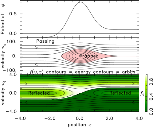
Figure 1: Schematic of a hypothetical asymmetric electron hole.

Fig. 1 illustrates schematically the potential, and electron and ion distribution function contours in their respective phase-spaces. There is a region of closed (trapped) electron orbits whose distribution function $f_{e}(x,v_{e})$ is set by the formation conditions of the structure. It is generally lower than the nearby untrapped (passing) $f_{e}$, which is set by boundary conditions and the constancy of $f$ on orbits, because of the Vlasov equation. The trapped electron deficit causes $n_{e}(x)<n_{i}(x)$ near $x=0$ and thereby sustains the potential $\phi$. The ion distribution is everywhere set by its value at the $x$-boundaries (infinity). In this illustration it is a Maxwellian shifted by 1.5 velocity units. The outgoing distribution is complicated by reflection and has discontinuities at the transition between reflected and unreflected orbits.

The problem addressed in the present work is this. Given prescribed electron and ion velocity distributions incoming at the boundaries, far from the potential structure, find a fully self-consistent electron hole equilibrium (with a local potential peak), and show how to calculate the electron hole velocity relationship to the distributions, the potential drop $\Delta\phi$, and the relationship between the hole potential and the trapped electron distribution function. Furthermore, establish the circumstances under which such an asymmetric equilibrium is stable.

In a recent publication[24], the equilibrium and stability of slow electron holes with symmetric and asymmetric ion distributions, and ion reflection, was analysed under the rather ad hoc assumption that the hole potential is symmetric. It was found that an essential ingredient of stability under this approximate ansatz was that $f_{i}(v)$ should be double humped. And this is in accord with recent space plasma observations[29]. The present purpose is to proceed instead without assuming the potential to be symmetric, and thereby to complete and validate the analysis of slow asymmetric electron holes. The findings substantially confirm the prior simplified analysis.

II Theory Background

In this paper the Vlasov equation will not actually be written down. Instead its property that the distribution function $f(v)$ is constant along orbits will be used directly. In a steady potential, the particle energy is also a constant of the motion, and so $f$ is a function of energy. Together with the knowledge that particle density is $n=\int fdv$ these facts are sufficient to analyze equilibria.

Bernstein, Greene, and Kruskal, in their original paper[1] showed that one can formally solve to find the required distribution functions to create any arbitrary mode potential shape $\phi(x)$, with an arbitrary number of minima and maxima, as follows. Dividing the spatial domain into segments between adjacent local minima and maxima ($\phi_{min}$ and $\phi_{max})$, consider the ions in a segment of increasing $\phi(x)$ and suppose their velocity distribution to be known for all relevant energy ${\cal E}_{i}\equiv{1\over 2}m_{i}v^{2}+e\phi>e\phi_{min}$ and the passing electron distribution to be known for ${\cal E}_{e}\equiv{1\over 2}m_{e}v^{2}-e\phi>-e\phi_{min}$. The electrons reflected from this potential segment $-e\phi_{max}<{\cal E}_{e}<-e\phi_{min}$, entering from the right, have a velocity distribution $f_{er}$ symmetric in $v$ and a function only of energy. Their density must satisfy Poisson’s equation $n_{er}(\phi)+n_{ep}(\phi)-n_{i}(\phi)={\epsilon_{0}\over e}{d^{2}\phi\over dx^{2}}$, where subscripts $r$ and $p$ refer to reflected and passing (unreflected) particles. Since $n_{er}=2\int_{0}^{v_{s}}f_{e}(v)dv=(2/m_{e})\int_{-e\phi_{max}}^{-e\phi_{min}}f_{e}({\cal E})/\sqrt{2({\cal E}+e\phi)}\,d{\cal E}$, and $n_{ep}(\phi)$, $n_{i}(\phi)$, and ${d^{2}\phi\over dx^{2}}$ are known, giving $n_{er}(\phi)$, an integral equation governs the reflected part of $f_{e}({\cal E})$ and can be solved to find the unique required trapped-electron distribution consistent with the specified potential profile. For the next segment to the right, which has decreasing $\phi(x)$, the roles of electrons and ions are reversed, the entire $f_{e}$ is known and the passing ion $f_{ip}$. One can thus find the required reflected ion distribution from an integral equation. By this sequential process one can in principle find the sequence of reflected (and trapped) distribution functions that self-consistently satisfy Poisson’s equation and dependence of $f(v)$ only on energy, i.e. the steady Vlasov equation.

Concerning a solitary potential structure like an electron hole, if the asymmetry $\Delta\phi$ becomes so great that it removes the local potential maximum, giving rise to a monotonic potential $\phi(x)$, and removing all local electron trapping, then the structure is called a Double-Layer. Double-layers have a long history of study since their first experimental observation and analysis by Langmuir[31]. Although the possibility of asymmetric solitons, with local potential minima or maxima has been noted in these and other double layer studies[2], almost all of the analysis assumes that the double-layer potential is monotonic or occasionally has a local minimum (i.e. an ion hole, or an electron-acoustic soliton[32]). A (monotonic) double-layer has a single potential segment, and the approach of BGK described in the previous paragraph describes how, given $\phi(x)$ and the entire incoming distribution of the reflected species on one side, the required distribution of the other species on the other side can be found. Variations around the BGK integral equation method appeared in the early development of double-layer analysis [33, 34]. They were joined by approaches that express the shape of the velocity distribution in terms of a few fluid-like parameters such as reflected species effective temperature and passing mean velocity. These often used what is essentially BGK’s differential equation method and the requirement of net charge and force neutrality in the form of boundary conditions for given potential drop $\Delta\phi$ (e.g.[35]). The influential model of Perkins and Sun[36], for example, showed that provided the passing particle distributions are chosen appropriately, no net electric current need flow across the double-layer, which had previously been in doubt; but their model had only one adjustable parameter governing the reflected ions, thereby constraining both $\Delta\phi$ and the trapped ion parameter to be unique functions of the passing electron to ion temperature ratio. One should beware of so called nonlinear dispersion relations like this; they arise because of artificially prescribing the shape of the trapped distribution. Double-layer analysis is well summarized in the extensive reviews of Raadu[37, 38] and their references.

An electron hole, though, such as illustrated in Fig. 1, has two segments and a single local potential maximum, thus occasionally being referred to as a “Triple-Layer”. Moreover, neither the double-layer analyses nor the BGK sequential integral equation approach show how to deal with a situation in which the incoming velocity distributions of the particles on either side of the potential structure are broad but known, and we wish to solve instead for the potential $\phi(x)$ when it is unknown. This is nearest to the situation encountered in space observations, on which most of the electron hole experimental research is currently focussed, and in which satellites generally measure the ion and electron distribution functions in the background plasma. It is also what is needed to initialize a consistent slow electron hole in a simulation with prescribed particle velocity distributions. And it is the subject of the present work. Our interest includes the stability of the electron hole velocity, which is vital in this context for a slow electron hole to persist. All of the considerations here are purely one-dimensional.

III Problem specification and approach

III.1 Specifying the ion distribution

We begin by supposing that the incoming ion velocity distribution far from the hole is known and the potential is steady in the rest frame of the hole. The distribution at arbitrary position $x$ is then governed by $f_{i}(x,v)=f_{i}(\infty,v_{\infty})$, with energy conserved along orbits giving total ion energy ${\cal E}=mv^{2}/2+e\phi=mv_{\infty}^{2}/2+\phi_{\infty}$, and $v_{\infty}$ and $\phi_{\infty}$ corresponding to whichever side of the hole the ion entered. Denote the sign of $x$ (the position relative to the potential peak at $x=0$) by $\sigma_{x}(=\pm 1)$. At $x$, all inward moving ions entered from the same side $\sigma_{\infty}=\sigma_{x}$; but outgoing ions entered from the other side $\sigma_{\infty}=-\sigma_{x}$ if they are passing, or the same side $\sigma_{x}$ if they have been reflected. The sign of the entering velocity ($v_{\infty}$) is of course $-\sigma_{\infty}$. So $v_{\infty}=-\sigma_{\infty}\sqrt{2({\cal E}-e\phi_{\infty})/m}=-\sigma_{\infty}\sqrt{v^{2}+2e(\phi-\phi_{\infty})/m}$, and consequently

$$\begin{split}n_{i}(x)=\int f_{i}(x,v)dv=\int f_{i}(\sigma_{\infty}\infty,-\sigma_{\infty}\sqrt{v^{2}+2e(\phi-\phi_{\infty})/m})\,dv.\end{split}$$ (1)

Evaluation of this integral requires knowledge of the peak potential height $\psi$ (at $x=0$) because outgoing ions of energy ${\cal E}<e\psi$ have been reflected, while those with ${\cal E}>e\psi$ have not. Thus $\sigma_{\infty}$ changes sign at ${\cal E}=e\psi$. This change generally causes a discontinuity in $f_{i}(x,v)$.

Figure 2: Illustration of ion distributions on either side of the potential hill, and their integral, which is the cumulative probability distribution $P(v)$, and equals $n_{i}(\phi)$ at $v=+\infty$.

Fig. 2 illustrates these features for an incoming ion velocity distribution consisting of the sum of two Maxwellians having density, mean velocity, and temperature respectively: $(0.3,1.5,1)$ and $(0.7,-1.5,1)$, and potential peak $\psi=0.09$. In the codes and this and all other plots we use units normalized to Debye length $\sqrt{\epsilon_{0}T_{0}/n_{i}e^{2}}$, reference ion thermal energy $T_{0}$ and thermal velocity $\sqrt{T_{0}/m_{i}}$, and densities are unity when $\phi=\psi=0$. In these units, the ion mass is 1 and the ion charge is $e=1$, and potential is in units $T_{0}/e$. The electron temperature $T_{e}$ is equal to $T_{0}$ unless otherwise noted. Recognize that $\phi_{\infty}$ is initially unknown, and different for different sides $\sigma_{\infty}$.

In view of the energy conservation that yields eq. (1), it seems best to regard $f_{i}(\infty)$ as a fixed function of energy ${\cal E}$ and velocity sign, regardless of $\phi_{\infty}$, so as to make the passing ion distribution independent of $\Delta\phi=\phi(+\infty)-\phi(-\infty)$. To do so requires us to prescribe $f_{i}(\infty)$ at some negative values of energy, since for non-zero $\Delta\phi$, when $\bar{\phi}_{i\infty}=(\phi(+\infty)+\phi(-\infty))/2$ is taken to be the zero of potential, the lower side’s potential becomes negative and we need the incoming ion distribution there down to zero velocity. We therefore regard a function $f_{i\infty}(v)$ to be prescribed, and take

$$f_{i}(\sigma_{\infty}\infty,{\cal E})=\begin{array}[]{ll}f_{i\infty}(-\sigma_{\infty}\sqrt{2{\cal E}/m})&\mbox{for}\quad{\cal E}\geq 0\\ f_{i\infty}(0)&\mbox{for}\quad{\cal E}<0.\end{array}$$ (2)

Then we will later display the chosen distant ion distributions by a plot of $f_{i\infty}(v)$.

III.2 Determining distant potential asymmetry

Knowledge of the incoming $f_{i}(\sigma_{\infty}\infty,-\sigma_{\infty}|v_{\infty}|)$ and $\psi$ is sufficient to determine also the distant outgoing distribution as a function of energy, when both of $\phi(\pm\infty)$ are known. The ion densities $n_{i\infty}(\sigma_{\infty}\infty,\psi)$ on either side then generally differ, and depend on $\psi$. Figure 3 illustrates the result for the same incoming ion distribution and potential peak height as Fig. 2.

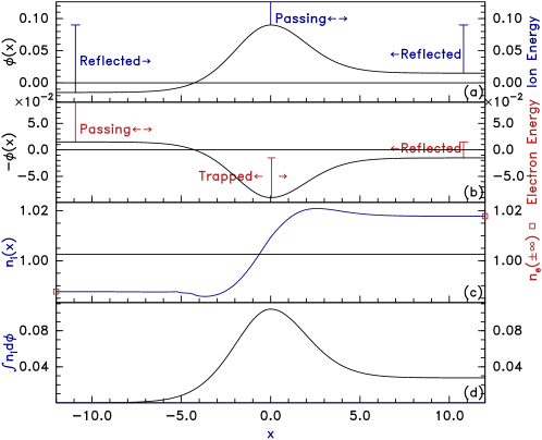
Figure 3: Illustrative asymmetric electron hole parameters (a) $\phi(x)$, which is ion potential energy; (b) $-\phi(x)$, electron potential energy; (c) $n_{i}(x)$ ion density; (d) ‘Classical’ potential giving force. The vertical bars in (a) and (b) indicate ranges of particle energy that are passing, reflected, or trapped. The two points in (c) show the matching distant electron density. The nonzero value of $\int_{-\infty}^{+\infty}n_{i}d\phi$ shows this hole is subject to non-zero ion force.

For a solitary structure like an electron hole, the plasma must be neutral ($n_{i\infty}-n_{e\infty}=0$) at distant positions on both sides, to bring the external potential curvature to zero. Consequently, if the electron distribution $f_{e}({\cal E}_{e})$ is known, and therefore $n_{e}(\phi)$ is a known fixed function, then the two simultaneous neutrality requirements are sufficient in principle to determine the two $\phi_{\infty}$ values. In practice it is convenient to choose the electron parameters so that $n_{e}(\phi)$ is an easily invertible function. A natural choice is to assume it has Boltzmann dependence $n_{e}\propto\exp(e\phi/T_{e})$, so

$$\Delta\phi=\phi_{i}(+\infty)-\phi_{i}(-\infty)=(T_{e}/e)\ln(n_{i}(+\infty)/n_{i}(-\infty)).$$ (3)

But for numerical solution one could make other choices. Indeed, one could consider electron distributions that are asymmetric in incoming velocity, so that when $\Delta\phi$ is non-zero, giving rise to electron reflection, the electron density then depends on $\sigma_{x}$ (as well as $\phi$). A treatment that performed the integration over specified electron distribution, like eq. (1), would then be required, imposing moderate extra computational effort.

In any case, since the distant ion density $n_{i}(\pm\infty)$ is itself a nonlinear function of $\phi(\pm\infty)$, $\Delta\phi$ solutions in general have to be found by iteration. In the present work it is assumed that $n_{e}=n_{e0}\exp(e\phi/T_{e})$. That is a good approximation for Maxwellian electrons and weak current density. We shall also take $\psi$ to be fixed relative to the mean $\bar{\phi}_{i\infty}=[\phi(+\infty)+\phi(-\infty)]/2$, which is taken to be the zero of potential. The difference $\Delta\phi$ evolves during solving iterations. Newton’s method applied to the residual $(T_{e}/e)\ln(n_{i}(+\infty)/n_{i}(-\infty))-\Delta\phi$ is observed to converge to numerical integration accuracy in fewer than 10 iterations. Once $\Delta\phi$ is converged, $n_{e0}$ is determined by $n_{e0}=n_{i}(\pm\infty)/\exp(\pm e\Delta\phi/2T_{e})$. This procedure produces potential limits that are consistent with the incoming ion and electron distributions and $\psi$. Fig. 3 illustrates the spatial dependencies using the converged $\Delta\phi$, when the hole velocity $v_{h}$ is zero in the ion frame.

III.3 Poisson’s equation and force balance

A full solution of a one-dimensional electron hole shape satisfies Poisson’s equation

$$\epsilon_{0}{d^{2}\phi\over dx^{2}}=-\rho,$$ (4)

where $\rho$ is the charge density $\rho=e(n_{i}-n_{e})$. When $\rho$ is a function only of potential not directly $x$, as is the case here, such a differential equation can be integrated once as $[{\epsilon_{0}\over 2}({d\phi\over dx})^{2}]_{\phi_{0}}^{\phi}=-\int_{\phi_{0}}^{\phi}\rho d\phi\equiv-V$; and the second integral $[x]_{\phi_{0}}^{\phi}=\pm\int_{\phi_{0}}^{\phi}\sqrt{\epsilon_{0}/2|V|}d\phi$ provides the solution in the form $x(\phi)$. In the soliton context, $V$ is often called the ‘Classical’ or ‘Sagdeev’ potential. The key boundary conditions of a solitary solution are that $V$ be zero at the extrema of $\phi$, including at $x\to\pm\infty$ where $dV/d\phi=e(n_{i}-n_{e})=0$ (just discussed) and $d^{2}V/d\phi^{2}\leq 0$ (to ensure the nearby $V$ is non-positive). Behind the mathematics, though [39], $V=\int\rho{d\phi\over dx}dx$ is physically minus the integrated force exerted on the charge by the electric field; and ${\epsilon_{0}\over 2}({d\phi\over dx})^{2}$ is the Maxwell stress, whose difference expresses the same quantity $V=-\int\epsilon_{0}{d^{2}\phi\over dx^{2}}{d\phi\over dx}dx=-\left[{\epsilon_{0}\over 2}\left(d\phi\over dx\right)^{2}\right]$. Fig. 3(d) shows the integration $\int n_{i}d\phi$ for ions alone, representing minus the force on the ions. For a symmetric electron hole (or other soliton) the forces on the two sides cancel by symmetry; but an asymmetric potential has no guaranteed force cancellation. And in fact the total force (per unit transverse area) $F$ will generally be non-zero, causing hole acceleration, except when the hole has a particular velocity relative to the specified incoming distributions. There is thus an additional criterion for a steady equilibrium that enforces a particular hole velocity so as to satisfy force balance. A symmetric-potential hole satisfies this criterion when it has zero or symmetric reflected particle velocity distribution in the hole frame. Fig. 3 in fact has non-zero $F$ and so does not satisfy force balance. It is not actually an equilibrium. The potential structure would be subject to acceleration.

Satisfying $F=0$ places no direct constraints on the trapped electron distribution, having energy $-e\psi\leq{\cal E}_{e}\leq-e|\Delta\phi/2|$. The reason is that trapping enforces symmetry of the distribution, so the trapped densities $n_{et}$ (and electron charge-densities) on the two sides of the potential peak at the same potential are equal, and the two contributions $-e\int n_{et}{d\phi\over dx}dx$ are equal and opposite (as are the passing electron contributions). The remaining contribution of electrons to $F$ arises from the integral of the electron density over $\Delta\phi$, that is

$$F_{e}=-V_{e}=e\int_{-\Delta\phi/2}^{\Delta\phi/2}n_{e}d\phi=n_{e0}T_{e}[\exp(e\Delta\phi/2T_{e})-\exp(-e\Delta\phi/2T_{e})].$$ (5)

It is the force of electron reflection from the potential difference across the hole, and for the present Maxwellian electrons is manifestly the electron pressure-difference across the hole.

The ion force also arises from reflection, in its case from either side of the potential hill, and since there are no trapped ions, it can be written simply

$$F_{i}=-\sum_{\sigma_{x}=\pm 1}\sigma_{x}e\int_{\phi(\sigma_{x}\infty)}^{\psi}n_{i}d\phi,$$ (6)

with $n_{i}$ given by eq. (1). If we regard the electron and ion distant distributions as given in the fixed ion frame, the only freedom we have to satisfy $F_{e}+F_{i}=0$ is to suppose that the hole moves with some velocity $v_{h}$ relative to that frame, and that $v_{h}$ is to be adjusted to satisfy force balance. This viewpoint is intuitive, since the result of a non-zero total force will in fact be hole acceleration, that is modification of $v_{h}$.

Thus, we must (again iteratively) search for a $v_{h}$ that gives $F=0$, when $\Delta\phi$ is given as in section III.2 by the requirements on $n(\pm\infty)$. The result will be to find $v_{h}$, $\Delta\phi$, that satisfy all the boundary conditions (including force balance), without any constraints (beyond symmetry) so far on the trapped electron distribution.

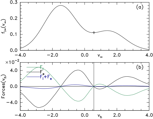
Figure 4: Distant velocity distribution of the ions ($f_{i\infty}$) and the composition of the forces exerted on the electrons and ions, as $v_{h}$ is varied.

Fig. 4 illustrates the search process graphically. Panel (a) simply plots, in the fixed ion frame, the distant ion velocity $f_{i\infty}(v_{\infty})$ distribution used for the examples we are giving. Panel (b) shows as a function of $v_{h}$ the total force on ions, electrons, and their sum, when $\Delta\phi$ is such that $n_{e}(\pm\infty)=n_{i}(\pm\infty)$, that is, distant neutrality is satisfied. Notice that there is substantial cancellation between $F_{i}$ and $F_{e}$. The total force $F_{i}+F_{e}$ given in blue is the critical quantity. Equilibria occur where it is zero. This scan shows that there are three such $v_{h}$ roots. However, at two of them, the ones located near the distribution maxima, the slope $dF/dv_{h}$ is positive. That sign means that at any adjacent velocity the non-zero force acts to accelerate the hole potential velocity $v_{h}$ away from the equilibrium value. Thus those equilibria are unstable to slow acceleration. Therefore the $F$ zero that is of interest is the middle one where $dF/dv_{h}<0$, and is selected by the scan for further refinement of the $v_{h}$ value. The vertical line and the cross on the $f_{i\infty}$ plot indicate that equilibrium value.

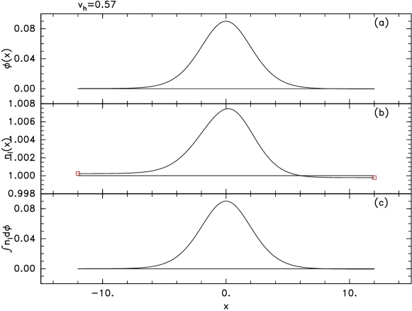
Figure 5: Converged equilibrium shape of potential $\phi(x)$, ion density $n_{i}(x)$ and ion force, when the hole required velocity $v_{h}=0.57$ for equilibrium has been discovered. For the same $\psi$ and $f_{i\infty}$ as before.

Fig. 5 shows the resulting potential, density and force distributions as a function of position when the hole speed corresponds to equilibrium. Now the total force is zero $\int_{-\infty}^{\infty}(n_{i}-n_{e}){d\phi\over dx}dx=0$, and to achieve this the shift of the hole-frame ion distribution (by $-v_{h}$) has almost (but not quite) symmetrized the densities and potentials: $n_{i}(+\infty)\simeq n_{i}(-\infty)$, $\phi(+\infty)\simeq\phi(-\infty)$. The remaining asymmetry of the distant ion density is cancelled by a very small potential difference changing the electron density. It should be emphasized that this near spatial symmetry only occurs at or near equilibrium. At $v_{h}$ values in Fig. 4 where the forces are large, there are much larger asymmetries in the three curves than Fig. 5 shows; compare Fig. 3, where $v_{h}=0$, for example.

III.4 Potential Shape

The shape $\phi(x)$ is so far undetermined except for the values of its extrema. We are therefore in the usual situation for BGK modes of having great liberty in the potential shape, depending on the velocity distribution of trapped electrons. (The $\phi(x)$ plots given so far should be considered illustrative of plausible possibilities.) The difference in potential $\Delta\phi$ is of course, induced by ion-density differences. So ions must be accounted for in relating the trapped electron distribution to $\phi(x)$. The simpler choice is to regard $\phi(x)$, rather than $f_{et}(v)$, as prescribed in the trapping region, and deduce the required trapped electron distribution by solving the integral equation that arises from setting $e(n_{i}-n_{e})=-\epsilon_{0}{d^{2}\phi\over dx^{2}}$. Naturally, there will be some constraints on the trapped distribution such as non-negativity and finite slope. But these should be no more difficult to satisfy than they are for symmetric holes. Moreover, it is not actually necessary to solve to find $f_{et}(v)$ in order to complete the hole structure determination, because it is only the trapped density $n_{et}(\phi)$ that is required.

We are, however, not now free to choose separately the $\phi(x)$ profiles on both sides of the hole ($\sigma_{x}=\pm 1$), because the trapped electron density at a particular potential is the same on both sides. The ion density is not symmetric, but is already prescribed on both sides. Let $\sigma_{\infty}=\sigma_{m}\equiv sign(\Delta\phi)$ denote the side with higher distant potential. Then there is no freedom to adjust the potential profile by trapped electron distribution choices at energies $-e\phi(\sigma_{m}\infty)<{\cal E}_{e}<-e\phi(-\sigma_{m}\infty)$, because those electrons are not trapped, they are reflected. If we freely prescribe the potential profile for side $\sigma_{x}=\sigma_{m}$, it determines the required trapped velocity distribution. But then the spatial profile on the other side ($\sigma_{x}=-\sigma_{m}$) must be found by solving Poisson’s equation there, because the trapped electron distribution has already been determined. By virtue of the way we chose $\Delta\phi$ and $v_{h}$ to satisfy equilibrium, all the boundary conditions on the $-\sigma_{m}$ side can be satisfied; that is, if we start the Poisson solution with $\phi=\psi$ and $d\phi/dx=0$ at $x=0$, we will find that $\phi(\infty)=-|\Delta\phi|/2$ and ${d\phi\over dx}|_{\infty}=0$. The natural way to solve for the entire profile is to use the implicit form $x=\pm\int_{\psi}^{\phi(x)}\sqrt{\epsilon_{0}/2|V|}d\phi$. This integration has been implemented numerically, and gives results consistent with the boundary conditions at infinity, to an accuracy dependent on the fineness of the integration grids.

The illustrative form of the potential prescribed on side $\sigma_{m}$ is chosen to be

$$\phi(x)=\phi_{\infty}+(\psi-\phi_{\infty}){\exp(L)+1\over\exp(L)+\cosh^{4}(x/4\lambda)},$$ (7)

where the adjustable parameter $L$ when positive is the approximate length of a flattened region at the top of the potential, and when negative rapidly suppresses flattening; and $\lambda$ controls the distant exponential decay, usually being the (generalized) Debye screening length. This yields electron trapped velocity distributions of approximately the (negative temperature $T_{et}$) Maxwellian form $\propto\exp(-{\cal E}/T_{et})$, when $L\to-\infty$[3].

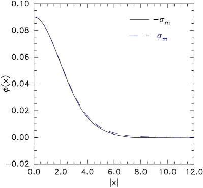
Figure 6: (a) Potentials on the two sides of the hole. Prescribed side dashed line, Poisson solution side solid. (b) Corresponding trapped electron distribution function at $x=0$, $\phi=\psi$.

Fig. 6(a) shows (for $L=-10$, $\lambda=1$ and the $f_{i\infty}$ of Fig. 4(a)) that the potential shape derived from the solution of Poisson’s equation (side $-\sigma_{m}$, solid curve) is very close to that for the prescribed side $\sigma_{m}$: eq. (7). The trapped electron distribution derived from solving the integral equation is shown in Fig. 6(b).

III.5 Stability to fast acceleration

In addition to the steady-state force imbalance already discussed, an additional mechanism that could give rise to hole velocity instability involves force imbalance arising from hole acceleration itself. An electron hole accelerating on the electron response timescale does not permit adjustment of the ion density fast enough to be effectively steady. As an approximation based on the separation of timescales, one can approach this issue by supposing there is negligible ion density change during some fast shift of the electron hole’s velocity and position from a full steady equilibrium. There would then arise a net force change of the hole potential on the ions (but by assumption not on the electrons) due to the shift displacement $\delta x$ of the potential structure from the original equilibrium, acting on the undisplaced ion density. For small displacements, the linearized change in potential at any position is $-{d\phi\over dx}\delta x$, giving rise to a change in force $\delta F=-e\delta x\int-{d^{2}\phi\over dx^{2}}n_{i}(x)dx=-e\delta x\int{d\phi\over dx}{dn_{i}\over dx}dx=-e\delta x\int{dn_{i}\over dx}d\phi$. Notice that the integral is of two (approximately) antisymmetric quantities ${d\phi\over dx}$ and ${dn_{i}\over dx}$, so it is finite regardless of potential shape, but has the sign of $-dn_{i}/d\phi$ of the dominant contributions to the integral. Stability depends on the sign of $\delta F/\delta x$, and therefore of the integral. If it is such as to enhance $\delta v_{h}$ and hence $\delta x$, which arises if $\delta F/\delta x$ is positive, exponential growth will occur. In so far as the system is correctly described dynamically by this shift motion with static ions, it will be stable if both $\delta F/\delta x$ and the equilibrium quantity $dF/dv_{h}$ are negative. Given the equilibrium solution, it is easy (numerically) to evaluate $\delta F/\delta x$, and it can be used to qualify an equilibrium’s dynamic as well as static stability.

Since the potential asymmetry is generally very small, and the $\delta F/\delta x$ depends only weakly on the $\phi(x)$ shape, it is usually sufficient to calculate it approximately using a model $\phi$ profile whose Poisson-solution side is approximated as equal to the specified-side’s $\phi(x)$ matched at $\phi=\psi$ with $\phi-\psi$ scaled to give the known $\Delta\phi$. That is what is plotted in figures 3 and 5. Varying the $x$-scale-length on either side makes no difference.

It is valuable to explore the existence of a stable equilibrium for a range of ion distribution shapes. One way to do this is to scale the velocity shift of each Maxwellian component (but not their width or density) by a range of factors. The result of such a set of calculations is shown in Fig. 7.

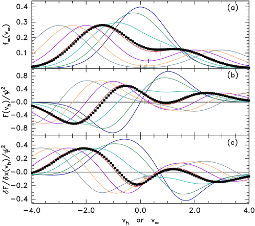
Figure 7: Stability parameters as a function of $v_{h}$, for a range of distributions obtained by scaling the Maxwellian components’ shift velocity.

It includes (a) the velocity distribution, $f_{i\infty}(v_{\infty})$ (b) the steady force $F(v_{h})$, and (c) the dynamic-shift force coefficient $\delta F/\delta x$ for a set of 7 different velocity shift scalings, colored by shift factor. The middle scaling factor is 1 (red) and corresponds to the distribution of the previous 5 figures. It confirms that $\delta F/\delta x$ is negative for the equilibrium $v_{h}$ shown by the cross, as previously found. Therefore by the approximate dynamic analysis this equilibrium is stable. For zero shift factor (blue) the ion distribution is a single Maxwellian. It’s equilibrium $F(v_{h})=0$ is unstable, and in such cases no cross is plotted. For a large shift factor of 2 (grey) the distribution consists of two components hardly overlapping. All distributions plotted from scale-factor of $\sim 1$ upward are stable. All below are unstable. A refined intermediate value of the scaling factor at the threshold for stability is found and plotted as black points with the corresponding equilibrium $v_{h}$ indicated by a short vertical line. It is noticeable that the static $dF/dv<0$ and dynamic $\delta F/\delta x$ stability thresholds are the same for this coarse scan. In other words (approximately): if and only if a distribution allows a statically stable equilibrium, it is dynamically stable. Moreover, it is required to have a local minimum in $f_{i\infty}$ in order for a stable equilibrium to exist. As has been shown previously[24], the larger the $\psi$ the deeper the minimum has to be. But for this moderate case, $\psi=0.09T_{0}$ (and smaller $\psi$), the depth required is small.

III.6 Summary of Algorithm and Numerical Implementation

The algorithm that has been implemented numerically is this.

1. From specified $f_{i\infty}(v_{\infty})$

— which is in principle arbitrary but is conveniently represented by a sum of shifted Maxwellian components of different densities and temperatures — and specified potential peak $\psi$, integrate equation (1), using equation (2) to obtain $n_{i}(\phi,\sigma_{x})$.

2. Determine the potential asymmetry $\Delta\phi$

using a search followed by Newton iteration of $\Delta\phi$, so as to satisfy equation (3). The algorithm of step 1 is used to give each iteration’s $n_{i}(\phi(\pm\infty),\sigma_{x})$.

3. Find the equilibrium hole velocity $v_{h}$

by searching, with repetitive use of step 2 to evaluate the total force $F$ exerted by the potential on particles. This is implemented by a coarse scan of $v_{h}$ (which provides data for explanatory plots such as Fig. 7) followed by iterative refinement of the precision of the equilibrium $v_{h}$ making $F=0$.

4. Construct the $\phi(x)$

by prescribing the higher potential side’s ($\sigma_{m}$) $\phi(x)$ using potential form eq. (7), giving the trapped electron density $n_{et}(\phi)$. Solve Poisson’s equation on the other side ($-\sigma_{m}$) using the then known $n_{i}(\phi)$, $n_{e}(\phi)$. Verify whether $\delta F/\delta x$ satisfies dynamic stability. If desired, solve the integral equation to find the trapped electron distribution function from the prescribed $\phi(x)$.

IV Asymmetric Holes at a range of parameters

We now illustrate asymmetric hole equilibria with $f_{i\infty}$ consisting of two shifted Maxwellian components, having densities $n_{1,2}$, temperatures $T_{1,2}$, and velocities in the reference (not hole) frame $v_{1,2}=\pm v_{s}$. The reference temperature is taken equal to the temperature of component one $T_{0}=T_{1}$, and the sum of the densities (the total background ion density) is unity $n_{1}+n_{2}=1$. Thus $n_{2}$, $T_{2}$, and $v_{s}$ are the three parameters determining the distribution shape. Fig. 8 surveys the shapes $f_{i\infty}(v)$ and resulting ion density profiles $n_{i}(x)$.

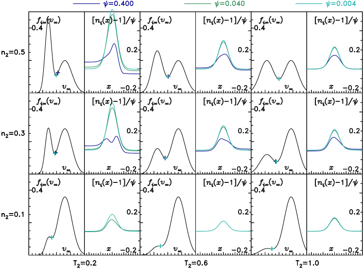
Figure 8: A 3$\times$3 display of 9 different cases $T_{2}$=$(.2,.6,1)$, $n_{2}$=$(.1,.3,.5)$ for which $v_{s}=0.75+\sqrt{T_{2}}$; here $T_{e}=T_{0}$. Each case has two adjacent subframe plots: the left-hand is $f_{i\infty}(v)$ and the right-hand represents scaled ion density perturbation as $[n_{i}(x)-1]/\psi$. All corresponding frames have the same axis ranges $-4\leq v_{\infty}\leq 4$, $-12\leq x\leq 12$. Densities are plotted for 3 different potential peak heights $\psi$=$(.4,.04,.004)$ indicated by different colors, but only if a stable equilibrium hole velocity ($v_{h}$) exists. If it does, a cross is plotted of that color on the left-hand subframe at that velocity and distribution height.

The overall scaling of the ion density perturbation is seen to be $n_{i}-1\sim\psi$. This is intuitive; the amplitudes of the potential perturbation and the density perturbation are proportional. We observe that there is very little difference in the scaled density perturbation between the lower amplitude cases $\psi=0.04,0.004$, even quantitatively. This is because for these cases the deficit in $f_{e}(v)$, and of $n_{i}$, supporting the hole, is fractionally small and can be linearized. By contrast, for $\psi=0.4$, the hole is deep and the ion density response is no longer linear. Moreover, for the bottom row, none of the distributions permits a stable hole at $\psi=0.4$ even though it does at the lower amplitudes. That is because deeper holes would require a deeper local minimum in $f_{i\infty}$ for stability than is provided by these cases.

The top right case ($T_{2}=1$, $n_{2}=0.5$) is completely symmetric, and the equilibrium is at $v_{h}=0$, the symmetry axis. Also there is no ion density difference across the hole and the corresponding potential difference $\Delta\phi=(T_{e}/e)\{\ln[n(+\infty)]-\ln[n(-\infty)]\}$ is zero. At lower values of $T_{2}$, substantial asymmetry in $n_{i}$ appears, becoming quite pronounced for $T_{2}=0.2$, (at the left) regardless of $n_{2}$ for the largest $\psi$. For smaller $\psi$, density $n_{i}(\infty)$ becomes more symmetric, although some small asymmetry remains, most noticeable at low $T_{2}$. Overall, though, the asymmetry in $n_{i}(\infty)$ at equilibrium remains less than $\sim 0.2\psi$, and in fact scales like $\psi^{2}$.

V Algebraic Calculation of Asymmetry

V.1 Explanation of approach

The scaling of potential asymmetry can be understood qualitatively as follows. We recognize that there are two types of asymmetric contribution to the neutrality requirement ($\Delta n_{e}=\Delta n_{i}$) and the force balance requirement ($F=0$). There is an intrinisic asymmetry arising even when $\Delta\phi=0$ that comes from the asymmetry of $f_{i\infty}$, and there is an extrinsic asymmetry that comes from $\Delta\phi$. The asymmetry (strictly antisymmetric part) of $f_{i\infty}$ can be expressed as the odd terms of its Taylor expansion in velocity in the hole frame $f^{\prime}v+{1\over 6}f^{\prime\prime\prime}v^{3}+O(v^{5})$, $f^{\prime}$ and $f^{\prime\prime\prime}$ are the first and third velocity-derivatives of $f_{i\infty}$ evaluated at $v=0$ (i.e. at ion-frame velocity $v_{h}$) taken as constants.

The intrinsic ion density asymmetry, which is to be evaluated between the positions on either side of the hole corresponding to $\phi=+|e\Delta\phi|/2$, has then two terms proportional respectively to $f^{\prime}\psi$ and $f^{\prime\prime\prime}\psi^{2}$. The $\psi$ dependences arise from integrals over $v$ to the hole height energy $v=\sqrt{2e\psi/m}$. There is no intrinsic electron density asymmetry because electrons are trapped by the positive potential peak, not reflected from it. The extrinsic density asymmetry arises from the change of $n_{e}$ and $n_{i}$, on the low potential side, across the range $-|\Delta\phi|/2\leq\phi\leq|\Delta\phi|/2$. These changes are both proportional to $\Delta\phi$, but with different coefficients.

The intrinsic ion force asymmetry likewise has two terms $\propto f^{\prime}\psi^{2}$ and $\propto f^{\prime\prime\prime}\psi^{3}$, where the additional power of $\psi$ (relative to $\Delta n$) comes from the integral $\int nd\phi$. There is no intrinsic electron force. The total extrinsic force arises from reflection of ions and electrons from the potential range $-|\Delta\phi|/2\leq\phi\leq|\Delta\phi|/2$, but it is most easily expressed as the difference in the Maxwell stress on the low potential side between $-|\Delta\phi|/2$ and $|\Delta\phi|/2$, which is simply $(\epsilon_{0}/2\lambda^{2})(\Delta\phi)^{2}$, where $\lambda$ is the length for generalized Debye screening including the response of both electrons and ions. Therefore the simplified structure of the simultaneous equilibrium requirements (writing coefficients $a,b,c,d$ to be found later) is

$$\begin{split}\Delta\phi&=a\psi f^{\prime}+bf^{\prime\prime\prime}\psi^{2}\\ \Delta\phi^{2}&=c\psi^{2}f^{\prime}+df^{\prime\prime\prime}\psi^{3}.\end{split}$$ (8)

Eliminating the $f^{\prime}$ terms,

$$\Delta\phi^{2}-{c\over a}\psi\Delta\phi-\left(d-{bc\over a}\right)f^{\prime\prime\prime}\psi^{3}=0,$$ (9)

which can be solved for $\Delta\phi$ as

$$\Delta\phi={c\psi\over 2a}\left[1\pm\sqrt{1+\left(d-{bc\over a}\right)\left(2a\over c\right)^{2}f^{\prime\prime\prime}\psi}\;\right].$$ (10)

The discriminant’s sign must be chosen to be opposite the sign of the first term. When $\Delta\phi/\psi$ is small, only the linear term is important in eq. 9, and

$$\Delta\phi\simeq\left(b-{ad\over c}\right)f^{\prime\prime\prime}\psi^{2}.$$ (11)

Thus both $\Delta\phi$ and $\Delta n_{i}$ scale $\sim\psi^{2}$, and also $\sim f^{\prime\prime\prime}$, which is the lowest order contribution to asymmetry in $f_{i\infty}$ about the local minimum where $f^{\prime}=0$. Actually the solution is not exactly at $f^{\prime}=0$, but it is at a value that makes the two equations consistent, which is

$$f^{\prime}=(\Delta\phi-bf^{\prime\prime\prime}\psi^{2})/a\psi\simeq-(d/c)f^{\prime\prime\prime}\psi.$$ (12)

And the distribution derivatives $f^{\prime}$ and $f^{\prime\prime\prime}$ must be evaluated at the $v_{h}$ value that satisfies this equation.

V.2 Intrinsic ion density asymmetry

To quantify our analytic asymmetry expressions we need to evaluate the $a,b,c,d$ coefficients used in eqs. (8) to (12), to relevant order in $\psi$ and $\Delta\phi/\psi$. Those equations have already assumed that $\psi$ is a small quantity to allow the $f_{i\infty}$ expansion; eq. 11 shows that $\Delta\phi/\psi=O(\psi)$; and eq. 12 shows that $f^{\prime}/f^{\prime\prime\prime}=O(\psi)$. In this section for brevity we introduce a notation for the equivalent velocity, $v_{\psi-\phi}=\sqrt{2e(\psi-\phi)/m}$, and in a similar way $v_{\phi}=\sqrt{2e\phi/m}$, $v_{\psi}=\sqrt{2e\psi/m}$, and $v_{\cal E}=\sqrt{2{\cal E}/m}=\sqrt{v^{2}+v_{\phi}^{2}}$. We also work in scaled units so that $e=1$, $m=1$, and $T_{0}=1$.

The intrinsic ion density asymmetry between two points on opposite sides of the potential peak, at the same potential $\phi$, is found from eq. (2). Noting that only for reflecting energies is there any asymmetry, we get

$$\Delta n_{f}(\phi)=2\int_{0}^{v_{\psi-\phi}}f_{i\infty}(-\sqrt{v^{2}+v_{\phi}^{2}})-f_{i\infty}(\sqrt{v^{2}+v_{\phi}^{2}})\,dv=2\int_{0}^{v_{\psi-\phi}}\Delta f_{i}dv.$$ (13)

Substituting the expansion for the antisymmetric part of $f_{i\infty}$, so that $\Delta f_{i}=-(2f^{\prime}v_{\cal E}+{1\over 3}f^{\prime\prime\prime}v_{\cal E}^{3})$ we have

$$\Delta n(\phi)=-2\int_{0}^{v_{\psi-\phi}}[2f^{\prime}(v^{2}+v_{\phi}^{2})^{1/2}+{1\over 3}f^{\prime\prime\prime}(v^{2}+v_{\phi}^{2})^{3/2}]dv.$$ (14)

Performing the integrals, we find

$$\begin{split}\Delta n(\phi)=&-2[v_{\psi-\phi}v_{\psi}+v_{\phi}^{2}\ln({v_{\psi-\phi}+v_{\psi}\over v_{\phi}})]f^{\prime}\\ &-{1\over 12}[v_{\psi-\phi}v_{\psi}(2v_{\psi}^{2}+3v_{\phi}^{2})+3v_{\phi}^{4}\ln({v_{\psi-\phi}+v_{\psi}\over v_{\phi}})]f^{\prime\prime\prime}.\end{split}$$ (15)

The lowest potential at which this applies is $\phi=|\Delta\phi|/2$, because on the higher side there are no lower potentials. Then $\Delta n_{f}=\Delta n(|\Delta\phi|/2)$ is the intrinsic contribution to the neutrality criterion. But because of the smallness of $\Delta\phi/\psi$, to lowest order we find a result independent of $\Delta\phi$.

$$\begin{split}\Delta n_{f}&=-2v_{\psi}^{2}f^{\prime}-{1\over 6}v_{\psi}^{4}f^{\prime\prime\prime}+O(v_{\psi}^{2}v_{|\Delta\phi/2|}^{2})\\ &=-4\psi f^{\prime}-{2\over 3}\psi^{2}f^{\prime\prime\prime}+O(\psi\phi)\end{split}$$ (16)

V.3 Intrinsic Ion Force

The integral of eq. (15) also provides us with the intrinsic force exerted by the potential on ions, $F_{f}=\int_{|\Delta\phi|/2}^{\psi}\Delta n(\phi)d\phi={1\over 2}\int_{v_{|\Delta\phi/2|}^{2}}^{v_{\psi}^{2}}\Delta n\;dv_{\phi}^{2}$. Closed form indefinite integrals exist:

$$\int v_{\psi-\phi}v_{\psi}+v_{\phi}^{2}\ln({v_{\psi-\phi}+v_{\psi}\over v_{\phi}})dv_{\phi}^{2}={1\over 2}[v_{\psi-\phi}v_{\psi}(-2v_{\psi}^{2}+v_{\phi}^{2})+v_{\phi}^{4}\ln({v_{\psi-\phi}+v_{\psi}\over v_{\phi}})]$$ (17)

and

$$\begin{split}&\int[v_{\psi-\phi}v_{\psi}(2v_{\psi}^{2}+3v_{\phi}^{2})+3v_{\phi}^{4}\ln({v_{\psi-\phi}+v_{\psi}\over v_{\phi}})]dv_{\phi}^{2}=\\ &\qquad\qquad\qquad{1\over 3}v_{\psi-\phi}v_{\psi}(-8v_{\psi}^{4}+2v_{\psi}^{2}v_{\phi}^{2}+3v_{\phi}^{4})+v_{\phi}^{6}\ln({v_{\psi-\phi}+v_{\psi}\over v_{\phi}}).\end{split}$$ (18)

Noting that the upper limits do not contribute because at $v_{\phi}=v_{\psi}$, $v_{\psi-\phi}=0$, the required definite integral becomes, to lowest order

$$\begin{split}F_{f}&=-v_{\psi}^{4}f^{\prime}+-{1\over 9}v_{\psi}^{6}f^{\prime\prime\prime}+O(v_{\psi}^{4}v_{|\Delta\phi/2|}^{2})\\ &=-4\psi^{2}f^{\prime}+-{1\over 9}8\psi^{3}f^{\prime\prime\prime}+O(\psi^{2}|\Delta\phi|).\end{split}$$ (19)

V.4 Extrinsic density difference and force

The neutrality condition requires in addition the change in $n_{i}-n_{e}$, which occurs between potentials $-|\Delta\phi|/2$ and $|\Delta\phi|/2$ on the lower $\phi_{\infty}$ side ($-\sigma_{m}$). It can be written

$$\Delta n_{\Delta\phi}=({dn_{i}\over d\phi}-{dn_{e}\over d\phi})\Delta\phi=-{\epsilon_{0}\over e}{\Delta\phi\over\lambda^{2}}.$$ (20)

The electron density change, since electrons are Maxwellian, is simply the Boltzmann factor, which gives ${dn_{e}\over d\phi}=n_{e0}e/T_{e}$. If this were the only source of charge, then Poisson’s equation would be ${d^{2}\phi\over dx^{2}}=\phi/\lambda_{De}^{2}$, where $1/\lambda_{De}^{2}=n_{e0}e^{2}/\epsilon_{0}T_{e}$ which in (the Debye) normalized units is $T_{0}/T_{e}$. Thus ${dn_{e}\over d\phi}e/\epsilon_{0}=1/\lambda_{De}^{2}=T_{0}/T_{e}$ gives the shielding length due to electrons alone; and we can write $-({dn_{i}\over d\phi}-{dn_{e}\over d\phi})e/\epsilon_{0}=1/\lambda^{2}=T_{0}/T_{s}=1/T_{s}$ (normalized) expressing the modified shielding length $\lambda$ including the linearized dielectric response of both electrons and ions in terms of an effective shielding temperature $T_{s}$ which is generally $\simeq T_{e}$.

Similarly, as previously noted, the extrinsic force on the particles can be expressed using $\lambda$ as the difference in the Maxwell stress in the range $-|\Delta\phi|/2$ ($|x|=\infty$) and $|\Delta\phi|/2$, in which the potential is exponential with decay length $\lambda$. Thus $|F_{\Delta\phi}|={\epsilon_{0}\over 2}\left(d\phi\over dx\right)^{2}={\epsilon_{0}\over 2\lambda^{2}}\Delta\phi^{2}$, with sign $\sigma_{\Delta}$ equal to that of $\Delta\phi$:

$$F_{\Delta\phi}=sign(\Delta\phi){1\over 2T_{s}}\Delta\phi^{2}\equiv\sigma_{\Delta}{1\over 2T_{s}}\Delta\phi^{2}.$$ (21)

V.5 Comparison with numerics

Dividing the neutrality $\Delta n_{\Delta\phi}+\Delta n_{f}=0$ and force balance $F_{\Delta\phi}+F_{f}=0$ conditions by minus the coefficients of their extrinsic terms $-1/T_{s}$ and $\sigma_{\Delta}/2T_{s}$, we obtain the coefficients for eq. (8):

$$\begin{array}[]{cc}a=4T_{s}&b={2\over 3}T_{s}\\ c=-8\sigma_{\Delta}T_{s}&d=-{16\over 9}\sigma_{\Delta}T_{s}\end{array}.$$ (22)

Substituting for them we find the potential asymmetry

$$\Delta\phi=\sigma_{\Delta}\psi(1-\sqrt{1-\sigma_{\Delta}(4T_{s}/9)f^{\prime\prime\prime}\psi})\simeq{T_{s}2\over 9}f^{\prime\prime\prime}\psi^{2}$$ (23)

and $f^{\prime}\simeq-{2\over 9}f^{\prime\prime\prime}\psi$. The density asymmetry is $\Delta n_{i}=\Delta n_{e}\simeq\Delta\phi/T_{e}=T_{s}/T_{e}{2\over 9}f^{\prime\prime\prime}\psi^{2}$.

The ion response ${dn_{i}\over d\phi}$ contribution to $T_{s}=({1\over T_{e}}-{dn_{i}\over d\phi})^{-1}$ is estimated on an ad hoc basis to be typically $0.3$. This estimate is probably the biggest fractional uncertainty unless $T_{e}$ is very small (in which case the ion contribution to shielding is small). Then we compare the present algebraic estimate with the numerical evaluation in Fig. 9(a) .

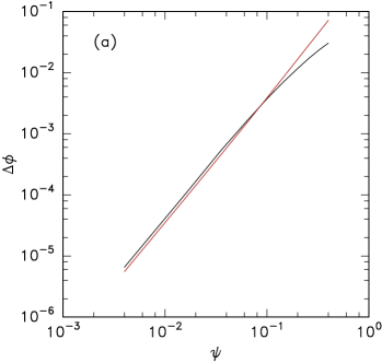
Figure 9: (a) Comparison of numerical (black) and algebraic (red) estimates of potential asymmetry $\Delta\phi$, showing its scaling proportional to the square of the electron hole peak potential $\psi$. In (b) is shown the ion distribution comprising Maxwellians $T_{1}=1$, $n_{1}=0.7$, $v_{1}=1.197$ $T_{2}=0.2$, $n_{2}=0.3$, $v_{2}=-1.197$, and $T_{e}=1$, in scaled units. The potential profiles in (c) are from the ends of the scaling range.

The good agreement between the two except in the region where $\psi$ is no longer small, is gratifying and serves as a verification of the numerical and algebraic integrations. The potential profiles Fig. 9(a) emphasize that even at the upper end of the scaling range (where the agreement is compromised by $\psi$ no longer being small) the asymmetry in the potential at equilibrium remains small. This case, corresponds to the $n_{2}=0.3$, $T_{2}=0.2$ case of Fig. 8, correcting any false impression given there by the density profiles that the potential asymmetry is strong. It never is.

VI Discussion

This numerical and algebraic analysis of asymmetric electron holes is, to my knowledge, the first that treats plausibly realistic external ion distributions taking into account the criteria of equilibrium. It shows that for truly solitary equilibrium positive potential structures, sustained by the plasma velocity distributions not imposed by local constraints, potential asymmetry is only minor, and for small amplitude electron holes is negligible. This finding moderates past speculations about asymmetric electron holes in the Double Layer literature. It also justifies and confirms the recent theory[24] of slow electron holes that ignores potential asymmetry. The present treatment remains purely an equilibrium theory, but the force on the hole out of equilibrium has been calculated, and its sign determines whether or not the equilibrium is stable. For a stable equilibrium to exist, the ion distribution must have a local minimum, and the hole velocity must lie within it.

It is possible for an electron hole to be formed at a velocity that does not satisfy the equilibrium force constraint, or in an ion distribution shape that causes any slow equilibrium to be unstable. If so, then it might initally have substantial potential asymmetry, or develop it during unstable acceleration. But once a hole finds a stable equilibrium velocity, that asymmetry will be largely suppressed. If, therefore, a substantially asymmetric electron hole were to be convincingly observed, its asymmetry might be an indication that it was young, dynamic, and still in the process of accelerating toward equilibrium. Of course, this treatment is also only one-dimensional, and all of its conclusions should be qualified by the possibility of being changed by multidimensional effects.

References

- Bernstein et al. [1957] I. B. Bernstein, J. M. Greene, and M. D. Kruskal, Exact nonlinear plasma oscillations, Physical Review 108, 546 (1957).
- Schamel [1986] H. Schamel, Electron holes, ion holes and double layers. Electrostatic Phase Space Structures in Theory and Experiment, Physics Reports 140, 161 (1986).
- Hutchinson [2017] I. H. Hutchinson, Electron holes in phase space: What they are and why they matter, Physics of Plasmas 24, 055601 (2017).
- Eliasson and Shukla [2006] B. Eliasson and P. K. Shukla, Formation and dynamics of coherent structures involving phase-space vortices in plasmas, Physics Reports 422, 225 (2006).
- Krasovsky et al. [2003] V. L. Krasovsky, H. Matsumoto, and Y. Omura, Electrostatic solitary waves as collective charges in a magnetospheric plasma: Physical structure and properties of Bernstein-Greene-Kruskal (BGK) solitons, Journal of Geophysical Research: Space Physics 108, 1117 (2003).
- Dupree [1982] T. H. Dupree, Theory of phase-space density holes, Physics of Fluids 25, 277 (1982).
- Turikov [1984] V. A. Turikov, Electron Phase Space Holes as Localized BGK Solutions, Physica Scripta 30, 73 (1984).
- Chen et al. [2004] L.-J. Chen, D. Thouless, and J.-M. Tang, Bernstein–Greene–Kruskal solitary waves in three-dimensional magnetized plasma, Physical Review E 69, 55401 (2004).
- Ng et al. [2006] C. S. Ng, A. Bhattacharjee, and F. Skiff, Weakly collisional Landau damping and three-dimensional Bernstein-Greene-Kruskal modes: New results on old problems, Physics of Plasmas 13, 55903 (2006), arXiv:1109.1353 .
- Hutchinson [2018] I. H. Hutchinson, Transverse instability of electron phase-space holes in multi-dimensional Maxwellian plasmas, Journal of Plasma Physics 84, 905840411 (2018), arXiv:1804.08594 .
- Hutchinson [2019] I. H. Hutchinson, Transverse instability magnetic field thresholds of electron phase-space holes, Physical Review E 99, 053209 (2019).
- Zhou and Hutchinson [2018] C. Zhou and I. H. Hutchinson, Dynamics of a slow electron hole coupled to an ion-acoustic soliton, Physics of Plasmas 25, 082303 (2018).
- Hutchinson [2021a] I. H. Hutchinson, Finite gyro-radius multidimensional electron hole equilibria, Physics of Plasmas 28, 052302 (2021a).
- Ergun et al. [1998] R. E. Ergun, C. W. Carlson, J. P. McFadden, F. S. Mozer, L. Muschietti, I. Roth, and R. J. Strangeway, Debye-Scale Plasma Structures Associated with Magnetic-Field-Aligned Electric Fields, Physical Review Letters 81, 826 (1998).
- Ergun et al. [1999] R. E. Ergun, C. W. Carlson, L. Muschietti, I. Roth, and J. P. McFadden, Properties of fast solitary structures, Nonlinear Processes in Geophysics 6, 187 (1999).
- Malaspina et al. [2013] D. M. Malaspina, D. L. Newman, L. B. Willson, K. Goetz, P. J. Kellogg, and K. Kerstin, Electrostatic solitary waves in the solar wind: Evidence for instability at solar wind current sheets, Journal of Geophysical Research: Space Physics 118, 591 (2013).
- Malaspina et al. [2014] D. M. Malaspina, L. Andersson, R. E. Ergun, J. R. Wygant, J. W. Bonnell, C. Kletzing, G. D. Reeves, R. M. Skoug, and B. A. Larsen, Nonlinear electric field structures in the inner magnetosphere, Geophysical Research Letters 41, 5693 (2014).
- Malaspina et al. [2018] D. M. Malaspina, A. Ukhorskiy, X. Chu, and J. Wygant, A census of plasma waves and structures associated with an injection front in the inner magnetosphere, Journal of Geophysical Research: Space Physics 123, 2566 (2018), https://agupubs.onlinelibrary.wiley.com/doi/pdf/10.1002/2017JA025005 .
- Malaspina and Hutchinson [2019] D. M. Malaspina and I. H. Hutchinson, Properties of Electron Phase Space Holes in the Lunar Plasma Environment, Journal of Geophysical Research: Space Physics 124, 4994 (2019).
- Steinvall et al. [2019] K. Steinvall, Y. V. Khotyaintsev, D. B. Graham, A. Vaivads, P.-A. Lindqvist, C. T. Russell, and J. L. Burch, Multispacecraft analysis of electron holes, Geophysical Research Letters 46, 55 (2019), https://agupubs.onlinelibrary.wiley.com/doi/pdf/10.1029/2018GL080757 .
- Graham et al. [2016] D. B. Graham, Y. V. Khotyaintsev, A. Vaivads, and M. André, Electrostatic solitary waves and electrostatic waves at the magnetopause, Journal of Geophysical Research: Space Physics 121, 3069 (2016).
- Tong et al. [2018] Y. Tong, I. Vasko, F. S. Mozer, S. D. Bale, I. Roth, A. V. Artemyev, R. Ergun, B. Giles, P. A. Lindqvist, C. T. Russell, R. Strangeway, and R. B. Torbert, Simultaneous Multispacecraft Probing of Electron Phase Space Holes, Geophysical Research Letters 45, 11,513 (2018).
- Lotekar et al. [2020] A. Lotekar, I. Y. Vasko, F. S. Mozer, I. Hutchinson, A. V. Artemyev, S. D. Bale, J. W. Bonnell, R. Ergun, B. Giles, Y. V. Khotyaintsev, P.-A. Lindqvist, C. T. Russell, and R. Strangeway, Multisatellite mms analysis of electron holes in the earth’s magnetotail: Origin, properties, velocity gap, and transverse instability, Journal of Geophysical Research: Space Physics 125, e2020JA028066 (2020), e2020JA028066 10.1029/2020JA028066, https://agupubs.onlinelibrary.wiley.com/doi/pdf/10.1029/2020JA028066 .
- Hutchinson [2021b] I. H. Hutchinson, How can slow plasma electron holes exist?, Phys. Rev. E 104, 015208 (2021b), http://arxiv.org/abs/2104.13800 .
- Eliasson and Shukla [2004] B. Eliasson and P. K. Shukla, Dynamics of electron holes in an electron-oxygen-ion plasma., Physical Review Letters 93, 45001 (2004).
- Zhou and Hutchinson [2016] C. Zhou and I. H. Hutchinson, Plasma electron hole kinematics. II. Hole tracking Particle-In-Cell simulation, Physics of Plasmas 23, 82102 (2016).
- Saeki and Genma [1998] K. Saeki and H. Genma, Electron-Hole Disruption due to Ion Motion and Formation of Coupled Electron Hole and Ion-Acoustic Soliton in a Plasma, Physical Review Letters 80, 1224 (1998).
- Zhou and Hutchinson [2017] C. Zhou and I. H. Hutchinson, Plasma electron hole ion-acoustic instability, J. Plasma Phys. 83, 90580501 (2017), arXiv:arXiv:1701.03140v1 .
- Kamaletdinov et al. [2021] S. R. Kamaletdinov, I. H. Hutchinson, I. Y. Vasko, A. Artemyev, A. Lotekar, and F. Mozer, Spacecraft observations and theoretical understanding of slow electron holes, Phys. Rev. Lett. (submitted) (2021).
- Note [1] In this work we will distinguish between trapping and reflection. A reflected particle escapes to large distance; a trapped particle does not, being confined by a local potential energy minimum.
- Langmuir [1929] I. Langmuir, The interaction of electron and positive ion space charges in cathode sheaths, Phys. Rev. 33, 954 (1929).
- Vasko et al. [2017] I. Y. Vasko, O. V. Agapitov, F. S. Mozer, J. W. Bonnell, A. V. Artemyev, V. V. Krasnoselskikh, G. Reeves, and G. Hospodarsky, Electron-acoustic solitons and double layers in the inner magnetosphere, Geophysical Research Letters 44, 4575 (2017), https://agupubs.onlinelibrary.wiley.com/doi/pdf/10.1002/2017GL074026 .
- Montgomery and Joyce [1969] D. Montgomery and G. Joyce, Shock-like solutions of the electrostatic vlasov equation, Journal of Plasma Physics 3, 1 (1969).
- Knorr and Goertz [1974] G. Knorr and C. K. Goertz, Existence and stability of strong potential double layers, Astrophysics and Space Science 31, 209 (1974).
- Schamel and Bujarbarua [1983] H. Schamel and S. Bujarbarua, Analytical double layers, Physics of Fluids 26, 190 (1983).
- Perkins and Sun [1981] F. W. Perkins and Y. C. Sun, Double layers without current, Physical Review Letters 46, 115 (1981).
- Raadu [1989] M. A. Raadu, The physics of double layers and their role in astrophysics, Physics reports 178, 25 (1989).
- Raadu and Rasmussen [1988] M. A. Raadu and J. J. Rasmussen, Dynamical aspects of electrostatic double layers, Astrophysics and Space Science 144, 43 (1988).
- Andrews and Allen [1971] J. G. Andrews and J. E. Allen, Theory of a double sheath between two plasmas, Proceedings of the Royal Society of London. Series A, Mathematical andPhysical Sciences 320, 459 (1971).
- Note [2] The structure of the second (force) equation of (8) puts two terms that are intrinsically of order equal to a left hand side of order which at equilibrium is of order . Therefore it might seem that we must keep terms up to ; that is, the terms containing a single factor . However, the elimination process with the first equation of (8) shows those terms are of order smaller in calculating , and they can safely be ignored, as has been verified by numerical evaluation including the higher order terms.
- Note [3] The code that produced the figures in this paper is available at https://github.com/ihutch/asymhill.