$f({\sf R})$ Gravity Wormholes sourced by a Phantom Scalar Field

Abstract

We derive an exact wormhole spacetime supported by a phantom scalar field in the context of $f({\sf R})$ gravity theory. Without specifying the form of the $f({\sf R})$ function, the scalar field self-interacts with a mass term potential which is derived from the scalar equation and in the resulting $f({\sf R})$ model the scalar curvature is modified by the presence of the scalar field and it is free of ghosts and avoids the tachyonic instability.

I Introduction

Wormholes in General Relativity (GR) are solutions of Einstein equations presenting hypothetical tunnels connecting different parts of the Universe or two different Universes. The first discussion of a wormhole configuration was presented by Flamm [1] and later by Einstein and Rosen (ER) introducing the “ER bridge”, a physical space being connected by a wormhole-type solution [2]. The wormhole spacetimes as solutions of GR were further investigated in the pioneering articles of Misner and Wheeler [3] and Wheeler [4].

Introducing a static spherically symmetric metric the necessary conditions to generate traversable Lorentzian wormholes as exact solutions in GR were first found by Morris and Thorne [5]. In these structures a condition on the wormhole throat necessitates the introduction of exotic matter, which however leads to the violation of the null energy condition (NEC). This type of matter has been discussed in cosmological contexts [6], for possible observational applications. Recently, it was found in [7] that normal Dirac and Maxwell fields can support wormhole configurations and provide violation only of the NEC. Many wormhole solutions were discussed in the literature. To avoid the violation of NEC in [8] the construction of thin-shell wormholes was studied, where ordinary matter is concentrated on the wormhole throat. Recently, there are many studies of wormhole solutions in modified gravity theories like Brans-Dicke theory [9], mimetic theories [10], $f({\sf R})$ gravity [11], Einstein-Gauss-Bonnet theory [12], Einstein-Cartan theory and general scalar-tensor theories [13]. Wormholes with AdS asymptotics have also been discussed [14] in an attempt to describe the physics of closed universes. Canonical scalar fields in the Horndeski scenario have also been used to constract wormhole geometries [15, 16, 17]. In these theories, their gravitational echoes have been recently investigated [18], while the formation of bound states of scalar fields in AdS-asymptotic wormholes were studied in [19]. A phantom scalar field was introduced in the Einstein-Hilbert action and wormhole solutions have been found by Ellis in [20], known as Ellis wormholes. Lately, several generalizations were obtained [21, 22, 23, 24, 25]. Phantom matter was considered in Einstein-Maxwell dilaton theory and wormholes have been constructed in [26].

The need to describe the early and late cosmological history of our Universe promoted the study of $f({\sf R})$ theories of gravity [27, 28, 29, 30, 31, 32, 33, 34, 35]. The main motivation to study these theories were the recent cosmological observational results on the deceleration-acceleration transition of late Universe. This requirement imposed constraints on the $f({\sf R})$ models allowing viable choices of $f({\sf R})$ [36]. These theories exclude contributions from any curvature invariants other than $\sf R$ and they avoid the Ostrogradski instability [37, 38].

Black holes in $f({\sf R})$ gravity theories with constant and non-constant Ricci curvature in vaccum or coupled to electrodynamics have been found [39]- [53] while in [54, 55, 56] scalar fields are introduced as matter in $(2+1)$ and $(3+1)$-dimensional $f({\sf R})$ gravity and the corresponding black hole solutions are investigated. This particular type of theory, $f({\sf R})$ gravity and non-minimally coupled scalar fields as matter has been previously considered for cosmological purposes [57, 58].

In [55] an exact black hole solution in $(2+1)$-dimensions of a scalar field minimally coupled to gravity in the context of $f({\sf R})$ gravity was found. Without specifying the form of the $f({\sf R})$ function, an exact black hole solution was obtained dressed with a scalar hair and the scalar charge to appear both in the metric and in the $f({\sf R})$ function. It was showed that thermodynamical and observational constraints required that the pure $f({\sf R})$ theory should be builded with a phantom scalar field. The reason for this behaviour is that the entropy in the $f({\sf R})$ theories receives an extra contribution and to have a positive entropy a contribution from phantom scalar field is required. Then, computing the Hawking temperature and the Bekenstein-Hawking entropy it was found that they are both positive, with the temperature getting smaller with the increase of the scalar charge while the entropy behaves the opposite way, growing with the increase of the scalar charge.

Wormhole solutions in $f({\sf R})$ theory have been constructed in [59], where the matter threading the wormhole is a fluid that satisfies the energy conditions, so the violation of the energy conditions comes from the higher order terms that the $f({\sf R})$ theory possesses. Thin-shell wormholes with circular symmetry in $(2+1)$-dimensional $f({\sf R})$ theories of gravity, with constant Ricci scalar have been investigated [60], while $(3+1)$-dimensional thin-shell wormholes in $f({\sf R})$ gravity with charge and constant curvature were discussed in [61], investigating also their stability. In quadratic $f(\sf R)=\sf R+\alpha\sf R^{2}$ gravity spherically symmetric Lorentzian wormholes have been found with a constant scalar curvature [62]. Using the Karmarkar condition wormhole geometries have been investigated in several $f({\sf R})$ models [63]. In [64] wormholes with a kinetic curvature scalar were considered and in [65] traversable $f({\sf R})$ gravity wormholes with constant and dynamic redshift function were found. Finally in [66] wormholes in $f({\sf R})$-massive gravity were investigated employing several behaviors for the redshift function, and wormholes in generalized hybrid metric-Palatini gravity that satisty the NEC were obtained [67].

In $f({\sf R})$ gravity theories if a conformal transformation is applied from the Jordan frame to the Einstein frame then, a new scalar field appears and also a scalar potential is generated. The resulted theory can be considered as a scalar-tensor theory with a geometric (gravitational) scalar field which however cannot dress a $f({\sf R})$ black hole with hair [68, 69, 70]. In our previous work [55, 56] the motivation for constructing hairy black hole solutions in $f({\sf R})$ gravity theories was to introduce a scalar field in the action as a matter field in the way it was done in the GR context and study its effect on a metric ansatz solving the field equations. In these models the scalar field was a canonical scalar field with positive kinetic energy.

In this work we follow a similar approach. We would like to investigate if we introduce a scalar field with negative kinetic energy (phantom scalar field) with a self-interacting potential, a wormhole configuration can be generated. In the literature in most of the studied models, the phantom matter is introduced in the energy-momentum tensor with a phantom equation of state violating the NEC. In our study we introduce explicitly a self-interacting phantom field and without specifying the form of the $f({\sf R})$ function, we solve the resulting field equations. To do that we have to specify the form of the phantom field and we find a new wormhole geometry sourced by the phantom scalar field which is free of ghosts and avoids the tachyonic instability and we show that the NEC is violated.

This work is organized as follows. In Section II we set up our theory, derive the field equations and discuss the restrictions a geometry has to obey to represent a wormhole configuration. In Section III we briefly discuss the GR case of a wormhole sourced by a phantom scalar field, the Ellis Drainhole [20] and we obtain a new wormhole geometry sourced by a phantom scalar field in $f({\sf R})$ gravity discussing also the energy conditions. Finally, in Section IV we conclude and we discuss possible extensions for further work.

II The setup-derivation of the field equations

We consider the following action

$$S=\int d^{4}x\sqrt{-g}\left(\frac{f(R)}{2}+\frac{1}{2}\partial^{\mu}\phi\partial_{\mu}\phi-V(\phi)\right)~{},$$ (1)

which consists of an arbitrary differentiable function of the Ricci Scalar $f(R)$, a scalar field with negative kinetic energy and a self-interacting potential.

The field equations that arise by variation of this action are

$$R_{\mu\nu}f_{R}(R)-\frac{1}{2}g_{\mu\nu}f(R)+\Big{(}g_{\mu\nu}\Box-\nabla_{\mu}\nabla_{\nu}\Big{)}f_{R}(R) = T_{\mu\nu}^{\phi}~{},$$ (2)

$$\Box\phi+V_{\phi}(\phi) = 0~{},$$ (3)

where $\Box=\nabla^{\mu}\nabla_{\mu}$ is the D’Alambert operator with respect to the metric, $f_{R}(R)=df(R)/dR$ and the energy momentum tensor is given by

$$T_{\mu\nu}^{\phi}=-\partial_{\mu}\phi\partial_{\nu}\phi+\frac{1}{2}g_{\mu\nu}\partial^{\alpha}\phi\partial_{\alpha}\phi-g_{\mu\nu}V(\phi)~{}.$$ (4)

We consider the following metric ansatz firstly used by Morris and Thorne [5] in spherical coordinates

$$ds^{2}=-e^{2\Phi(r)}dt^{2}+\left(1-\frac{b(r)}{r}\right)^{-1}dr^{2}+r^{2}d\Omega~{},$$ (5)

where $\Phi(r)$ is the redshift function and $b(r)$ is the shape function and $d\Omega=d\theta^{2}+\sin(\theta)^{2}d\varphi^{2}$. In order to obtain a wormhole geometry, these functions have to satisfy the following conditions [5, 71], namely:

1. $\frac{b(r)}{r}\leq 1$ for every $[r_{th},+\infty)$, where $r_{th}$ is the radius of the throat. This condition ensures that the proper radial distance defined by $l(r)=\pm\int_{r_{th}}^{r}\left(1-\frac{b(r)}{r}\right)^{-1}dr$ is finite everywhere in spacetime. Note that in the coordinates $(t,l,\theta,\phi)$ the line element (5) can be written as

   $$ds^{2}=-e^{2\Phi(l)}dt^{2}+dl^{2}+r^{2}(l)(d\theta^{2}+\sin^{2}\theta d\varphi)\,.$$ (6)

   In this case the throat radius would be given by $r_{th}=\min\{r(l)\}$.

2. $\frac{b(r_{th})}{r_{th}}=1$ at the throat. This relation comes from requiring the throat to be a stationary point of $r(l)$. Equivalently, one may arrive at this equation by demanding the embedded surface of the wormhole to be vertical at the throat.

3. $b^{\prime}(r)<\frac{b(r)}{r}$ which reduces to $b^{\prime}(r_{th})\leq 1$ at the throat. This is known as the flare-out condition since it guarantees $r_{th}$ to be a minimum and not any other stationary point.

Moreover, to simplify the calculations and to ensure the absence of horizons we will consider the case $\Phi(r)=C$ as in [59], where $C$ is a constant. Computing the $tt,rr,\theta\theta$ and the Klein-Gordon equations we find

$$rb^{\prime}f^{\prime}_{R}+3bf^{\prime}_{R}+2r(b-r)f^{\prime\prime}_{R}-rb\phi^{\prime 2}-4rf^{\prime}_{R}+r^{2}f-2r^{2}V+r^{2}\phi^{\prime 2}=0~{},$$ (7)

$$2f_{R}\left(b-rb^{\prime}\right)+4r(b-r)f^{\prime}_{R}+r^{2}(b-r)\phi^{\prime 2}+r^{3}(f-2V)=0~{},$$ (8)

$$r\left(r\left(\left(b^{\prime}-2\right)f^{\prime}_{R}+r\left(-2f^{\prime\prime}_{R}+f-2V+\phi^{\prime 2}\right)\right)-f_{R}b^{\prime}\right)-b\left(r\left(-f^{\prime}_{R}-2rf^{\prime\prime}_{R}+r\phi^{\prime 2}\right)+f_{R}\right)=0$$ (9)

$$\frac{\left(r\left(b^{\prime}-4\right)+3b\right)\phi^{\prime}+2r(b-r)\phi^{\prime\prime}}{2r^{2}}-\frac{V^{\prime}}{\phi^{\prime}}=0~{},$$ (10)

where primes denote derivative with respect to the argument, the radial co-ordinate $r$ and $f=f(R)=f(r)$, the gravitational model as a function of the radial co-ordinate $r$. Eliminating $f$ from equation (7) we obtain

$$f=2V-\frac{\left(r\left(b^{\prime}-4\right)+3b\right)f^{\prime}_{R}+r(r-b)\left(\phi^{\prime 2}-2f^{\prime\prime}_{R}\right)}{r^{2}}~{}.$$ (11)

Now substituting $f$ back to equations (8) and (9) we can obtain the following equations

$$r\left(r\left(b^{\prime}f^{\prime}_{R}-2rf^{\prime\prime}_{R}+2r\phi^{\prime 2}\right)+2f_{R}b^{\prime}\right)-b\left(r\left(f^{\prime}_{R}-2rf^{\prime\prime}_{R}+2r\phi^{\prime 2}\right)+2f_{R}\right)=0~{},$$ (12)

$$r\left(f_{R}b^{\prime}-2rf^{\prime}_{R}\right)+b\left(2rf^{\prime}_{R}+f_{R}\right)=0~{}.$$ (13)

As can be seen in equation (13), there is is a direct relation between the geometry and the $f(R)$ gravity, while the scalar field will affect both the $f(R)$ function and the geometry as we can see in equation (12).

III Wormhole Solutions

In this Section we will discuss the wormhole solutions of the field equations. We will first review the Ellis Drainhole.

III.1 The Ellis Drainhole

The Ellis Drainhole [20] is a wormhole solution of an action that consists of a pure Einstein-Hilbert term and a scalar field with negative kinetic energy

$$S=\int d^{4}x\sqrt{-g}\left(\frac{R}{2}+\frac{1}{2}\partial^{\mu}\phi\partial_{\mu}\phi\right)~{}.$$ (14)

Assuming the metric ansatz (5), setting in equations (7),(8),(9) calculated above $f(r)=R(r),f_{R}(r)=1,V(r)=0$ we obtain the following solution

$$b(r) = A^{2}/r~{},$$ (15)

$$\phi(r) = \sqrt{2}\tan^{-1}\left(\frac{\sqrt{r^{2}-A^{2}}}{A}\right)+\phi_{\infty}~{},$$ (16)

$$f(r) = R(r)=-\frac{2A^{2}}{r^{4}}~{},$$ (17)

where $A,\phi_{\infty}$ are two constants of integration. The resulting spacetime is asymptotically flat as it can be seen from both $b(r)$ and $R(r)$. The wormhole throat is the solution of the equation

$$g_{rr}^{-1}=0\rightarrow r_{th}=\pm A~{}.$$ (18)

The solution also satisfies the flaring-out condition and $b^{\prime}(r_{th})=-1$.

The scalar field takes a constant value at infinity $\phi(r\to\infty)=\frac{\pi}{\sqrt{2}}+\phi_{\infty}$, so one could set $\phi_{\infty}=-\frac{\pi}{\sqrt{2}}$ to make the scalar field vanish at large distances. However, since only derivatives of the scalar field appear in the field equations, its asymptotic value $\phi_{\infty}$ does not change the physical interpretation of the solution. The scalar field takes the asymptotic value at infinity at the position of the throat $\phi(r=r_{th})=\phi_{\infty}$. As can be seen in the solution (15), (16) and (17) the integration constant $A$ of the phantom scalar field plays a decisive role in the formation of the wormhole geometry. It has units $[L]$, appears in the scalar curvature and at the position of the throat takes the value $R_{r=r_{\text{th}}}(A)=-2/A^{2}$. Also it controls the size of the throat, a larger charge $A$ gives a larger wormhole throat.

The above results indicate that the presence of the phantom scalar field sources the wormhole geometry defining the scalar curvature and specifying the throat of the wormhole geometry. As we will see in the next Section if the scalar curvature is generalized to a general $f({\sf R})$ function, the phantom scalar field sources the wormhole geometry.

III.2 $f(R)$ Gravity Phantom Wormhole

A generalization of the Ellis Drainhole solution is to introduce a potential for the scalar field. Then we consider the full action (1) from which we obtain the field equations (2) and (3). To solve them we consider the metric ansatz (5). As we discussed in Section (II) the field equations resulting from action (1) are (10), (12) and (13). These equations constitute a system of three independent differential equations for the four unknown functions: $b(r),~{}f_{R}(r),~{}V(r),~{}\phi(r)$, therefore in principle we have to fix one of the unknown functions to solve for the others. One can also see that equation (10) can be obtained by taking the covariant derivative of equation (2). We found that for a particular scalar field configuration we can obtain a rather simple solution. Therefore we fix

$$\phi(r)=\sqrt{6}\frac{\sqrt{A}}{r}~{},$$ (19)

where $A>0$ is a constant which has dimensions $[L]^{2}$. Then solving the equations (12), (13) and (10) we get

$$b(r) = \frac{c_{1}r^{3}}{A^{2}}+2r~{},$$ (20)

$$f_{R}(r) = \frac{A}{r^{2}}~{},$$ (21)

$$V(r) = -\frac{3c_{1}}{Ar^{2}}~{},$$ (22)

$$f(r) = \frac{2A}{r^{4}}~{},$$ (23)

$$R(r) = \frac{6c_{1}}{A^{2}}+\frac{4}{r^{2}}~{},$$ (24)

$$f(R) = \frac{\left(A^{2}R-6c_{1}\right)^{2}}{8A^{3}}~{},$$ (25)

$$V(\phi) = -\frac{c_{1}\phi^{2}}{2A^{2}}~{},$$ (26)

where $c_{1}$ is a constant of integration with units $[L]^{2}$ in order $b(r)/r$ to be dimensionless. We can see that the resulting potential is a mass term potential, hence we set: $c_{1}=-A^{2}m^{2}$ and now the configurations become

$$b(r) = 2r-m^{2}r^{3}~{},$$ (27)

$$V(r) = \frac{3Am^{2}}{r^{2}}~{},$$ (28)

$$R(r) = \frac{4}{r^{2}}-6m^{2}~{},$$ (29)

$$f(R) = \frac{1}{8}A\left(6m^{2}+R\right)^{2}~{},$$ (30)

$$V(\phi) = \frac{1}{2}m^{2}\phi^{2}~{}.$$ (31)

To understand the physical meaning of the constants entering the solution of the field equations we found, let us rewrite the action (1) using the solution we found

$$S=\int d^{4}x\sqrt{-g}\left(\frac{1}{16}A\left(6m^{2}+R\right)^{2}+\frac{1}{2}\partial^{\mu}\phi\partial_{\mu}\phi-\frac{1}{2}m^{2}\phi^{2}\right)~{},$$ (32)

where the scalar field is given by (19). We can see that the constant $A$ which enters in the choice of the scalar field (19) is giving a mass to the scalar field and in the same time modifies the Ricci scalar curvature by a non-linear correction term. On the other hand it also contributes to the size of the throat of the wormhole as can be seen in (20).

This solution is a generalization of the Ellis wormhole solution discussed in the previous subsection. In this solution the scalar curvature has been generalized to an arbitrary $f({\sf R})$ function and a self-interacting potential is present. If we choose a form of the phantom scalar field $\phi(r)=\sqrt{6A}/r$ and we set $f(R)=R$ we have a system of three independent equations with two unknown functions $b(r),~{}V(r)$ making the system over-determined and a solution satisfying the field equations for any $r$ cannot be found. We would also like to note that the obtained $f(\sf R)$ model resembes the Starobinski model of inflation [35], containing a Ricci scalar term, a cosmological constant term given by the mass of the scalar field and a quadratic term of the Ricci scalar.

If one uses $f_{R}=1$, solving the field equations, one finds

$$V(r)=c_{2}~{},$$ (33)

$$f(r)=2c_{2}-2A^{2}/r^{4}~{},$$ (34)

$$f(R)=2c_{2}+R~{},$$ (35)

where $b(r),\phi(r),R(r)$ are given by (15), (16), (17) respectively and $c_{2}$ is a constant. One can see that the scalar field now does not have any self-interactions, the solution is the Ellis wormhole and the whole action becomes

$$S=\int d^{4}x\sqrt{-g}\left(\frac{2c_{2}+R}{2}+\frac{1}{2}\partial^{\mu}\phi\partial_{\mu}\phi-c_{2}\right)\rightarrow S=\int d^{4}x\sqrt{-g}\left(\frac{R}{2}+\frac{1}{2}\partial^{\mu}\phi\partial_{\mu}\phi\right)~{},$$ (36)

which is the Ellis wormhole action as expected.

The obtained solution is supported by the scalar field and, in particular, the integration constant $A$. For a vanishing $A$ the solution does not exist, which is also the situation in the Ellis drainhole we discussed previously. The $f(\sf R)$ model also satisfies the Dolgov-Kawasaki stability criterion [72, 73, 74, 27] which states that $f_{RR}>0$. For our solution we have that $f_{RR}=A/4>0$. Another desired property of $f(\sf R)$ theories is the absence of ghosts in the context of cosmological perturbations which corresponds to the condition $f_{R}>0$. In our case as we can see in (21) this condition is satisfied since $A>0$.

The Kretschmann scalar and the norm of the Weyl tensor read

$$K=R_{\alpha\beta\gamma\delta}R^{\alpha\beta\gamma\delta} = -\frac{16m^{2}}{r^{2}}+12m^{4}+\frac{16}{r^{4}}~{},$$ (37)

$$C_{\alpha\beta\gamma\delta}C^{\alpha\beta\gamma\delta} = \frac{16}{3r^{4}}~{}.$$ (38)

We can see that the only curvature singularity is for $r\to 0$ which lies out of the range of the wormhole geometry, hence the region of interest is free of singularities. Now we proceed to check if our solution satisfies the afforementioned wormhole criteria.

1. Condition $\cfrac{b(r)}{r}\leq 1$ reduces to $m^{2}r^{2}\geq 1$ and is satisfied for every $r$ in $[\frac{1}{m},+\infty)$.

2. $\cfrac{b(r)}{r}=1$ yields the throat location $r_{th}=\cfrac{1}{m}$.

3. Solving the flaring-out condition $b^{\prime}(r)<\cfrac{b(r)}{r}$ we arrive at $m^{2}r^{2}>0$ which is satisfied for every $r>0$ and $m\neq 0$. Finally, it is easy to verify that $b^{\prime}(r_{th})=-1$ hence the relation $b^{\prime}(r_{th})\leq 1$ always holds true.

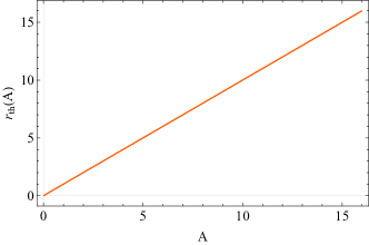
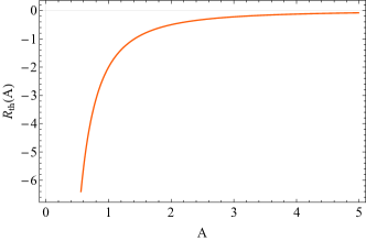
Figure 1: The wormhole throat $r_{\text{th}}(A)$ and the Ricci scalar $R_{\text{th}}(A)$ at the wormhole throat as a function of the scalar constant $A$, having set $c_{1}=-1$.

In FIG. 1 we plot the throat radius $r_{\text{th}}=m^{-1}=\sqrt{-A^{2}/c_{1}}$ as a function of $A$, where we can see their linear relation, having set $c_{1}=-1$. Wormholes exist only for negative $c_{1}$. To understand better what exactly happens at the throat of the wormhole, we also plot the Ricci scalar $R(r)$ at the throat as a function of the parameter $A$: $R_{r=r_{\text{th}}}(A)=-2m^{2}=2c_{1}/A^{2}$. A calculation of the Kretschmann scalar at the wormhole throat yields $K=12c_{1}^{2}/A^{4}$, which is in agreement with the behavior of the Ricci scalar. We can see that for larger $A$ the Ricci scalar gets weaker at the wormhole throat, so does the Kretschmann scalar. Thus, by increasing $A$ we obtain wormholes with larger throat radii which in turn decreases the curvature in the vicinity of the throat. Hence, $A$ affects the properties of our compact object in a similar manner with Ellis’s drainhole.

Additionally, we can perform a co-ordinate transformation to a chart $(t,l,\theta,\phi)$ where $l$ is the proper radial distance from the throat. In this chart the metric would be given by (6). Hence, by confronting the metrics (5) and (6) we can find the line element in this new coordinate system

$$ds^{2} = -Cdt^{2}+dl^{2}+r(l)^{2}d\Omega^{2}~{},$$ (39)

$$= -Cdt^{2}+dl^{2}+\left(\frac{e^{-lm}+e^{lm}}{2m}\right)^{2}d\Omega^{2}~{},$$ (40)

where, $r(l)=\cfrac{e^{-lm}+e^{lm}}{2m}=\cfrac{1}{m}\cosh(lm)$ and $l\in(-\infty,\infty)$ covering both sides of the wormhole.

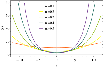
Figure 2: The function $r(l)$ for different values of the mass of the scalar field.

In FIG. 2 we can see the proper radial distance. The minimum represents the position of the wormhole throat.

III.3 Energy Conditions

Since we have obtained a wormhole configuration that satisfies the relative wormhole criteria we will briefly discuss the energy conditions and their violation. Therefore we recast Einstein equation (2) in the form

$$G_{\mu\nu}=T_{\mu\nu}^{grav}+f_{R}^{-1}T_{\mu\nu}^{\phi}=T_{\mu\nu}^{total}~{},$$ (41)

where, $T_{\mu\nu}^{grav}$ is given by

$$T_{\mu\nu}^{grav}=\frac{1}{2}g_{\mu\nu}\big{(}f_{R}^{-1}f(R)-R\big{)}-f_{R}^{-1}\big{(}g_{\mu\nu}\Box f_{R}-\nabla_{\mu}\nabla_{\nu}f_{R}\big{)}~{}$$ (42)

and can be regared as the effective stress energy tensor that non-linear gravity generates. Now, we switch to a set of orthonormal basis vectors, the proper reference frame where the basis vectors are expressed as [5]

$$e_{\hat{t}}=\exp(-\Phi)e_{t},\hskip 14.22636pte_{\hat{r}}=(1-b/r)^{1/2}e_{r},\hskip 14.22636pte_{\hat{\theta}}=r^{-1}e_{\theta},\hskip 14.22636pte_{\hat{\varphi}}=(r\sin\theta)^{-1}e_{\varphi}.$$ (43)

In this reference frame, we can identify, the energy density $\rho$, the radial pressure $p_{r}$ and the transverse pressure $p_{\theta,\varphi}$ in the following manner [75, 71]

$$\rho = G_{\hat{t}\hat{t}}=T_{\hat{t}\hat{t}}^{total}~{},$$ (44)

$$p_{r} = G_{\hat{r}\hat{r}}=T_{\hat{r}\hat{r}}^{total}~{},$$ (45)

$$p_{\theta,\varphi} = G_{\hat{\theta}\hat{\theta},\hat{\varphi}\hat{\varphi}}=T_{\hat{\theta}\hat{\theta},\hat{\varphi}\hat{\varphi}}^{total}~{}.$$ (46)

Now we will discuss the violation of the energy conditions [76]. The Weak Energy Condition (WEC) implies that any time like vector $x^{\mu}$ satisfies the condition

$$T_{\mu\nu}^{total}x^{\mu}x^{\nu}\geq 0~{}.$$ (47)

In the afforementioned reference frame this inequality takes the form

$$\rho>0~{}.$$ (48)

In our case we have

$$\rho=\frac{2}{r^{2}}-3m^{2}>0~{}.$$ (49)

The WEC is satisfied for any $m\neq 0$ and $0<r<\sqrt{\frac{2}{3m^{2}}}<\frac{1}{m}=r_{\text{th}}$. Therefore WEC is violated for any $r>r_{\text{th}}$.

The Null Energy Condition (NEC) states that

$$T_{\mu\nu}^{total}k^{\mu}k^{\nu}\geq 0~{},$$ (50)

for any null vector $k^{\mu}$. By continuity we expect that the WEC imples NEC. In the orthonormal frame the NEC reads

$$\rho+p_{r}\geq 0~{},$$ (51)

In our case NEC gives

$$\frac{2-3m^{2}r^{2}}{r^{2}}+m^{2}-\frac{2}{r^{2}}=-2m^{2}<0~{}.$$ (52)

Therefore NEC is always violated.

To have a better understanding on how the energy conditions are violated, we will discuss the energy conditions of the scalar field and the modified gravity part independently. For the scalar field we will only consider the $f_{R}^{-1}T^{\phi}_{\mu\nu}$ part of the energy momentum tensor in equation (41). In the afforementioned reference frame, we find that the energy density and the pressure are respectively

$$\rho^{\phi}=\frac{3}{r^{2}}~{},$$ (53)

$$p_{r}^{\phi}=\frac{3}{r^{2}}-6m^{2}~{}.$$ (54)

The WEC energy condition is satisfied for the scalar field while for the NEC we have that

$$\rho^{\phi}+p_{r}^{\phi}=\frac{6}{r^{2}}-6m^{2}>0~{},$$ (55)

which is satisfied for $r<\frac{1}{m}=r_{th}$ (outside of the wormhole region) and is violated outside and on the wormhole throat.

Now for the gravitational part of the energy momentum tensor we will only examine the $T_{\mu\nu}^{grav}$ term of (41). We find that the energy and pressure of the higher order gravity terms are respectively

$$\rho^{grav}=-3m^{2}-\frac{1}{r^{2}}~{},$$ (56)

$$p_{r}^{grav}=7m^{2}-\frac{5}{r^{2}}~{}.$$ (57)

The WEC is violated by the higher order gravity terms, while NEC yields

$$\rho^{grav}+p_{r}^{grav}=4m^{2}-\frac{6}{r^{2}}>0~{},$$ (58)

which holds for $r>\sqrt{\frac{3}{2}}\frac{1}{m}$ and is violated otherwise.

It is clear that if we add the energy densities of the matter and gravity part we obtain the total energy density (49) and the same happens with the pressures as expected. We note here that the modified gravity part of the action is responsible for the violation of WEC, while the NEC is violated by both matter and gravity for some range of the wormhole region $r\geq r_{th}=1/m$.

IV Conclusions

We studied wormhole solutions in a modified gravity theory in which the scalar curvature is generalized to a $f({\sf R})$ function. In this theory we considered a scalar field with negative kinetic energy, a phantom scalar field, with a self-interacting potential. Solving the field equations, choosing a function for the phantom scalar field, we find a wormhole solution without specifying the form of the $f({\sf R})$ function. The basic properties of this solution are that the presence of the phantom scalar field influences the scalar curvature and the size of the throat, and by increasing the strength of the scalar field we obtain wormholes with larger throat radii which in turn decreases the curvature in the vicinity of the throat.

Our obtained gravitational model satisfies the Dolgov-Kawasaki stability criterion, is tachyonically stable and it is free of ghosts. We calculated the NEC and the WEC and we showed that they are violated. We also investigated the matter and gravity part of the effective energy-momentum tensor independently to see their effects on the energy conditions. We found that the scalar filed respects WEC and violated NEC, while the gravity part of the effective energy-momentum tensor violates both WEC and NEC. We also note that the $f(\sf R)$ model we obtained resembles the Starobinsky inflation model [35].

Our solution cannot be reduced to GR. To do that we have to consider a more general metric ansatz such the one in [77] and try to find a solution to the $f({\sf R})$ field equations that reduces to the known solutions of GR [77, 78, 79]. In our work, the scalar field is minimally coupled to gravity via the volume element, so one could consider a more general ansatz like a regular non-minimally coupled scalar field that will violate the energy conditions and try to find wormhole solutions. It would also be interesting to check the stability of the obtained wormhole solution.

One can fix the $f({\sf R})$ function from the beginning and then look for wormhole solutions. For example in [56] a non-linear correction term in the scalar curvature was introduced $f({\sf R})=\sf R-2\alpha\sqrt{\sf R}$ where $\alpha$ has the dimensions of $|L|^{-1}$. In this modified gravity theory a new scale is introduced. Therefore to find a wormhole solution that resembles the original Ellis wormhole [20, 80] (or the $d$-dimensional generalization [81]) another scale has to be introduced to the theory to counterbalance the introduced gravitational scale. The easiest way to do that is to introduce a new scale via a self-interacting potential for the scalar field. So, one can consider our metric ansatz (5) and the Ellis scalar field (16) to find, at least in principle, a wormhole geometry, which will be reduced to the Ellis one, after parameterizing the constants of the solution appropriately. Wormholes with dynamical redshift function supported by a phantom scalar field might also be interesting to be studied.

- [1] L. Flamm, Phys. Z.17(1916) 448.
- [2] A. Einstein and N. Rosen, Phys. Rev.48(1935) 73.
- [3] C. W. Misner and J. A. Wheeler, Ann. Phys.2, 525 (1957); C. W. Misner, Phys. Rev.118, 1110 (1960).
- [4] J. A. Wheeler, Ann. Phys.2, 604 (1957);J. A. Wheeler, Geometrodynamics (Academic, New York, 1962).
- [5] M.S. Morris and K.S. Thorne, Am. J. Phys.56, 395 (1988); M. S. Morris, K. S. Thorne and U. Yurtsever,Phys. Rev. Lett.61, 1446 (1988).
- [6] V. Sahni and A. A. Starobinsky, Int. J. Mod. Phys. D09, 373 (2000); S. M. Carroll, Living Rev. Rel.4, 1 (2001); P. J. E. Peebles and B. Ratra, Rev. Mod. Phys.75, 559 (2003); P. F. Gonzales-Diaz, Phys. Rev. D65, 104035 (2002).
- [7] R. A. Konoplya and A. Zhidenko, ‘Traversable wormholes in General Relativity without exotic matter,” [arXiv:2106.05034 [gr-qc]].
- [8] E. Poisson and M. Visser, “Thin shell wormholes: Linearization stability,” Phys. Rev. D 52, 7318-7321 (1995) [arXiv:gr-qc/9506083 [gr-qc]].
- [9] L. A. Anchordoqui, S. E. Perez Bergliaffa and D. F. Torres, “Brans-Dicke wormholes in nonvacuum space-time,” Phys. Rev. D 55, 5226-5229 (1997) [arXiv:gr-qc/9610070 [gr-qc]]. A. G. Agnese and M. La Camera, “Wormholes in the Brans-Dicke theory of gravitation,” Phys. Rev. D 51, 2011-2013 (1995) K. K. Nandi, B. Bhattacharjee, S. M. K. Alam and J. Evans, “Brans-Dicke wormholes in the Jordan and Einstein frames,” Phys. Rev. D 57, 823-828 (1998) [arXiv:0906.0181 [gr-qc]]. A. Bhattacharya, I. Nigmatzyanov, R. Izmailov and K. K. Nandi, “Brans-Dicke Wormhole Revisited,” Class. Quant. Grav. 26, 235017 (2009) [arXiv:0910.1109 [gr-qc]]. K. K. Nandi, A. Islam and J. Evans, “Brans wormholes,” Phys. Rev. D 55, 2497-2500 (1997) [arXiv:0906.0436 [gr-qc]]; E. F. Eiroa, M. G. Richarte and C. Simeone, “Thin-shell wormholes in Brans-Dicke gravity,” Phys. Lett. A 373, 1-4 (2008) [erratum: Phys. Lett. 373, 2399-2400 (2009)] [arXiv:0809.1623 [gr-qc]]; F. S. N. Lobo and M. A. Oliveira, “General class of vacuum Brans-Dicke wormholes,” Phys. Rev. D 81, 067501 (2010) [arXiv:1001.0995 [gr-qc]]. S. V. Sushkov and S. M. Kozyrev, “Composite vacuum Brans-Dicke wormholes,” Phys. Rev. D 84, 124026 (2011) [arXiv:1109.2273 [gr-qc]]; E. Papantonopoulos and C. Vlachos, “Wormhole solutions in modified Brans-Dicke theory,” Phys. Rev. D 101, no.6, 064025 (2020) [arXiv:1912.04005 [gr-qc]].
- [10] R. Myrzakulov, L. Sebastiani, S. Vagnozzi and S. Zerbini, “Static spherically symmetric solutions in mimetic gravity: rotation curves and wormholes,” Class. Quant. Grav. 33, no.12, 125005 (2016) [arXiv:1510.02284 [gr-qc]].
- [11] M. G. Richarte and C. Simeone, “Wormholes in Einstein-Born-Infeld theory,” Phys. Rev. D 80, 104033 (2009) [erratum: Phys. Rev. D 81, 109903 (2010)] [arXiv:2006.12272 [gr-qc]]; N. M. Garcia and F. S. N. Lobo, “Wormhole geometries supported by a nonminimal curvature-matter coupling,” Phys. Rev. D 82, 104018 (2010) [arXiv:1007.3040 [gr-qc]]; N. Montelongo Garcia and F. S. N. Lobo, “Nonminimal curvature-matter coupled wormholes with matter satisfying the null energy condition,” Class. Quant. Grav. 28, 085018 (2011) [arXiv:1012.2443 [gr-qc]].
- [12] M. G. Richarte and C. Simeone, “Thin-shell wormholes supported by ordinary matter in Einstein-Gauss-Bonnet gravity,” Phys. Rev. D 76, 087502 (2007) [erratum: Phys. Rev. D 77, 089903 (2008)] [arXiv:0710.2041 [gr-qc]]; P. Kanti, B. Kleihaus and J. Kunz, “Wormholes in Dilatonic Einstein-Gauss-Bonnet Theory,” Phys. Rev. Lett. 107, 271101 (2011) [arXiv:1108.3003 [gr-qc]]; M. R. Mehdizadeh, M. Kord Zangeneh and F. S. N. Lobo, “Einstein-Gauss-Bonnet traversable wormholes satisfying the weak energy condition,” Phys. Rev. D 91, no.8, 084004 (2015) [arXiv:1501.04773 [gr-qc]]; M. Kord Zangeneh, F. S. N. Lobo and M. H. Dehghani, “Traversable wormholes satisfying the weak energy condition in third-order Lovelock gravity,” Phys. Rev. D 92, no.12, 124049 (2015) [arXiv:1510.07089 [gr-qc]]; G. Antoniou, A. Bakopoulos, P. Kanti, B. Kleihaus and J. Kunz, “Novel Einstein–scalar-Gauss-Bonnet wormholes without exotic matter,” Phys. Rev. D 101, no.2, 024033 (2020) [arXiv:1904.13091 [hep-th]]. B. Bhawal and S. Kar, “Lorentzian wormholes in Einstein-Gauss-Bonnet theory,” Phys. Rev. D 46, 2464-2468 (1992) H. Maeda and M. Nozawa, “Static and symmetric wormholes respecting energy conditions in Einstein-Gauss-Bonnet gravity,” Phys. Rev. D 78, 024005 (2008) [arXiv:0803.1704 [gr-qc]]. G. Dotti, J. Oliva and R. Troncoso, “Static wormhole solution for higher-dimensional gravity in vacuum,” Phys. Rev. D 75, 024002 (2007) [arXiv:hep-th/0607062 [hep-th]].
- [13] K. A. Bronnikov and A. M. Galiakhmetov, “Wormholes without exotic matter in Einstein–Cartan theory,” Grav. Cosmol. 21, no.4, 283-288 (2015) [arXiv:1508.01114 [gr-qc]]; K. A. Bronnikov and A. M. Galiakhmetov, “Wormholes and black universes without phantom fields in Einstein-Cartan theory,” Phys. Rev. D 94, no.12, 124006 (2016) [arXiv:1607.07791 [gr-qc]]; M. R. Mehdizadeh and A. H. Ziaie, “Dynamic wormhole solutions in Einstein-Cartan gravity,” Phys. Rev. D 96, no.12, 124017 (2017) [arXiv:1709.09028 [gr-qc]]; G. Kofinas, E. Papantonopoulos and E. N. Saridakis, “Self-Gravitating Spherically Symmetric Solutions in Scalar-Torsion Theories,” Phys. Rev. D 91, no.10, 104034 (2015) [arXiv:1501.00365 [gr-qc]]; I. P. Lobo, M. G. Richarte, J. P. Morais Graça and H. Moradpour, “Thin-shell wormholes in Rastall gravity,” Eur. Phys. J. Plus 135, no.7, 550 (2020) [arXiv:2007.05641 [gr-qc]].
- [14] J. M. Maldacena and L. Maoz, “Wormholes in AdS,” JHEP 02, 053 (2004) [arXiv:hep-th/0401024 [hep-th]].
- [15] R. V. Korolev and S. V. Sushkov, “Exact wormhole solutions with nonminimal kinetic coupling,” Phys. Rev. D 90, 124025 (2014) [arXiv:1408.1235 [gr-qc]].
- [16] R. Korolev, F. S. N. Lobo and S. V. Sushkov, “General constraints on Horndeski wormhole throats,” Phys. Rev. D 101, no.12, 124057 (2020) [arXiv:2004.12382 [gr-qc]].
- [17] R. Korolev, F. S. N. Lobo and S. V. Sushkov, “Kinetic gravity braiding wormhole geometries,” Phys. Rev. D 102, no.10, 104016 (2020) [arXiv:2009.04829 [gr-qc]].
- [18] C. Vlachos, E. Papantonopoulos and K. Destounis, “Echoes of Compact Objects in Scalar-Tensor Theories of Gravity,” Phys. Rev. D 103, no.4, 044042 (2021) [arXiv:2101.12196 [gr-qc]].
- [19] N. Chatzifotis, G. Koutsoumbas and E. Papantonopoulos, “Formation of bound states of scalar fields in AdS-asymptotic wormholes,” Phys. Rev. D 104, no.2, 024039 (2021) [arXiv:2011.08770 [gr-qc]].
- [20] H. G. Ellis, “Ether flow through a drainhole - a particle model in general relativity,” J. Math. Phys. 14, 104-118 (1973)
- [21] J. L. Blázquez-Salcedo, X. Y. Chew, J. Kunz and D. H. Yeom, “Ellis Wormholes in Anti-De Sitter Space,” [arXiv:2012.06213 [gr-qc]].
- [22] X. Y. Chew, B. Kleihaus and J. Kunz, “Geometry of Spinning Ellis Wormholes,” Phys. Rev. D 94, no.10, 104031 (2016) [arXiv:1608.05253 [gr-qc]].
- [23] X. Y. Chew, B. Kleihaus and J. Kunz, “Spinning Wormholes in Scalar-Tensor Theory,” Phys. Rev. D 97, no.6, 064026 (2018) [arXiv:1802.00365 [gr-qc]].
- [24] J. L. Blázquez-Salcedo, X. Y. Chew and J. Kunz, “Scalar and axial quasinormal modes of massive static phantom wormholes,” Phys. Rev. D 98, no.4, 044035 (2018) [arXiv:1806.03282 [gr-qc]].
- [25] P. K. Sahoo, P. H. R. S. Moraes, P. Sahoo and G. Ribeiro, “Phantom fluid supporting traversable wormholes in alternative gravity with extra material terms,” Int. J. Mod. Phys. D 27, no.16, 1950004 (2018) [arXiv:1802.02465 [gr-qc]].
- [26] P. Goulart, “Phantom wormholes in Einstein–Maxwell-dilaton theory,” Class. Quant. Grav. 35, no.2, 025012 (2018) [arXiv:1708.00935 [gr-qc]].
- [27] A. De Felice and S. Tsujikawa, “f(R) theories,” Living Rev. Rel. 13, 3 (2010) [arXiv:1002.4928 [gr-qc]].
- [28] G. Cognola, E. Elizalde, S. Nojiri, S. D. Odintsov, L. Sebastiani and S. Zerbini, “A Class of viable modified f(R) gravities describing inflation and the onset of accelerated expansion,” Phys. Rev. D 77 (2008) 046009 [arXiv:0712.4017 [hep-th]].
- [29] P. Zhang, “Testing gravity against the large scale structure of the universe.,” Phys. Rev. D 73 (2006) 123504 [astro-ph/0511218].
- [30] B. Li and J. D. Barrow, “The Cosmology of f(R) gravity in metric variational approach,” Phys. Rev. D 75 (2007) 084010 [gr-qc/0701111].
- [31] Y. S. Song, H. Peiris and W. Hu, “Cosmological Constraints on f(R) Acceleration Models,” Phys. Rev. D 76 (2007) 063517 [arXiv:0706.2399 [astro-ph]].
- [32] S. Nojiri and S. D. Odintsov, “Modified f(R) gravity unifying R**m inflation with Lambda CDM epoch,” Phys. Rev. D 77 (2008) 026007 [arXiv:0710.1738 [hep-th]].
- [33] S. Nojiri and S. D. Odintsov, “Unifying inflation with LambdaCDM epoch in modified f(R) gravity consistent with Solar System tests,” Phys. Lett. B 657 (2007) 238 [arXiv:0707.1941 [hep-th]].
- [34] S. Capozziello, C. A. Mantica and L. G. Molinari, “Cosmological perfect-fluids in f(R) gravity,” Int. J. Geom. Meth. Mod. Phys. 16 (2018) no.01, 1950008 [arXiv:1810.03204 [gr-qc]].
- [35] A. A. Starobinsky, “A New Type of Isotropic Cosmological Models Without Singularity,” Phys. Lett. B 91 (1980) 99 [Phys. Lett. 91B (1980) 99] [Adv. Ser. Astrophys. Cosmol. 3 (1987) 130].
- [36] S. Capozziello, O. Farooq, O. Luongo and B. Ratra, “Cosmographic bounds on the cosmological deceleration-acceleration transition redshift in gravity,” Phys. Rev. D 90, no.4, 044016 (2014) [arXiv:1403.1421 [gr-qc]].
- [37] M. Ostrogradsky, “Mémoires sur les équations différentielles, relatives au problème des isopérimètres,” Mem. Acad. St. Petersbourg 6 (1850) no.4, 385.
- [38] R. P. Woodard, “Avoiding dark energy with 1/r modifications of gravity,” Lect. Notes Phys. 720 (2007) 403 [astro-ph/0601672].
- [39] L. Sebastiani and S. Zerbini, “Static Spherically Symmetric Solutions in F(R) Gravity,” Eur. Phys. J. C 71, 1591 (2011) [arXiv:1012.5230 [gr-qc]].
- [40] T. Multamaki and I. Vilja, “Spherically symmetric solutions of modified field equations in f(R) theories of gravity,” Phys. Rev. D 74, 064022 (2006) [arXiv:astro-ph/0606373 [astro-ph]].
- [41] S. H. Hendi, “(2+1)-Dimensional Solutions in Gravity,” Int. J. Theor. Phys. 53, no.12, 4170-4181 (2014) [arXiv:1410.7527 [gr-qc]].
- [42] S. H. Hendi, B. Eslam Panah and R. Saffari, “Exact solutions of three-dimensional black holes: Einstein gravity versus gravity,” Int. J. Mod. Phys. D 23, no.11, 1450088 (2014) [arXiv:1408.5570 [hep-th]].
- [43] T. Multamaki and I. Vilja, “Static spherically symmetric perfect fluid solutions in f(R) theories of gravity,” Phys. Rev. D 76, 064021 (2007) [arXiv:astro-ph/0612775 [astro-ph]].
- [44] G. G. L. Nashed and E. N. Saridakis, “New rotating black holes in nonlinear Maxwell gravity,” Phys. Rev. D 102, no.12, 124072 (2020) [arXiv:2010.10422 [gr-qc]].
- [45] G. G. L. Nashed and S. Nojiri, “Analytic charged BHs in f(R) gravity,” Phys. Lett. B 820, 136475 (2021) [arXiv:2010.04701 [hep-th]].
- [46] G. G. L. Nashed and K. Bamba, “Charged spherically symmetric Taub–NUT black hole solutions in gravity,” PTEP 2020, no.4, 043E05 (2020) [arXiv:1902.08020 [gr-qc]].
- [47] G. G. L. Nashed and S. Capozziello, “Charged spherically symmetric black holes in gravity and their stability analysis,” Phys. Rev. D 99, no.10, 104018 (2019) [arXiv:1902.06783 [gr-qc]].
- [48] J. A. R. Cembranos, A. de la Cruz-Dombriz and P. Jimeno Romero, “Kerr-Newman black holes in theories,” Int. J. Geom. Meth. Mod. Phys. 11 (2014) 1450001 [arXiv:1109.4519 [gr-qc]].
- [49] A. de la Cruz-Dombriz, A. Dobado and A. L. Maroto, “Black Holes in f(R) theories,” Phys. Rev. D 80 (2009) 124011 Erratum: [Phys. Rev. D 83 (2011) 029903] [arXiv:0907.3872 [gr-qc]].
- [50] S. C. Jaryal and A. Chatterjee, “Gravitationally collapsing stars in gravity,” Eur. Phys. J. C 81, no.4, 273 (2021) [arXiv:2102.08717 [gr-qc]].
- [51] S. H. Hendi, B. Eslam Panah and S. M. Mousavi, “Some exact solutions of F(R) gravity with charged (a)dS black hole interpretation,” Gen. Rel. Grav. 44, 835 (2012) [arXiv:1102.0089 [hep-th]].
- [52] E. F. Eiroa and G. Figueroa-Aguirre, “Thin shells in ( 2+1 )-dimensional gravity,” Phys. Rev. D 103, no.4, 044011 (2021) [arXiv:2011.14952 [gr-qc]].
- [53] Z. Y. Tang, B. Wang and E. Papantonopoulos, “Exact charged black hole solutions in -dimensions in gravity,” Eur. Phys. J. C 81, no.4, 346 (2021) [arXiv:1911.06988 [gr-qc]].
- [54] Z. Y. Tang, B. Wang, T. Karakasis and E. Papantonopoulos, “Curvature scalarization of black holes in f(R) gravity,” Phys. Rev. D 104, no.6, 064017 (2021) [arXiv:2008.13318 [gr-qc]].
- [55] T. Karakasis, E. Papantonopoulos, Z. Y. Tang and B. Wang, “Black holes of (2+1)-dimensional gravity coupled to a scalar field,” Phys. Rev. D 103, no.6, 064063 (2021) [arXiv:2101.06410 [gr-qc]].
- [56] T. Karakasis, E. Papantonopoulos, Z. Y. Tang and B. Wang, “Exact Black Hole Solutions with a Conformally Coupled Scalar Field and Dynamic Ricci Curvature in Gravity Theories,” Eur. Phys. J. C 81, 897 (2021) [arXiv:2103.14141 [gr-qc]].
- [57] S. Pi, Y. l. Zhang, Q. G. Huang and M. Sasaki, “Scalaron from -gravity as a heavy field,” JCAP 05, 042 (2018) [arXiv:1712.09896 [astro-ph.CO]].
- [58] A. de la Cruz-Dombriz, E. Elizalde, S. D. Odintsov and D. Sáez-Gómez, “Spotting deviations from R2 inflation,” JCAP 05, 060 (2016) [arXiv:1603.05537 [gr-qc]].
- [59] F. S. N. Lobo and M. A. Oliveira, “Wormhole geometries in f(R) modified theories of gravity,” Phys. Rev. D 80, 104012 (2009) [arXiv:0909.5539 [gr-qc]].
- [60] C. Bejarano, E. F. Eiroa and G. Figueroa-Aguirre, “Thin-shell wormholes in (2+1)-dimensional F(R) theories,” Eur. Phys. J. C 81, 668 (2021) [arXiv:2103.16482 [gr-qc]].
- [61] E. F. Eiroa and G. Figueroa Aguirre, “Thin-shell wormholes with charge in F(R) gravity,” Eur. Phys. J. C 76, no.3, 132 (2016) [arXiv:1511.02806 [gr-qc]].
- [62] E. F. Eiroa and G. Figueroa Aguirre, “Thin-shell wormholes with a double layer in quadratic F(R) gravity,” Phys. Rev. D 94, no.4, 044016 (2016) [arXiv:1605.07089 [gr-qc]].
- [63] M. F. Shamir and I. Fayyaz, “Traversable wormhole solutions in gravity via Karmarkar condition,” Eur. Phys. J. C 80, no.12, 1102 (2020) [arXiv:2012.02582 [gr-qc]].
- [64] S. V. Chervon, J. C. Fabris and I. V. Fomin, “Black holes and wormholes in gravity with a kinetic curvature scalar,” Class. Quant. Grav. 38, no.11, 115005 (2021) [arXiv:2008.12143 [gr-qc]].
- [65] N. Godani and G. C. Samanta, “Traversable wormholes in gravity with constant and variable redshift functions,” New Astron. 80, 101399 (2020) [arXiv:2004.14209 [gr-qc]].
- [66] T. Tangphati, A. Chatrabhuti, D. Samart and P. Channuie, “Traversable wormholes in -massive gravity,” Phys. Rev. D 102, no.8, 084026 (2020) [arXiv:2003.01544 [gr-qc]].
- [67] J. L. Rosa, J. P. S. Lemos and F. S. N. Lobo, “Wormholes in generalized hybrid metric-Palatini gravity obeying the matter null energy condition everywhere,” Phys. Rev. D 98, no.6, 064054 (2018) [arXiv:1808.08975 [gr-qc]].
- [68] P. Cañate, “A no-hair theorem for black holes in gravity,” Class. Quant. Grav. 35, no.2, 025018 (2018).
- [69] J. Sultana and D. Kazanas, “A no-hair theorem for spherically symmetric black holes in gravity,” Gen. Rel. Grav. 50, no.11, 137 (2018) [arXiv:1810.02915 [gr-qc]].
- [70] P. Cañate, L. G. Jaime and M. Salgado, “Spherically symmetric black holes in gravity: Is geometric scalar hair supported ?,” Class. Quant. Grav. 33, no.15, 155005 (2016) [arXiv:1509.01664 [gr-qc]].
- [71] M. Visser, “Lorentzian wormholes: From Einstein to Hawking,” Woodbury, USA: AIP (1995) 412 p.
- [72] V. Faraoni, “Matter instability in modified gravity,” Phys. Rev. D 74, 104017 (2006) [arXiv:astro-ph/0610734 [astro-ph]].
- [73] V. Faraoni, “f(R) gravity: Successes and challenges,” [arXiv:0810.2602 [gr-qc]].
- [74] O. Bertolami and M. C. Sequeira, “Energy Conditions and Stability in f(R) theories of gravity with non-minimal coupling to matter,” Phys. Rev. D 79, 104010 (2009) [arXiv:0903.4540 [gr-qc]].
- [75] M. Visser, S. Kar and N. Dadhich, “Traversable wormholes with arbitrarily small energy condition violations,” Phys. Rev. Lett. 90, 201102 (2003) [arXiv:gr-qc/0301003 [gr-qc]].
- [76] F. Rahaman, M. Kalam and S. Chakraborty, “Thin shell wormholes in higher dimensiaonal Einstein-Maxwell theory,” Gen. Rel. Grav. 38, 1687-1695 (2006) [arXiv:gr-qc/0607061 [gr-qc]].
- [77] K. A. Bronnikov, “Scalar fields as sources for wormholes and regular black holes,” Particles 1, no.1, 56-81 (2018) [arXiv:1802.00098 [gr-qc]].
- [78] H. Huang, H. Lü and J. Yang, “Bronnikov-like Wormholes in Einstein-Scalar Gravity,” [arXiv:2010.00197 [gr-qc]].
- [79] H. Huang and J. Yang, “Charged Ellis Wormhole and Black Bounce,” Phys. Rev. D 100, no.12, 124063 (2019) [arXiv:1909.04603 [gr-qc]].
- [80] P. Cañate, J. Sultana and D. Kazanas, “Ellis wormhole without a phantom scalar field,” Phys. Rev. D 100, no.6, 064007 (2019) [arXiv:1907.09463 [gr-qc]].
- [81] F. Rahaman, M. Kalam and K. A. Rahman, “Wormholes supported by Scalar Fields with Negative Kinetic Energy,” Int. J. Mod. Phys. A 24, 5007-5018 (2009) [arXiv:0811.2657 [gr-qc]].