Integral decomposition for the solutions of the generalized Cattaneo equation

Abstract

We present the integral decomposition for the fundamental solution of the generalized Cattaneo equation with both time derivatives smeared through convoluting them with some memory kernels. For power-law kernels $t^{-\alpha}$, $\alpha\in(0,1]$ this equation becomes the time fractional one governed by the Caputo derivatives which highest order is 2. To invert the solutions from the Fourier-Laplace domain to the space-time domain we use analytic methods based on the Efross theorem and find out that solutions looked for are represented by integral decompositions which tangle the fundamental solution of the standard Cattaneo equation with non-negative and normalizable functions being uniquely dependent on the memory kernels. Furthermore, the use of methodology arising from the theory of complete Bernstein functions allows us to assign such constructed integral decompositions the interpretation of subordination. This fact is preserved in two limit cases built into the generalized Cattaneo equations, i.e., either the diffusion or the wave equations. We point out that applying the Efross theorem enables us to go beyond the standard approach which usually leads to the integral decompositions involving the Gaussian distribution describing the Brownian motion. Our approach clarifies puzzling situation which takes place for the power-law kernels $t^{-\alpha}$ for which the subordination based on the Brownian motion does not work if $\alpha\in(1/2,1]$.

I Introduction

Diffusion influences the course of kinetic phenomena investigated in many branches of pure physics, chemistry, and biology but its applications are by no means restricted to the fundamental problems of Nature. Knowledge of the origin and effects of diffusion mechanisms is necessary to understand diversity of results obtained in life, earth and environment sciences as well as in materials engineering and technological processes. Diffusion governs behaviour of phenomena occurring both in simple and complex systems, from the Brownian motion discussed in the course of the school physics to very special and advanced problems, like the transport phenomena in tissues and cells dif1 ; JHJeon11 ; JFReverey15 , spreading infectious diseases and drug administration dif2 , using zeolites in catalysis dif3 , environmental science dif4 , materials engineering and manufacturing new materials dif5 ; diff5a , and even finances diff5b . Comprehensive information on a diffusion process under study is not easy to get. Usually it strongly depends on the properties of the system under consideration and routinely its quantitive analyses start from determining the relation between the time $t$ and the mean square displacement (MSD) $\langle x^{2}(t)\rangle$ of diffusing objects. For the case of Brownian motion it takes the form of the Einstein-Smoluchowski relation $\langle x^{2}(t)\rangle\propto t$. The latter is valid for any $t\in\mathbb{R}_{+}$ and besides of the Brownian motion characterizes also other transport processes classified, in general, as the normal diffusion. Processes which exhibit deviations from the Einstein-Smoluchowski relation, e.g., lead to the relation $\langle x^{2}(t)\rangle\propto t^{\mu},\mu>0$ (valid at least asymptotically for small and/or large time) JWHaus87 ; RMetzler14 ; RMetzler19 , are classified as the anomalous diffusion and are nick-named the sub- and superdiffusion in dependence of the value of $\mu$. For $\mu\in(0,1)$ we deal with the subdiffusion whereas the cases $\mu>1$ are called the superdiffusion. If $\mu=2$ then the process bears the special name of ballistic motion. Here it has to be noted that contrary to the Einstein-Smoluchowski relation supposed to be satisfied for all admissible range of time there exist experimentally observed relations between $\langle x^{2}(t)\rangle$ and $t$ which change their functional shape as the time flows on. Retrieving such information provides us with some hints how to choose the type of evolution equation suitable to describe correctly the process under investigation. Well-researched approach is to modify the standard diffusion equation into its fractional counterpart

$$\partial_{t}p(x,t)=B\partial_{x}^{2}p(x,t)\longrightarrow{{}_{c}D}^{\mu}_{t}p(x,t)=B\partial_{x}^{2}p(x,t),$$ (1)

with ${{}_{c}D}^{\mu}_{t}$ being the (Caputo) fractional time derivative of the order $\mu$, which leads to $\langle x^{2}(t)\rangle\propto t^{\mu}$. This simple modification is not enough if the behavior of MSD changes its shape with time - in such a case one has to go beyond Eq. (1) and consider more complicated evolution equations like the standard or fractional Cattaneo equations comprising more than one time derivative term and possibly involving more general forms of the time smearing than the standard fractional derivatives do. Adequate example have been studied recently in KGorska20 and reads

$$\tau\int_{0}^{t}\eta(t-\xi)\partial_{\xi}^{2}q_{\hat{\gamma}}(\tau;x,\xi)\operatorname{d\!}\xi+\int_{0}^{t}\gamma(t-\xi)\partial_{\xi}q_{\hat{\gamma}}(\tau;x,\xi)\operatorname{d\!}\xi\\ =B\,\partial_{x}^{2}q_{\hat{\gamma}}(\tau;x,t)$$ (2)

where $B$ is the diffusion coefficient. In what follows the subscript ’$\hat{\gamma}$’ is used to emphasize the role played by the Laplace transformed function $\gamma(t)$, namely $\hat{\gamma}(z)=\mathcal{L}[\gamma(t);z]$. The solution $q_{\hat{\gamma}}(\tau;x,t)$, if it is to be interpreted as the probability density (PDF) of finding the particle in a position $x\in\mathbb{R}$ at an instant of time $t>0$, must be shown non-negative and normalizable for chosen memory functions $\eta(t)$ and $\gamma(t)$. The memory functions $\eta(t)$ and $\gamma(t)$ express the smearing of the second and first time derivatives, respectively, and for special choices reduce Eq. (2) to more familiar cases: for $\eta(t)=0$ Eq. (2) becomes the time smeared diffusion equation

$$\int_{0}^{t}\gamma(t-\xi)\partial_{\xi}N_{\hat{\gamma}}(x,\xi)\operatorname{d\!}\xi=B\,\partial_{x}^{2}N_{\hat{\gamma}}(x,t)$$ (3)

while for $\gamma(t)=\eta(t)=\delta(t)$, with $\delta(t)$ being the Dirac distribution, Eq. (2) is the standard Cattaneo equation CRCattaneo48 ; CRCattaneo58 . The striking feature of the latter is that its fundamental solution (i.e. evolution of the space localized time initial condition), similarly to the case of wave equation, does vanish outside the compact support $\Delta(x,t)\in\mathbb{R}\otimes\mathbb{R}_{+}$ JAStratton41 ; PMMorse53 ; JMasoliver96 . Thus it appears justified to ask if already mentioned properties, i.e., the functional dependence on $t$ which MSD obeys in $t$ and the compact character of $\Delta(x,t)$ are kept for the time smeared Cattaneo equation Eq. (2). To judge the problem we shall consider the power-law memory functions being the most frequently used type of functions adopted to mimic the memory effects.

Looking for the answer to the above questions let us note that Eqs. (2) and (3) differ only by the term containing the parameter $\tau$. For small $\tau$ Eq. (2) formally tends to Eq. (3), i.e., to the time smeared diffusion equation. On the opposite, for large $\tau$, the smeared second time derivative dominates and we can neglect the smeared first time derivative. So we arrive at the so-called time-smeared diffusion-wave equation which, if detailed to the fractional derivative case, was studied in TSandev18 ; YuLuchko13 ; YuLuchko19 . Hence, Eq. (2), with $\tau$ treated as a free parameter, describes all intermediate cases. This feature should be also reflected in the limit behaviour of $q_{\hat{\gamma}}(\tau;x,t)$:

$$N_{\hat{\gamma}}(x,t)=\lim_{\tau\to 0}q_{\hat{\gamma}}(\tau;x, t)\quad\text{and}$$ (4)

$$W_{\hat{\gamma}}(x,t)=\lim_{\tau\to\infty}q_{\hat{\gamma}}(\tau;x,t),$$ (5)

where in the shorthand notation these two limits will be marked as $q_{\hat{\gamma}}(0;x,t)$ and $q_{\hat{\gamma}}(\infty;x,t)$.

The solutions $N_{\hat{\gamma}}(x,t)$ and $W_{\hat{\gamma}}(x,t)$ can be represented in the form of integral decomposition introduced in Ref. HCFogedby94 . The characteristic property of such a formalism is that one replaces their physically observed dependence on the space coordinate $x$ and the physical (laboratory) time coordinate $t$ by the braided distributions of the space coordinate $x$ evolving according to an internal (operational) time $\xi$ which, in turn, is assumed to be stochastically dependent on the clock measured laboratory time $t$. Integral decomposition entwines both distributions, threated as independent, through the integral taken over internal, or operational, time $\xi$. From the widely known results, e.g, IMSokolov02 ; IMSokolov05 ; ABaule03 ; AChechkin21 , we learn that $N_{\hat{\gamma}}(x,t)$ can be given by

$$N_{\hat{\gamma}}(x,t)=\int_{0}^{\infty}N(x,\xi)f_{0}(\xi,t)\operatorname{d\!}\xi,$$ (6)

where

$$N(x,t)=\operatorname{e}^{-x^{2}/(4Bt)}/\sqrt{4\pi Bt}$$ (7)

and

$$f_{0}(\xi,t)=\mathcal{L}^{-1}[\hat{\gamma}(z)\operatorname{e}^{-\xi z\hat{\gamma}(z)};t].$$ (8)

As presented in (TSandev18, , Eq. (11)) for the case of the wave-diffusion equation and its solution $W_{\hat{\gamma}}(x,t)$ the integral decomposition has the form of Eq. (6) but instead of $f_{0}(\xi,t)$ one has

$$f_{\infty}(\xi,t)=\mathcal{L}^{-1}\{z\hat{\eta}(z)\exp[-\xi z^{2}\hat{\eta}(z)];t\}.$$ (9)

Note that subscripts ’$0$’ and ’$\infty$’ in Eqs. (8) and (9) are used in the context of previously discussed limits of the generalized Cattaneo equation. Within the investigation of diffusion phenomena rooted in the stochastic processes approach it is said that $f_{0}(\xi,t)$ or $f_{\infty}(\xi,t)$ subordinate the normal distribution if all functions involved in the game: $N(x,\xi)$, $f_{0}(\xi,t)$ and $f_{\infty}(\xi,t)$ are independent PDFs given by non-negative, normalized, and infinitely divisible functions. These conditions are satisfied by the normal distribution $N(x,t)$. Nevertheless, the problem arises with the functions $f_{0}(\xi,t)$ and $f_{\infty}(\xi,t)$ which may or may not obey all these conditions. Consequently, it is needed to distinguish two classes of $f_{..}(\cdot,-)$’s - if they are independent PDFs satisfying all just mentioned requirements then due to IMSokolov02 ; AChechkin21 are named “safe” functions; in the opposite case they are called “dangerous”. Besides of being independent on $N(x,\xi)$ the sufficient condition for the functions $f_{0}(\xi,t)$ and $f_{\infty}(\xi,t)$ to be the “safe” ones is fulfilled if $z\hat{\gamma}(z)$ or $z^{2}\hat{\eta}(z)$ belong, for $z$ restricted to $\mathbb{R}_{+}$, to the class of the so-called completely Bernstein functions (CBF) which definition is quoted in the Appendix A. Concluding this part of our considerations: usage of subordination approach works correctly if $f_{0}(\xi,t)$ or $f_{\infty}(\xi,t)$, respectively, are PDFs independent on $N(x,\xi)$ and are given by the completely Bernstein functions. It is important to fully clarify the problem because subordination is the cornerstone of the stochastic processes framework and is based on introducing the operational time $\xi(t)$. The later in fact the operational time means a time-like parametrization of the composite (parent) process $X(\xi(t))$ given by the Brownian motion with jumps stochastically distributed in the operational time $\xi(t)$.

Throughout the paper we use the relation between memories $\eta(t)$ and $\gamma(t)$ which comes out, as a constraint, from consistency conditions put on the smearing of the first and second time derivatives. These relations have been derived in KGorska20 and according to them if the memory function $\gamma(t)$ is made responsible for the time smearing of the first time derivative then

$$\eta(t)=\int_{0}^{t}\gamma(\xi)\gamma(t-\xi)\operatorname{d\!}\xi,\qquad\hat{\eta}(z)=\hat{\gamma}^{2}(z)$$ (10)

represents the smearing of the second time derivative. Authors of many theoretical and experimental studies concerning termoelasticity YZPovstenko15 , anomalous transport in complex media ACompte97 ; EAwad20 ; AGiusti18 , chemical reactions TKosztolowicz14 ; KDLewandowska08 are used to model the memory functions by the power-law functions $\eta(t)\propto t^{1-2\alpha}$ and $\gamma(t)\propto t^{-\alpha}$, $\alpha\in(0,1]$ which in the Laplace domain read $\hat{\eta}(z)=z^{2(\alpha-1)}$ and $\hat{\gamma}(z)=z^{\alpha-1}$. In such a case $f_{0}(\xi,t)$ is always “safe”, i.e., correctly defined PDF but, as shown in Ref. TSandev18 , $f_{\infty}(\xi,t)$ is not “safe” PDF for $\alpha\in(1/2,1]$. Thus, for $\alpha\in(1/2,1]$, the integral decomposition of the fundamental solution to the generalized Cattaneo equation based on the normal distribution must not be treated any longer as a subordination. From the other side, as shown in Ref. KGorska20 , this solution is non-negative and normalizable. In what follows we will present the solution to this puzzle and propose an alternative integral decomposition which keeps $f_{0}(\xi,t)$ but instead of $N(x,\xi)$ it involves the fundamental solution of the Cattaneo equation if $\alpha\in(1/2,1]$.

The paper is organized as follows. In Sec. II we study two ways to obtain the integral decompositions suitable for the generalized Cattaneo equation. Following the first, usually adopted, one we arrive at the product of the normal distribution and the function which is not always “safe” PDF. Within the alternative approach the use of Efross theorem allows one to find integral decomposition in which the normal distribution is replaced by the solution of the standard Cattaneo equation. We show that in such a case we get the integral which integrand is the product of functions being “safe” PDFs. Thus, our integral decomposition expresses the subordination approach. In Sec. III, taking the appropriate limit of $\tau$, we present the passage from the integral decomposition introduced in the paper into the known examples of integral decomposition got for the solutions of the anomalous diffusion and diffusion-wave equations. In Sec. IV our construction of integral decompositions is illustrated on three examples characterized by important role played by the memory effects - either the strictly localized case or the power-law memory functions or mixture of these two. Results of the paper are resumed and discussed in Sec. V while Sec. VI contains concluding remarks concerning prospective applications of the Efross theorem based integral decompositions used as a tool to investigate both some fundamental problems as well as hot topics recently emerging in the anomalous diffusion. The paper is completed by five appendixes devoted to explanation of mathematics used throughout the text.

II Integral decomposition

It is an obvious statement that any integral decomposition relied on factorization of the space and time coordinates is not unique. Using integral decompositions to describe anomalous diffusion and non-Debye relaxations is commonly justified by physical and mathematical considerations based on modeling these phenomena by stochastic processes underlying them AStanislavsky17 ; AStanislavsky19 . Integral decompositions represent joint probabilities and provide us with the correct answer if the integrals under study are not only non-negative and normalizable on $\mathbb{R}_{+}$ but also result from composition of infinitely divisible distributions AChechkin21 ; Bochner . Namely this condition allows to equip them with probabilistic interpretation and to use methods elaborated within the theory of stochastic processes, among them the subordination approach AChechkin21 ; Bochner . In what follows we shall show how to construct, without recalling probabilistic tools, integral decompositions which represent non-negative normalizable solutions to diffusion equations of the type Eq. (2).

II.1 Integral decomposition preserving the $N(x,\xi)$ distribution

Eq. (6) with Eqs. (8) or (9) put in are special cases of the solution to Eq. (2). In the Fourier-Laplace domain it reads

$$\hat{\tilde{q}}_{\hat{\gamma}}(\tau;k,z)=\frac{z^{-1}\hat{M}_{\hat{\gamma}}(z)}{\hat{M}_{\hat{\gamma}}(z)+Bk^{2}},$$ (11)

where

$$\hat{M}_{\hat{\gamma}}(z)=\tau[z\hat{\gamma}(z)]^{2}+z\hat{\gamma}(z).$$ (12)

The symbols ’$\sim$’ and $k$ are related to the Fourier transform whereas ’$\wedge$’ and $z$ correspond to the Laplace transform. Using $b^{-1}=\int_{0}^{\infty}\exp(-b\xi)\operatorname{d\!}\xi$ to get rid of the denominator in Eq. (11) we are able to rewrite Eq. (11) as

$$\hat{\tilde{q}}_{\hat{\gamma}}(\tau;k,z)=\int_{0}^{\infty}\operatorname{e}^{-\xi Bk^{2}}\,z^{-1}\hat{M}_{\hat{\gamma}}(z)\operatorname{e}^{-\xi\hat{M}_{\hat{\gamma}}(z)}\operatorname{d\!}\xi.$$ (13)

The term $\exp(-\xi Bk^{2})$ corresponds, by the inverse Fourier transform, to the normal distribution $N(x,\xi)$, whereas taking the inverse Laplace transform of the $z$ dependent term we get

$$q_{\hat{\gamma}}(\tau;x,t)=\int_{0}^{\infty}N(x,\xi)\,f_{\tau}(\xi,t)\operatorname{d\!}\xi$$ (14)

where

$$f_{\tau}(\xi,t)=\mathcal{L}^{-1}[z^{-1}\hat{M}_{\hat{\gamma}}(z)\operatorname{e}^{-\xi\hat{M}_{\hat{\gamma}}(z)};t].$$ (15)

The function $f_{\tau}(\xi,t)$ tends to $f_{0}(\xi,t)$ for $\tau\to 0$ and to $f_{\infty}(\xi,t)$ for $\tau\to\infty$. To show that $f_{\tau}(\xi,t)$ is “safe” PDF means to prove that it is normalized, non-negative, and infinitely divisible. Normalizability is easily seen, $\int_{0}^{\infty}f_{\tau}(\xi,t)\operatorname{d\!}\xi=\mathcal{L}^{-1}[z^{-1};t]=1$. Non-negativity of $f_{\tau}(\xi,t)$ comes out from the Bernstein theorem presented in Appendix A. Due to this theorem $f_{\tau}(\xi,t)$ is non-negative if $z^{-1}\hat{M}_{\hat{\gamma}}(z)\exp[-\xi\hat{M}_{\hat{\gamma}}(z)]$, $z\in\mathbb{R}_{+}$, is given by a completely monotone function (CMF), i.e. non-negative function whose all derivatives exist on $\mathbb{R}_{+}$ and alternate RLSchilling10 . Because the product of CMFs is CMF then the Laplace transform of $f_{\tau}(\xi,t)$ is CMF if $z^{-1}\hat{M}_{\hat{\gamma}}(z)$ and $\exp[-\xi\hat{M}_{\hat{\gamma}}(z)]$ are CMFs. Both of these conditions are ensured for $\hat{M}_{\hat{\gamma}}(z)$ being CBF. The completely Bernstein character of $\hat{M}_{\hat{\gamma}}(z)$ guarantees also that $f_{\tau}(\xi,t)$ is an infinitely divisible distribution, see Appendix B. Thus, we end up with the conclusion that if $\hat{M}_{\hat{\gamma}}(z)$ is CBF then $f_{\tau}(\xi,t)$ is infinitely divisible PDF so it may be claimed that it subordinates $N(x,\xi)$.

Let us check if the above statement appears conclusive for some special cases of Eq. (2). For the standard Cattaneo equation with $\hat{\eta}(z)=\hat{\gamma}(z)=1$ we have $\hat{M}_{1}(z)=\tau z^{2}+z$ which is not CBF. So the appropriate $f_{\tau}(\xi,t)$ in not PDF and it does not subordinate $N(x,\xi)$. As the next example we take Eq. (2) with the power-law memory functions. Now $\hat{M}_{\hat{\gamma}}(z)=\tau z^{2\alpha}+z^{\alpha}$ is CBF only if $\alpha\in(0,1/2]$ whereas for the remaining values of $\alpha$, that is $\alpha\in(1/2,1]$, it is not CBF. It means that for this example $f_{\tau}(\xi,t)$ is a “safe” PDF only for $\alpha\in(0,1/2]$ and it is “dangerous” if $\alpha\in(1/2,1]$. Thus, it exhibits the behavior of $f_{\infty}(\xi,t)$ presented in TSandev18 .

The above examples show that the integral decomposition given by Eq. (14) must not be always treated as the subordination of two processes. We shall propose another type integral decomposition within which, still keeping $f_{0}(\xi,t)$ present, we will use another parent process instead of Gaussian distribution characteristic for the Brownian motion.

II.2 Integral decomposition preserving $f_{0}(\xi,t)$

To obtain the integral decomposition different than Eq. (14) we first calculate the Fourier transform of Eq. (11). That gives

$$\hat{q}_{\hat{\gamma}}(\tau;x,z)=\frac{z^{-1}[\hat{M}_{\hat{\gamma}}(z)]^{1/2}}{2\sqrt{B}}\exp\Big{\{}-\frac{|x|}{\sqrt{B}}[\hat{M}_{\hat{\gamma}}(z)]^{1/2}\Big{\}},$$ (16)

which can be rewritten as

$$\hat{q}_{\hat{\gamma}}(\tau;x,z)=\hat{\gamma}(z)F(x,g(z)),$$ (17)

where

$$F(x,g)=\frac{1}{2a}\frac{1/(2\tau)+g}{\sqrt{g^{2}-1/(4\tau^{2})}}\operatorname{e}^{-\frac{|x|}{a}\sqrt{g^{2}-1/(4\tau^{2})}}$$ (18)

and $g$ is a shorthand of $g(z)$ for simplifying the notation. The non-negative constant $a$ is equal to $(B/\tau)^{1/2}$ while the auxiliary function $g(z)$ reads

$$g(z)=z\hat{\gamma}(z)+1/(2\tau).$$ (19)

Using the Efross theorem AEfross35 ; LWlodarski52 ; UGraf04 ; KGorska12a ; AApelblat21 enables us to calculate the inverse Laplace transform of Eq. (17). Here, we only sketch the derivation leaving its details to Appendix C. According to the Efross theorem Eq. (17) can be written as

$$q_{\hat{\gamma}}( \tau;x,t)=\int_{0}^{\infty}\!\!\mathcal{L}^{-1}[F(x,g);\xi]\mathcal{L}^{-1}[\hat{\gamma}(z)\operatorname{e}^{-\xi g(z)};t]\operatorname{d\!}\xi$$

$$=\int_{0}^{\infty}\!\!\mathcal{L}^{-1}[F(x,g);\xi]\operatorname{e}^{-\xi/(2\tau)}\mathcal{L}^{-1}[\hat{\gamma}(z)\operatorname{e}^{-\xi z\hat{\gamma}};t]\operatorname{d\!}\xi$$

$$=\int_{0}^{\infty}\!\!\mathcal{L}^{-1}[F(x,g);\xi]\operatorname{e}^{-\xi/(2\tau)}f_{0}(\xi,t)\operatorname{d\!}\xi,$$ (20)

where $f_{0}(\xi,t)$ is given by Eq. (8). The product of $\mathcal{L}^{-1}[F(x,g);\xi]$ and $\exp[-\xi/(2\tau)]$ leads to the solution of the standard Cattaneo equation $q_{\rm C}(\tau;x,t)$. Namely, from the properties of the Laplace transform given by Eq. (42) we write down this product as $\mathcal{L}^{-1}[F(x,g+1/(2\tau));\xi]$. Hence, it can be expressed as

$$\frac{1}{2a}\frac{1/\tau+g}{\sqrt{g^{2}+g/\tau}}\exp\Big{(}\!-\frac{|x|}{a}\sqrt{g^{2}+g/\tau}\Big{)},$$ (21)

which according to Eq. (16) for $\hat{M}_{1}(g)=\tau g^{2}+g$ gives $\hat{q}_{1}(\tau;x,g)=\hat{q}_{\rm C}(\tau;x,g)$. That enables us to propose the another kind of the integral decomposition for the generalized Cattaneo equation, that is

$$q_{\hat{\gamma}}(\tau;x,t)=\int_{0}^{\infty}q_{\rm C}(\tau;x,\xi)f_{0}(\xi,t)\operatorname{d\!}\xi.$$ (22)

where $f_{0}(\xi,t)$ has been defined in Eq. (7).

To claim that $f_{0}(\xi,t)$ subordinates $q_{\rm C}(\tau;x,t)$ we should show that the solution of the Cattaneo equation $q_{\rm C}(\tau;x,t)$ is an infinitely divisible PDF. To show that we shall use the connection between CBF and an infinitely divisible PDF presented in Appendix B. The non-negativity as well as the normalizability of $q_{\rm C}(\tau;x,t)$ was extensively studied in Ref. KGorska20 . Both these properties are ensured by the fact that $[\hat{M}_{1}(z)]^{1/2}$ is CBF which also guarantees that $q_{\rm C}(\tau;x,t)$ is an infinitely divisible. Thus the solution of the Cattaneo equation $q_{\rm C}(\tau;x,t)$ is the “safe” PDF. From the other side the same conclusion can be derived from the central limit theorem if we consider the behaviour of $|x|$ larger than $\mathcal{O}(\sqrt{t})$ JBKeller04 . The random walk model which corresponds to the Cattaneo and/or generalized Cattaneo equation can be found in, e.g., KGorska20 ; MKac74 ; GHWeiss02 ; JMasoliver16 ; JMasoliver17 .

The solution of the Cattaneo equation $q_{\rm C}(\tau;x,t)=\mathcal{L}^{-1}[\hat{q}_{\rm C}(\tau;x,z);t]$ for general initial conditions is known for a long time, see e.g. (JAStratton41, , Eq. (102)) and (PMMorse53, , Eq. (7.4.28)) which for $q_{\rm C}(\tau;x,0)=\delta(x)$ and $\dot{q}_{\rm C}(\tau;x,t)|_{t=0}=0$ reduces to

$$\begin{split}&q_{\rm C}(\tau;x,t)=\frac{1}{2}\operatorname{e}^{-t/(2\tau)}[\delta(x-at)+\delta(x+at)]\\ &\quad+\Theta\Big{(}\!t-\frac{|x|}{a}\Big{)}\frac{\operatorname{e}^{-t/(2\tau)}}{4\tau a}\Big{[}I_{0}\Big{(}\frac{1}{2\tau a}\sqrt{a^{2}t^{2}-x^{2}}\Big{)}\\ &\quad+\frac{at}{\sqrt{a^{2}t^{2}-x^{2}}}\,I_{1}\Big{(}\frac{1}{2\tau a}\sqrt{a^{2}t^{2}-x^{2}}\Big{)}\Big{]},\end{split}$$ (23)

found in, e.g., JMasoliver96 ; HDWeymann67 ; MAOlivares96 . Notation used in Eq. (23) is standard: the $\delta$-Dirac distribution is denoted as $\delta(\cdot)$, $\Theta(\cdot)$ means the Heaviside step function and the modified Bessel function of the first kind are marked as $I_{0}(\cdot)$ or $I_{1}(\cdot)$.

Hence, because $q_{\rm C}(\tau;x,t)$ and $f_{0}(\xi,t)$ are “safe” PDF’s, then Eq. (22) can be interpreted as the subordination and from this place we shall use it as a representation of $q_{\hat{\gamma}}(x,t)$. We mention that the passage between Eqs. (14) and (22) exists and relies on the change of functions which contain parameter $\tau$: once it is $f_{\tau}(\xi,t)$ while another time it is $p_{\rm C}(\tau;x,\xi)$. Details of this passage are presented in Appendix D.

III Two limits

III.1 The limit $\tau\to 0$: passage to $N_{\hat{\gamma}}(x,t)$

The passage from $q_{\hat{\gamma}}(\tau;x,t)$ to $N_{\hat{\gamma}}(x,t)$ can be done by demonstrating that for $\tau\to 0$ $q_{\rm C}(\tau;x,t)$ reduces to the normal distribution $N(x,t)$. To show that for $\tau\to 0$ $q_{\rm C}(\tau;x,t)$ tends to $N(x,t)$ let us observe that the term containing $\delta$-Dirac distributions decreases exponentially for small $\tau$ and the Heaviside step function $\Theta$ does not vanish only if $t\in\mathbb{R}_{+}$ and its nonzero value is equal to $1$. Hence, we conclude that in Eq. (23) considered for small $\tau$ only the terms with Bessel functions are essential. Namely, for $\tau\ll 1$ we have

$$q_{\rm C}(\tau;x,t)\propto\frac{\operatorname{e}^{-t/(2\tau)}}{4\tau a}\Big{[}I_{0}\big{(}\mbox{$\frac{1}{2\tau a}$}\sqrt{a^{2}t^{2}-x^{2}}\big{)}\\ \frac{at}{\sqrt{a^{2}t^{2}-x^{2}}}I_{1}\big{(}\mbox{$\frac{1}{2\tau a}$}\sqrt{a^{2}t^{2}-x^{2}}\big{)}\Big{]}$$ (24)

Next, we use the asymptotic formula for $\tau\ll 1$ derived in Appendix E:

$$I_{\nu}\Big{(}\mbox{$\frac{1}{2a\tau}$}\sqrt{a^{2}t^{2}-x^{2}}\Big{)}\propto\sqrt{\frac{\tau}{\pi t}}\,\Big{(}\!1-\frac{x^{2}}{a^{2}t^{2}}\Big{)}^{\nu/2}\\ \times\exp\Big{(}\!-\frac{x^{2}}{4t\tau a^{2}}+\frac{t}{2\tau}\Big{)},\quad\nu>0.$$ (25)

That allows us to reduce Eq. (24) to the normal distribution $N(x,t)$. Here we would like to mention that the same result was obtained for $|x|\ll at$ and $a\tau$ small and compared with the mean free path of diffusing objects. In such a case the arguments of modified Bessel functions, as well as these functions themselves, rapidly start to be large. Hence, the first line in Eq. (23) containing the $\delta$-Dirac distributions becomes negligible. For the modified Bessel functions once again we use the formula (25). Step by step calculations for $|x|\ll at$ may be found in (HDWeymann67, , Subsec. V.C.).

Resumming, we can conclude that $\lim_{\tau\to 0}q_{\rm C}(\tau;x,t)=\lim_{|x|\ll at}q_{\rm C}(\tau;x,t)=N(x,t)$, Eq. (22) reduces to Eq. (14) and Eq. (4) is reconstructed.

III.2 The limit $\tau\to\infty$: passage to $W_{\hat{\gamma}}(x,t)$

Let us notice that for large $\tau$ the argument of modified Bessel functions starts to be small such that in the limit $\tau\to\infty$ the square bracket in Eq. (23) is constant. Moreover, it is multiplied by $\exp[-t/(2\tau)]/(4a\tau)$ which vanishes in this limit. The only survivors are terms with $\delta$-Dirac distributions which we rename as

$$W(x,t)=\frac{1}{2}[\delta(x-at)+\delta(x+at)].$$ (26)

In the above one immediately recognizes non-negative, normalized and infinitely divisible fundamental solution of the wave equation. Thus the integral decomposition (22) in the limit of $\tau\to\infty$ reads

$$\begin{split}W_{\hat{\gamma}}(x,t)&=\int_{0}^{\infty}W(x,\xi)f_{0}(\xi,t)\operatorname{d\!}\xi\\ &=\frac{1}{2a}[f_{0}(x/a,t)+f_{0}(-x/a,t)].\end{split}$$ (27)

Because of $W(x,\xi)$ and $f_{0}(\xi,t)$ are ”safe” PDFs we conclude that Eq. (27) represents the subordination approach.

IV $f_{0}(\xi,t)$ and $q_{\hat{\gamma}}(x,t)$ – examples of mutual correspondence

(a) Eq. (8) for $\hat{\gamma}(z)=1$ reads

$$f_{0}(\xi,t)=\mathcal{L}^{-1}[\exp(-\xi z);t]=\delta(\xi-t).$$

Substituting it into Eq. (22) we obtain $q_{1}(\tau;x,t)=q_{\rm C}(\tau;x,t)$ supported in the compact domain $\Delta(x,t)$. It is clear that the standard Cattaneo equation is local in time and it does not involve any memory effects.

(b) Here we pass to the example which, in contradistinction to (a), involves the memory. As an exactly solvable illustrative model we take the commonly used power-law memory $\gamma(t)=t^{-\alpha}/\Gamma(1-\alpha)$, with $\alpha\in(0,1]$. Its Laplace transform is $\hat{\gamma}(z)=z^{\alpha-1}$. That gives

$$\begin{split}f_{0}(\alpha;\xi,t)=\mathcal{L}^{-1}[z^{\alpha-1}\operatorname{e}^{-\xi z^{\alpha}};t]=\frac{t}{\alpha\xi}\,g_{\alpha}(\xi,t),\end{split}$$ (28)

studied e.g., in KAPenson16 ; KGorska20 . Two argument one-sided Lévy stable distribution $g_{\alpha}(\xi,t)=\mathcal{L}^{-1}[\exp(-\xi z^{\alpha});t]$ can be written with the help of the one argument one-sided Lévy stable distribution, namely $g_{\alpha}(\xi,t)\equiv\xi^{-1/\alpha}g_{\alpha}(t\xi^{-1/\alpha})$ which expresses the self-similarity property. The explicit form of the inverse Laplace transform in Eq. (28), for $\alpha=l/k$ such that $l<k$ are integers, was found in KAPenson10 ; KGorska20a . Recall that the one-sided Lévy stable distribution $g_{\alpha}(\sigma)$ is nonzero for $\sigma>0$ and it vanishes for $\sigma\leq 0$ KAPenson10 . The nonzero values of $g_{\alpha}(\sigma)$ for $\alpha=l/k$ can be expressed in terms of the Meijer G function $G^{m,n}_{p,q}\big{(}z\big{|}{(a_{p})\atop(b_{q})}\big{)}$ (KAPenson10, , Eq. (2)). Explicitly this relation reads

$$g_{l/k}(\sigma)=\frac{\sqrt{kl}}{(2\pi)^{(k-l)/2}}\frac{1}{\sigma}G^{k,0}_{l,k}\Big{(}\frac{l^{l}}{k^{k}\sigma^{l}}\Big{|}{\Delta(l,0)\atop\Delta(k,0)}\Big{)}$$ (29)

and appears very handful, both in analytic and numerical calculations, as the Meijer G function is implemented in the computer algebra systems like Mathematica or Maple which makes its use quite friendly. According to common convention the special list of $n$ elements is equal to $\Delta(n,a)=a/n,(a+1)/k,\ldots,(a+n-1)/n$ which is placed as the upper parameters (it is the list $\Delta(l,0)$) as well as the lower ones (it is the list $\Delta(k,0)$).

The power-law memory function $\gamma(t)\propto t^{-\alpha}$, i.e., $\tilde{\gamma}(z)=z^{\alpha-1}$, allows us to rewrite the generalized Cattaneo equation as the fractional Cattaneo equation with the (Caputo) fractional time derivatives of order $\alpha$, ${{}_{c}D}_{t}^{\alpha}$. To simplify the notation we denote $q_{z^{\alpha-1}}(\tau;x,t)$ as $q(\alpha,\tau;x,t)$. Thus the fractional Cattaneo equation takes the form

$$\tau{{}_{c}D}_{t}^{2\alpha}q(\alpha,\tau;x,t)+{{}_{c}D}_{t}^{\alpha}q(\alpha,\tau;x,t)=B\partial^{2}_{x}q(\alpha,\tau;x,t)$$ (30)

with $\alpha\in(0,1]$. For $\alpha=1$ it looses the fractional character and becomes the standard Cattaneo equation. Observe that $\alpha=1/2$ separates Eq. (30) into two distinguishable, “safe” and “dangerous”, cases. For $\alpha\in(0,1/2]$ the highest order of the Caputo fractional derivative is at most $1$ ( which characterizes the ordinary diffusion equation) and for $\alpha<1/2$ the order of both derivatives is smaller than $1$. For $\alpha\in(1/2,1]$ the order of one of the Caputo fractional derivative is larger than $1$ while the order of the second one is smaller than $1$. That leads to different properties, namely the different MSDs and random walks models underlying these equations as it has been discussed in KGorska20 ; JMasoliver16 . For $\alpha<1/2$ and in the limit of small/large $t$ Eq. (30) leads to the MSDs charactecteristic for subdiffusion - thus we shall call it the subdiffusion-type equation. Recall that the solution of the standard subdiffusion equation, e.g. Eq.(1) for $\mu<1$, is well known and is presented as the integral decomposition given by Eq. (6) AChechkin21 ; AStanislavsky19 . In the case of Eq. (30) we get $f_{\tau}(\xi,t)$ instead of $f_{0}(\xi,t)$. Thus, we have Eq. (14) from which we can go directly to the integral decomposition (22) as may be shown making the calculation presented in Appendix D for $\hat{\gamma}(z)=z^{\alpha-1}$.

According to Eq. (22) the solution $q(\alpha,\tau;x,t)$ is represented by the integral taken over $\xi\in{\mathbb{R}}_{+}$, i.e., on the whole positive semi-axis. Restrictions implied by $q_{\rm C}(\tau;x,\xi)$ concern the relation between the laboratory space coordinate $x$ and internal time $\xi$. Such introduced functional dependence between $x$ and $\xi$ is nonzero only on a compact domain but the second term which enters the integrand, namely the subordinator $f_{0}(\xi,t)$, is nonzero for all $\xi,t>0$. This leads to a new relation between the coordinates $x$ and $t$, by no means sharing the property which $q_{\rm C}(\tau;x,t)$ does obey, i. e., being non-zero only on a compact support. It means that $q(\alpha,\tau;x,t)$ is nonzero for $x\in\mathbb{R}$. This statement is illustrated in Fig. 1 presenting the plot of $q(\alpha,\tau;x,t)$ as the function of $x$ and $t=2$. To get the plot shown in Fig. 1 we have calculated the integral decomposition given by Eq. (22) using the Mathematica 12 software. Performing the calculations we used the function $g_{\alpha}(\sigma)$ expressed by the Meijer G function given by Eq. (29) for $\alpha=l/k$, $l,k=1,2,\ldots$ which gives

$$f_{0}(l/k;\xi,t)=\frac{k^{3/2}l^{-1/2}}{(2\pi)^{(k-l)/2}}\frac{1}{\xi}G^{k,0}_{l,k}\Big{(}\frac{l^{l}\xi^{k}}{k^{k}t^{l}}\Big{|}{\Delta(l,0)\atop\Delta(k,0)}\Big{)}.$$ (31)

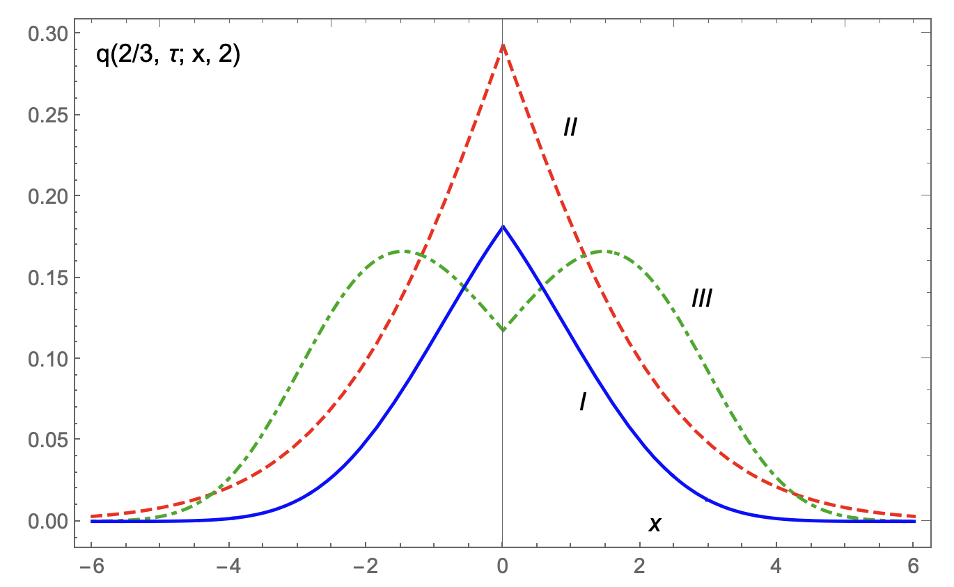
Figure 1: The density $q(2/3,\tau;x,2)$ for various $\tau$. The red dashed curve (no. II) represents $\lim_{\tau\to 0}q(2/3,\tau;x,t)=N(2/3;x,2)$ given by Eq. (32) where we set $B=1$. The green dot-dashed curve (no. III) exhibits $\lim_{\tau\to\infty}q(2/3,\tau;x,2)=W(2/3;x,2)$ which is given by Eq. (33) with $a=1$. The blue solid curve (no. I) illustrates the solution of generalized Cattaneo equation (22). The function $f_{0}$ is given by the representation Eq. (31).

In Fig. 1 we present also the special cases of $q(\alpha,\tau;x,t)$ obtained by taking its limits of $\tau\to 0$ and $\tau\to\infty$. For $\tau\ll 0$ we can use Eq. (6) in which $N(x,\xi)=(2\sqrt{B})^{-1}f_{0}(1/2;|x|/\sqrt{B},\xi)$. Then, we employ (KAPenson16, , Eqs. (29)-(32)). That allows one to find

$$N(\alpha;x,t)=(2\sqrt{B})^{-1}f_{0}(\alpha/2;|x|/\sqrt{B},t),$$ (32)

equal to (EBarkai01, , Eq. (16)). Eq. (32) can be also obtained by using the technique presented in KGorska12 ; EBarkai01 . For $\tau\gg 1$, with $a=(B/{\tau})^{1/2}$,  Eq. (27) reads

$$W(\alpha;x,t)=(2a)^{-1}f_{0}(\alpha;|x|/a,t).$$ (33)

For $a=1$ it is equivalent, e.g., to (YuLuchko13, , Eq. (9)) or (YuLuchko19, , Eq. (33)), which employ the Mainardi function $M_{\alpha}(u)=u^{-1-1/\alpha}g_{\alpha}(u^{-1/\alpha})/\alpha$. Eqs. (32) and (33), although at the first glance look quite similar, in fact differ significantly. The difference, clearly seen in Fig. 1, has its origin in the value of the first parameter which is either $\alpha/2$ in Eq. (32) or $\alpha$ in Eq. (33). For the solutions to the (standard) anomalous diffusion equation given by Eq. (32) we always observe one maximum localized at $x=0$ while for the diffusion-wave equation we get either one or two maxima. The number of maxima in question depends on the value which the parameter $\alpha$ takes on: for $\alpha\in(0,1/2]$ we deal with one maximum localized at $x=0$ while for $\alpha\in(1/2,1]$ we have two maxima localized at $x=\pm x_{m}$ (the curve no. III in Fig 1; $x_{m}=1.463$). Here we remind that such behaviour was noticed and discussed e.g. in YFujita90 ; YuLuchko13 in the context of propagation velocity characterizing diffusion phenomena.

(c) The solution $q_{1}(\tau;x,t)$ of the example (a) is defined on the compact support. This situation becomes opposite, as seen from (b), when the memory effects, in fact meaning the time non-locality, come to play. To investigate this change we will consider the example (b) perturbed by the non-negative constant parameter $\epsilon$, i.e., a linear combination of memories which define examples (a) and (b). Such new memory has the form $\hat{\gamma}(z)=z^{\alpha-1}+\epsilon$ where $\alpha\in(0,1]$ and $\epsilon\geq 0$. That leads to

$$f_{0}(\alpha,\epsilon; \,\xi,t)=\mathcal{L}^{-1}[(z^{\alpha-1}+\epsilon)\operatorname{e}^{-\xi z^{\alpha}}\operatorname{e}^{-\xi\epsilon z};t]$$

$$=\Theta(t-\epsilon\xi)\left(\frac{t}{\alpha\xi}-\epsilon\frac{1-\alpha}{\alpha}\right)g_{\alpha}(\xi,t-\epsilon\xi),$$ (34)

where the inverse Laplace transforms have been calculated applying twice the Laplace convolutions once for $z^{\alpha-1}\exp(-\xi z^{\alpha})$ and another time for $\exp(-\xi z^{\alpha})$. The occurrence of $\Theta(t-\epsilon\xi)$ guarantees that the second argument of $g_{\alpha}(\xi,t-\epsilon\xi)$ is non-negative. Consequently, it changes the infinite range integral given by Eq. (22) into the integral over the finite range. Thus, we get

$$q_{z^{\alpha-1}+\epsilon}(\tau;x,t)\equiv q(\alpha,\tau,\epsilon;x,t)=\int_{0}^{t/\epsilon}\!\!q_{\rm C}(\tau;x,\xi)\\ \times\left(\frac{t}{\alpha\epsilon\xi}-\frac{1-\alpha}{\alpha}\right)g_{\alpha}(\xi,t-\epsilon\xi)\!\operatorname{d\!}\xi.$$ (35)

Because this integral is defined in the finite region and $q_{\rm C}(\tau;x,\xi)$ contains the $\delta$-Dirac distributions as well as the Heaviside step function we get the relation between $x$ and $t$ in which $|x|\leq at$ for $\epsilon=1$. Hence, we can suspect that $q(\alpha,\tau,\epsilon;x,t)$ for $\epsilon>0$ is nonzero only in the finite subset of $x$. The size of this subset enlarges as the evolution goes on and its dimension depends on the time $t$ passed, as well as on the constants $a$ and $\epsilon$. The above relation between $x$ and $t$ disappears for $\epsilon\to 0$ and $q(\alpha,\tau,0;x,t)$ becomes nonzero for all $x\in\mathbb{R}$, i.e., we arrive at the example (b). Analytic calculations of Eq. (35) are difficult to be done so we present only numerical results obtained using Mathematica 12. Results are plotted on Fig. 2 obtained for rational $\alpha=l/k$ and Eqs. (23) and (29) employed.

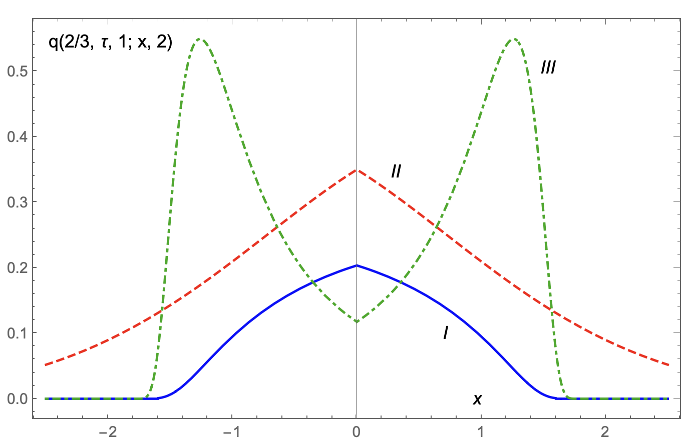
Figure 2: The figure represents the PDF $q(2/3,\tau,1;x,2)$ (the blue solid curve, no. I) and its limits with respect to $\tau$. For small $\tau$ it goes to $N(2/3,1;x,2)$ (the red dashed curve, no. II) and for large $\tau$ it tends to $W(2/3,1;x,2)$ (the green dot-dashed curve, no. III). The function $f_{0}$ is calculated using Eq. (IV) in which the one-sided Lévy stable distribution $g_{l/k}(\sigma)$, $0<l<k$, is given by Eq. (29).

In Fig. 2, besdes of the example of $q(\alpha,\tau,\epsilon;x,t)$ for $\epsilon>0$ (the blue curve, no. I), there are also presented its two special cases in which we consider the limits of $q(\alpha,\tau,\epsilon;x,t)$ for $\tau\to 0$ and $\tau\to\infty$. In the first case the PDF $q(\alpha,0,\epsilon;x,t)$ is equal to Eq. (35) where instead of $q_{\rm C}(\tau;x,\xi)$ sits $N(x,\xi)$. This limit is denoted as $N(\alpha,\epsilon;x,t)$ and it is presented in Fig. 2 by the red curve no. II. In the next limit we have $q(\alpha,\infty,\epsilon;x,t)$ denoted as $W(\alpha,\epsilon;x,t)$. It is given though Eq. (27) in which $f_{0}$ is equal to Eq. (IV) . The PDF $W(\alpha,\epsilon;x,t)$ is illustrated by the green curve with no. III.

V Discussion

The main results of the paper may be resumed two-fold. Firstly, we shed new light on the subordination approach and present its modification naturally appearing in the description of anomalous diffusion. Secondly, we provide an explicit example of the memory functions ${\hat{\gamma}}(s)$ which if put into generalized, time smeared, Cattaneo equation lead to solutions sharing the basic property obeyed by solutions of the standard Cattaneo equation, namely it do vanish outside the compact region $\Delta(x,t)$, i.e. $q_{\hat{\gamma}}(\tau;x,t)=0$ if $x,t\notin\Delta(x,t)$.

The integral decompositions of solutions to the diffusion-like equations are rooted in procedures which allow to transform solutions found in the Fourier/Laplace domain to the physical $(x,t)$ space. If merged with principles of the subordination approach the integral decompositions serve as a tool which makes it possible to prove the probabilistic character of such obtained solutions. However, as has been warned in recent papers, this claim has to be treated carefully. The reason is that integral decompositions constructed according to the standard procedures are not always sufficient to confirm the probabilistic interpretation of $q_{\hat{\gamma}}(\tau;x,t)$ in a complete and correct way AChechkin21 ; IMSokolov05 ; TSandev18 . The commonly proposed integral decompositions are assumed to reflect the fact that the Brownian motion, described by the normal distribution $N(x,\xi)$ parametrized in physical space $x$ and operational time $\xi$, is subordinated by a random process which links the physical and operational times through the relation given by an infinite divisible distribution $f_{\tau}(\xi,t)$. Despite the fact that the normal distribution $N(x,\xi)$ satisfies all conditions needed to be a suitable PDF there exist examples for which the second component of such a way obtained decomposition, namely the function $f_{\tau}(\xi,t)$, is not the PDF TSandev18 . In our paper we propose another type of integral decomposition within which, instead of the normal distribution $N(x,t)$, there appears the fundamental solution of the standard Cattaneo equation $q_{\rm C}(\tau;x,t)$. The latter satisfies all requirements to be a suitable PDF and using it allows us to keep the subordinator $f_{0}(\xi,t)$ which usually accompanies $N(x,t)$. Correctness and validity of such introduced modification of the subordination approach is confirmed by showing that in the limits of small and large $\tau$ the PDF $q_{\hat{\gamma}}(\tau;x,t)$ reconstructs solutions $N_{\hat{\gamma}}(x,t)$ and $W_{\hat{\gamma}}(x,t)$ of the time smeared diffusion and wave equations.

The second important result flows out from the analysis of three examples presented in the paper and illustrating the role played by memory functions. Our examples allow us to suspect which shape the memory functions should have in order to judge if the solution of generalized Cattaneo equation $p_{\hat{\gamma}}(\tau;x,t)$ has non-zero values only in the compact region and vanishes outside of it. Thus, we propose the answer on the open problem about vanishing of the solution of the anomalous diffusion and/or diffusion-wave equations. As the first example we consider the standard Catteneo equation in which the second and first time derivatives are strictly localized. Solution to this equation $q_{1}(\tau;x,t)\equiv q_{\rm C}(\tau;x,t)$ is nonzero for any $x\in\Delta(x,t)$. The situation changes radically if we introduce the memory functions $\eta(t)$ and $\gamma(t)$. For the predominantly used model of memory functions, i.e. $\eta\propto t^{1-2\alpha}$ and $\gamma(t)\propto t^{-\alpha}$, $\alpha\in(0,1]$, the PDF $q_{z^{\alpha-1}}(\tau;x,t)=q(\alpha,\tau;x,t)$ is always nonzero for $x\in\mathbb{R}$. Analogical situation takes place for both limit cases, $\tau\to 0$ and $\tau\to\infty$ - the solutions $N(\alpha;x,t)$ as well as $W(\alpha;x,t)$ are nonzero for all $x\in\mathbb{R}$. Different behaviour we face if consider the second example perturbed by a strictly localized term - this we model by introducing memories $\eta(t)=\epsilon\delta(t)+t^{1-2\alpha}/\Gamma(2-2\alpha)$ and $\gamma(t)=\epsilon\delta(t)+t^{-\alpha}/\Gamma(1-\alpha)$, $\epsilon\geq 0$, anytime with $\alpha\in(0,1]$. Obviously, putting $\epsilon=0$ we come back to the second example and to the generalized Cattaneo equation which solution is nonzero for $x\in\mathbb{R}$. For $\epsilon>0$ the solution behaves differently: $q_{z^{\alpha-1}+\epsilon}(\tau;x,t)\equiv q(\alpha,\tau,\epsilon;x,t)$ does not vanish only for $x\in\Delta(x,t/\epsilon)$. Such compact region appears in the limit of $\tau\to\infty$ for which $q(\alpha,\infty,\epsilon;x,t)=W(\alpha,\epsilon;x,t)$ but does not happen for $\tau\to 0$ in which $q(\alpha,0,\epsilon;x,t)$ equals $N(\alpha,\epsilon;x,t)$.

Sec. III.1 extends results of the seminal paper HDWeymann67 . It shows that for $|x|\ll at$ it is not possible to differentiate between the plots of solutions to standard anomalous diffusion RMetzler19 ; YuLuchko19 and generalized Cattaneo equations KGorska20 ; EAwad20 ; JMasoliver17 ; JMasoliver16 ; ACompte97 . Having this at hand one cannot show which of patterns fits the experimental data better. Thus, if we are limited to just mentioned range of $x$, we are unable to decide which random walk model, either continuous time random walk (CTRW) or, alternatively, continuous time persistent random walk (CTPRW) is more appropriate to describe phenomena under consideration. These models differ by the probability densities. In CTRW the random walker arrives to the localization $(x,t)$ moving along one channel whereas in CTPRW it may arrive to $(x,t)$ through two channels. This dichotomy results in the differences of waiting time and jump PDFs. In CTRW the waiting time PDF in the Laplace domain reads $\hat{\psi}(s)=[1+\tau s^{2}\hat{\gamma}^{2}(s)+s\hat{\gamma}(s)]$ whereas in CTPRW we have $\hat{\psi}_{\pm}=[1+2\tau s\hat{\gamma}(s)]^{-1}$ KGorska20 . The CTRW and CTPRW models differ also by the jump PDFs, in CTRW it depends only on the position $x$ whereas for CTPRW it depends both on the position $x$ and time $t$.

VI Conclusions

In our opinion observations made in Sec. IV and Disscusion justify to formulate the conjecture:

This is the appearance of the $\delta$-Dirac distribution in memory function $\eta(t)$ (so involving the constituent leading to strictly localized second time derivative) which ensures that the generalized Cattaneo equation can be interpreted in terms of the wave equation. In such a case its solutions share properties characteristic for the wave-like propagation and are nonzero only in a compact region defined by motion of the wave fronts.

The above expresses the claim that the second time derivative present in the evolution equation prevents any particle to spread out beyond the compact region similarly like it takes place for the Cattaneo equation SGoldstein51 . We are going to verify this conjecture by checking for which forms of memory function (if any besides of one discussed in Sec. IIIA) the wave behavior of $p_{\hat{\gamma}}(\tau;x,t)$ may be observed. We expect that further analysis of wave phenomena seen in solutions to the Cattaneo equation, like the Doppler studied recently in Ref. YuPovstenko21 , will appear helpful to understand better wave properties of solutions to the generalized Cattaneo equation.

Figs. 1 and 2 illustrate the cusp-containing and bimodal behavior (occurring in dependence to the value of $\tau$) of solutions relevant for examples (b) and (c) of Sec. IV. Such patterns have been noted in semi-relativistic time evolution equations investigated in classical and quantum mechanics, to mention the Salpeter equation CBeck03 ; KKowalski11 ; KAPenson18 ; MVChubynsky14 ; RJain17 . In studies of anomalous diffusion cusp-containing and bimodal behavior of PDF-interpreted solutions have appeared useful and quite popular in considerations dealing with the so-called Brownian but non-Gaussian models SHapca09 ; BWang09a ; BWang12 ; AVChechkin17 ; WWang20 ; WWang20a ; RMetzler20 . Our approach suggests possible modifications of results presented in MVChubynsky14 ; AVChechkin17 ; VSposini18 ; EBPostnikov20 devoted to the concept of diffusing diffusivity model being recently a hot topic in anomalous diffusion research stimulated by tracking of single particle diffusion. In diffusing diffusivity models the diffusion coefficient $B$ of the tracer particle is supposed to evolve in time and its time behaviour is (usually) assumed to take the shape which the coordinate of a Brownian particle in a gravitational field has. In such a case the distribution function $P(x,t)$ of a system of traced particles is given by

$$P(x,t)=\int_{0}^{\infty}N(x,t|B)p_{B}(B)\operatorname{d\!}B,$$ (36)

where $N(x,t|B)\equiv N(x,t)$ is used to denote explicitly the dependence on $B$. The PDF $p_{B}(B)$ is usually assumed to be $\exp(-B/\langle B\rangle)/\langle B\rangle$ with $\langle B\rangle$ being the effective diffusivity. Hence, $P(x,t)$ is given by the Laplace distribution, see SHapca09 ; BWang09a ; AVChechkin17 . Currently investigated modifications of Eq. (36), discussed in AVChechkin17 ; VSposini18 ; AGCherstvy21 , rely on changing $p_{B}(B)$ but keeping $N(x,t|B)$. Based on results presented in our paper we would like to propose another modification of Eq. (36), namely to substitute $p_{\hat{\gamma}}(\tau;x,t)$ instead of $N(x,t|B)$ but still preserve the exponential form of $p_{B}(B)$. This will lead to the cusp-containing and bimodal behaviour which appropriately chosen memory function may cause that diffusion will be restricted to the compact region.

Appendix A The completely monotonic and completely Bernstein functions

The function $\widehat{h}(s)$, $s\in\mathbb{R}_{+}$, is a completely Bernstein function (CBF) if:

• $\widehat{h}(s)$ and its derivative $[\widehat{h}(s)]^{\prime}$ are non-negative functions and, moreover, all derivatives of $[\widehat{h}(s)]^{\prime}$ alternate RLSchilling10 , namely

  $$(-1)^{n-1}\widehat{h}^{(n)}(s)\geq 0,\quad n=1,2,\ldots;$$

• $\widehat{h}(s)$ and $s/\widehat{h}(s)$ have the representation given by the Stieltjes transform RLSchilling10 .

Alternative criterion says that $\widehat{h}(s)$ is CBF if $s/\widehat{h}(s)$ is CBF RLSchilling10 .

The completely monotonic function (CMF) $\widehat{H}(s)$ are non-negative function of a non-negative argument whose all derivatives exist and alternate, i.e.

$$(-1)^{n}\widehat{H}^{(n)}(s)\geq 0,\quad n=0,1,\ldots.$$

The Bernstein theorem uniquely and mutually connects CMF with the non-negative function defined on $\mathbb{R}_{+}$ by the Laplace transform:

$$\widehat{H}(s)=\int_{0}^{\infty}\operatorname{e}^{-st}H(t)\operatorname{d\!}t,$$

where $\widehat{H}(s)$ is CMF DVWidder46 ; HPollard44 ; ANKochubei11 .

Appendix B The relation between the infinitely divisible distribution and the Bernstein-class functions: BF as well as CBF

The relation between the CBF and infinitely divisible function is expressed by (RLSchilling10, , Lemma 9.2). It say that the measure $g$ on $[0,\infty)$ is infinitely divisible iff $\mathcal{L}[g;\lambda]=\exp[-f(\lambda)]$ where $f$ is CBF.

Appendix C The Efross theorem

We quote here the Efross theorem AEfross35 ; LWlodarski52 ; UGraf04 ; KGorska12a ; AApelblat21 which is the generalization of the convolution theorem for the Laplace transform. According to it if $G(z)$ and $g(z)$ are analytic functions, ${\cal L}[h_{1}(x,\xi);z]=\hat{h}_{1}(x,z)$ and

$${\cal L}[h_{2}(\xi,t);z]=\int_{0}^{\infty}h_{2}(\xi,t)\operatorname{e}^{-zt}\operatorname{d\!}t=\widehat{G}(z)\operatorname{e}^{-\xi\hat{k}(z)},$$

then

$$\widehat{G}(z)\hat{h}_{1}(x,\hat{k}(z))=\int_{0}^{\infty}\!\Big{[}\!\int_{0}^{\infty}\!\!h_{1}(x,\xi)h_{2}(\xi,t)\operatorname{d\!}\xi\Big{]}\operatorname{e}^{-zt}\operatorname{d\!}t.$$

Thus, we can conclude that

$${\cal L}^{-1}[\widehat{G}(z)\hat{h}_{1}(x,\hat{k}(z));t]=\int_{0}^{\infty}\!\!h_{1}(x,\xi)h_{2}(\xi,t)\operatorname{d\!}\xi.$$ (37)

We illustrate this theorem by deriving Eq. (22). As $\hat{h}_{1}(x,z)$ we take $F(x,z)$ from Eq. (18). That gives $h_{1}(x,\xi)={\cal L}^{-1}[F(x,z);\xi]$. This inverse Laplace transform can be calculated by using the formulas placed in (JMasoliver19, , Appendix A) and/or (YuPovstenko21, , Appendix B). Namely,

$${\cal L}^{-1}[(z^{2}-\lambda^{2})^{-1/2}\exp[-\mbox{$\frac{|x|}{a}$}(z^{2}-\lambda^{2})^{1/2}];\xi\}\\ =\Theta(\xi-\mbox{$\frac{|x|}{a}$})I_{0}[\mbox{$\frac{1}{2\tau}$}(\xi^{2}-\mbox{$\frac{x^{2}}{a^{2}}$})^{1/2}]$$ (38)

and

$${\cal L}^{-1}[z(z^{2}-\lambda^{2})^{-1/2}\exp[-\mbox{$\frac{|x|}{a}$}(z^{2}-\lambda^{2})^{1/2}];\xi\}\\ =\delta(\xi-\mbox{$\frac{|x|}{a}$})+\Theta(\xi-\mbox{$\frac{|x|}{a}$})\frac{\lambda\xi}{(\xi^{2}-\mbox{$\frac{x^{2}}{a^{2}}$})^{1/2}}\\ \times I_{1}[\mbox{$\frac{1}{2\tau}$}(\xi^{2}-\mbox{$\frac{x^{2}}{a^{2}}$})^{1/2}],$$ (39)

where $\lambda=(2\tau)^{-1}$. Due to the property of $\delta$-Dirac distribution we have that $\delta(\xi-|x|/a)=a\delta(a\xi-|x|)$ gives two peaks at $x-a\xi$ and $x+a\xi$. Thus, it can be expressed as $a[\delta(x-a\xi)+\delta(x+a\xi)]$ and

$$h_{1}(x,\xi)=\operatorname{e}^{\xi/(2\tau)}q_{\rm C}(x,\xi).$$ (40)

According to Subsec. II.2 we have that $\widehat{G}(z)=\hat{\gamma}(z)$ and $\hat{k}(z)=g(z)$ given by Eq. (19). That leads to

$$\begin{split}h_{2}(\xi,t)&={\cal L}^{-1}[\hat{\gamma}(z)\operatorname{e}^{-\xi z\hat{\gamma}(z)-\xi/(2\tau)};t]\\ &=\operatorname{e}^{-\xi/(2\tau)}f_{0}(\xi,t),\end{split}$$ (41)

where we used the property of inverse Laplace transform saying that

$${\cal L}^{-1}[\hat{H}(z+\lambda);t]=\operatorname{e}^{-t\lambda}{\cal L}^{-1}[\hat{H}(z);t].$$ (42)

Inserting Eqs. (40) and (41) into Eq. (37) we derive $q_{\hat{\gamma}}(\tau;x,t)$.

Appendix D The passage between Eqs. (14) and (22)

Eq. (14) in which we insert Eq. (15) where $\hat{M}_{\hat{\gamma}}(z)$ leads to Eq. (12). If we separate $z\hat{\gamma}(z)$ from $\hat{M}_{\hat{\gamma}}(z)$ then we can express $f_{\tau}(\xi,t)$ as

$$f_{\tau}(\xi,t)=\mathcal{L}^{-1}\{\hat{\gamma}(z)[1+\tau z\hat{\gamma}(z)]\operatorname{e}^{-\xi z\hat{\gamma}(z)[1+\tau z\hat{\gamma}(z)]};t\}.$$

Using the Efross theorem in which $\hat{k}(z)=z\hat{\gamma}(z)$, $\hat{G}(z)=\hat{\gamma}(z)$, and $\hat{h}_{1}(\xi,y)=(1+\tau y)\exp[-\xi y(1+\tau y)]$, we represent $f_{\tau}(\xi,t)$ in the form

$$f_{\tau}(\xi,t)=\int_{0}^{\infty}\!\!\mathcal{L}^{-1}[(1+\tau y)\operatorname{e}^{-\xi y(1+\tau y)};u]\operatorname{d\!}u\\ \times\mathcal{L}^{-1}[\hat{\gamma}(z)\operatorname{e}^{-uz\hat{\gamma}(z)};t].$$ (43)

Then, we rewrite Eq. (14) as

$$q_{\hat{\gamma}}( \tau;x,t)=\int_{0}^{\infty}\!\!\mathcal{L}^{-1}[(1+\tau y)$$

$$\times\int_{0}^{\infty}\!\!N(x,\xi)\operatorname{e}^{-\xi y(1+\tau y)}\operatorname{d\!}\xi;u]\,f_{0}(u,t)\operatorname{d\!}u,$$ (44)

where the integral over $\xi$ goes inside the first inverse Laplace transform in Eq. (43). Due to (APPrudnikov-v1, , Eq. (2.3.16.2)) we get $\int_{0}^{\infty}\!\!\operatorname{e}^{-a/\xi-b\xi}\xi^{-1/2}\operatorname{d\!}\xi=\sqrt{\pi/b}\operatorname{e}^{-2\sqrt{ab}}$. This formula allows one to rewrite Eq. (D) as

$$q_{\hat{\gamma}}(\tau;x,t)=\int_{0}^{\infty}\!\!\mathcal{L}^{-1}\{F[x,y+1/(2\tau)];u\}f_{0}(u,t)\operatorname{d\!}u,$$ (45)

where $F(x,g)$ is given by Eq. (18). Thereafter, we can repeat calculation in Eq. (II.2) in which instead of $z\hat{\gamma}(z)$ we have $y$ and we use property Eq. (42). At the consequence of it we obtain the integral decomposition given by Eq. (22).

Appendix E Derivation of Eq. (25)

We start with the series definition of modified Bessel function of the first kind. That allows us to write

$$I_{\nu}(\mbox{$\frac{1}{2a\tau}$}\sqrt{a^{2}t^{2}-x^{2}})\\ =\sum_{n\geq 0}\frac{[t/(4\tau)]^{2n+\nu}}{n!\Gamma(\nu+n+1)}\Big{(}1-\frac{x^{2}}{a^{2}t^{2}}\Big{)}^{n+\frac{\nu}{2}}.$$ (46)

Applying now the binomial sum to $\{1-[x/(at)]^{2}\}^{n}$ we can express the modified Bessel function in Eq. (46) as

$$\Big{(}1-\frac{x^{2}}{a^{2}t^{2}}\Big{)}^{\nu/2}\sum_{n\geq 0}\sum_{r=0}^{n}\frac{[t/(4\tau)]^{2n+\nu}}{\Gamma(\nu+n+1)}\frac{(-\mbox{$\frac{x^{2}}{a^{2}t^{2}}$})^{n-r}}{r!(n-r)!}.$$ (47)

Then, we observe that the double sum $\sum_{n\geq 0}\sum_{r=0}^{n}$ can be rewritten in the form $\sum_{r\geq 0}\sum_{n=r}^{\infty}$. Setting $n-r=j$ we have

$$\Big{(}1-\frac{x^{2}}{a^{2}t^{2}}\Big{)}^{\!\nu/2}\sum_{j\geq 0}\frac{1}{j!}\Big{(}\!-\frac{x^{2}}{4\tau a^{2}t}\Big{)}^{\!j}\\ \times\sum_{r\geq 0}\frac{[t/(4\tau)]^{2r+\nu+j}}{\Gamma(\nu+j+r+1)r!}$$ (48)

The series definition of the modified Bessel function $I_{\nu}(\cdot)$ allow us to write

$$I_{\nu}(\mbox{$\frac{1}{2a\tau}$}\sqrt{a^{2}t^{2}-x^{2}})\\ =\Big{(}1-\frac{x^{2}}{a^{2}t^{2}}\Big{)}^{\!\nu/2}\sum_{j\geq 0}\frac{1}{j!}\Big{(}\!-\frac{x^{2}}{4\tau a^{2}t}\Big{)}^{\!j}I_{\nu+j}\Big{(}\frac{t}{2\tau}\Big{)},$$

which agree with (APPrudnikov-v2, , Eq. (5.8.3.1)). Using the asymptotic form of modified Bessel function for large $t/(2\tau)$, which boils down to $I_{\nu}[t/(2\tau)]=[\tau/(\pi t)]^{1/2}\exp[t/(2\tau)]$, we obtain Eq. (25).

References

- (1) N. Sperelakis, Cell Physiology Sourcebook: Essentials of Membrane Biophysics, 4th ed. (Academic Press, 2012).
- (2) J.-H. Jeon, V. Tejedor, S. Burov, E. Barkai, C. Selhuber-Unkel, K. Berg-Sørensen, L. Oddershede, and R. Metzler, In Vivo Anomalous Diffusion and Weak Ergodicity Breaking of Lipid Granules, Phys. Rev. Lett. 106, 048103 (2011).
- (3) J. F. Reverey, J.-H. Jeon, H. Bao, M. Leippe, R. Metzler, and C. Selhuber-Unkel, Superdiffusion dominates intracellular particle motion in the supercrowded cytoplasm of pathogenic Acanthamoeba castellanii, Sci. Rep. 5, 11690 (2015).
- (4) C. Fuchs, Inference of Diffusion Processes with Applications in Life Sciences (Springer Verlag, Berlin/Heidelberg, 2013).
- (5) J. Cejka, A. Corma, and S. Jones, Zeolites and Catalysis: Synthesis, Reactions and Applications, (Wiley-VCH, 2010).
- (6) A. K. Blackadar, Turbulence and Diffusion in the Atmosphere: Lectures in Environmental Sciences, (Springer Verlag, Berlin/Heidelberg, 1997).
- (7) A. M. Gusak, Diffusion Controlled Solid State Reactions in Alloys, Thin Films and Nano Systems, (Wiley-VCH Verlag GmbhCo, KGaA, Wien, 2010).
- (8) D. Gupta, Diffusion Processes in Advanced Technological Materials, (William Andrews Publishing, Norwich, New York Springer Verlag Berlin Heidelberg, 2005).
- (9) J. Janssen, O. Manca, R. Manca, Applied Diffusion Processes from Engineering to Finance (Wiley-ISTE, 2013).
- (10) J. W. Haus and K. W. Kehr, Diffusion in regular and disordered lattice, Phys. Rep. 150, 263 (1987).
- (11) R. Metzler, J.-H. Jeon, A. G. Cherstvy, and E. Barkai, Anomalous diffusion models and their properties: non-stationarity, non-ergodicity, and ageing at the centenary of single particle tracking, Phys. Chem. Chem. Phys. 16, 24128, 2014.
- (12) R. Metzler, Brownian motion and beyond: first-passage, power spectrum, non-Gaussianity, and anomalous diffusion, J. Stat. Mech. 114003, 2019; https://doi.org/10.1088/1742-5468/ab4988.
- (13) K. Górska, A. Horzela, E. K. Lenzi, G. Pagnini, and T. Sandev, Generalized Cattaneo (telegrapher’s) equations in modeling the anomalous diffusion phenomena, Phys. Rev. E 102, 022128 (2020).
- (14) C. R. Cattaneo, Sulla conduzione del calore, Atti. Sem. Mat. Fis. Univ. Modena, 3, 83 (1948).
- (15) C. R. Cattaneo, Sur une forme de l’equation de la chaleur eliminant le paradoxe d’une propagation instantanee’, Comptes Rendus de l’Académie des Sciences 247, 431 (1958).
- (16) J. A. Stratton, Electromagnetic Theory (McGraw-Hill Book Co., New York, 1941).
- (17) P. M. Morse and H. Feshbach, Methods of Theoretical Physics, Ch. 7.4, (Mac Grow-Hill Book Company, New York/Toronto/London, 1953).
- (18) J. Masoliver and G. H. Weiss, Finite-velocity diffusion, Eur. J. Phys. 17, 190 (1996).
- (19) T. Sandev, Z. Tomovski, J. L. Dubbeldam, and A. V.Chechkin, Generalized diffusion-wave equation with memory kernel, J. Phys. A: Math. Theor. 52, 015201 (2019).
- (20) Yu. Luchko, F. Mainardi, and Yu. Povstenko, Propagation speed of the maximum of the fundamental solution to the fractional diffusion-wave equation, Comput. Math. Appl. 66, 774 (2013).
- (21) Yu. Luchko and F. Mainardi, Fractional diffusion-wave phenomena, in Handbook of Fractional Calculus with Applications, vol. 5, part B, pp. 71-98 (De Gruyer, Berlin/Boston, 2019).
- (22) H. C. Fogedby, Langevin equations for continuous time Lévy flights, Phys. Rev. E 50, 1657 (1994).
- (23) I. M. Sokolov, Solution of a class of non-Markovian Fokker-Planck equation, Phys. Rev. E 66, 041101 (2002).
- (24) I. M. Sokolov and J. Klafter, From diffusion to anomalous diffusion: A century after Einstein’s Brownian motion, Chaos 15, 026103 (2005).
- (25) A. Baule and R. Friedrich, Joint probability distribution for a class of non-Markovian processes, Phys. Rev. 71, 026101 (2003).
- (26) A. V. Chechkin and I. M. Sokolov, On relation between generalized diffusion and subordination schemes, Phys. Rev. E 103, 032133 (2021).
- (27) R. L. Schilling, R. Song, and Z. Vondracek, Bernstein Functions (De Gruyter, Berlin, 2010).
- (28) Y. Z. Povstenko, Fractional Thermoelasticity (Springer, New York, 2015).
- (29) A. Compte and R. Metzler, The generalized Cattaneo equation for the description of anomalous processes, J. Phys. A: Math. Gen. 30, 7277 (1997).
- (30) E. Awad and R. Metzler, Crossover dynamics from superdiffusion to subdiffusion: model and solutions, Fract. Calc. Apply. Anal. 23, 55 (2020).
- (31) A. Giusti, Dispersion relations for the time-fractional Cattaneo-Maxwell heat equation, J. Math. Phys. 59, 013506 (2018).
- (32) T. Kosztolowicz, Cattaneo-type sub diffusion-reaction equation, Phys. Rev. E 90, 042151 (2014).
- (33) K. D. Lewandowska and T. Kosztolowicz, Application of generalized Cattaneo equation to model sub diffusion impedance, Acta Phys. Pol. B 39, 1211 (2008).
- (34) A. Stanislavsky and K. Weron, Stochastic tools hidden behind the empirical dielectric relaxation laws, Rep. Prog. Phys. 80, 036001 (2017).
- (35) A. Stanislavsky and A. Weron, Control of the transistent subdiffusion exponent at short and long times, Phys. Rev. Research 1, 023006 (2019).
- (36) S. Bochner, Harmonic Analysis and the Theory of Probability (Univ. of California Press, Berkeley/Los Angeles, 1955).
- (37) A. M. Efross, The application of the operational calculus to the analysis, Mat. Sb. 42, 699 (1935), in Russian.
- (38) Ł. Włodarski, Sur une formule de Efros, Studia Math. 13, 183 (1952).
- (39) U. Graf, Applied Laplace Transforms and z-Transforms for Sciences and Engineers (Birkhäuser, Basel, 2004).
- (40) K. Górska and K. A. Penson, Lévy stable distributions via associated integral transform, J. Math. Phys. 53, 053302 (2012).
- (41) A. Apelblat and F. Mainardi, Application of the Efros theorem to the function represented by the inverse Laplace transform of , Symmetry 13, 354 (2021).
- (42) J. B. Keller, Diffusion at finite speed and random walks, PNAS 101(5), 1120 (2004).
- (43) M. Kac, A stochastic model related to the telegrapher’s equation, Rocky Mountains J. Math. 4(3), 497 (1974).
- (44) G. H. Weiss, Some applications of persistent random walks and the telegrapher’s equation, Physica A 311, 381 (2002).
- (45) J. Masoliver, Fractional telegrapher’s equation from fractional persistent random walks, Phys. Rev. E 93, 052107 (2016).
- (46) J. Masoliver and K. Lindenberg, Continuous time persistent random walk: a review and some generalizations, Eur. Phys. J. B 90, 107 (2017).
- (47) H. D. Weymann, Finite Speed of Propagation in Heat Condition, Diffusion, and Viscous Shear Motion, Am. J. Phys. 35, 488 (1967).
- (48) M. A. Olivares-Robles and L. S. Garcia-Colin, On Different Derivations of Telegrapher’s Type Kinetic Equations, J. Non-Equilib. Thermodyn. 21, 361 (1996).
- (49) M. V. Chubynsky and G. W. Slater, Diffusing Diffusivity: A Model for Anomalous, yet Brownian, Diffusion, Phys. Rev. Lett. 113, 098302 (2014).
- (50) A. V. Chechkin, F. Seno, R. Metzler, and I. M. Sokolov, Brownian yet Non-Gaussian Diffusion: From Superstatistics to Subordination of Diffusing Diffusivities, Phys. Rev. X 7, 021002 (2017).
- (51) V. Sposini, A. V. Chechkin, F. Seno, G. Pagnini, and R. Metzler, Random diffusivity from stochastic equations: comparison of two models for Brownian yet non-Gaussian diffusion , New J. Phys. 20, 043044 ( 2018).
- (52) E. B. Postnikov, A. V. Chechkin, and I. M. Sokolov, Brownian yet non-Gaussian diffusion in heterogeneous media: from superstatistics to homogenization, New J. Phys. 22, 063046 (2020).
- (53) R. Jain and K. L. Sebastian, Diffusing diffusivity: a new derivation and comparison with simulations, J. Chem. Sci. 129, 929 (2017).
- (54) A. G. Cherstvy, H. Safdari, and R. Metzler, Anomalous diffusion, nonergodicity, and ageing for exponentially and logarithmically time-dependent diffusivity: striking differences for massive versus massless particles, J. Phys. D: Appl. Phys. 54, 195401 (2021).
- (55) K. A. Penson and K. Górska, On the properties of Laplace transform originating from one-sided Lévy stable laws, J. Phys. A: Math. Theor. 49, 065201 (2016).
- (56) K. A. Penson and K. Górska, Exact and explicit probability densities for one-sided Lévy stable distributions, Phys. Rev. Lett. 105, 210604 (2010).
- (57) K. Górska and A. Horzela, The Volterra type equations related to the non-Debye relaxation, Commun. Nonlinear Sci. Numer. Simulat. 85, 105246 (2020).
- (58) E. Barkai, Fractional Fokker-Planck equation, solution, and application, Phys. Rev. E 63, 046118 (2001).
- (59) K. Górska, K. A. Penson, D. Babusci, G. Dattoli, and G. H. E. Duchamp, Operator solutions for fractional Fokker-Planck equations, Phys. Rev. E. 85, 031138 (2012).
- (60) Y. Fujita, Integrodifferential equation which interpolates the heat equation and the wave equation, Osaka J. Math. 27, 309 (1990).
- (61) S. Goldstein, On diffusion by discontinuous movements, and on the telegraph equation, Quart. J. Mech. Appl. Math. 4(2), 129 (1951).
- (62) C. Beck and E. G. D. Cohen, Superstatistics, Physica A 322, 267 (2003).
- (63) K. Kowalski and J. Rembielinski, Salpeter equation and probability current in the relativistic Hamiltonian quantum mechanics, Phys. Rev. A 84, 012108 (2011).
- (64) K. A. Penson, K. Górska, A. Horzela, and G. Dattoli, Quasi-Relativistic Heat Equation via Lévy Stable Distributions: Exact Solutions, Ann. Phys. (Berlin) 530, 1700374 (2018).
- (65) W. Wang, A. G. Cherstvy, X. Liu, and R. Metzler, Anomalous diffusion and nonergodicity for heterogeneous diffusion processes with fractional Gaussian noise, Phys. Rev. E 102, 012146 (2020).
- (66) W. Wang, A. G. Cherstvy, A. V. Chechkin, S. Thapa, F. Seno, X. Liu, and R. Metzler, Fractional Brownian motion with random diffusivity: emerging residual nonergodicity below the correlation time, J. Phys. A: Math. Theor. 53, 474001 (2020).
- (67) R. Metzler, Superstatistics and non-Gaussian diffusion, Eur. Phys. J. Special Topics 229, 711 (2010).
- (68) D. V. Widder, The Laplace Transform (Princeton University Press, London, 1946).
- (69) H. Pollard, The Bernstein-Widder theorem on completely monotonic functions, Duke Math. J. 11, 427 (1944).
- (70) A. N. Kochubei, General fractional calculus, evolution equations, and renewal processes, Integr. Eq. Oper. Theory 71, 583 (2011).
- (71) J. Masoliver, Telegraphic processes with stochastic resetting, Phys. Rev. E 99, 012121 (2019).
- (72) Yu. Povstenko and M. Ostoja-Staszewski, Doppler effect described by the solutions of the Cattaneo thelegraphers equation, Acta Mech. 232, 725 (2021).
- (73) A. P. Prudnikov, Yu. A. Brychkov, O. I. Marichev, Integrals and Series. Special Functions, vol. 2. (Gordon and Breach, Amsterdam, 1998).
- (74) A. P. Prudnikov, Yu. A. Brychkov, O. I. Marichev, Integrals and Series. Elementary Functions, vol. 1. (Gordon and Breach, Amsterdam, 1998).
- (75) S. Hapca, J. W. Crawford, and I. M. Young, Anomalous diffusion of heterogeneous populations characterized by normal diffusion at the individual level, J. R. Soc. Interface 6, 111 (2009).
- (76) B. Wang, S. M. Anthony, S. C. Bae, and S. Granick, Anomalous yet Brownian, Proc. Natl. Acat. Sci. U. S. A. 106, 15160 (2009).
- (77) B. Wang, J. Kuo, S. C. Bae, and S. Granick, When Brownian diffusion is not Gaussian, Nat. Matter 11, 481 (2012).