Hubble-induced phase transitions on the lattice with applications to Ricci reheating

Abstract

Using 3+1 classical lattice simulations, we follow the symmetry breaking pattern and subsequent non-linear evolution of a spectator field non-minimally coupled to gravity when the post-inflationary dynamics is given in terms of a stiff equation-of-state parameter. We find that the gradient energy density immediately after the transition represents a non-negligible fraction of the total energy budget, steadily growing to equal the kinetic counterpart. This behaviour is reflected on the evolution of the associated equation-of-state parameter, which approaches a universal value $1/3$, independently of the shape of non-linear interactions. Combined with kination, this observation allows for the generic onset of radiation domination for arbitrary self-interacting potentials, significantly extending previous results in the literature. The produced spectrum at that time is, however, non-thermal, precluding the naive extraction of thermodynamical quantities like temperature. Potential identifications of the spectator field with the Standard Model Higgs are also discussed.

1 Introduction

The appearance of tachyonic instabilities is an ubiquitous phenomenon in the physics of the very early Universe, being generically associated with the amplification of quantum fluctuations. Typical examples include natural and new inflation models [1, 2, 3, 4], preheating scenarios with trilinear interactions [5, 6], spontaneous symmetry breaking settings such as hybrid inflation [7, 8, 9, 10] and second-order phase transitions [11].

On general grounds, a tachyonic instability emerges whenever a mass eigenvalue in an interacting or self-interacting theory becomes negative. This transition can be caused by a bare mass parameter in the action or effectively induced by the expectation value of a given field or operator. In this context, models in which the instability is triggered by a non-minimal coupling to gravity have recently received considerable attention.

Hubble-induced phase transitions for spectator fields have been advocated to address several phenomenological aspects such as the generation of the observed matter-antimatter asymmetry [12], the formation of topological defects with observable gravitational wave backgrounds [13, 14], the onset of the hot big bang era [15, 16, 17] or the non-thermal production of dark matter [18, 19]. The main assumption behind these proposals is the existence of a cosmological expansion era with a stiff equation-of-state parameter ($w>1/3$) prior to the beginning of radiation domination.  This unusual equation of state induces a change of sign in the Ricci scalar and hence in the effective mass for the spectator field, triggering its displacement towards new time-dependent minima appearing at large field values.

In many instances, the evolution of the spectator field during Hubble-induced phase transitions is discussed in terms of an homogeneous component rolling down an effective potential and eventually oscillating around the new symmetry-breaking minima in a fully coherent fashion [15, 16, 17]. This naive picture is, however, inaccurate [7, 8]. On the one hand, it fails to capture one of the main features of spontaneous symmetry breaking: the production of topological defects [13]. On the other hand, the dynamics of the system is not dominated by an homogeneous component, but rather by the rapid amplification of long wavelength fluctuations that become relevant well before the field reaches the new minima of the potential [14]. Among other effects, this has important consequences for the virialization and thermalization of the system.

In order to verify and assess the relevance of the aforementioned features, we explore here, for the first time, the non-linear dynamics of Hubble-induced phase transitions using $3+1$ classical lattice simulations. To this end, we focus on a $Z_{2}$ symmetric spectator field non-minimally coupled to gravity, albeit our results can be easily extended to other global symmetry breaking patterns.

The present analysis differs in various aspects from previous studies in the context of hybrid inflation and phase transitions, for which lattice simulations are also available (see e.g. [7, 8, 9, 10, 11]), and multifield inflation with non-minimal couplings [21, 22]. First, the tachyonic mass leading to the spontaneous breaking of the aforementioned $Z_{2}$ symmetry is time-dependent. Second, the system is completely characterized by a single physical scale, the Hubble rate, which controls both the dilution and the tachyonic enhancement of perturbations. When numerical tools are brought to bear, we find also several interesting outcomes:

1. The Hubble-induced tachyonic instability leads to the formation of regions with positive and negative field values separated by domain wall configurations. These domains melt periodically at every field oscillation to reappear again just slightly distorted.

2. The time-dependent character of the symmetry-breaking minima prevents the usual stabilization around them, giving rise to a bi-modal distribution pattern that survives for a large number of oscillations.

3. Although the energy transfer to gradients is initially just a small fraction of the total energy density, it grows monotonically at the expense of the interaction and potential contributions. This leads to a final virialized state in which the kinetic energy density of the spectator field equals its gradient counterpart.

4. The virialization process is associated with a smooth turbulent regime, similar to that in Refs. [23, 24, 25, 26]. The continuous population of ultraviolet (UV) modes by this mechanism translates into an effective equation of state $w_{\chi}\simeq 1/3$. Combined with kination, this allows for the onset of radiation domination for general interacting potentials. This contrasts with the naive expectation following from the homogeneous approximation, where this transition is only possible for a quartic interaction [17].

5. Even if the late-time evolution of the spectator coincides with that of a radiation fluid, the associated spectrum of perturbations remains highly non-thermal for an extended period of time, precluding the naive extraction of thermodynamical quantities like temperature.

The paper is organized as follows. In Section 2, we introduce the basic ingredients of the model, leaving for Section 3 the description of the rapid amplification of the spectator field fluctuations through the Hubble-induced tachyonic instability. This classicalization process is essential for the analysis of the subsequent non-linear stage, which we study in Section 4 via $3+1$ classical lattice simulations. The implications of our findings for the onset of radiation domination are discussed in Section 5. Section 6 contains a summary of our main theoretical assumptions and future research lines, including a discussion on the possibility of identifying the spectator field with the Standard Model Higgs. Finally, our conclusions are presented in Section 7.

2 Non-minimally coupled spectator field

A cosmological expansion epoch with a stiff equation-of state parameter ($w>1/3$) appears naturally in non-oscillatory quintessential inflation models aiming to provide a unified description of inflation and dark energy using a single degree of freedom [27, 28, 29, 30, 31, 32, 33, 34, 35, 36, 37, 38, 39, 40, 41]. In this type of scenarios, the absence of a potential minimum triggers generically a kination or deflation period immediately after the end of inflation. During this era, the total energy budget of the Universe is dominated by the kinetic energy density of the inflaton field, such that the global effective equation of state approaches $w\simeq 1$. Within this context, let us consider the following $Z_{2}$ symmetric action for an energetically subdominant spectator field $\chi$,

$$S_{\chi}=\int d^{4}x\sqrt{-g}\left[-\frac{1}{2}g^{\mu\nu}\partial_{\mu}\chi\partial_{\mu}\chi-\frac{1}{2}\xi R\chi^{2}-\frac{1}{4}\lambda\chi^{4}\right]\,,$$ (2.1)

where we have intentionally omitted a potential mass contribution which, if sufficiently small, will not play any essential role in the following discussions [12, 13, 14]. Here $R$ stands for the Ricci scalar constructed out of the metric $g_{\mu\nu}$ and $\xi$ and $\lambda$ are two dimensionless coupling constants that we will assume to be positive-definite in what follows.

The dynamics of the field $\chi$ is characterized by the Klein–Gordon equation,

$$\Box\,\chi-\xi R\chi-\lambda\chi^{3}=0\,,$$ (2.2)

together with the energy density and pressure following from the $00$ and $ii$ components of the associated energy-momentum tensor,

$$T^{(\chi)}_{\mu\nu}=D_{\mu}\chi D_{\nu}\chi-g_{\mu\nu}\left[\frac{1}{2}D^{\rho}\chi D_{\rho}\chi+\frac{\lambda}{4}\,\chi^{4}\right]+\xi\Big{[}G_{\mu\nu}+\left(g_{\mu\nu}\Box-D_{\mu}\,D_{\nu}\right)\Big{]}\chi^{2},$$ (2.3)

with $D_{\mu}$ the covariant derivative, $G_{\mu\nu}$ the Einstein tensor and $\Box=D^{\lambda}D_{\lambda}$ the d’Alambertian operator. Note that the contraction of $T^{(\chi)}_{\mu\nu}$ with arbitrary timelike vectors $u^{\mu}$ and $u^{\nu}$ is not guaranteed to be positive definite at all times [43, 44, 45, 46], thus violating the weak energy condition $T^{(\chi)}_{\mu\nu}u^{\mu}u^{\nu}\geq 0$ within this particular sector.

For a fixed flat Friedmann–Lemaître–Robertson–Walker metric $g_{\mu\nu}={\rm diag}(-1,a^{2}(t)\,\delta_{ij})$ with scale factor $a(t)$, we have

$$R=3(1-3w)H^{2}\,,\hskip 19.91692ptG_{00}=3H^{2}\,,\hskip 19.91692ptG_{ij}=3\,w\,H^{2}g_{ij}\,,\hskip 19.91692pt\Box\chi=-\ddot{\chi}-3H\dot{\chi}+\frac{\nabla^{2}}{a^{2}}\,,$$ (2.4)

with $H=\dot{a}/a$ the Hubble rate, the dots denoting derivatives with respect to the coordinate time $t$, and $w$ the global equation–of–state parameter. Using these expressions, we can rewrite Eqs. (2.2) and (2.3) as

$$\ddot{\chi}+3H\dot{\chi}-a^{-2}\nabla^{2}\chi+3\xi(1-3w)H^{2}\chi+\lambda\,\chi^{3}=0\,,$$ (2.5)

$$\rho_{\chi}=T_{00}=\frac{1}{2}\dot{\chi}^{2}+\frac{1}{2a^{2}}|\nabla\chi|^{2}+\frac{\lambda}{4}\,\chi^{4}+3\xi\left[H^{2}+H\partial_{t}-\frac{1}{3}\frac{\nabla^{2}}{a^{2}}\right]\chi^{2}\,,$$ (2.6)

$$p_{\chi}=\frac{1}{3a^{2}}\sum_{i}T_{ii}=\frac{1}{2}\dot{\chi}^{2}-\frac{1}{6a^{2}}|\nabla\chi|^{2}-\frac{\lambda}{4}\,\chi^{4}+3\xi\left[wH^{2}-\frac{1}{3}\left(\partial^{2}_{t}+2H\partial_{t}\right)+\frac{2}{9}\frac{\nabla^{2}}{a^{2}}\right]\chi^{2}\,.$$ (2.7)

As long as the energy density in the scalar field is small and the corrections to the Planck mass are negligible, the background dynamics can be characterized independently of the spectator field. In particular, the equation-of-state parameter in the above expressions can be well-approximated by that of the quintessential inflation field. Having this in mind, we can distinguish two regimes:

1. Inflation ($w=-1$): During this epoch, the Hubble-induced mass term in Eq. (2.5) is positive definite, making the spectator field heavy for sufficiently large values of the non-minimal coupling ($\xi\gtrsim 1/12$). This confines the $\chi$ field to the origin of its effective potential and suppresses the generation of isocurvature perturbations [12, 13].

2. Kination ($w=1$): The onset of a kinetic dominated era soon after the end of inflation triggers the spontaneous symmetry breaking of the $Z_{2}$ symmetry and the subsequent evolution of $\chi$ towards large field values, $|\chi_{\rm min}|=\left(6\xi/\lambda\right)^{1/2}H$. 

To study the dynamics of the spectator field in between these cosmological epochs, we will assume the inflation-to-kination transition to be instantaneous as compared with the evolution of the scalar field and parametrize the temporal dependence of the scale factor and the Hubble rate as

$$a=a_{\rm kin}\left[1+3H_{\rm kin}\left(t-t_{\rm kin}\right)\right]^{1/3}\,,\hskip 56.9055ptH=\frac{H_{\rm kin}}{1+3H_{\rm kin}(t-t_{\rm kin})}\,,$$ (2.8)

with $a_{\rm kin}$ and $H_{\rm kin}$ the values of these quantities at the onset of kinetic domination, arbitrarily defined at $t=t_{\rm kin}$. Performing now the change of variables

$$Y\equiv\frac{a}{a_{\rm kin}}\frac{\chi}{\,\chi_{*}}\,,\hskip 42.67912pt\vec{y}\equiv\,a_{\rm kin}\chi_{*}\,\vec{x}\,,\hskip 42.67912ptz\equiv\,a_{\rm kin}\chi_{*}\,\tau\,,$$ (2.9)

with $\chi_{*}\equiv\sqrt{6\xi}H_{\rm kin}$ and conformal time $\tau\equiv\int dt/a$, the spectator field action (2.1) becomes

$$S_{\chi}=\int d^{3}{\vec{y}}\,dz\,\left[\frac{1}{2}(Y^{\prime})^{2}-\frac{1}{2}|\nabla Y|^{2}\,+\,\frac{1}{2}M^{2}(z)Y^{2}-\frac{\lambda}{4}\,Y^{4}\right]\,,$$ (2.10)

with the primes denoting derivatives with respect to the dimensionless conformal time $z$ and the spatial derivatives understood now as taken with respect to the new spatial coordinates $\vec{y}$. All the explicit temporal dependence in (2.10) is included in the effective mass term

$$M^{2}(z)\equiv(1-6\xi)(\mathcal{H}^{2}+\mathcal{H}^{\prime})=(4\nu^{2}-1)\mathcal{H}^{2}\,,$$ (2.11)

constructed out of the comoving Hubble rate

$$\mathcal{H}(z)\equiv\frac{a^{\prime}(z)}{a(z)}=\frac{1}{2(z+\nu)}\,,\hskip 42.67912pt\mathcal{H}^{\prime}(z)=-2\mathcal{H}^{2}(z)\,,$$ (2.12)

with

$$\nu\equiv\sqrt{\frac{3\xi}{2}}$$ (2.13)

an integration constant ensuring that $z(t_{\rm kin})=0$. In terms of the new variables, the time-dependent minima of the potential are located at

$$|Y_{\rm min}|=\left(\frac{4\nu^{2}-1}{\lambda}\right)^{1/2}\mathcal{H}(z)\,,$$ (2.14)

while Eqs. (2.5) and (2.6) become

$$Y^{\prime\prime}-\nabla^{2}\,Y-M^{2}(z)Y+\lambda\,Y^{3}=0\,,\hskip 42.67912pt\rho_{\chi}=\mathcal{X}\,\rho_{Y}\,,\hskip 42.67912ptp_{\chi}=\mathcal{X}\,p_{Y}\,,$$ (2.15)

with $\mathcal{X}\equiv\chi_{*}^{4}(a_{\rm kin}/a)^{4}$ an overall rescaling factor. Here

$$\rho_{Y}\equiv K+G+V+I_{1}\,,\hskip 42.67912ptp_{Y}\equiv K-\frac{1}{3}G-V+I_{2}\,,$$ (2.16)

stand respectively for the dimensionless energy density and pressure of the $Y$-field with

$$K=\frac{1}{2}\left(Y^{\prime}-\mathcal{H}Y\right)^{2}\,,\hskip 28.45274ptG=\frac{1}{2}|\nabla Y|^{2}\,,\hskip 28.45274ptV=\frac{\lambda}{4}Y^{4},\\$$ (2.17)

$$I_{1}=2\nu^{2}\left[\mathcal{H}(Y^{2})^{\prime}-\mathcal{H}^{2}Y^{2}-\frac{1}{3}\nabla^{2}Y^{2}\right]\,,\hskip 14.22636ptI_{2}=2\nu^{2}\left[\mathcal{H}(Y^{2})^{\prime}-\mathcal{H}^{2}Y^{2}-\frac{1}{3}(Y^{2})^{\prime\prime}+\frac{2}{9}\nabla^{2}Y^{2}\right]\,,$$ (2.18)

the kinetic ($K$), gradient ($G$), potential ($V$) and interaction contributions ($I_{1}$,$I_{2}$) following from the corresponding terms in Eqs. (2.6) and (2.7). As anticipated after Eq. (2.3), the spectator energy density is not positive definite for non-vanishing $\nu$. Note, however, that the total energy density including the inflaton field and other potential matter components is positive definite at all times, as required by the $G_{00}$ component in (2.4).

3 Linear evolution of the quantum system

Immediately after symmetry breaking, the action (2.10) can be well approximated by that of a free scalar field with time dependent mass $M(z)$, making the problem exactly solvable. In this section, we follow the canonical formalism of Ref. [10], which has been applied to the present scenario in Ref. [14], where we refer the reader for a more detailed discussion. Expanding the $Y$ field in Fourier modes with wavenumber

$$\kappa\equiv|\vec{\kappa}|\equiv\frac{|\vec{k}|}{a_{\rm kin}\chi_{*}}\,,$$ (3.1)

and introducing position and momentum operators satisfying the usual equal-time commutation relations $\left[Y_{\vec{\kappa}}(z),\Pi_{\vec{\kappa}^{\prime}}(z)\right]=i\delta^{3}(\vec{\kappa}+\vec{\kappa}^{\prime})$, the quantum Hamiltonian following from Eq. (2.10) in the Gaussian approximation becomes the sum of an infinite set of harmonic oscillators,

$$H=\frac{1}{2}\int d^{3}\kappa\,\left[\Pi_{\vec{\kappa}}(z)\,\Pi^{\dagger}_{\vec{\kappa}}(z)+\omega_{\kappa}^{2}(z)\,Y_{\vec{\kappa}}(z)\,Y^{\dagger}_{\vec{\kappa}}(z)\right]\,,$$ (3.2)

with time-dependent dispersion relation

$$\omega_{\kappa}^{2}(z)\equiv\kappa^{2}-M(z)^{2}\,.$$ (3.3)

As clearly illustrated by this expression, the tachyonic instability induced by kinetic domination affects not only the zero mode of the scalar field but also all subhorizon modes below the time-dependent mass $M^{2}(z)$, i.e., those within a sliding window $\kappa_{\rm min}(z)\lesssim\kappa\lesssim\kappa_{\rm max}(z)$, with

$$\kappa_{\rm min}(z)=\mathcal{H}(z)\quad\quad{\rm and}\quad\quad\kappa_{\rm max}=(4\nu^{2}-1)^{1/2}\kappa_{\rm min}\,.$$ (3.4)

The evolution of this Gaussian quantum system is determined by the Heisenberg equations,

$$\frac{d}{dz}\begin{pmatrix}\Pi_{\vec{\kappa}}(z)\vspace{2mm}\cr Y_{\vec{\kappa}}(z)\end{pmatrix}=\begin{pmatrix}0&-\omega^{2}_{\kappa}(z)\vspace{2mm}\cr 1&0\end{pmatrix}\begin{pmatrix}\Pi_{\vec{\kappa}}(z)\vspace{2mm}\cr Y_{\vec{\kappa}}(z)\end{pmatrix}\,,$$ (3.5)

being all physical information encoded in the two-mode correlation functions at equal or different times,

$$\langle v^{I}_{\vec{\kappa}}(z)\,v^{J}_{\vec{\kappa}^{\prime}}(z^{\prime})\rangle=\Sigma^{IJ}_{\kappa}(z,z^{\prime})\,\delta^{3}({\vec{\kappa}}+{\vec{\kappa}^{\prime}})\,,$$ (3.6)

with $v_{\vec{\kappa}}\equiv\left(\Pi_{\vec{\kappa}}(z),Y_{\vec{\kappa}}(z)\right)^{T}$ and the brackets indicating a quantum average over the initial state. Using Eq. (3.5), we can express the correlation matrix $\Sigma^{IJ}_{\kappa}(z,z^{\prime})$ in (3.6) in terms of its value at any reference time $z_{r}$, namely [47, 48, 49, 10]

$$\Sigma_{\kappa}(z,z^{\prime})={\mathbf{M}}_{\kappa}(z)\,\Sigma_{\kappa}(z_{r},z_{r})\,{\mathbf{M}}^{T}_{\kappa}(z^{\prime})\,,\hskip 14.22636pt{\mathbf{M}}_{\kappa}(z)=\begin{pmatrix}\sqrt{\frac{2}{\kappa}}\,\textrm{Re}\,g_{\kappa}(z)&\sqrt{2\kappa}\,\textrm{Im}\,g_{\kappa}(z)\vspace{2mm}\cr-\sqrt{\frac{2}{\kappa}}\,\textrm{Im}\,f_{\kappa}(z)&\sqrt{2\kappa}\,\textrm{Re}\,f_{\kappa}(z)\end{pmatrix}\,,$$ (3.7)

with $f_{\kappa}$ a solution of the Schrödinger-like differential equation

$$f_{\kappa}^{\prime\prime}+\omega^{2}_{\kappa}(z)\,f_{\kappa}=0\,,$$ (3.8)

with initial conditions $f_{\kappa}(z_{r})$ and $f^{\prime}_{\kappa}(z_{r})$ and $g_{\kappa}\equiv if^{\prime}_{\kappa}$. Restricting ourselves to the large $\nu$ limit (cf. Section 6) and assuming the system to be initially in a vacuum state with $f_{\kappa}(z_{r}=0)=1/\sqrt{2\kappa}$ and $f^{\prime}_{\kappa}(z_{r}=0)=-i\sqrt{\kappa/2}$, the solution of Eq. (3.8) takes the compact form [14]

$$f_{\kappa}(z)=\sqrt{z+\nu}\left[A_{\kappa}\,\mathcal{J}_{\nu}(\kappa(z+\nu))-B_{\kappa}\,\mathcal{Y}_{\nu}(\kappa(z+\nu))\right]\,,$$ (3.9)

with $\mathcal{J_{\nu}}$ and $\mathcal{Y_{\nu}}$ the Bessel’s functions of the first and second kind,

$$A_{\kappa}={\cal Y}_{\nu}(\kappa\nu)\,\delta\,,\hskip 42.67912ptB_{\kappa}=\,{\cal J}_{\nu}(\kappa\nu)\,\delta-\frac{f_{\kappa}(0)}{\sqrt{\nu}{\cal Y}_{\nu}(\kappa\nu)}\,,$$ (3.10)

and

$$\delta=\frac{\pi f_{\kappa}(0)}{4\sqrt{\nu}}\left[1-2\nu+2\nu\left(\kappa\frac{{\cal Y}_{\nu-1}(\kappa\nu)}{{\cal Y}_{\nu}(\kappa\nu)}-\frac{f^{\prime}_{\kappa}(0)}{f_{\kappa}(0)}\right)\right]\,.$$ (3.11)

Using these expressions, we can easily evaluate the equal-time correlation matrix

$$\Sigma_{\kappa}(z,z)=\begin{pmatrix}|g_{\kappa}(z)|^{2}&F_{\kappa}(z)-\frac{i}{2}\vspace{3mm}\cr F_{\kappa}(z)+\frac{i}{2}&|f_{k}(z)|^{2}\end{pmatrix}\,,$$ (3.12)

with

$$F_{\kappa}(z)\equiv\frac{1}{2}\,\langle\Pi_{\vec{\kappa}}(z)\,Y_{\vec{\kappa}}^{\dagger}(z)+Y_{\vec{\kappa}}(z)\,\Pi_{\vec{\kappa}}^{\dagger}(z)\rangle={\rm Im}\,(f_{\kappa}^{*}g_{\kappa})$$ (3.13)

a WKB phase directly related to the Heisenberg uncertainty principle [47, 49, 48, 10]

$$\Delta Y_{\kappa}^{2}\,\Delta\Pi_{\kappa}^{2}=|F_{\kappa}(z)|^{2}+\frac{1}{4}\geq{\frac{1}{4}}\,\Big{|}\langle[Y_{\kappa}(z),\ \Pi^{\dagger}_{\kappa}(z)]\rangle\Big{|}^{2}\,.$$ (3.14)

For $|F_{\kappa}(z)|\gg 1$, the commutator $\langle\{Y_{\kappa}(z),\ \Pi_{\kappa}^{\dagger}(z)\}\rangle$ in this expression exceeds significantly the anticommutator $\langle|[Y_{\kappa}(z),\Pi_{\kappa}^{\dagger}(z)]|\rangle$,

$$\langle\{Y_{\kappa}(z),\ \Pi_{\kappa}^{\dagger}(z)\}\rangle\gg\langle|[Y_{\kappa}(z),\Pi_{\kappa}^{\dagger}(z)]|\rangle=\hbar\,,$$ (3.15)

meaning that the properties of the system can be well-approximated by those of a classical random field (see Fig. 1).

The equal-time correlation matrix (3.12) allows the computation of several related quantities characterizing the Gaussian random field [14]. Among those to be considered in the subsequent analysis, we can highlight the two-point correlation function obtained by Fourier transforming the diagonal entry $|f_{\kappa}(z)|^{2}$,

$$\zeta(\vec{y},z)\equiv\left\langle Y(\vec{y},z)Y(0,z)\right\rangle=\int\frac{d^{3}\kappa}{(2\pi)^{3}}\,e^{i\vec{\kappa}\cdot\vec{y}}\,|f_{\kappa}(z)|^{2}\,.$$ (3.16)

For a highly-symmetric spherical configuration and large $\nu$ values, the momentum integral in this expression can be computed explicitly, getting [14]

$$\zeta(r,z)\simeq\zeta(0,z)\,G_{1}(\kappa_{*}r)\,,$$ (3.17)

with

$$\zeta(0,z)\equiv Y^{2}_{\rm rms}(z)=\left(\frac{2\nu-1}{8\pi\nu}\right)^{2}\left(1+\frac{z}{\nu}\right)^{2\nu+1}\kappa_{*}^{2}(z)$$ (3.18)

the square of the time-dependent dispersion determining the root mean-square perturbation (rms), $\kappa_{*}(z)\equiv 2\sqrt{\nu+1}\,\kappa_{\rm min}(z)$ a typical momentum scale and

$$G_{1}(\kappa_{*}r)\equiv\sqrt{\frac{\pi}{2}}\frac{1}{\kappa_{*}r}\exp\left(-\frac{1}{2}\kappa^{2}_{*}r^{2}\right)\text{erfi}\left(\frac{\kappa_{*}r}{\sqrt{2}}\right)\,,$$ (3.19)

a shape function, with erfi the imaginary error function [50].

4 Non-linear evolution of the classicalized system

As we have seen in the previous section, the quantum evolution of the spectator field drives the low momenta modes in Fourier space into a highly occupied state where quantum averages can be well approximated by classical ones [10, 14]. This allows us to study the subsequent non-linear evolution using just classical lattice simulations, instead of more involved $2$-particle irreducible techniques [51, 52, 53].

4.1 Lattice discretization

Our approach relies on standard numerical methods common to lattice implementations of classical field dynamics and makes use of the LATfield2 library for parallel field theory simulations [54]. This framework has been widely used for the analysis of topological defects and validated thoroughly [55, 56, 57, 58, 59]. We discretize the classical nonlinear equations of motion in both space and time, solving them in a finite-volume cubic lattice of size $L$ and $N^{3}$ points uniformly distributed, with periodic boundary conditions $Y_{Njk}=Y_{0jk}$, $Y_{iNk}=Y_{i0k}$ and $Y_{ijN}=Y_{ij0}$. The lattice parameters $L$ and $N$ are chosen in such a way that all the relevant scales are sufficiently covered during the simulation time. In particular, the infrared (IR) lattice cutoff $\kappa_{\rm lattice,IR}=2\pi/L$ is chosen to be much smaller than the minimum value of the characteristic momentum scale during the tachyonic regime, $\kappa_{\rm lattice,IR}\ll\kappa_{*}(z_{\rm nl})$, while the UV lattice cutoff $\kappa_{\rm lattice,UV}=\sqrt{3}/2N\,\kappa_{\rm lattice,IR}$ is taken to exceed the maximum momentum excited by the tachyonic instability, $\kappa_{\rm lattice,UV}\simeq{\rm few}\times\kappa_{\rm max}(0)$.

A set of classical initial realizations is then evolved using the discretized equations of motion, with the expansion of the Universe assumed to be kination dominated. This evolution is completely deterministic, being the random character restricted only to the initial conditions inherited from the quantum treatment in Section 3. The numerical integration is started at a fixed time $z_{i}$ sufficiently advanced to guarantee that a large fraction of the modes have become classical but well before the time $z_{\rm nl}$,

$$\left(1+\frac{z_{\rm nl}}{\nu}\right)^{\nu+1/2}\simeq\frac{8\pi\nu^{2}}{(2\nu-1)\sqrt{3\lambda(\nu+1)}}\left(1-\frac{1}{4\nu^{2}}\right)^{1/2}\,,$$ (4.1)

at which non linearities become relevant and backreaction starts to affect the analytical results [14].

Figure 1: The amplitude of the WKB phase $|F_{\kappa}|$ in the correlation matrix (3.12) as a function of the dimensionless momentum $\kappa$ evaluated at three different times. For the benchmark point $\nu=10$, $\lambda=10^{-4}$, the quantum to classical transition takes place before the linear approximation ceases to be valid at $z_{\rm nl}(\nu,\lambda)=11$. The shaded areas mark the regions $|F_{\kappa}|\leq 10$ (darker) and $|F_{\kappa}|\leq 100$ (lighter). The dashed vertical lines indicate the values $\kappa_{\rm min}(z)$ and $\kappa_{\rm max}(z)$ in (3.4), with the same color coding as $F_{\kappa}(z)$.

The amplitude of all modes that have not become classical by the initialization time $z_{i}$ (namely those with $|F_{\kappa}|\lesssim 10$, cf. Fig. 1) is set to zero in our simulations. The remaining Fourier components are initialized according to a Rayleigh distribution with uniform random phase $\theta_{k}\in[0,2\pi]$ and dispersion $\sigma_{k}^{2}=|f_{k}|^{2}$, i.e.

$$P(|Y_{k}|)\,d|Y_{k}|\,d\theta_{k}=\exp\Big{(}\!-{\frac{|Y_{k}|^{2}}{\sigma_{k}^{2}}}\Big{)}\,{\frac{d|Y_{k}|^{2}}{\sigma_{k}^{2}}}\,{\frac{d\theta_{k}}{2\pi}}\,,\hskip 28.45274ptY_{k}^{\prime}=\frac{F_{k}(z_{i})}{|f_{k}(z_{i})|^{2}}\ Y_{k}\,.$$ (4.2)

Since the short distance variations of the field fluctuations are not relevant for the thermodynamics description we will be interested in, we will make use of the ergodic postulate to identify ensemble averages of a given operator ${\cal O}(\vec{y},z)$ with volume averages over the lattice volume $V=L^{3}$,

$$\langle{\cal O}(z)\rangle=\frac{1}{V}\int_{\,V}d^{3}y\,\,{\cal O}(\vec{y},z)\,.$$ (4.3)

In some cases, we will perform also suitable coarse-grainings on time with resolution $z_{0}$ and/or averages over $J$ realizations of the stochastic initial conditions,

$$\langle{\cal O}(z)\rangle=\frac{1}{J}\sum_{j=1}^{J}\frac{1}{z_{0}}\int^{z}_{z-z_{0}}dz\,\,\frac{1}{V}\int_{\,V}d^{3}y\,\,{\cal O}^{(i)}(\vec{y},z)\,.$$ (4.4)

Finally, we will define occupation numbers as [60, 61]

$${n}_{\vec{\kappa}}(t)=\left(|\Pi_{\vec{\kappa}}|^{2}\,|Y_{\vec{\kappa}}|^{2}\right)^{\frac{1}{2}}\,.$$ (4.5)

For non-tachyonic frequencies this definition coincides with that following from the correspondence principle. Indeed, in the classical limit, the occupation number of a mode is given by ${n}_{\vec{\kappa}}(t)=A/(2\pi)=\frac{1}{2}|\Pi_{\vec{\kappa}}|_{\rm max}||Y_{\vec{\kappa}}|_{\rm max}$ with $A$ the area of the ellipse encircled by the trajectory in phase space. Taking into account that the modes are oscillating at late times and assuming them to be weakly coupled, we can write $|\Pi_{\vec{\kappa}}|_{\rm max}=(2\,|{\Pi}_{\vec{\kappa}}|^{2})^{1/2}$ and $|Y_{\vec{\kappa}}|_{\rm max}=(2|Y_{\vec{\kappa}}|^{2})^{1/2}$, recovering Eq. (4.5).

4.2 Results

Figure 2: Spectator field growth for the benchmark point $\nu=10$, $\lambda=10^{-4}$. We display 2-dimensional sections of a fraction $V/8$ of the 3-dimensional simulation volume $V$ at times $z=5,\,10,\,15,\,20,\,25,\,60$, with the $z$-axis indicating the corresponding field value at each point in this surface. The black segment in the second panel indicates the typical scale of the highest peaks.

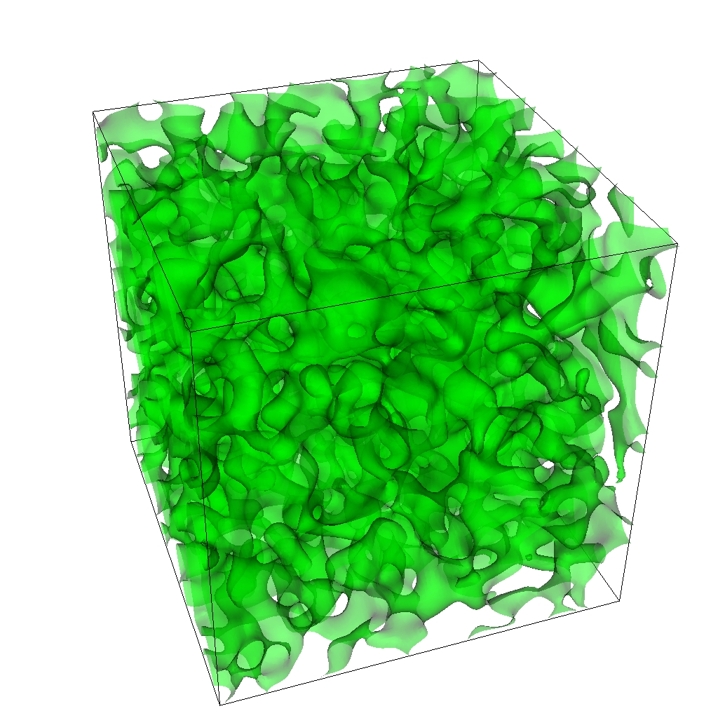
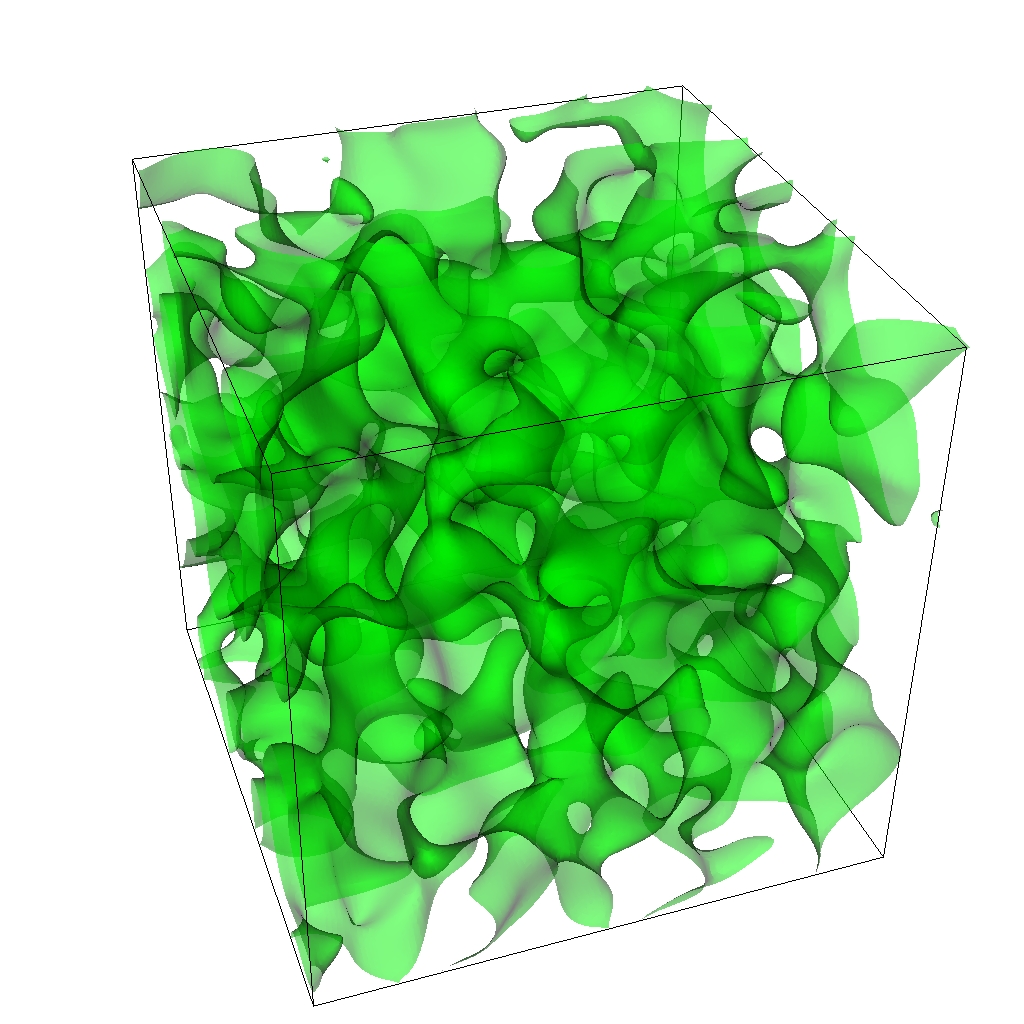
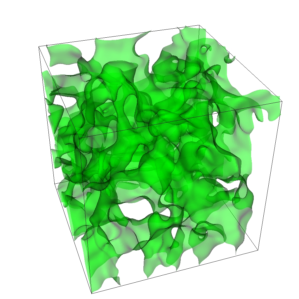
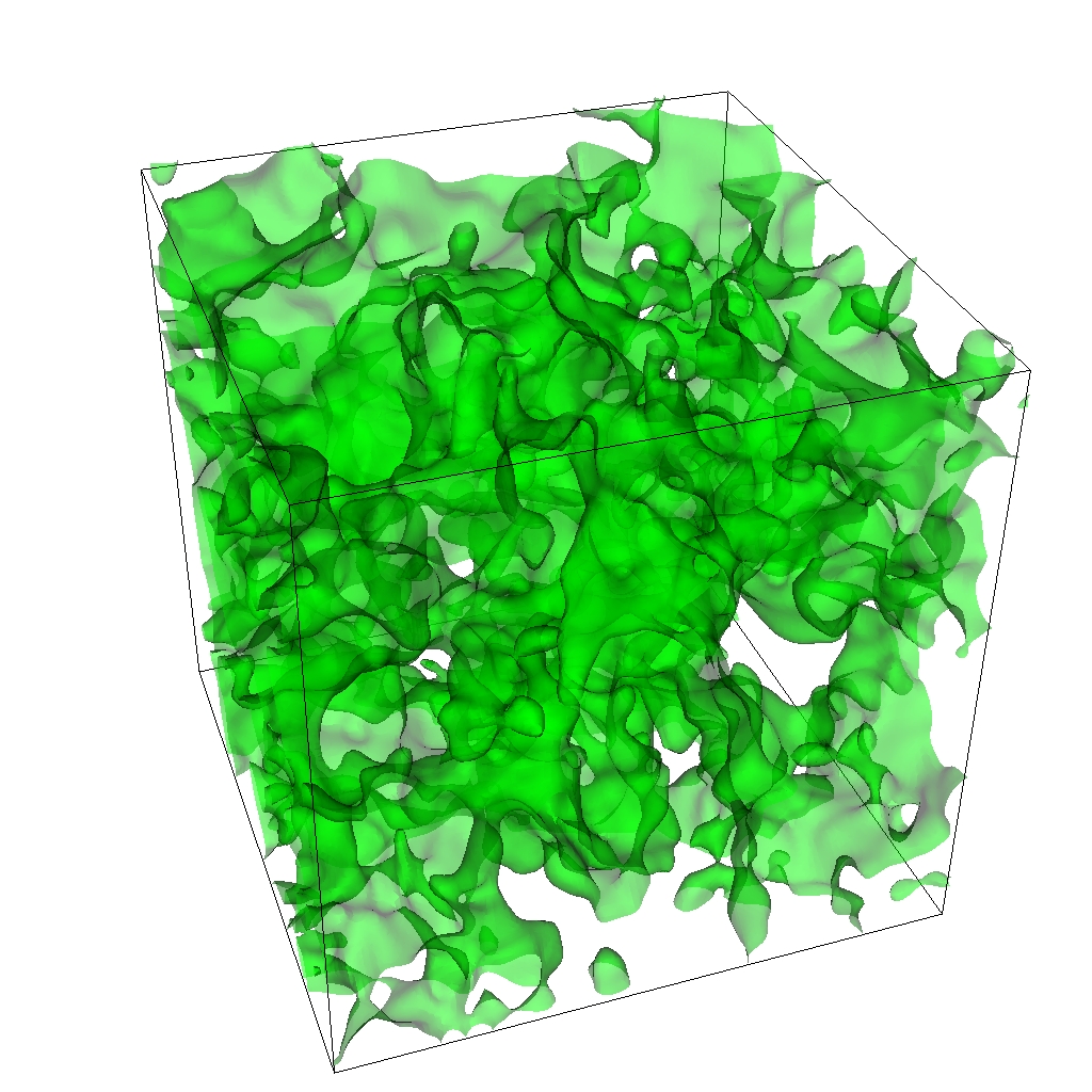
Figure 3: Domain wall configurations for the benchmark point $\nu=10$, $\lambda=10^{-4}$, obtained by plotting the 3-dimensional coordinates of the grid points with vanishing $Y$ at times $z=5,\,10,\,15,\,20,\,25,\,60$. As before, we display only $1/8$ of the total simulation volume.

To facilitate the comparison with the analytical results of Ref. [14], and without lack of generality, we concentrate in what follows on a benchmark point $\nu=10$, $\lambda=10^{-4}$, for which $z_{\rm nl}\simeq 11$.

Our simulations are carried out on a lattice with $N=1024$ and $L=0.185N$, which is initialized at $z=5$. With this choice of parameters the width of the domain walls is always larger than the lattice spacing, $dx=0.185$, making them resolvable throughout the entire simulation. The typical output is summarized in Fig. 2, where we present several 2-dimensional slices of the 3-dimensional lattice volume at different times. Although the initial conditions leading to these snapshots are random, the qualitative features displayed there are universal up to small spatial and temporal shifts. As anticipated above, an almost homogeneous Universe (1st panel) becomes rapidly separated into regions with positive and negative field values and typical size $L\lesssim\kappa_{*}^{-1}$, in agreement with the analytical result in Eq. (3.18) (2nd panel and 3rd panel). These macroscopic regions are melted at every field oscillation (4th panel) to reappear again slightly distorted (5th panel). As time proceeds, additional fluctuations are generated at smaller and smaller scales, giving eventually rise to a rather diffuse structure (6th panel). The domain walls separating regions of positive and negative $Y$ values can be explicitly detected. To this end, we plot in Fig. 3 the 3D coordinates of the grid points where $|Y|$ is close to zero. The displayed panels mirror the behaviour of Fig. 2. In particular, we observe a resilient formation and dissolution of domains.

A better characterization of the above symmetry-breaking picture can be achieved by considering the following observables:

1. Probability distribution: The total simulation volume containing the field value $Y$ at a given time $z$ is displayed in Fig. 4. This probability distribution is initially peaked at $Y=0$, with a dispersion relation given by $\sigma_{k}^{2}=|f_{k}|^{2}$. As time passes by, the distribution evolves towards the effective minima of the potential at large field values, eventually splitting in two. Contrary to other symmetry breaking scenarios [7, 8, 9, 10], the time-dependent character of the minima prevents the stabilization around them, giving rise to an oscillatory bi-modal pattern that survives for quite a number of oscillations.

   

   

   

   

   

   

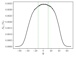
   Figure 4: Evolution of the probability distribution after symmetry breaking for the benchmark point $\nu=10$, $\lambda=10^{-4}$. We display snapshots at times $z=5,\,10,\,15,\,20,\,25,\,60$. The vertical green-dashed lines signal the location of the time-dependent minima, as given in Eq (2.14).

2. Time-dependent dispersion: The root mean-square perturbation $Y_{\rm rms}$ is displayed in Fig. 5 as a function of the dimensionless conformal time $z$ and the number of $e$-folds of kination, $N_{e}\equiv\ln(a/a_{\rm kin})$. Note that, as argued in Refs. [7, 8, 14], the picture of a homogeneously oscillating scalar field is incorrect when applied to spontaneous symmetry breaking. Indeed, when the initial value of the homogeneous component is close to zero, the classical rolling of the field is dominated by its quantum fluctuations, in agreement with the analytical result (3.18).

   

   Figure 5: Evolution of the volume-averaged lattice $Y_{\rm rms}$ for the benchmark point $\nu=10$, $\lambda=10^{-4}$ as compared to the analytical result (3.18), with $N_{e}$ the number of $e$-folds of kination.

3. Spectral distributions: The evolution of the occupation numbers (4.5) is shown in Fig. 6. We observe a rapid growth of infrared fluctuations at the early stages of symmetry breaking followed by a slower motion towards the UV due to the potential interactions. Note that the displayed behaviour is far from thermal. Indeed, thermal equilibrium can be only achieved once the occupation numbers in the infrared have significantly decreased to $n_{\kappa}\sim\lambda^{-1/4}$; a limit that notably exceeds our simulation time. On top of that, it is well known that classical lattice simulations cannot completely describe the approach to equilibrium due to the Rayleigh-Jeans divergence [62].

   A simple characterization of the UV cascade can be obtained by computing the average wavenumber [63]

   $$\kappa_{c}\equiv\frac{\int_{\kappa>\kappa_{0}}d^{3}\kappa\,|\kappa|\,|\Pi_{\vec{\kappa}}|^{2}}{\int_{\kappa>\kappa_{0}}d^{3}\kappa\,|\Pi_{\vec{\kappa}}|^{2}}\,,$$ (4.6)

   where we have intentionally excluded the infrared modes filled at the onset of the simulation, namely those below $\kappa_{0}=0.8$. As shown in Fig. 7, the momentum scale $\kappa_{c}$ is always smaller than the UV lattice cutoff, confirming that all relevant scales are well resolved throughout the entire simulation time.

   

   Figure 6: Time evolution of the occupation numbers (4.5) for the benchmark point $\nu=10$, $\lambda=10^{-4}$. Different colors correspond to different times, as indicated in the figure.

   

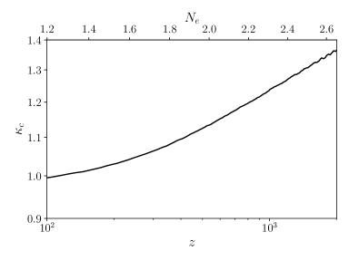
   Figure 7: Time evolution of the UV average momentum (4.6), with $N_{e}$ the number of $e$-folds of kination.

4. Energy budget: The evolution of the kinetic, gradient, potential and interaction contributions to the total spectator energy density is displayed in Fig. 8. After a rapid growth at early times and a violent oscillatory regime completely dominated by the interaction term, the system approaches an asymptotic state characterized by a large kinetic energy density. The smooth UV cascade in Fig. 6 translates then into a steady flow of energy from the interaction and potential terms to a slowly growing gradient component. As time passes by, the system relaxes towards a virialized state with $\braket{\textrm{K}}\simeq\braket{\textrm{G}}+2\braket{\textrm{V}}$, in agreement with the expectation for a quartic potential [64, 63].

   

   Figure 8: Evolution of the volume-averaged kinetic, gradient, potential and interaction contributions to the total spectator energy density for the benchmark point $\nu=10$, $\lambda=10^{-4}$, with $N_{e}$ the number of $e$-folds of kination. In order to facilitate the comparison, we display the absolute value of the interaction term $I_{1}$, since this is not positive definite at all times.

5. Equation-of-state parameter: The behaviour of the different energy density contributions is reflected also on the evolution of the associated equation-of-state parameter

   $$w_{\chi}\equiv\frac{\braket{p_{\chi}}}{\braket{\rho_{\chi}}}\,,$$ (4.7)

   which we display in Fig. 9. Since this quantity is rapidly oscillating as compared to the characteristic expansion rate, we perform here an additional coarse-graining in time, along the lines of Eq. (4.4). As shown in the left panel of the figure, the averaged equation of state is initially negative, becoming positive only during the tachyonic-to-oscillatory transition. This unusual behaviour is completely determined by the interactions terms in (2.18) (see also Fig. 8) and completely absent in standard minimally-coupled scenarios, where the equation of state is always positive definite. The small discrepancy between the lattice and the analytical estimate in Appendix A can be traced back to the fact that the latter assumes exact homogeneity and complete irrelevance of the non-linear potential terms while, albeit small initially, gradients are always present in the simulation and the potential terms can contribute. As shown in the right panel, $w_{\chi}$ approaches a value rather close to that of a radiation fluid ($w_{\chi}=1/3$) at late times. This behaviour is intrinsically related to the virialization process displayed in Fig. 8 and completely independent of whether the system is already thermalized or not [65].

   

   

   Figure 9: (Left) Evolution of the volume- and time-averaged equation-of-state parameter (4.7) immediately after symmetry breaking, with $N_{e}$ the number of $e$-folds of kination. (Right) Evolution of the same quantity at the latest stages of our simulation. The red horizontal line corresponds to the radiation value $1/3$.

6. Non-Gaussianities: To characterize the level of non-gaussianity in our scenario, we consider the so-called excess kurtosis, customarily defined as

   $$\Delta K\equiv\frac{\langle Y^{4}\rangle}{\langle Y^{2}\rangle^{2}}-3\,.$$ (4.8)

   

   Figure 10: Time-averaged evolution of the excess kurtosis (4.8) for the benchmark point $\nu=10$, $\lambda=10^{-4}$, with $N_{e}$ the number of $e$-folds of kination.

The above results should be understood as robust against variations of the initializing time $z_{i}$ and the lattice cutoffs. In particular, the temporal evolution of the different energy components is almost insensitive to the chosen initial condition and dominated by the modes lying far from the edges, where cutoff effects are subdominant.

5 Implications for the onset of radiation domination

The existence of a kination dominated era in quintessential inflation scenarios has strong implications for the onset of radiation domination [66, 38]. In particular, even if the energy density transferred to the spectator field,

$$\rho_{\chi}(z)=\mathcal{X}\,\rho_{Y}(z)=16\nu^{4}H_{\rm kin}^{4}\,\left(\frac{a_{\rm kin}}{a(z)}\right)^{4}\rho_{Y}(z)\,,$$ (5.1)

is initially very small, it will eventually become the dominant energy component due to the rapid decrease of the background energy density during this period,

$$\rho_{B}(z)=3M_{P}^{2}H^{2}(z)\equiv\mathcal{X}\rho^{(r)}_{B}(z)\,\,,\hskip 28.45274pt\rho^{(r)}_{B}(z)=\frac{3}{16\nu^{4}}\left(\frac{M_{P}}{H_{\rm kin}}\right)^{2}\left(\frac{a_{\rm kin}}{a(z)}\right)^{2}\,.$$ (5.2)

The comparison between these two quantities for the benchmark point $\nu=10$, $\lambda=10^{-4}$ is displayed in Fig. 11 for different values of the Hubble rate at the onset of kinetic domination. As shown there, even for tiny initial ratios $\rho_{\chi}(z_{i})/\rho_{B}(z_{i})\sim{\cal O}(10^{-9})$, the Universe enters radiation domination in less than $10$ $e$-folds of kination.

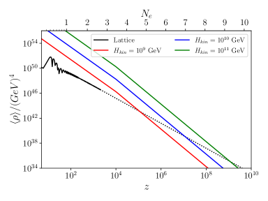
Figure 11: Comparison between the background energy density $\rho_{B}(z)$ in Eq. (5.2) for different $H_{\rm kin}$ scales and that transferred to the spectator field via the Hubble-induced symmetry breaking for the benchmark point $\nu=10$, $\lambda=10^{-4}$, with $N_{e}$ the number of $e$-folds of kination.

It is important to emphasize at this point that the onset of radiation domination is not related to the shape of the potential, as one could naively expect by considering the homogeneous approximation [17], but rather to the late-time hierarchy $\braket{V}\ll\braket{K},\braket{G}$ observed in Fig. 8. Indeed, for any virialized late-time scenario, [$1/2\langle{\dot{\chi}^{2}}\rangle=1/2\langle{(\nabla\chi/a)^{2}}\rangle+n\langle{V}\rangle$], involving a monomial potential $V\propto\chi^{2n}$ with $n\geq 1$ and negligible Hubble-induced interactions, one has [67, 68]

$$w_{\chi}=\frac{1}{3}+\frac{2}{3}\frac{(n-2)}{(n+1)+\langle(\nabla\chi/a)^{2}\rangle/\langle V\rangle}\,,$$ (5.3)

and therefore $w_{\chi}\to 1/3$ if $\langle(\nabla\chi/a)^{2}\rangle\gg\langle V\rangle$, in clear contrast with the value $w_{\chi}\to(n-1)/(n+1)$ obtained in the homogeneous limit $\langle(\nabla\chi/a)^{2}\rangle\ll\langle V\rangle$ [69, 70]. This can be explicitly verified by performing, for instance, a lattice simulation for a sextic potential $\frac{\sigma}{6\Lambda^{2}}\chi^{6}$, with $\sigma$ a coupling constant and $\Lambda$ a cutoff scale assumed to exceed $H_{\rm kin}$. In terms of the rescaled variables (2.9), the corresponding Klein-Gordon equation and potential energy density take the form

$$Y^{\prime\prime}-\nabla^{2}\,Y-M^{2}(z)Y+\sigma_{\rm eff}\,\,{\cal H}(z)\,Y^{5}=0\,,\hskip 28.45274ptV\equiv\frac{1}{6}\,\sigma_{\rm eff}\,\,{\cal H}(z)\,Y^{6}\,,$$ (5.4)

with

$$\sigma_{\rm eff}\equiv\sigma(2\nu)^{3}\left(\frac{H_{\rm kin}}{\Lambda}\right)^{2}$$ (5.5)

an effective dimensionless coupling constant.

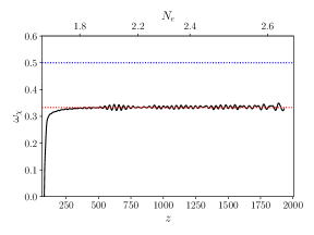
Figure 12: Energy distribution (left) and volume- and time-averaged equation of state (4.7) (right) for the sextic scenario in (5.4). The asymptotic behaviour of $w_{\chi}$ differs clearly from the homogeneous expectation $w_{\chi}=1/2$, approaching a radiation-like value $w_{\chi}=1/3$. This illustrates the importance of accounting for the production of IR perturbations and their subsequent UV cascade when studying Ricci reheating scenarios.

The evolution of the corresponding equation-of-state parameter $w_{\chi}$ for fiducial values $\nu=10$, $\sigma=0.01$ and $\Lambda=100\,H_{\rm kin}$ ($\sigma_{\rm eff}=0.008$) is displayed in Fig. 12. As expected, this quantity approaches a radiation-like value $w_{\chi}=1/3$ rather than the $w_{\chi}=1/2$ one following from the homogeneous approximation. Combined with kination, this observation allows for the generic onset of radiation domination for general interacting potentials, significantly extending the results of Ref. [17].

6 Assumptions and future research lines

We have performed several approximations to reduce the physical scenario to a baseline model that could be treated in a simple way with analytical and numerical techniques. Relaxing any of these assumptions opens new avenues for model building.

1. Symmetry group: We have assumed the spectator field to display a $Z_{2}$ symmetry, understanding this choice as a mere proof of concept of a much more general setting. In particular, we expect our results regarding the impact of perturbations on symmetry breaking and virialization to be extensible to more involved symmetry groups, provided that these are global.  The extension to local symmetries could, on the other hand, lead to new phenomenology, certainly worthy to explore.

2. Expansion of the Universe: We have assumed the inflation-to-kination transition to be instantaneous as compared to the temporal evolution of the spectator field. In practice, this corresponds to a quench approximation

   $$R(t<t_{\rm kin})>0\,,\hskip 28.45274ptR(t_{\rm kin}<t<t_{r})<0\,,$$ (6.1)

   with $t_{r}$ the symmetry restoration time. On top of that, we assumed the spectator energy density to be subdominant during kination, such that the Ricci scalar can be well approximated by an homogeneous function of time depending only on the inflaton equation of state. While this is certainly a reasonable assumption for the main stages described in this paper, it should be eventually taken into account for a precise determination of the onset of radiation domination.

3. Large $\nu$ approximation: In order to minimize the impact of horizon effects, we have focused on a large $\nu$ limit leading to a reasonable separation between ${\cal H}(z)$ and the typical momentum of the spectator field fluctuations, $\kappa_{*}(z)\equiv 2\sqrt{\nu+1}\,{\cal H}(z)$. This makes the integrated contribution of superhorizon modes reentering the horizon less and less important as compared with that of subhorizon scales never amplified by the inflationary dynamics, justifying the choice of a vacuum initial state with zero occupation numbers. We emphasize, however, that the asymptotic virialization observed in our simulations possesses an universal character, as we have explicitly verified by considering alternative initial conditions.

4. Parameter space: We have restricted ourselves to model parameters leading to a maximum $10\%$ correction to the reduced Planck mass, i.e. $\xi\chi_{\rm max}^{2}/M_{P}^{2}\leq 0.1$ [14]. Combined with the above two assumptions, this allows us to plausibly ignore metric fluctuations. Even within this self-consistency regime, our investigations are still limited to a small portion of the parameter space. Therefore, we cannot a priori exclude the existence of specific combinations of $\nu$ and $\lambda$ leading to different dynamics. We emphasize, however, that, given the decaying nature of the non-minimal coupling to gravity, the asymptotic behavior described in this paper is expected to be robust against variations of the model parameters. What could be affected at most is the duration of the tachyonic phase and the amount of defects that can be generated in the intermediate stages.

5. Couplings: We have assumed the spectator field to be decoupled or weakly coupled to an unspecified inflationary sector. Unless forbidden by any symmetry, this requires some level of fine-tuning. On top of that, we have ignored potential couplings to other matter components that must necessarily exist to recover the Standard Model content and other relevant species as dark matter [75], implicitly neglecting potential depletion and combined preheating effects [76, 77, 74, 78] that could modify the approach to equilibrium.

   An interesting possibility along this line of thought is the potential identification of the spectator field with the Standard Model Higgs, as first suggested in Ref. [15] within the context of kinetic domination. This association would lead to a rather minimalistic heating scenario not involving additional degrees of freedom beyond the Standard Model content. One of the recurrent arguments for restricting the parameter space of this appealing possibility [15, 17] is the apparent incompatibility of particle physics data with the absolute stability of the Standard Model vacuum below the Planck scale [79, 80]. We note, however, that the analyses of Ref. [15, 17] disregard implicitly the ambiguous relation between the Montecarlo reconstructed top quark mass and the actual top pole mass/Yukawa coupling entering in the renormalization group equations. As argued in Ref. [81], once this source of uncertainty is taken into account, it is perfectly possible for the Standard Model vacuum to be absolutely stable all the way up till the Planck scale. Indeed, the recent LHC measurements of the top pole mass point intriguingly towards this scenario [82, 83].

   Given the absolute stability of the Standard Model vacuum, the depletion of the spectator Higgs field in our setting is expected to proceed along the lines of Refs. [84, 85, 86, 87, 88], with potential differences associated to the bimodal pattern in Fig. 4, not accounted for in these papers. The thermalization of the resulting Standard Model species is estimated to be almost instantaneous [89, 15, 90, 91]

7 Conclusions

In this work, we have made a step forward towards the complete characterization of symmetry breaking in the context of Hubble-induced phase transitions, setting the stage for getting more reliable predictions to be eventually confronted with data. As a case of study, we investigated the full symmetry-breaking dynamics of a $Z_{2}$ spectator field non-minimally coupled to gravity. The transition from the unbroken to the broken phase is induced by a change of sign in the Ricci scalar as the Universe evolves from inflation to an era in which the equation-of-state parameter is stiff. In order to follow the non-linear evolution of the spectator field until the development of an equilibrium configuration, we made use of classical lattice simulations, being the corresponding initial conditions analytically obtained from a complete quantum field theory description of the early dynamics.

Our simulations allowed us to identify three different stages on the Hubble-induced symmetry breaking process. First, when the background acquires a stiff equation-of-state parameter immediately after the end of inflation, it induces a tachyonic instability for the spectator field fluctuations, which become amplified on infrared scales. This translates into the formation of rather homogeneous regions in real space separated by domain wall configurations. Second, as the field distribution splits and goes beyond the fading away minima of the effective potential, there appears a bi-modal oscillatory pattern that stays in place for a large number of oscillations. This stage is initially dominated by the non-minimal coupling to gravity, which become weaker and weaker as the Universe expands. Finally, we observe a long virialization stage, where the total energy density becomes democratically distributed among the kinetic and gradient components and the spectrum develops a turbulent cascade towards the UV. The equation-of-state of the spectator field approaches then a radiation-like value $w_{\chi}=1/3$, independently of the shape of the potential. The memory loss induced by this asymptotic stage does not imply that all the traces of the temporary Hubble-induced symmetry breaking are completely erased. Among other consequences, the temporal existence of topological defects may lead to the production of a detectable gravitational waves’ backgrounds [92, 93, 13] or baryogenesis [12], depending on the details of the symmetry breaking potential. We postpone the lattice characterization of these crucial aspects to a further publication.

Appendix A The homogeneous approximation

For the sake of completeness and in order facilitate the comparison with previous studies in the literature [15, 16, 17], we discuss here the evolution of the zero mode in the absence of quantum fluctuations. In this classical and homogeneous limit, the solution of the equation of motion (2.15) can be analytically obtained for both the tachyonic and pure quartic regimes. Assuming initial conditions $Y_{\rm kin}$ and $dY/dz|_{0}=Y_{\rm kin}/\nu$ and matching the solutions at the time

$$\frac{z_{\rm b}}{\nu}=\left(\frac{8}{\lambda Y_{\rm kin}^{2}}\frac{2\nu-1}{2\nu+1}\right)^{1/(2\nu+3)}-1\,,$$ (A.1)

at which the quadratic and quartic terms in the $Y$-field potential become equal, we get [14]

$$Y(z)\simeq\begin{cases}\frac{2\nu+1}{4\nu}Y_{\rm kin}\left(1+\frac{z}{\nu}\right)^{\nu+1/2}\hskip 68.2866pt{\rm for}\hskip 14.22636ptz\leq z_{b}\,,\\ Y_{\rm osc}\,\mathrm{cn}\left[\sqrt{\lambda}\,Y_{\rm osc}\,(z-z_{\rm osc}),\frac{1}{\sqrt{2}}\right]\hskip 34.1433pt{\rm for}\hskip 14.22636ptz>z_{b}\,,\end{cases}$$ (A.2)

where in the first expression we have neglected a subdominant decaying mode. Here $\mathrm{cn}$ stands for the Jacobi elliptic cosine,

$$Y_{\rm osc}=\frac{Y(z_{b})}{\sqrt{2}}\left[1+\left(1+\frac{2}{\beta^{2}}\frac{2\nu+1}{2\nu-1}\right)^{1/2}\right]^{1/2}$$ (A.3)

denotes the amplitude of the field at the time

$$z_{\rm osc}=z_{b}+\frac{1}{\,\beta\sqrt{\lambda}Y_{\rm osc}}\arccos\left(\frac{Y(z_{b})}{Y_{\rm osc}}\right)$$ (A.4)

at which the oscillatory part reaches its maximum ($z_{\rm osc}>z_{b}$) and $\beta=2\pi/T_{x}=0.8472$ is a numerical factor associated with the leading frequency of oscillation in the elliptic cosine series [14].

Although the solution (A.2) will break down as soon as gradients start to develop, it can be understood a relatively good description of the complete scenario at very early times, when all field fluctuations are still very close to the maximum of the effective potential. In particular, we can use it to estimate the value of the spectator field equation-of-state parameter (4.7) at the onset of kinetic domination. Taking into account Eqs. (2.16) and (2.17) at zero gradients, we get

$$w_{\chi,{\rm ini}}=1-\frac{4\nu}{3}\,,$$ (A.5)

which translates into a value $w_{\chi,{\rm ini}}=-12.3$ for $\nu=10$, in reasonable agreement with our lattice results and Ref. [17].

References

- [1] D. Cormier and R. Holman, Spinodal inflation, Phys. Rev. D 60 (1999) 041301, [hep-ph/9812476].
- [2] S. Tsujikawa and T. Torii, Spinodal effect in the natural inflation model, Phys. Rev. D 62 (2000) 043505, [hep-ph/9912499].
- [3] J. Rubio and E. S. Tomberg, Preheating in Palatini Higgs inflation, JCAP 04 (2019) 021, [1902.10148].
- [4] A. Karam, E. Tomberg and H. Veermäe, Tachyonic Preheating in Palatini Inflation, 2102.02712.
- [5] J. F. Dufaux, G. N. Felder, L. Kofman, M. Peloso and D. Podolsky, Preheating with trilinear interactions: Tachyonic resonance, JCAP 0607 (2006) 006, [hep-ph/0602144].
- [6] A. A. Abolhasani, H. Firouzjahi and M. M. Sheikh-Jabbari, Tachyonic Resonance Preheating in Expanding Universe, Phys. Rev. D 81 (2010) 043524, [0912.1021].
- [7] G. N. Felder, J. Garcia-Bellido, P. B. Greene, L. Kofman, A. D. Linde and I. Tkachev, Dynamics of symmetry breaking and tachyonic preheating, Phys. Rev. Lett. 87 (2001) 011601, [hep-ph/0012142].
- [8] G. N. Felder, L. Kofman and A. D. Linde, Tachyonic instability and dynamics of spontaneous symmetry breaking, Phys. Rev. D64 (2001) 123517, [hep-th/0106179].
- [9] E. J. Copeland, S. Pascoli and A. Rajantie, Dynamics of tachyonic preheating after hybrid inflation, Phys. Rev. D65 (2002) 103517, [hep-ph/0202031].
- [10] J. Garcia-Bellido, M. Garcia Perez and A. Gonzalez-Arroyo, Symmetry breaking and false vacuum decay after hybrid inflation, Phys. Rev. D67 (2003) 103501, [hep-ph/0208228].
- [11] J. T. Giblin, Jr., L. R. Price, X. Siemens and B. Vlcek, Gravitational Waves from Global Second Order Phase Transitions, JCAP 11 (2012) 006, [1111.4014].
- [12] D. Bettoni and J. Rubio, Quintessential Affleck-Dine baryogenesis with non-minimal couplings, Phys. Lett. B784 (2018) 122–129, [1805.02669].
- [13] D. Bettoni, G. Doménech and J. Rubio, Gravitational waves from global cosmic strings in quintessential inflation, JCAP 1902 (2019) 034, [1810.11117].
- [14] D. Bettoni and J. Rubio, Hubble-induced phase transitions: Walls are not forever, JCAP 2001 (2020) 002, [1911.03484].
- [15] D. G. Figueroa and C. T. Byrnes, The Standard Model Higgs as the origin of the hot Big Bang, Phys. Lett. B767 (2017) 272–277, [1604.03905].
- [16] K. Dimopoulos and T. Markkanen, Non-minimal gravitational reheating during kination, JCAP 1806 (2018) 021, [1803.07399].
- [17] T. Opferkuch, P. Schwaller and B. A. Stefanek, Ricci Reheating, JCAP 1907 (2019) 016, [1905.06823].
- [18] M. Fairbairn, K. Kainulainen, T. Markkanen and S. Nurmi, Despicable Dark Relics: generated by gravity with unconstrained masses, JCAP 1904 (2019) 005, [1808.08236].
- [19] L. Laulumaa, T. Markkanen and S. Nurmi, Primordial dark matter from curvature induced symmetry breaking, JCAP 08 (2020) 002, [2005.04061].
- [20] R. Allahverdi et al., The First Three Seconds: a Review of Possible Expansion Histories of the Early Universe, 2006.16182.
- [21] R. Nguyen, J. van de Vis, E. I. Sfakianakis, J. T. Giblin and D. I. Kaiser, Nonlinear Dynamics of Preheating after Multifield Inflation with Nonminimal Couplings, Phys. Rev. Lett. 123 (2019) 171301, [1905.12562].
- [22] J. van de Vis, R. Nguyen, E. I. Sfakianakis, J. T. Giblin and D. I. Kaiser, Time scales for nonlinear processes in preheating after multifield inflation with nonminimal couplings, Phys. Rev. D 102 (2020) 043528, [2005.00433].
- [23] S. Y. Khlebnikov and I. I. Tkachev, Classical decay of inflaton, Phys. Rev. Lett. 77 (1996) 219–222, [hep-ph/9603378].
- [24] R. Micha and I. I. Tkachev, Turbulent thermalization, Phys. Rev. D70 (2004) 043538, [hep-ph/0403101].
- [25] R. Micha and I. I. Tkachev, Relativistic turbulence: A Long way from preheating to equilibrium, Phys. Rev. Lett. 90 (2003) 121301, [hep-ph/0210202].
- [26] J. Berges and D. Sexty, Strong versus weak wave-turbulence in relativistic field theory, Phys. Rev. D 83 (2011) 085004, [1012.5944].
- [27] C. Wetterich, Cosmology and the Fate of Dilatation Symmetry, Nucl. Phys. B302 (1988) 668–696, [1711.03844].
- [28] C. Wetterich, The Cosmon model for an asymptotically vanishing time dependent cosmological ’constant’, Astron. Astrophys. 301 (1995) 321–328, [hep-th/9408025].
- [29] P. J. E. Peebles and A. Vilenkin, Quintessential inflation, Phys. Rev. D59 (1999) 063505, [astro-ph/9810509].
- [30] B. Spokoiny, Deflationary universe scenario, Phys. Lett. B315 (1993) 40–45, [gr-qc/9306008].
- [31] P. Brax and J. Martin, Coupling quintessence to inflation in supergravity, Phys. Rev. D71 (2005) 063530, [astro-ph/0502069].
- [32] C. Wetterich, Variable gravity Universe, Phys. Rev. D89 (2014) 024005, [1308.1019].
- [33] C. Wetterich, Inflation, quintessence, and the origin of mass, Nucl. Phys. B897 (2015) 111–178, [1408.0156].
- [34] M. W. Hossain, R. Myrzakulov, M. Sami and E. N. Saridakis, Variable gravity: A suitable framework for quintessential inflation, Phys. Rev. D90 (2014) 023512, [1402.6661].
- [35] A. Agarwal, R. Myrzakulov, M. Sami and N. K. Singh, Quintessential inflation in a thawing realization, Phys. Lett. B770 (2017) 200–208, [1708.00156].
- [36] C.-Q. Geng, C.-C. Lee, M. Sami, E. N. Saridakis and A. A. Starobinsky, Observational constraints on successful model of quintessential Inflation, JCAP 1706 (2017) 011, [1705.01329].
- [37] K. Dimopoulos and C. Owen, Quintessential Inflation with -attractors, JCAP 1706 (2017) 027, [1703.00305].
- [38] J. Rubio and C. Wetterich, Emergent scale symmetry: Connecting inflation and dark energy, Phys. Rev. D96 (2017) 063509, [1705.00552].
- [39] K. Dimopoulos, L. Donaldson Wood and C. Owen, Instant preheating in quintessential inflation with -attractors, Phys. Rev. D97 (2018) 063525, [1712.01760].
- [40] Y. Akrami, R. Kallosh, A. Linde and V. Vardanyan, Dark energy, -attractors, and large-scale structure surveys, JCAP 1806 (2018) 041, [1712.09693].
- [41] C. García-García, E. V. Linder, P. Ruíz-Lapuente and M. Zumalacárregui, Dark energy from -attractors: phenomenology and observational constraints, JCAP 1808 (2018) 022, [1803.00661].
- [42] T. Markkanen, S. Nurmi and A. Rajantie, Do metric fluctuations affect the Higgs dynamics during inflation?, JCAP 12 (2017) 026, [1707.00866].
- [43] L. H. Ford, Cosmological constant damping by unstable scalar fields, Phys. Rev. D 35 (1987) 2339.
- [44] L. H. Ford and T. A. Roman, Classical scalar fields and violations of the second law, Phys. Rev. D 64 (2001) 024023, [gr-qc/0009076].
- [45] J. D. Bekenstein, Nonsingular General Relativistic Cosmologies, Phys. Rev. D 11 (1975) 2072–2075.
- [46] E. E. Flanagan and R. M. Wald, Does back reaction enforce the averaged null energy condition in semiclassical gravity?, Phys. Rev. D 54 (1996) 6233–6283, [gr-qc/9602052].
- [47] D. Polarski and A. A. Starobinsky, Semiclassicality and decoherence of cosmological perturbations, Class. Quant. Grav. 13 (1996) 377–392, [gr-qc/9504030].
- [48] J. Lesgourgues, D. Polarski and A. A. Starobinsky, Quantum to classical transition of cosmological perturbations for nonvacuum initial states, Nucl. Phys. B497 (1997) 479–510, [gr-qc/9611019].
- [49] C. Kiefer and D. Polarski, Emergence of classicality for primordial fluctuations: Concepts and analogies, Annalen Phys. 7 (1998) 137–158, [gr-qc/9805014].
- [50] M. Abramowitz and I. A. Stegun, Handbook of Mathematical Functions with Formulas, Graphs, and Mathematical Tables. Dover, New York, ninth dover printing, tenth gpo printing ed., 1964.
- [51] J. M. Cornwall, R. Jackiw and E. Tomboulis, Effective Action for Composite Operators, Phys. Rev. D 10 (1974) 2428–2445.
- [52] J. Berges and J. Cox, Thermalization of quantum fields from time reversal invariant evolution equations, Phys. Lett. B 517 (2001) 369–374, [hep-ph/0006160].
- [53] A. Arrizabalaga, J. Smit and A. Tranberg, Tachyonic preheating using 2PI-1/N dynamics and the classical approximation, JHEP 10 (2004) 017, [hep-ph/0409177].
- [54] D. Daverio, M. Hindmarsh and N. Bevis, Latfield2: A c++ library for classical lattice field theory, 1508.05610.
- [55] D. Daverio, M. Hindmarsh, M. Kunz, J. Lizarraga and J. Urrestilla, Energy-momentum correlations for Abelian Higgs cosmic strings, Phys. Rev. D 93 (2016) 085014, [1510.05006].
- [56] M. Hindmarsh, J. Lizarraga, J. Urrestilla, D. Daverio and M. Kunz, Scaling from gauge and scalar radiation in Abelian Higgs string networks, Phys. Rev. D 96 (2017) 023525, [1703.06696].
- [57] A. Lopez-Eiguren, J. Lizarraga, M. Hindmarsh and J. Urrestilla, Cosmic Microwave Background constraints for global strings and global monopoles, JCAP 07 (2017) 026, [1705.04154].
- [58] M. Hindmarsh, J. Lizarraga, A. Lopez-Eiguren and J. Urrestilla, Scaling Density of Axion Strings, Phys. Rev. Lett. 124 (2020) 021301, [1908.03522].
- [59] M. Hindmarsh, J. Lizarraga, A. Lopez-Eiguren and J. Urrestilla, Approach to scaling in axion string networks, Phys. Rev. D 103 (2021) 103534, [2102.07723].
- [60] M. Salle, J. Smit and J. C. Vink, Thermalization in a Hartree ensemble approximation to quantum field dynamics, Phys. Rev. D 64 (2001) 025016, [hep-ph/0012346].
- [61] M. Salle, J. Smit and J. C. Vink, Staying thermal with Hartree ensemble approximations, Nucl. Phys. B 625 (2002) 495–511, [hep-ph/0012362].
- [62] J. Berges, K. Boguslavski, S. Schlichting and R. Venugopalan, Basin of attraction for turbulent thermalization and the range of validity of classical-statistical simulations, JHEP 05 (2014) 054, [1312.5216].
- [63] C. Destri and H. J. de Vega, Ultraviolet cascade in the thermalization of the classical phi**4 theory in 3+1 dimensions, Phys. Rev. D 73 (2006) 025014, [hep-ph/0410280].
- [64] D. Boyanovsky, C. Destri and H. J. de Vega, The Approach to thermalization in the classical phi**4 theory in (1+1)-dimensions: Energy cascades and universal scaling, Phys. Rev. D 69 (2004) 045003, [hep-ph/0306124].
- [65] D. I. Podolsky, G. N. Felder, L. Kofman and M. Peloso, Equation of state and beginning of thermalization after preheating, Phys. Rev. D 73 (2006) 023501, [hep-ph/0507096].
- [66] G. N. Felder, L. Kofman and A. D. Linde, Inflation and preheating in NO models, Phys. Rev. D60 (1999) 103505, [hep-ph/9903350].
- [67] K. D. Lozanov and M. A. Amin, Equation of State and Duration to Radiation Domination after Inflation, Phys. Rev. Lett. 119 (2017) 061301, [1608.01213].
- [68] K. D. Lozanov and M. A. Amin, Self-resonance after inflation: oscillons, transients and radiation domination, Phys. Rev. D 97 (2018) 023533, [1710.06851].
- [69] M. S. Turner, Coherent Scalar Field Oscillations in an Expanding Universe, Phys. Rev. D28 (1983) 1243.
- [70] M. C. Johnson and M. Kamionkowski, Dynamical and Gravitational Instability of Oscillating-Field Dark Energy and Dark Matter, Phys. Rev. D 78 (2008) 063010, [0805.1748].
- [71] G. N. Felder and L. Kofman, The Development of equilibrium after preheating, Phys. Rev. D 63 (2001) 103503, [hep-ph/0011160].
- [72] R. Easther and E. A. Lim, Stochastic gravitational wave production after inflation, JCAP 04 (2006) 010, [astro-ph/0601617].
- [73] J. T. Giblin and E. Thrane, Estimates of maximum energy density of cosmological gravitational-wave backgrounds, Phys. Rev. D 90 (2014) 107502, [1410.4779].
- [74] J. Repond and J. Rubio, Combined Preheating on the lattice with applications to Higgs inflation, JCAP 1607 (2016) 043, [1604.08238].
- [75] N. Bernal, J. Rubio and H. Veermäe, Boosting Ultraviolet Freeze-in in NO Models, JCAP 06 (2020) 047, [2004.13706].
- [76] J. Garcia-Bellido, D. G. Figueroa and J. Rubio, Preheating in the Standard Model with the Higgs-Inflaton coupled to gravity, Phys. Rev. D79 (2009) 063531, [0812.4624].
- [77] J. Rubio, Higgs inflation and vacuum stability, J. Phys. Conf. Ser. 631 (2015) 012032, [1502.07952].
- [78] J. Fan, K. D. Lozanov and Q. Lu, Spillway Preheating, JHEP 05 (2021) 069, [2101.11008].
- [79] F. Bezrukov, M. Y. Kalmykov, B. A. Kniehl and M. Shaposhnikov, Higgs Boson Mass and New Physics, JHEP 10 (2012) 140, [1205.2893].
- [80] G. Degrassi, S. Di Vita, J. Elias-Miro, J. R. Espinosa, G. F. Giudice, G. Isidori et al., Higgs mass and vacuum stability in the Standard Model at NNLO, JHEP 08 (2012) 098, [1205.6497].
- [81] F. Bezrukov and M. Shaposhnikov, Why should we care about the top quark Yukawa coupling?, J. Exp. Theor. Phys. 120 (2015) 335–343, [1411.1923].
- [82] ATLAS collaboration, G. Aad et al., Measurement of the top-quark mass in -jet events collected with the ATLAS detector in collisions at TeV, JHEP 11 (2019) 150, [1905.02302].
- [83] CMS collaboration, A. M. Sirunyan et al., Measurement of normalised multi-differential cross sections in pp collisions at TeV, and simultaneous determination of the strong coupling strength, top quark pole mass, and parton distribution functions, Eur. Phys. J. C 80 (2020) 658, [1904.05237].
- [84] K. Enqvist, T. Meriniemi and S. Nurmi, Generation of the Higgs Condensate and Its Decay after Inflation, JCAP 10 (2013) 057, [1306.4511].
- [85] K. Enqvist, S. Nurmi and S. Rusak, Non-Abelian dynamics in the resonant decay of the Higgs after inflation, JCAP 10 (2014) 064, [1404.3631].
- [86] D. G. Figueroa, J. Garcia-Bellido and F. Torrenti, Decay of the standard model Higgs field after inflation, Phys. Rev. D92 (2015) 083511, [1504.04600].
- [87] K. Enqvist, S. Nurmi, S. Rusak and D. Weir, Lattice Calculation of the Decay of Primordial Higgs Condensate, JCAP 1602 (2016) 057, [1506.06895].
- [88] D. G. Figueroa, A. Rajantie and F. Torrenti, Higgs field-curvature coupling and postinflationary vacuum instability, Phys. Rev. D 98 (2018) 023532, [1709.00398].
- [89] F. Bezrukov, J. Rubio and M. Shaposhnikov, Living beyond the edge: Higgs inflation and vacuum metastability, Phys. Rev. D 92 (2015) 083512, [1412.3811].
- [90] P. B. Arnold, G. D. Moore and L. G. Yaffe, Effective kinetic theory for high temperature gauge theories, JHEP 01 (2003) 030, [hep-ph/0209353].
- [91] A. Kurkela and G. D. Moore, Thermalization in Weakly Coupled Nonabelian Plasmas, JHEP 12 (2011) 044, [1107.5050].
- [92] A. Kamada and M. Yamada, Gravitational waves as a probe of the SUSY scale, Phys. Rev. D 91 (2015) 063529, [1407.2882].
- [93] A. Kamada and M. Yamada, Gravitational wave signals from short-lived topological defects in the MSSM, JCAP 1510 (2015) 021, [1505.01167].