Best-of-All-Worlds Bounds for
Online Learning with Feedback Graphs

Abstract

We study the online learning with feedback graphs framework introduced by Mannor and Shamir (2011), in which the feedback received by the online learner is specified by a graph $G$ over the available actions. We develop an algorithm that simultaneously achieves regret bounds of the form: $\smash{\mathcal{O}(\sqrt{\theta(G)T})}$ with adversarial losses; $\mathcal{O}(\theta(G)\operatorname{polylog}{T})$ with stochastic losses; and $\mathcal{O}(\theta(G)\operatorname{polylog}{T}+\smash{\sqrt{\theta(G)C})}$ with stochastic losses subject to $C$ adversarial corruptions. Here, $\theta(G)$ is the clique covering number of the graph $G$. Our algorithm is an instantiation of Follow-the-Regularized-Leader with a novel regularization that can be seen as a product of a Tsallis entropy component (inspired by Zimmert and Seldin (2019)) and a Shannon entropy component (analyzed in the corrupted stochastic case by Amir et al. (2020)), thus subtly interpolating between the two forms of entropies. One of our key technical contributions is in establishing the convexity of this regularizer and controlling its inverse Hessian, despite its complex product structure.

1 Introduction

Online learning models a repeated interaction between a learner and an environment. In this framework, the learner has to choose an arm (or action) from a set of $N$ arms, iteratively across $T$ rounds. After choosing an arm the learner incurs an associated loss and receives feedback from the environment. The feedback the learner receives can range between the full-information setting where after choosing an action the learner sees the losses of all $N$ arms, and the multi-armed bandit (MAB) setting where only the loss of the arm chosen at the current round is revealed. Traditionally, the way the losses are generated is either in an adversarial manner (i.e., can be arbitrary in each round), or stochastically (i.e., sampled i.i.d. from an unknown distribution).

Recently, online algorithms achieving best-of-both-worlds guarantees have drawn significant attention: these are algorithms that are able to perform optimally in both the stochastic and adversarial settings, without prior knowledge of the regime and its parameters. Recent advances in this line of work (Amir et al., 2020; Zimmert and Seldin, 2019; Jin and Luo, 2020; Zimmert et al., 2019; Lee et al., 2021) have resulted with algorithms that achieve a remarkable best-of-all-worlds guarantee: in a general intermediate adversarially-corrupted regime, where losses are generated stochastically but then may be modified by an adversary in an arbitrary way, these algorithms attain regret that grows with the square-root of the total amount of corruption introduced. Even more, these guarantees significantly outperform those obtained by specialized algorithms designed exclusively for the corrupted stochastic setting (Lykouris et al., 2018; Gupta et al., 2019; Lykouris et al., 2019).

Our goal in this work is to extend these best-of-all-worlds results from the full-information and MAB settings to more general online learning problems and feedback models. We focus on the general framework of online learning with graph-structure feedback, originally introduced by Mannor and Shamir (2011) and studied extensively since (e.g., Alon et al. (2015); Cohen et al. (2016); Kocák et al. (2016); Caron et al. (2012); Lu et al. (2021b, a); Hu et al. (2020)). In this model, feedback is described by an undirected graph $G$ over the arms; the set of observations received following each prediction is comprised of the loss of the chosen arm as well as the loss of all of its neighbors in $G$. The feedback graphs framework nicely interpolates between online learning with full-information and learning with bandit feedback, and generalizes to settings with more complex side-observation structure. Full-information online learning is captured as an extreme case where the graph $G$ is the clique over the $N$ arms; on the other extreme, an empty feedback graph that contains no edges corresponds to the multi-armed bandit problem.

The optimal regret in the feedback graphs setting is well understood, both in the adversarial and stochastic regimes. In the former, the state-of-the-art is obtained by Alon et al. (2015) who gave an algorithm with regret $\smash{\mathcal{O}(\sqrt{\alpha(G)T})}$, where $\alpha(G)$ is the independence number of $G$, and also established its optimality up to log factors. In the latter regime, Cohen et al. (2016) proposed an algorithm whose regret is roughly $\mathcal{O}(\alpha(G)\log{T})$, which is again nearly optimal. However, it remains unclear whether there exists a single algorithm that attains both bounds simultaneously, without prior knowledge of the regime, considering that the existing optimal algorithms in the two settings are inherently different. Of course, one can always ignore the additional feedback and use an existing best-of-all-worlds algorithm for MAB; however, this would result with a direct dependence on the number of arms $N$. The challenge is then to improve this dependence by exploiting the structure of the feedback graph.

1.1 Our contributions

We make a significant step towards obtaining a best-of-all-worlds guarantee in the feedback graphs model, by giving the first algorithm in this setting that achieves a uniform best-of-all-worlds guarantee and improves over the existing MAB bounds in a non-trivial way. Our algorithm achieves regret of the form $\theta(G)\mathrm{polylog}(T)$ when the losses are stochastic i.i.d., and $\smash{\widetilde{\mathcal{O}}(\sqrt{\theta(G)T})}$ when the losses are fully adversarial; here $\theta(G)$ denotes the clique covering number of the graph $G$. Furthermore, in an intermediate adversarially-corrupted stochastic setting, where the losses are generated stochastically but then may be corrupted by an adversary, we obtain a bound of the form $\theta(G)\mathrm{polylog}(T)+\smash{\widetilde{\mathcal{O}}(\sqrt{\theta(G)C})}$ with $C$ being the total amount of corruption, that smoothly interpolates between these two extremes. Crucially, the algorithm achieves the aforementioned bounds simultaneously and agnostically, in the sense that it need not be aware of the actual underlying loss generation process, and in particular, of the actual level of adversarial corruption introduced.

To state our results more concretely, let $V_{1},\ldots,V_{K}$ be a minimum clique cover of $G$ (here $K=\theta(G)$), and denote by $\Delta_{k}$ the minimal gap of a suboptimal arm in $V_{k}$; namely, the difference in mean losses (with respect to the stochastic uncorrupted losses) between an arm in $V_{k}$ and the best arm whose mean loss is minimal. Finally, define $Z=\mathchoice{\sum_{\mathclap{k:\Delta_{k}>0}}\;}{\sum_{k:\Delta_{k}>0}}{\sum_{k:\Delta_{k}>0}}{\sum_{k:\Delta_{k}>0}}\ifrac{1}{\Delta_{k}}$ (this is the quantity governing the complexity of the learning problem in the purely stochastic case; see Cohen et al. (2016)). Then, our main result can be stated as:

Theorem (main, informal).

There exists an algorithm (see Algorithm 1 in Section 4) whose expected regret in the $C$-corrupted stochastic setting is bounded by $\smash{\widetilde{\mathcal{O}}\brk{\min\set{\sqrt{KT},Z+\sqrt{CZ}}}}.$ In particular, in the stochastic setting ($C=0$) the expected regret of the algorithm is at most $\smash{\widetilde{\mathcal{O}}\brk{\mathchoice{\sum_{\mathclap{k:\Delta_{k}>0}}\;}{\sum_{k:\Delta_{k}>0}}{\sum_{k:\Delta_{k}>0}}{\sum_{k:\Delta_{k}>0}}\ifrac{1}{\Delta_{k}}}},$ while in the adversarial setting ($C=T$) its expected regret is bounded by $\smash{\widetilde{\mathcal{O}}\brk{\sqrt{KT}}}.$

The above results leverage the graph structure in a non-trivial way and improve the direct dependence on the number of arms $N$ in existing best-of-all-worlds results to a dependence on $\theta(G)$, which is potentially significantly smaller than $N$. On the other hand, our bounds do not feature the optimal dependence on the independence number $\alpha(G)$; we leave it as a main open question whether it is possible to obtain a best-of-all-worlds result with $\alpha(G)$ replacing $\theta(G)$ in the bounds. We remark however, as we discuss in more detail below, that obtaining bounds scaling with the weaker $\theta(G)$ is already a highly non-trivial task and so we believe that our results form a significant step towards obtaining optimal best-of-all-worlds bounds. Another question we leave open is whether our dependence on $T$ can be improved to $\mathcal{O}(\log{T})$ and $\smash{\mathcal{O}(\sqrt{T})}$ in the stochastic and adversarial cases respectively, removing a few excess logarithmic factors in our bounds.

1.2 Overview of main ideas and techniques

Our approach is inspired by recent progress in obtaining best-of-all-worlds guarantees in the two extreme cases of our problem: multi-armed bandits Zimmert and Seldin (2019) and full-information experts Amir et al. (2020). Somewhat surprisingly, it has been shown in both cases that this type of guarantee can be obtained by simple algorithms based on the canonical Follow-the-Regularized-Leader template, traditionally used exclusively in adversarial online learning. Our primary technical challenge therefore boils down to designing a convex regularizer given the feedback graph $G$, that carefully interpolates between the well-understood regularization schemes in the full-information and bandit cases.

In the full-information case, best-of-all-worlds results Amir et al. (2020) rely on (a time-varying version of) the negative Shannon entropy $R(p)=\smash{\sum_{i=1}^{N}p_{i}\log{p_{i}}}$ as regularization. In a nutshell, its crucial properties are an $\mathcal{O}(\log{N})$ uniform upper bound on its magnitude over the probability simplex, and on the other hand, that its Hessian $\nabla^{2}R(p)=\smash{\operatorname{diag}(p_{1}^{-1},\ldots,p_{N}^{-1})}$ satisfies $\ell^{\mathsf{T}}(\nabla^{2}R(p))^{-1}\ell=\mathcal{O}(1)$ for any loss vector $\ell\in[0,1]^{N}$. (We omit more technical details on third-order conditions and self-bounding properties from this informal discussion.) In the bandit case, on the other hand, the best-of-all-worlds result of Zimmert and Seldin (2019) relies on a Tsallis entropy (with parameter $\alpha=1/2$) regularizer $R(p)=\smash{-\sum_{i=1}^{N}\sqrt{p_{i}}},$ originally proposed in the context of MAB by Audibert et al. (2009). This form of entropy is bounded uniformly over the simplex by $\smash{\mathcal{O}(\sqrt{N})}$, and its Hessian $\smash{\nabla^{2}R(p)}=\smash{\tfrac{1}{4}\operatorname{diag}(p_{\smash{1}}^{-3/2},\ldots,p_{\smash{N}}^{-3/2})}$ satisfies $\mathbb{E}\brk[s]{\tilde{\ell}^{\mathsf{T}}(\nabla^{2}R(p))^{-1}\tilde{\ell}}=\smash{\mathcal{O}(\sqrt{N})}$ for loss estimators $\tilde{\ell}$ used in MAB. In both cases, the regularizer strikes the “right” balance between the two bounds, which is necessary for optimal regret.

Moving to the more complex feedback model induced by a graph, it is natural to expect that an appropriate regularization would emerge as a certain combination of the Shannon and Tsallis entropies. For simplicity, consider a simple graph formed as a union of $K$ disjoint cliques $V_{1},\ldots,V_{K}$, and let $p$ be a probability vector over its vertices. Then, we are looking for a regularization that would treat the marginal clique probabilities $q_{k}=\sum_{i\in V_{k}}p_{i}$ as a Tsallis entropy, while behaving within a clique (with respect to the internal conditional probabilities $p_{i}/q_{k}$ for $i\in V_{k}$) like the negative Shannon entropy. Inspecting the technical conditions more deeply, it turns out that we seek a regularizer $R$ such that the Hessian at $p$ is lower bounded by a diagonal matrix with the $i$’th diagonal entry corresponding to $i\in V_{k}$ is $\smash{p_{\smash{i}}^{-1}q_{\smash{k}}^{-1/2}}.$ A natural candidate would be simply the sum of the Shannon and Tsallis entropies; unfortunately, this regularization lacks the bi-level structure we need, and indeed, its Hessian does not admit the desired lower bound.

Our main technical innovation is the design of a new convex regularizer that admits the aforementioned lower bound on its Hessian, and on the other hand, is bounded by $\mathcal{O}(\smash{\sqrt{K}\log{N}})$ over the simplex. Interestingly, we find that the necessary conditions are met for a regularizer produced by the product of a negative Tsallis entropy (over the marginals $q_{k}$) and a negative Shannon entropy (over the conditional $p_{i}/q_{k}$), rather than their sum. Of course, such a product need not be a convex function in general, and indeed, the regularization we just described fails to be convex even in simple cases (see Fig. 1). Nevertheless, it turns out that there is a simple fix that makes this bi-level regularization a convex function: a simple linear shift to the Shannon entropy component. Not only that, but the resulting regularizer also admits the stronger Hessian lower bound we require. We refer to this new regularizer by Tsallis-Shannon entropy, and discuss the details of its derivation in Section 3; the remainder of the development takes more standard lines and is described in Sections 4 and 5.

1.3 Additional related work

The online learning with feedback graphs framework we consider here was introduced by Mannor and Shamir (2011). A tight characterization of the minimax regret in this model in the adversarial case was established by Alon et al. (2017, 2015). The setting was first considered in the stochastic setting by Caron et al. (2012), and was followed by numerous subsequent papers (Cohen et al., 2016; Hu et al., 2020; Lu et al., 2021a). Cohen et al. (2016) considered a setting in which the feedback can change in each time step, and the sequence of feedback graphs is not known to the algorithm, and Lu et al. (2021a) considered a setting where the loss distribution can change across rounds. We remark that some of the mentioned work (most notably Alon et al. (2015); Cohen et al. (2016)) analyze directed feedback graphs which are more general than the undirected graphs we consider here, and moreover, do not necessarily contain self-loops. Such models currently lie beyond our scope, but we believe that our regularization techniques should be extensible to these variants too.

The line of work on best-of-both-worlds algorithms in the context of MAB was initiated by Bubeck and Slivkins (2012). Their result was subsequently improved in a sequence of papers (Auer and Chiang, 2016; Seldin and Slivkins, 2014; Wei and Luo, 2018), culminating in the remarkably elegant recent result of Zimmert and Seldin (2019). A number of tricks and techniques we use are borrowed (and sometimes extended) from this line of work, including refined regret bounds for FTRL with local norms (Amir et al., 2020; Zimmert and Seldin, 2019; Jin and Luo, 2020), shifted loss estimators and self-bounding regret (Wei and Luo, 2018; Zimmert and Seldin, 2019; Amir et al., 2020), and augmented log-barrier regularization for inducing stability (Bubeck et al., 2018; Lee et al., 2020; Jin and Luo, 2020). The adversarially corrupted stochastic setting had also received considerable attention in recent years across numerous online learning frameworks (Lykouris et al., 2018, 2019; Gupta et al., 2019; Jun et al., 2018; Kapoor et al., 2019; Liu and Shroff, 2019; Zimmert and Seldin, 2019; Jin and Luo, 2020), including a paper by Lu et al. (2021b) who analyzed this setting in the bandits with graph feedback framework and showed a regret bound which generalizes naturally to the stochastic setting, but not to the adversarial setting. Thus the question of whether it is possible to obtain regret bounds which generalize to best-of-both-worlds type guarantees in the feedback graphs framework, was not resolved in these papers.

Finally, we note that the idea of using a hybrid regularization was suggested in a number of previous works. Bubeck et al. (2018, 2019) explored hybrid regularizers in the context of multi-armed bandits. More recent works include Zimmert et al. (2019) who used a hybrid regularization closely related to Tsallis entropy presented in Zimmert and Seldin (2019) to obtain best-of-both-worlds type guarantees in the semi-bandit setting. Similarly, Jin and Luo (2020) use a form of a hybrid regularizer also related to Tsallis entropy in order to obtain similar guarantees for episodic reinforcement learning. However, to the best of our knowledge, our idea and analysis of a multi-level regularization that mixes together distinct types of entropies, were not previously explored.

2 Preliminaries

We consider an online learning problem where the learner has to repeatedly choose an arm from a set of $N$ arms (or actions) indexed by $[N]=\brk[c]{1,2,...,N}$. In each time step $t=1,2,...,T$ the learner generates a probability vector $p_{t}$ from the $N$-dimensional simplex $\mathcal{S}_{N}=\brk[c]{p\in\mathbb{R}_{+}^{N}:\smash{\sum_{i=1}^{N}}p_{i}=1}$ and then chooses an arm $I_{t}\sim p_{t}$. Thereafter, a loss vector $\ell_{t}\in[0,1]^{N}$ is generated, the learner incurs the loss $\ell_{t,I_{t}}$, and feedback is revealed.

Feedback model:

The feedback received by the learner at each round $t$ is specified by an undirected feedback graph $G=\brk{[N],E}$, known to the learner in advance, and is comprised of $\brk[c]{(i,\ell_{t,i}):i\in\mathcal{N}(I_{t})}$, where $\mathcal{N}(j)$ denotes the set of neighbors of node $j$ in $G$ (which we assume always to contain $j$ itself). Moreover, we assume that the learner receives as input a minimum clique covering of $G$, i.e., a minimum cardinality collection of cliques $\set*{V_{1},V_{2},...,V_{K}}$ which partitions and spans the vertices of $G$, meaning each $i\in[N]$ belongs to some unique clique $V_{k}\subseteq[N]$. The number of cliques $K$ in this minimum clique covering is called the clique covering number of $G$, which we denote by $\theta(G)$.

Assumption on losses:

We consider a general adversarially-corrupted stochastic setting (originally introduced in Lykouris et al. (2018)) that includes stochastic and adversarial online learning as special cases, as well as a range of intermediate problems. In this setting, loss vectors $\smash{\tilde{\ell}}_{1},\smash{\tilde{\ell}}_{2},...,\smash{\tilde{\ell}}_{T}$ are first drawn i.i.d. from a fixed probability distribution, unknown to the learner. We denote the mean loss vector by $\mu=(\mu_{1},\mu_{2},...,\mu_{N})=\mathbb{E}[\smash{\tilde{\ell}}_{t}]$, and let $i^{\star}=\operatorname{arg\,min}_{i}\mu_{i}$ the best arm, which we assume to be unique. We further let $V_{k^{\star}}=V(i^{\star})$ and denote by $\delta_{i}=\mu_{i}-\mu_{i^{\star}}$ the gap between arm $i$ and the best arm, and $\Delta_{k}=\min_{i\in V_{k},i\neq i^{\star}}\delta_{i}$ the minimal gap of a suboptimal arm which belongs to $V_{k}$ (here, if $V(i^{\star})$ is a singleton then we interpret $\Delta_{k^{\star}}=0$). After the stochastic loss vectors $\smash{\tilde{\ell}}_{1},\ldots,\smash{\tilde{\ell}}_{T}$ have been generated, an adversary is allowed to corrupt them and form a final loss sequence $\ell_{1},\ldots,\ell_{T}\in[0,1]^{N}$. The overall (expected) corruption level introduced by the adversary is defined as

$$C=\mathbb{E}\brk[s]*{\sum_{t=1}^{T}\norm{\ell_{t}-\smash{\tilde{\ell}}_{t}}_{\infty}}.$$

Importantly, we assume that this quantity is unknown to the learner, and the algorithms we design will be oblivious to the value of $C$.

Regret:

The goal of the learner in the adversarially-corrupted stochastic setting is to minimize the pseudo-regret, defined as follows:

$$\mathcal{R}_{T}\triangleq\mathbb{E}\brk[s]*{\sum_{t=1}^{T}\ell_{t,I_{t}}}-\min_{i\in[N]}\mathbb{E}\brk[s]*{\sum_{t=1}^{T}\ell_{t,i}}~{}=~{}\mathbb{E}\brk[s]*{\sum_{t=1}^{T}p_{t}\cdot\ell_{t}}-\min_{i\in[N]}\mathbb{E}\brk[s]*{\sum_{t=1}^{T}\ell_{t,i}}.$$

Here, the expectation is over the internal randomness of the algorithm and over any randomness in the losses. The stochastic setting is obtained for corruption level $C=0$, where the pseudo-regret simplifies to $\mathcal{R}_{T}=\sum_{t=1}^{T}\sum_{i=1}^{N}\mathbb{E}[p_{t,i}]\delta_{i}.$ The adversarial setting is recovered by setting $C=T$; with an oblivious adversary (that sets the loss vectors ahead of time), the loss vectors are w.l.o.g. deterministic and the above definition of pseudo-regret matches the usual definition of regret.

Additional notation:

Given $i\in[N]$ and a partition $V_{1},\ldots,V_{K}$ of $[N]$, we denote by $V(i)$ the (unique) partition element which $i$ belongs to, i.e., $i\in V(i)$. For a vector $p\in\mathbb{R}^{N}$ and a set of arms $A\subseteq[N]$, we use the shorthand $p(A)=\sum_{i\in A}p_{i}$.

3 The Tsallis-Shannon Entropy

In this section we introduce our definition of the Tsallis-Shannon entropy that we use as a regularizer and derive the main properties we require. For that, we first define the notion of the Tsallis-perspective of a convex function, that will be useful for this derivation.

3.1 Tsallis-perspective of a convex function

Let $h:[0,1]\to\mathbb{R}$ be twice-differentiable and strictly convex. We define the Tsallis-perspective of $h$ as the following function over $\mathbb{R}^{d}_{+}$:

$$H(x)\triangleq\sqrt{\norm{x}_{1}}\sum_{i=1}^{d}h\brk 2{\frac{x_{i}}{\norm{x}_{1}}}.$$ (1)

The name means to draw a connection to the classical notion of the perspective of a convex function $h$, given by $g(x,t)=th(x/t)$, which is always convex in the pair $(x,t)$; using this fact, the convexity of the function $G(x)=\norm{x}_{1}\sum_{i=1}^{d}h\brk{\ifrac{x_{i}}{\norm{x}_{1}}}$ immediately follows since $x\mapsto\norm{x}_{1}$ is linear over $\mathbb{R}^{d}_{+}$. In contrast, for the similarly looking function $H$, that has the leading $\norm{x}_{1}$ factor under a square-root, an analogous result does not hold in general; see Fig. 1 for an example.

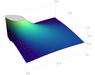
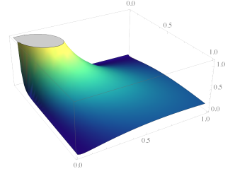
Figure 1: The minimal eigenvalue of the Hessian of the Tsallis-perspective in $d=2$ dimensions (see Eq. 1) of $h=\psi_{\alpha}$ (see Eq. 2) with $\alpha=0$ (left) vs. $\alpha=0.25$ (right). The dashed red lines indicate the zero level set. We see that convexity of $\psi_{\alpha}$ is insufficient to ensure that $\Psi_{\alpha}$ is even convex (let alone strongly convex), and the linear shift introduced in $\psi_{\alpha}$ is crucial for this purpose.

Remarkably, however, there is a simple condition on $h$ under which it can be shown that not only $H$ is convex, but in fact admits a strong lower bound over its Hessian. This is detailed in the following lemma.

Lemma 1.

Assume that $h:[0,1]\to\mathbb{R}$ is twice-differentiable, strictly convex and satisfies the following condition for some constants $c_{h}\in\mathbb{R}$ and $\lambda_{h}>0$, for all vectors $y\in Y\subseteq\mathcal{S}_{d}$:

$$\sum_{i=1}^{d}h(y_{i})+2\sum_{i=1}^{d}\frac{\brk!{h^{\prime}(y_{i})-c_{h}}^{2}}{h^{\prime\prime}(y_{i})}+\lambda_{h}\leq 0.$$

Then, at any $x\in\mathbb{R}^{d}_{+}$ such that $x/\norm{x}_{1}\in Y$, the function $H$ satisfies

$$\nabla^{2}H(x)\succeq\frac{\lambda_{h}}{4}\norm{x}_{1}^{-\frac{3}{2}}J+\frac{1}{2}\norm{x}_{1}^{-\frac{7}{2}}\sum_{i=1}^{d}x_{i}^{2}h^{\prime\prime}\brk 2{\frac{x_{i}}{\norm{x}_{1}}}z_{i}z_{i}^{\mathsf{T}},$$

where $J$ is the $d$-by-$d$ all-ones matrix and $z_{i}=\mathbf{1}_{d}-\brk{\norm{x}_{1}/x_{i}}\mathbf{e}_{i}$ for $i\in[d]$.

Proof.

Fix $x\in\mathbb{R}^{d}_{+}$ and let $y_{i}=x_{i}/\norm{x}_{1}$ for all $i$. Using Lemma 6 in Appendix A, the Hessian of $H$ can be written as

$$\nabla^{2}H(x)=\frac{1}{4}\norm{x}_{1}^{-\tfrac{3}{2}}\sum_{i=1}^{d}\brk 2{-h(y_{i})zz^{\mathsf{T}}+4y_{i}^{2}h^{\prime\prime}(y_{i})z_{i}z_{i}^{\mathsf{T}}+2y_{i}h^{\prime}(y_{i})\brk!{zz_{i}^{\mathsf{T}}+z_{i}z^{\mathsf{T}}}},$$

where $z=\mathbf{1}_{d}$ is the all-ones vector, and $z_{i}=\mathbf{1}_{d}-\brk{\norm{x}_{1}/x_{i}}\mathbf{e}_{i}$ for all $i\in[d]$. Then, using the condition on $h$ and since $\sum_{i=1}^{d}y_{i}z_{i}=0$ we have

$$\nabla^{2}H(x)$$

$$\succeq\frac{\lambda_{h}}{4}\norm{x}_{1}^{-\tfrac{3}{2}}J+\frac{1}{4}\norm{x}_{1}^{-\tfrac{3}{2}}\sum_{i=1}^{d}\brk*{\frac{\brk!{h^{\prime}(y_{i})-c_{h}}^{2}}{\frac{1}{2}h^{\prime\prime}(y_{i})}zz^{\mathsf{T}}+4y_{i}^{2}h^{\prime\prime}\brk{y_{i}}z_{i}z_{i}^{\mathsf{T}}+2y_{i}h^{\prime}\brk{y_{i}}\brk!{zz_{i}^{\mathsf{T}}+z_{i}z^{\mathsf{T}}}}$$

$$=\frac{\lambda_{h}}{4}\norm{x}_{1}^{-\tfrac{3}{2}}J+\frac{1}{4}\norm{x}_{1}^{-\tfrac{3}{2}}\sum_{i=1}^{d}\brk*{\frac{\brk!{h^{\prime}(y_{i})-c_{h}}^{2}}{\frac{1}{2}h^{\prime\prime}(y_{i})}zz^{\mathsf{T}}+4y_{i}^{2}h^{\prime\prime}\brk{y_{i}}z_{i}z_{i}^{\mathsf{T}}+2y_{i}(h^{\prime}\brk{y_{i}}-c_{h})\brk!{zz_{i}^{\mathsf{T}}+z_{i}z^{\mathsf{T}}}}$$

$$=\frac{\lambda_{h}}{4}\norm{x}_{1}^{-\tfrac{3}{2}}J+\frac{1}{4}\norm{x}_{1}^{-\tfrac{3}{2}}\sum_{i=1}^{d}\brk 4{\frac{h^{\prime}(y_{i})-c_{h}}{\sqrt{\frac{1}{2}h^{\prime\prime}(y_{i})}}z+2y_{i}\sqrt{\tfrac{1}{2}h^{\prime\prime}(y_{i})}z_{i}}\brk 4{\frac{h^{\prime}(y_{i})-c_{h}}{\sqrt{\frac{1}{2}h^{\prime\prime}(y_{i})}}z+2y_{i}\sqrt{\tfrac{1}{2}h^{\prime\prime}(y_{i})}z_{i}}^{\mathsf{T}}$$

$$\quad+\frac{\lambda_{h}}{4}\norm{x}_{1}^{-\tfrac{3}{2}}\sum_{i=1}^{d}y_{i}^{2}h^{\prime\prime}(y_{i})z_{i}z_{i}^{\mathsf{T}},$$

and the result follows since each term in the first summation is psd. ∎

3.2 Deriving the Tsallis-Shannon entropy

We can now define the Tsallis-Shannon entropy in terms of Tsallis-perspectives and derive its local strong convexity properties that we require for our analysis. For a given $\alpha>0$, the Tsallis-Shannon entropy with respect to a partition $V_{1},\ldots,V_{K}$ of $V=[N]$ is defined for all $p\in\mathbb{R}^{d}_{+}$ as

$$\Psi_{\alpha}(p)=\sum_{k=1}^{K}\sqrt{p(V_{k})}\cdot\sum_{i\in V_{k}}\psi_{\alpha}\brk 3{\frac{p_{i}}{p(V_{k})}}~{},\quad\text{where}\quad\psi_{\alpha}(y)=y\log y-\alpha y~{}.$$ (2)

Namely, $\Psi_{\alpha}$ is the sum of the Tsallis-perspectives of $\psi_{\alpha}$ with respect to each partition element $V_{k}$. Observe that $\psi_{\alpha}$ corresponds to a single term of a (linearly shifted) negative Shannon entropy. Thus, for a probability vector $p$, the function $\Psi_{\alpha}$ can be viewed as a bi-level entropy, where the top level amounts to the marginal probabilities $p(V_{k})$ (for $k\in[K]$) and the bottom level to the conditional probabilities $p_{i}/p(V_{k})$ (for $i\in V_{k}$); for the marginal probabilities $\Psi_{\alpha}$ behaves like a $\tfrac{1}{2}$-Tsallis entropy, while on the conditional probabilities it operates as a (negative, shifted) Shannon entropy.

It is not hard to show that the magnitude of $\Psi_{\alpha}(p)$ is at most $\mathcal{O}(\sqrt{K}\log{N})$, which is crucial for our purposes as it avoids a direct polynomial dependence on the dimension $N$. On the other hand, using Lemma 1, we can prove the following lower bound for the Hessian of $\Psi_{\alpha}$ for an appropriate choice of $\alpha$. We remark that the setting of $\alpha$ is crucial: the linear shift in the Shannon entropy component is essential even just for ensuring the convexity of $\Psi_{\alpha}$ (see Fig. 1).

Lemma 2.

Fix $\gamma>0$, and let $p\in\mathbb{R}^{N}_{+}$ such that $p_{i}/p(V_{k})\geq\gamma$ for all $i,k$ with $i\in V_{k}$. Then for $\alpha=2\brk{1+\log^{2}(\ifrac{1}{\gamma})}$, the Hessian of $\Psi_{\alpha}$ at $p$ satisfies

$$\nabla^{2}\Psi_{\alpha}(p)\succeq\frac{1}{2}\operatorname{diag}\brk*{\frac{1}{p_{1}\sqrt{p(V(1))}},\frac{1}{p_{2}\sqrt{p(V(2))}},\ldots,\frac{1}{p_{N}\sqrt{p(V(N))}}}.$$

Proof.

For brevity, we omit all $\alpha$ subscripts below. Observe that $\Psi$ is a separable sum of $K$ functions, each of which is a function of variables $p_{i}$ with $i\in V_{k}$, thus its Hessian $\nabla^{2}\Psi(p)$ is block-diagonal with blocks aligned with $V_{1},\ldots,V_{K}$. It therefore suffices to establish the Hessian bound for a function of the form $\Psi^{\circ}(x)=\sqrt{\norm{x}_{1}}\sum_{i=1}^{d}\psi\brk{\ifrac{x_{i}}{\norm{x}_{1}}}$ corresponding to a set of variables $V=\set{x_{1},\ldots,x_{d}}$. To this end, we first show that the function $\psi$ satisfies the conditions of Lemma 1 over the domain $Y=\mathcal{S}_{d}\cap\set{y:y_{i}\geq\gamma,~{}\forall~{}i\in[d]}$, with constants $c_{\psi}=-\brk{1+2\log^{2}(\ifrac{1}{\gamma})}$ and $\lambda_{\psi}=2$. Indeed, twice differentiability and strict convexity are immediate, and for any $y\in Y$ we have

$$\sum_{i=1}^{d}\psi(y_{i})+2\sum_{i=1}^{d}\frac{\brk!{\psi^{\prime}(y_{i})-c_{\psi}}^{2}}{\psi^{\prime\prime}(y_{i})}+\lambda_{\psi} \leq-2\log^{2}\tfrac{1}{\gamma}+2\sum_{i=1}^{d}y_{i}\brk!{\log y_{i}-1-2\log^{2}\tfrac{1}{\gamma}-c_{\psi}}^{2}$$

$$=-2\log^{2}\tfrac{1}{\gamma}+2\sum_{i=1}^{d}y_{i}\log^{2}y_{i}$$

$$\leq 0.$$

Applying the latter lemma on $\Psi^{\circ}$, we obtain (below $J$ denotes the $d$-by-$d$ all-ones matrix):

$$\nabla^{2}\Psi^{\circ}(x) \succeq\frac{1}{2}\norm{x}_{1}^{-\frac{3}{2}}J+\frac{1}{2}\norm{x}_{1}^{-\frac{7}{2}}\sum_{i=1}^{d}x_{i}^{2}\psi^{\prime\prime}\brk 2{\frac{x_{i}}{\norm{x}_{1}}}z_{i}z_{i}^{\mathsf{T}}$$

$$=\frac{1}{2}\norm{x}_{1}^{-\frac{3}{2}}J+\frac{1}{2}\norm{x}_{1}^{-\frac{5}{2}}\sum_{i=1}^{d}x_{i}z_{i}z_{i}^{\mathsf{T}}$$

$$=\frac{1}{2}\norm{x}_{1}^{-\frac{3}{2}}J+\frac{1}{2}\norm{x}_{1}^{-\frac{3}{2}}J-\frac{1}{2}\norm{x}_{1}^{-\frac{3}{2}}\sum_{i=1}^{d}\brk!{\mathbf{1}_{d}\mathbf{e}_{i}^{\mathsf{T}}+\mathbf{e}_{i}\mathbf{1}_{d}^{\mathsf{T}}}+\frac{1}{2}\norm{x}_{1}^{-\frac{1}{2}}\sum_{i=1}^{d}\frac{1}{x_{i}}\mathbf{e}_{i}\mathbf{e}_{i}^{\mathsf{T}}$$

$$=\norm{x}_{1}^{-\frac{3}{2}}J-\frac{1}{2}\norm{x}_{1}^{-\frac{3}{2}}\brk*{2J}+\frac{1}{2}\norm{x}_{1}^{-\frac{1}{2}}\operatorname{diag}{\brk*{\frac{1}{x_{1}},\frac{1}{x_{2}},...,\frac{1}{x_{d}}}}$$

$$=\frac{1}{2\sqrt{\norm{x}_{1}}}\operatorname{diag}{\brk*{\frac{1}{x_{1}},\frac{1}{x_{2}},...,\frac{1}{x_{d}}}},$$

and the result follows. ∎

4 Algorithm and Main Result

In this section we present our best-of-all-worlds algorithm for online learning with feedback graphs. The algorithm, detailed in Algorithm 1, follows the general Follow-the-Regularized-Leader (FTRL) template, and is instantiated by a choice of time-varying convex regularization functions $R_{t}$ together with a standard loss estimator for graph-structured feedback due to Alon et al. (2017).

Input: clique covering $\brk[c]*{V_{1},V_{2},...,V_{K}}$ of an undirected feedback graph $G$;

let $\alpha=2\brk{\log^{2}(NT)+1}$, $\beta=9$, $\gamma=\ifrac{1}{(NT)}$, and step sizes $\eta_{t}=\ifrac{1}{\sqrt{t}}$;

initialize $\widehat{L}_{0,i}=0$ for all $i\in[N]$;

for $t=1,2,...,T$ do

       update

$$p_{t}=\operatorname{arg\,min}_{p\in\mathcal{S}^{\gamma}_{N}}\set!{\widehat{L}_{t-1}\boldsymbol{\cdot}p+R_{t}(p)}$$

where $R_{t}(p)=\eta_{t}^{-1}\Psi(p)+\Phi(p)$ ($\Psi$ and $\Phi$ are defined in Eqs. 3 and 4);

pick arm $I_{t}\sim p_{t}$, observe feedback $\set!{(i,\ell_{t,i}):i\in\mathcal{N}(I_{t})}$ and set

    $$\forall i\in [N]:{\widehat{\mathrm{\ell }}}_{t,i}=\frac{{\mathrm{\ell }}_{t,i}}{p_t(V(i))}𝕀\{i\in V(I_t)\}\text{;}$$

       update $\widehat{L}_{t}=\widehat{L}_{t-1}+\smash{\widehat{\ell}}_{t}$;

      

end for

Algorithm 1 FTRL with feedback graphs

Our main result regarding Algorithm 1 is given in the following.

Theorem 1.

Algorithm 1 attains the following expected pseudo-regret bound in the $C$-corrupted stochastic setting:

$$\mathcal{R}_{T} =\widetilde{\mathcal{O}}\brk 3{\min\brk[c]3{\sqrt{KT},\mathchoice{\sum_{\mathclap{k:\Delta_{k}>0}}\;}{\sum_{k:\Delta_{k}>0}}{\sum_{k:\Delta_{k}>0}}{\sum_{k:\Delta_{k}>0}}\ifrac{1}{\Delta_{k}}+\sqrt{C\,\mathchoice{\sum_{\mathclap{k:\Delta_{k}>0}}\;}{\sum_{k:\Delta_{k}>0}}{\sum_{k:\Delta_{k}>0}}{\sum_{k:\Delta_{k}>0}}\ifrac{1}{\Delta_{k}}}}}.$$

The regularizer $R_{t}$ is formed as a sum of two convex functions, $\Psi$ and $\Phi$, described below. Predictions are computed by the algorithm by minimizing the cumulative estimated loss, regularized by $R_{t}$, over a truncated simplex $\mathcal{S}^{\gamma}_{N}\triangleq\brk[c]{p\in\mathcal{S}_{N}:\forall i,~{}p_{i}\geq\gamma}.$ For loss estimation, the algorithm relies on the standard unbiased loss estimators (denoted by $\smash{\widehat{\ell}}_{t}$) for the graph-feedback framework. Note however that the while feedback the algorithm revealed at time step $t$ includes the losses of all the neighbors of $I_{t}$ in $G$, it only makes use of the losses of the arms which belong to the same clique as $I_{t}$; in other words, the algorithm may ignore some of the feedback it receives.

The primary regularization function $\Psi$ (whose weight increases with time) is the Tsallis-Shannon entropy $\Psi_{\alpha}$ defined in Section 3, given explicitly as

$$\Psi(p)=-\alpha\sum_{k=1}^{K}\sqrt{p(V_{k})}+\sum_{k=1}^{K}\frac{1}{\sqrt{p(V_{k})}}\sum_{i\in V_{k}}p_{i}\log\frac{p_{i}}{p(V_{k})}.$$ (3)

The second time-invariant regularizer $\Phi$ is a log-barrier of the marginal clique probabilities,

$$\Phi(p)=-\beta\sum_{k=1}^{K}\log p(V_{k}),$$ (4)

and its goal is to further stabilize the algorithm. While the idea of augmenting the regularizer with a log-barrier function for promoting stability is not new, we note that a standard log-barrier of the form $-\smash{\sum_{i=1}^{N}}\log p_{i}$ would inevitably introduce an additive $\mathcal{O}(N)$ to the regret, which is suboptimal for our purposes. For that reason we use a different variant of a log-barrier function that operates on the marginal probabilities of the cliques.

5 Proof of Theorem 1

In this section we provide details on the proof of our main theorem. Our main step towards proving Theorem 1 is the following general regret bound for Algorithm 1.

Theorem 2.

Algorithm 1 attains the following pseudo-regret bound, regardless of the corruption level:

$$\mathcal{R}_{T}=\widetilde{\mathcal{O}}\brk*{K+\sum_{t=1}^{T}\mathchoice{\sum_{\mathclap{k\neq k^{\star}}}}{\sum_{k\neq k^{\star}}}{\sum_{k\neq k^{\star}}}{\sum_{k\neq k^{\star}}}\sqrt{\frac{\mathbb{E}\brk[s]*{p_{t}(V_{k})}}{t}}+\sum_{t=1}^{T}\sqrt{\frac{\mathbb{E}[p_{t}\brk*{V_{k^{\star}}\!\setminus\!i^{\star}}]}{t}}+\sum_{t=1}^{T}\sqrt{\frac{\mathbb{E}[p_{t}^{+}\brk*{V_{k^{\star}}\!\setminus\!{i^{\star}}}]}{t}}},$$ (5)

where $p_{t}^{+}=\operatorname{arg\,min}_{p\in\mathcal{S}^{\gamma}_{N}}\set{\widehat{L}_{t}\boldsymbol{\cdot}p+R_{t}(p)}$ for all $t$.

The focus of this section is on proving Theorem 2, but first we sketch how it implies our main result.

Proof of Theorem 1 (sketch; full proof in Section B.5).

The worst-case bound of $\widetilde{\mathcal{O}}\brk{\sqrt{KT}}$ follows immediately from the fact that $\sum_{t=1}^{T}\sum_{k=1}^{K}\sqrt{\mathbb{E}[p_{t}(V_{k})]/t}\leq 2\sqrt{KT}$ via Jensen’s inequality, and similarly for the term including $p_{t}^{+}$. The bound involving the corruption level $C$ requires a more delicate argument due to Zimmert and Seldin (2019) that makes use of a self-bounding property of the pseudo-regret. In more detail, using Young’s inequality one has for all $z>0$:

$$\sum_{t=1}^{T}\mathchoice{\sum_{\mathclap{k\neq k^{\star}}}}{\sum_{k\neq k^{\star}}}{\sum_{k\neq k^{\star}}}{\sum_{k\neq k^{\star}}}\sqrt{\frac{\mathbb{E}[p_{t}(V_{k})]}{t}} \leq\sum_{t=1}^{T}\mathchoice{\sum_{\mathclap{k\neq k^{\star}}}}{\sum_{k\neq k^{\star}}}{\sum_{k\neq k^{\star}}}{\sum_{k\neq k^{\star}}}\brk*{\ifrac{z}{2t\Delta_{k}}+\ifrac{\mathbb{E}[p_{t}(V_{k})]\Delta_{k}}{2z}},$$

and a similar bound can be shown for the other two summations in Eq. 5. Combining these two gives after some simplification the pseudo-regret bound $\mathcal{R}_{T}\leq zB+z^{-1}(\mathcal{R}_{T}+2C),$ for $B=\mathcal{O}\brk{\mathchoice{\sum_{\mathclap{k:\Delta_{k}>0}}\;}{\sum_{k:\Delta_{k}>0}}{\sum_{k:\Delta_{k}>0}}{\sum_{k:\Delta_{k}>0}}\ifrac{\log(T)}{\Delta_{k}}}$, which further simplifies to $\mathcal{R}_{T}\leq 2B+(z-1)B+\frac{2C+B}{z-1}$. Optimizing the bound with respect to $z$ then gives $\mathcal{R}_{T}\leq 4B+4\sqrt{BC},$ which implies the bound we claimed. ∎

We now set to prove Theorem 2. Our starting point is a general regret bound for FTRL. Applying a variation on the standard FTRL analysis (a similar analysis was used in Zimmert and Seldin (2019); Jin and Luo (2020)) to the FTRL instance of Algorithm 1 gives the following regret bound.

Lemma 3.

For all $p^{\gamma}\in\mathcal{S}^{\gamma}_{N}$ the following holds:

$$\sum_{t=1}^{T}\smash{\widehat{\ell}}_{t}\cdot\brk*{p_{t}-p^{\gamma}} \leq\Phi(p^{\gamma})-\Phi(p_{1})+\sum_{t=1}^{T}\brk*{\frac{1}{\eta_{t}}-\frac{1}{\eta_{t-1}}}\brk*{\Psi(p^{\gamma})-\Psi(p_{t})}$$ (6)

$$+2\sum_{t=1}^{T}\eta_{t}\brk*{\norm{\smash{\widehat{\ell}}_{t}-\ell_{t,i^{\star}}\mathbf{1}}_{t}^{*}}^{2}.$$ (7)

Here $\norm{g}_{t}^{*}=\sqrt{g^{\mathsf{T}}(\nabla^{2}\Psi(\tilde{p}_{t}))^{-1}g}$ is the dual local norm induced by $\Psi$ at $\tilde{p}_{t}$ for some intermediate point $\tilde{p}_{t}\in[p_{t},p_{t}^{+}]$, where $p_{t}^{+}=\operatorname{arg\,min}_{p\in\mathcal{S}^{\gamma}_{N}}\set{\widehat{L}_{t}\boldsymbol{\cdot}p+R_{t}(p)}$.

For the proof, see Appendix C. The bound above can be seen as a sum of a penalty term and a stability term (RHS of Eqs. 6 and 7 respectively). In order to prove Theorem 2 using this general regret bound, we separately bound the penalty and stability terms. The penalty term is simpler to handle, and we only provide a brief discussion about how it is bounded. Bounding the stability term requires more work and constitutes the bulk of our analysis and our main contributions. We remark that the stability term contains dual norms of the loss estimators after introducing an additive shift of the form $\ell_{t,i^{\star}}$ to each arm. The purpose of such a shift is to exclude the contribution of the best arm $i^{\star}$ from the regret bound, as can be seen in Eq. 5. More details regarding this shift and its purpose are given in Section B.2.

Bounding the penalty term:

We present a brief discussion about bounding the penalty term in Eq. 6. The penalty term is handled using bounds on the magnitude of the regularization over the domain $\mathcal{S}^{\gamma}_{N}$.

Lemma 4.

The penalty term (RHS of Eq. 6) is upper bounded by

$$\widetilde{\mathcal{O}}\brk*{K+\sum_{t=1}^{T}\sum_{k\neq k^{\star}}\sqrt{\frac{p_{t}(V_{k})}{t}}+\sum_{t=1}^{T}\sqrt{\frac{p_{t}\brk*{V_{k^{\star}}\setminus i^{\star}}}{t}}},$$

for $p^{\gamma}$ defined by $p^{\gamma}_{i}=\begin{cases}\gamma&i\neq i^{\star}\\ 1-(N-1)\gamma&i=i^{\star}\end{cases}.$

Proof (sketch; full proof in Section B.3).

Essentially, we use the fact that the log-barrier component of the regularization is bounded by $\widetilde{\mathcal{O}}(K)$, and the Tsallis-Shannon component evaluated on the prediction $p_{t}$ is bounded by $\widetilde{\mathcal{O}}\brk!{\sum_{k=1}^{K}\sqrt{p_{t}(V_{k})}}$, as it can be seen as a weighted sum of entropy functions (bounded in magnitude by $\log N$), each of which corresponds to a clique $V_{k}$ with the respective weight being $\sqrt{p_{t}(V_{k})}$. The non-trivial part in bounding the penalty term is in omitting the term corresponding to $V_{k^{\star}}$ from the sum. This is accomplished by our specific choice of $p^{\gamma}$ described above, as well as carefully bounding the (Shannon) entropy terms within each clique. ∎

Bounding the stability term:

The following lemma provides an upper bound on the stability term (RHS of Eq. 7). This lemma crucially relies on strong convexity properties of the Tsallis-Shannon regularization (Eq. 3). These properties allow us to obtain highly non-trivial upper bounds on the eigenvalues of the inverse Hessian of $\Psi(\cdot)$ over $\mathcal{S}^{\gamma}_{N}$, and our ability to obtain such bounds turns out to be critical for us to be able to successfully bound the stability term.

Lemma 5.

The following holds for all time steps $t$:

$$\mathbb{E}\brk[s]!{\brk{\norm{\smash{\widehat{\ell}}_{t}-\ell_{t,i^{\star}}\mathbf{1}}_{t}^{*}}^{2}}=\widetilde{\mathcal{O}}\brk 4{\sum_{k\neq k^{\star}}\sqrt{\mathbb{E}\brk[s]!{p_{t}(V_{k})}}+\sqrt{\mathbb{E}\brk[s]!{p_{t}^{+}\brk*{V_{k^{\star}}\!\setminus\!i^{\star}}}}}.$$

Proof (sketch; full proof in Section B.2).

For simplicity, in this proof sketch we ignore the shift in the loss estimation and only bound $\mathbb{E}\brk[s]{\brk{\norm{\smash{\widehat{\ell}}_{t}}_{t}^{*}}^{2}}$ as it captures the main challenges and new ideas in the analysis. First, recall that the dual norm is formally defined with respect to the Hessian of $\Psi(\cdot)$ at some intermediate point $\tilde{p}_{t}\in[p_{t},p_{t}^{+}]$. We use the stability properties induced by the augmented log-barrier regularizer to replace $\tilde{p}_{t}(V_{i})$ terms with $p_{t}(V_{i})$ up to constant factors, and within each clique, bound the remaining terms involving $\tilde{p}_{i}$ by a sum of similar terms with the latter replaced by $p_{i}$ and $p^{+}_{i}$.

Next, for bounding the relevant dual norm, we require a suitable upper bound on $\smash{\brk{\nabla^{2}\Psi(p_{t})}^{-1}}.$ To this end, we employ Lemma 2, by which $\smash{\nabla^{2}\Psi(p_{t})}$ is lower bounded by a diagonal matrix $D_{t}$, in which the $i$’th diagonal entry corresponding to $i\in V_{k}$ is of the form $\smash{\brk!{2\sqrt{p_{t}(V_{k})}p_{t,i}}^{-1}}.$ We now use this crucial fact to obtain the following upper bound on the stability term:

$$\mathbb{E}\brk[s]!{\brk{\norm{\smash{\widehat{\ell}}_{t}}_{t}^{*}}^{2}}\leq 2\mathbb{E}\brk[s]*{\smash{\widehat{\ell}}_{t}^{\mathsf{T}}D_{t}^{-1}\smash{\widehat{\ell}}_{t}}=2\mathbb{E}\brk[s]*{\sum_{k=1}^{K}\sqrt{p_{t}(V_{k})}\sum_{i\in V_{k}}p_{t,i}\smash{\widehat{\ell}}_{t,i}^{2}}.$$

We keep bounding this term by using the definition of the loss estimators $\smash{\widehat{\ell}}_{t}$ to obtain

$$\mathbb{E}\brk[s]!{\brk{\norm{\smash{\widehat{\ell}}_{t}}_{t}^{*}}^{2}}\leq 2\mathbb{E}\brk[s]*{\sqrt{p_{t}\brk*{V({I_{t}})}}\sum_{\mathclap{i\in V(I_{t})}}p_{t,i}\brk*{\frac{\ell_{t,i}}{p_{t}\brk*{V({I_{t}})}}}^{2}}\leq 2\mathbb{E}\brk[s]*{\frac{1}{\sqrt{p_{t}\brk*{V({I_{t}})}}}}=2\mathbb{E}\brk[s]*{\sum_{k=1}^{K}\sqrt{p_{t}(V_{k})}},$$

where in the last line we used the fact that the probability that at time step $t$ the algorithm chooses an arm from the clique $V_{k}$ is $p_{t}(V_{k})$. Note that this bound contains a term for $p_{t,i^{\star}}$ which we would like to omit from the final bound. As we remarked before, the way we mitigate that is by considering the shifted loss estimators. This is explained in full in Section B.2. ∎

Concluding the proof:

We can now sketch the proof of Theorem 2 using the bounds we obtained. A formal proof that also takes into account the poly-log factors can be found in Section B.4.

Proof of Theorem 2 (sketch; full proof in Section B.4).

We first remark that it suffices to bound the expected regret with respect to $p^{\gamma}$ given by $\mathbb{E}\brk[s]!{\sum_{t=1}^{T}\ell_{t}\cdot\brk*{p_{t}-p^{\gamma}}}$, since it can only be larger than the pseudo-regret by an additive constant, as shown in Section B.4. In addition, since the loss estimators $\smash{\widehat{\ell}}_{t}$ are unbiased estimators of the loss vectors $\ell_{t}$ we conclude that it suffices to bound the regret with respect to the loss estimators, i.e. $\mathbb{E}\brk[s]!{\sum_{t=1}^{T}\smash{\widehat{\ell}}_{t}\cdot\brk*{p_{t}-p^{\gamma}}}$ which is bounded by the sum of the expected penalty and stability terms (Eqs. 6 and 7). Lemma 4 gives a bound on the penalty term of the form

$$\widetilde{\mathcal{O}}\brk*{K+\sum_{t=1}^{T}\sum_{k\neq k^{\star}}\sqrt{\ifrac{\mathbb{E}[p_{t}(V_{k})]}{t}}+\sum_{t=1}^{T}\sqrt{\ifrac{\mathbb{E}[p_{t}\brk*{V_{k^{\star}}\!\setminus\!i^{\star}}]}{t}}},$$

and Lemma 5 gives a bound on the stability term of the form

$$\widetilde{\mathcal{O}}\brk*{\sum_{t=1}^{T}\sum_{k\neq k^{\star}}\sqrt{\ifrac{\mathbb{E}[p_{t}(V_{k})]}{t}}+\sum_{t=1}^{T}\sqrt{\ifrac{p_{t}^{+}\brk*{V_{k^{\star}}\!\setminus\!{i^{\star}}}}{t}}}.$$

Adding the two bounds and rearranging, we conclude the proof of Theorem 2. ∎

Acknowledgements

This work has received support from the Israeli Science Foundation (ISF) grant no. 2549/19, from the Len Blavatnik and the Blavatnik Family foundation, and from the Yandex Initiative in Machine Learning.

Appendix A Tsallis-perspective: Technical Proofs

To prove Lemma 1 we need the following technical result that gives an expression for the Hessian of the Tsallis-perspective $H$ in terms of the (scalar) derivatives of $h$.

Lemma 6.

The Hessian of $H$ (Eq. 1) at any point $x\in\mathbb{R}_{+}^{d}$ can be expressed as:

$$\nabla^{2}H(x)= -\frac{1}{4}\norm{x}_{1}^{-\tfrac{3}{2}}\sum_{i=1}^{d}h\brk 2{\frac{x_{i}}{\norm{x}_{1}}}zz^{\mathsf{T}}$$

$$+\norm{x}_{1}^{-\tfrac{7}{2}}\sum_{i=1}^{d}x_{i}^{2}h^{\prime\prime}\brk 2{\frac{x_{i}}{\norm{x}_{1}}}z_{i}z_{i}^{\mathsf{T}}$$

$$+\frac{1}{2}\norm{x}_{1}^{-\tfrac{5}{2}}\sum_{i=1}^{d}x_{i}h^{\prime}\brk 2{\frac{x_{i}}{\norm{x}_{1}}}\brk!{zz_{i}^{\mathsf{T}}+z_{i}z^{\mathsf{T}}}~{},$$

where $z=\mathbf{1}_{d}$ is the all-ones vector, and $z_{i}=\mathbf{1}_{d}-(\norm{x}_{1}/x_{i})\mathbf{e}_{i}$ for all $i\in[d]$.

Proof.

Let us first compute the first and second derivatives of $f(x)=\sqrt{\norm{x}_{1}}$ and $g_{i}(x)=h\brk{\ifrac{x_{i}}{\norm{x}_{1}}}$ for a fixed $i\in[d]$:

$$\nabla f(x) =\frac{1}{2}\norm{x}_{1}^{-\tfrac{1}{2}}z;$$

$$\nabla^{2}f(x) =-\frac{1}{4}\norm{x}_{1}^{-\tfrac{3}{2}}zz^{\mathsf{T}};$$

$$\nabla g_{i}(x) =h^{\prime}\brk 2{\frac{x_{i}}{\norm{x}_{1}}}\brk 2{\frac{1}{\norm{x}_{1}}\mathbf{e}_{i}-\frac{x_{i}}{\norm{x}_{1}^{2}}z}$$

$$=-\frac{x_{i}}{\norm{x}_{1}^{2}}h^{\prime}\brk 2{\frac{x_{i}}{\norm{x}_{1}}}z_{i};$$

$$\nabla^{2}g_{i}(x) =h^{\prime\prime}\brk 2{\frac{x_{i}}{\norm{x}_{1}}}\brk 2{\frac{1}{\norm{x}_{1}}\mathbf{e}_{i}-\frac{x_{i}}{\norm{x}_{1}^{2}}z}\brk 2{\frac{1}{\norm{x}_{1}}\mathbf{e}_{i}-\frac{x_{i}}{\norm{x}_{1}^{2}}z}^{\mathsf{T}}$$

$$\quad+h^{\prime}\brk 2{\frac{x_{i}}{\norm{x}_{1}}}\brk 2{-\frac{1}{\norm{x}_{1}^{2}}z\mathbf{e}_{i}^{\mathsf{T}}-\frac{1}{\norm{x}_{1}^{2}}\mathbf{e}_{i}z^{\mathsf{T}}+\frac{2x_{i}}{\norm{x}_{1}^{3}}zz^{\mathsf{T}}}$$

$$=\frac{x_{i}^{2}}{\norm{x}_{1}^{4}}h^{\prime\prime}\brk 2{\frac{x_{i}}{\norm{x}_{1}}}z_{i}z_{i}^{\mathsf{T}}+\frac{x_{i}}{\norm{x}_{1}^{3}}h^{\prime}\brk 2{\frac{x_{i}}{\norm{x}_{1}}}\brk{zz_{i}^{\mathsf{T}}+z_{i}z^{\mathsf{T}}}.$$

Using the formula for the Hessian of a product, we now obtain:

$$\mkern-36.0mu\nabla^{2}\brk!{f(x)g_{i}(x)}$$

$$=\brk!{\nabla^{2}f(x)}g_{i}(x)+\nabla f(x)\nabla g_{i}(x)^{\mathsf{T}}+\nabla g_{i}(x)\nabla f(x)^{\mathsf{T}}+f(x)\brk!{\nabla^{2}g_{i}(x)}$$

$$=-\frac{1}{4}\norm{x}_{1}^{-\tfrac{3}{2}}h\brk 2{\frac{x_{i}}{\norm{x}_{1}}}zz^{\mathsf{T}}-\frac{1}{2}\norm{x}_{1}^{-\tfrac{5}{2}}x_{i}h^{\prime}\brk 2{\frac{x_{i}}{\norm{x}_{1}}}\brk!{zz_{i}^{\mathsf{T}}+z_{i}z^{\mathsf{T}}}$$

$$\phantom{=}+\norm{x}_{1}^{-\tfrac{7}{2}}x_{i}^{2}h^{\prime\prime}\brk 2{\frac{x_{i}}{\norm{x}_{1}}}z_{i}z_{i}^{\mathsf{T}}+\norm{x}_{1}^{-\tfrac{5}{2}}x_{i}h^{\prime}\brk 2{\frac{x_{i}}{\norm{x}_{1}}}\brk{zz_{i}^{\mathsf{T}}+z_{i}z^{\mathsf{T}}}$$

$$=-\frac{1}{4}\norm{x}_{1}^{-\tfrac{3}{2}}h\brk 2{\frac{x_{i}}{\norm{x}_{1}}}zz^{\mathsf{T}}+\norm{x}_{1}^{-\tfrac{7}{2}}x_{i}^{2}h^{\prime\prime}\brk 2{\frac{x_{i}}{\norm{x}_{1}}}z_{i}z_{i}^{\mathsf{T}}+\frac{1}{2}\norm{x}_{1}^{-\tfrac{5}{2}}x_{i}h^{\prime}\brk 2{\frac{x_{i}}{\norm{x}_{1}}}\brk!{zz_{i}^{\mathsf{T}}+z_{i}z^{\mathsf{T}}}.$$

Summing this over $i=1,\ldots,d$, we obtain the expression for the Hessian $\nabla^{2}H(x)$. ∎

Appendix B Proof of Main Result

In this section we provide the proof of Theorem 1. In Section B.1 we prove useful lemmas which provide us with stability properties of the FTRL iterates. In Section B.2 and Section B.3 we bound the stability and penalty terms (RHS of Eq. 7 and Eq. 6) towards proving Theorem 2 in Section B.4. We then prove Theorem 1 in Section B.5.

B.1 Stability of Iterates

We first establish a technical stability property of the FTRL updates that is crucial for bounding the stability term (Eq. 7). This property asserts that for every time step $t$, the clique marginal probabilities induced by $p_{t}$ are close, up to a constant multiplicative factor, to the clique marginals induced by $p_{t}^{+}$, where $p_{t}^{+}\triangleq\operatorname{arg\,min}_{p\in\mathcal{S}^{\gamma}_{N}}\set{\widehat{L}_{t}\cdot p+R_{t}(p)}$. The proof uses properties of the log-barrier component $\Phi$, and relies on an adaptation of an argument of Jin and Luo (2020).

Lemma 7.

For all time steps $t$ and cliques $V_{k}$ it holds that $p_{t}^{+}(V_{k})\leq\tfrac{7}{3}p_{t}(V_{k}),$ where $p_{t}^{+}\triangleq\operatorname{arg\,min}_{p\in\mathcal{S}^{\gamma}_{N}}\brk[c]!{\widehat{L}_{t}\cdot p+R_{t}(p)}.$

Proof.

We define:

$$F_{t}(p) =\widehat{L}_{t-1}\cdot p+R_{t}(p),$$

$$F_{t}^{+}(p) =\widehat{L}_{t}\cdot p+R_{t}(p),$$

so that $p_{t}=\operatorname{arg\,min}_{p\in\mathcal{S}^{\gamma}_{N}}\brk[c]*{F_{t}(p)}$ and $p_{t}^{+}=\operatorname{arg\,min}_{p\in\mathcal{S}^{\gamma}_{N}}\brk[c]*{F_{t}^{+}(p)}$. Note that $\nabla^{2}\Phi(p)$ is a block diagonal matrix, with the block corresponding to the clique $V_{k}$ being exactly $\frac{9}{p(V_{k})^{2}}J_{V_{k}}$ where $J_{V_{k}}$ is the $|V_{k}|\times|V_{k}|$ all-ones matrix. A straightforward calculation then shows that for all $p,p^{\prime},p^{\prime\prime}\in\mathcal{S}_{N}$ it holds that:

$$\norm{p^{\prime}-p^{\prime\prime}}_{\nabla^{2}\Phi(p)}^{2}=9\sum_{k=1}^{K}\frac{(p^{\prime}(V_{k})-p^{\prime\prime}(V_{k}))^{2}}{p(V_{k})^{2}}.$$

It suffices to prove that $\norm{p_{t}^{+}-p_{t}}_{\nabla^{2}\Phi(p_{t})}^{2}\leq 16$. This is because by the calculation we just made, we have $\brk*{p_{t}^{+}(V_{k})-p_{t}(V_{k})}^{2}\leq\brk{\frac{4}{3}p_{t}(V_{k})}^{2}$ which is want we want to prove. It then suffices to show that for any $p^{\prime}\in\mathcal{S}^{\gamma}_{N}$ with $\norm{p^{\prime}-p_{t}}_{\nabla^{2}\Phi(p_{t})}^{2}=16$ we have $F_{t}^{+}(p^{\prime})\geq F_{t}^{+}(p_{t})$. This is because as an implication of that, $p_{t}^{+}$ which minimizes the convex function $F_{t}^{+}$, must be within the convex set $\brk[c]!{p:\norm{p-p_{t}}_{\nabla^{2}\Phi(p_{t})}^{2}\leq 16}$. We proceed to lower bound $F_{t}^{+}(p^{\prime})$ as follows:

$$F_{t}^{+}(p^{\prime}) =F_{t}^{+}(p_{t})+\nabla F_{t}^{+}(p_{t})^{\mathsf{T}}(p^{\prime}-p_{t})+\frac{1}{2}\norm{p^{\prime}-p_{t}}_{\nabla^{2}R_{t}(\xi)}^{2}$$

$$=F_{t}^{+}(p_{t})+\nabla F_{t}(p_{t})^{\mathsf{T}}(p^{\prime}-p_{t})+\smash{\widehat{\ell}}_{t}^{\mathsf{T}}(p^{\prime}-p_{t})+\frac{1}{2}\norm{p^{\prime}-p_{t}}_{\nabla^{2}R_{t}(\xi)}^{2}$$

$$\geq F_{t}^{+}(p_{t})+\smash{\widehat{\ell}}_{t}^{\mathsf{T}}(p^{\prime}-p_{t})+\frac{1}{2}\norm{p^{\prime}-p_{t}}_{\nabla^{2}\Phi(\xi)}^{2},$$

where the first equality is a Taylor expansion of $F_{t}^{+}$ around $p_{t}$, with $\xi$ being a point between $p^{\prime}$ and $p_{t}$, and the last inequality is due to first-order optimality conditions and the fact that $\nabla^{2}R_{t}(\xi)\succeq\nabla^{2}\Phi(\xi)$ since $\Psi$ is convex. Note that since $\norm{p^{\prime}-p_{t}}_{\nabla^{2}\Phi(p_{t})}^{2}=16$, by the same argument as in the beginning of the proof we conclude that $p^{\prime}(V_{k})\leq\frac{7}{3}p_{t}(V_{k})$. Since $\xi$ lies between $p_{t}$ and $p^{\prime}$ we conclude the same ratio bound for $\xi$. We can thus bound the last term as follows:

$$\frac{1}{2}\norm{p^{\prime}-p_{t}}_{\nabla^{2}\Phi(\xi)}^{2} =\frac{9}{2}\sum_{k=1}^{K}\frac{(p^{\prime}(V_{k})-p_{t}(V_{k}))^{2}}{\brk{\xi(V_{k})}^{2}}$$

$$\geq\frac{9}{2\cdot\brk*{\frac{7}{3}}^{2}}\sum_{k=1}^{K}\frac{(p^{\prime}(V_{k})-p_{t}(V_{k}))^{2}}{p_{t}(V_{k})^{2}}$$

$$=\frac{9}{2\cdot 49}\norm{p^{\prime}-p_{t}}_{\nabla^{2}\Phi(p_{t})}^{2}$$

$$=\frac{72}{49}\geq 1.$$

It now suffices to show that $\smash{\widehat{\ell}}_{t}^{\mathsf{T}}(p^{\prime}-p_{t})\geq-1$; indeed,

$$\smash{\widehat{\ell}}_{t}^{\mathsf{T}}(p^{\prime}-p_{t})=\sum_{i\in V(I_{t})}\frac{\ell_{t,i}}{p_{t}\brk*{V({I_{t}})}}(p^{\prime}_{t,i}-p_{t,i})\geq-\frac{1}{p_{t}\brk*{V({I_{t}})}}\sum_{i\in V(I_{t})}\ell_{t,i}p_{t,i}\geq-1,$$

and the proof is complete. ∎

The following lemma showcases another stability property that relates $p_{t}$ to $p_{t}^{+}$. A corollary of this lemma is that the pseudo-regret of the iterates $p_{t}$ can only be larger than the pseudo-regret of the iterates $p_{t}^{+}$, and it is used in the proof of Theorem 1 in Section B.5.

Lemma 8.

For all time steps $t$ it holds that

$$p_{t}^{+}\cdot\smash{\widehat{\ell}}_{t}\leq p_{t}\cdot\smash{\widehat{\ell}}_{t},$$

where $p_{t}^{+}\triangleq\operatorname{arg\,min}_{p\in\mathcal{S}^{\gamma}_{N}}\brk[c]!{\widehat{L}_{t}\cdot p+R_{t}(p)}.$

Proof.

Since $p_{t}^{+}$ is a minimizer of $\widehat{L}_{t}\cdot p+R_{t}(p)$ and $p_{t}$ is a minimizer of $\widehat{L}_{t-1}\cdot p+R_{t}(p)$, we have:

$$\widehat{L}_{t}\cdot p_{t}^{+}+R_{t}(p_{t}^{+}) \leq\widehat{L}_{t}\cdot p_{t}+R_{t}(p_{t})$$

$$=\widehat{\ell}_{t}\cdot p_{t}+\widehat{L}_{t-1}\cdot p_{t}+R_{t}(p_{t})$$

$$\leq\widehat{\ell}_{t}\cdot p_{t}+\widehat{L}_{t-1}\cdot p_{t}^{+}+R_{t}(p_{t}^{+}),$$

and the claim follows by rearranging terms. ∎

B.2 Proof of Lemma 5 (Stability)

We now restate Lemma 5 which bounds the stability term to include extra constants which appear in the bound.

Lemma 5restated.

The following holds for all time steps $t$:

$$\mathbb{E}\brk[s]*{\brk{\norm{\smash{\widehat{\ell}}_{t}-\ell_{t,i^{\star}}\mathbf{1}}_{t}^{*}}^{2}}=56\sum_{k\neq k^{\star}}\sqrt{\mathbb{E}\brk[s]!{p_{t}(V_{k})}}+8\sqrt{\mathbb{E}\brk[s]!{p_{t}^{+}\brk*{V_{k^{\star}}\setminus i^{\star}}}}.$$

Here $\norm{g}_{t}^{*}=\sqrt{g^{\mathsf{T}}(\nabla^{2}\Psi(\tilde{p}_{t}))^{-1}g}$ is the dual local norm induced by $\Psi$ at $\tilde{p}_{t}$ for some intermediate point $\tilde{p}_{t}\in[p_{t},p_{t}^{+}]$, where $p_{t}^{+}=\operatorname{arg\,min}_{p\in\mathcal{S}^{\gamma}_{N}}\set{\widehat{L}_{t}\boldsymbol{\cdot}p+R_{t}(p)}$.

Proof.

By Lemma 2, $\nabla^{2}\Psi(\tilde{p}_{t})$ is lower bounded by a diagonal matrix $D_{t}$ in which the $i$’th diagonal entry corresponding to $i\in V_{k}$ is $\brk*{2\sqrt{\tilde{p}_{t}(V_{k})}\tilde{p}_{t,i}}^{-1}$. Equivalently it holds that $\brk*{\nabla^{2}\Psi(\tilde{p}_{t})}^{-1}\preceq D_{t}^{-1}$. Using this fact and the fact that $\smash{\widehat{\ell}}_{t,i}=0$ for $i\notin V(I_{t})$ we have

$$\mathbb{E}\left[\brk*{\norm{\smash{\widehat{\ell}}_{t}-\ell_{t,i^{\star}}\mathbf{1}}_{t}^{*}}^{2}\right] =\mathbb{E}\brk[s]*{\brk*{\smash{\widehat{\ell}}_{t}-\ell_{t,i^{\star}}\mathbf{1}}^{\mathsf{T}}\brk*{\nabla^{2}\Psi(\tilde{p}_{t})}^{-1}\brk*{\smash{\widehat{\ell}}_{t}-\ell_{t,i^{\star}}\mathbf{1}}}$$

$$\leq 2\mathbb{E}\left[\sum_{k=1}^{K}\sqrt{\tilde{p}_{t}(V_{k})}\sum_{i\in V_{k}}\tilde{p}_{t,i}\brk*{\smash{\widehat{\ell}}_{t,i}-\ell_{t,i^{\star}}}^{2}\right]$$

$$=2\mathbb{E}\brk[s]*{\sqrt{\tilde{p}_{t}(V(I_{t}))}\sum_{i\in V(I_{t})}\tilde{p}_{t,i}\brk*{\smash{\widehat{\ell}}_{t,i}-\ell_{t,i^{\star}}}^{2}}$$ (8)

$$+2\mathbb{E}\brk[s]*{\sum_{V_{k}\neq V(I_{t})}\sqrt{\tilde{p}_{t}(V_{k})}\sum_{i\in V_{k}}\tilde{p}_{t,i}(\ell_{t,i^{\star}})^{2}},$$ (9)

where in the final equality we split the sum over cliques into a term for $V(I_{t})$ and a sum over the rest of the cliques. We first show that the RHS of Eq. 8 is bounded as follows:

$$\mathbb{E}\brk[s]*{\sqrt{\tilde{p}_{t}(V(I_{t}))}\sum_{i\in V(I_{t})}\tilde{p}_{t,i}\brk*{\smash{\widehat{\ell}}_{t,i}-\ell_{t,i^{\star}}}^{2}} \leq 16\sum_{k\neq k^{\star}}\sqrt{\mathbb{E}[p(V_{k})]}+4\sqrt{\mathbb{E}\brk[s]*{p_{t}^{+}\brk*{V_{k^{\star}}\setminus i^{\star}}}}.$$

Indeed, due to Lemma 7 and the fact that $\tilde{p}_{t}$ lies between $p_{t}$ and $p_{t}^{+}$ it holds that $\tilde{p}_{t}(V_{k})\leq 3p_{t}(V_{k})$ for all $k$. Plugging in the expression for the loss estimator $\smash{\widehat{\ell}}_{t}$ we obtain

$$\mathbb{E}\left[\sqrt{\tilde{p}_{t}\brk*{V(I_{t})}}\sum_{i\in V(I_{t})}\tilde{p}_{t,i}\brk*{\smash{\widehat{\ell}}_{t,i}-\ell_{t,i^{\star}}}^{2}\right] =\mathbb{E}\left[\sqrt{\tilde{p}_{t}\brk*{V(I_{t})}}\sum_{i\in V(I_{t})}\tilde{p}_{t,i}\brk*{\frac{\ell_{t,i}}{p_{t}\brk*{V({I_{t}})}}-\ell_{t,i^{\star}}}^{2}\right]$$

$$\leq 2\mathbb{E}\left[p_{t}\brk*{V({I_{t}})}^{-\tfrac{3}{2}}\sum_{i\in V(I_{t})}\tilde{p}_{t,i}\brk*{\ell_{t,i}-p_{t}\brk*{V({I_{t}})}\ell_{t,i^{\star}}}^{2}\right]$$

$$=2\mathbb{E}\left[\sum_{k=1}^{K}p_{t}(V_{k})^{-\tfrac{1}{2}}\sum_{i\in V_{k}}\tilde{p}_{t,i}\brk*{\ell_{t,i}-p_{t}(V_{k})\ell_{t,i^{\star}}}^{2}\right],$$

where in the last equality we use the law of total expectation and the fact that conditioned on the history up until time step $t$ (including the decision vector $p_{t}$), the probability that $I_{t}$ belongs to the clique $V_{k}$ is exactly $p_{t}(V_{k})$. In more detail:

$$\mathbb{E}\left[p_{t}\brk*{V({I_{t}})}^{-\tfrac{3}{2}}\sum_{i\in V(I_{t})}\tilde{p}_{t,i}\brk*{\ell_{t,i}-p_{t}\brk*{V({I_{t}})}\ell_{t,i^{\star}}}^{2}\right]$$

$$=\mathbb{E}\left[\mathbb{E}_{t}\left[p_{t}\brk*{V({I_{t}})}^{-\tfrac{3}{2}}\sum_{i\in V(I_{t})}\tilde{p}_{t,i}\brk*{\ell_{t,i}-p_{t}\brk*{V({I_{t}})}\ell_{t,i^{\star}}}^{2}\right]\right]$$

$$=\mathbb{E}\brk[s]*{\sum_{k=1}^{K}\Pr[I_{t}\in V_{k}\mid h_{t}]\cdot\mathbb{E}_{t}\brk[s]*{p_{t}(V_{k})^{-\tfrac{3}{2}}\sum_{i\in V_{k}}\tilde{p}_{t,i}\brk*{\ell_{t,i}-p_{t}(V_{k})\ell_{t,i^{\star}}}^{2}}}$$

$$=\mathbb{E}\brk[s]*{\sum_{k=1}^{K}p_{t}(V_{k})\cdot\mathbb{E}_{t}\brk[s]*{p(V_{k})^{-\tfrac{3}{2}}\sum_{i\in V_{k}}\tilde{p}_{t,i}\brk*{\ell_{t,i}-p_{t}(V_{k})\ell_{t,i^{\star}}}^{2}}}$$

$$=\mathbb{E}\brk[s]*{\mathbb{E}_{t}\brk[s]*{\sum_{k=1}^{K}p_{t}(V_{k})^{-\tfrac{1}{2}}\sum_{i\in V_{k}}\tilde{p}_{t,i}\brk*{\ell_{t,i}-p_{t}(V_{k})\ell_{t,i^{\star}}}^{2}}}$$

$$=\mathbb{E}\left[\sum_{k=1}^{K}p_{t}(V_{k})^{-\tfrac{1}{2}}\sum_{i\in V_{k}}\tilde{p}_{t,i}\brk*{\ell_{t,i}-p_{t}(V_{k})\ell_{t,i^{\star}}}^{2}\right],$$

where $h_{t}$ denotes the history up to and including the choice of $p_{t}$ at time step $t$ (not including the choice of $I_{t}$), and in the fourth equality we use linearity of expectation and the fact that $p_{t}(V_{k})$ is constant when conditioned on $h_{t}$. We proceed to bound the above term, while splitting the sum over cliques into a term for $V_{k^{\star}}$ and a sum for all of the other cliques:

$$\mathbb{E}\left[\sum_{k=1}^{K}p_{t}(V_{k})^{-\tfrac{1}{2}}\sum_{i\in V_{k}}\tilde{p}_{t,i}\brk*{\ell_{t,i}-p_{t}(V_{k})\ell_{t,i^{\star}}}^{2}\right]$$

$$\leq\mathbb{E}\left[\sum_{k\neq k^{\star}}p_{t}(V_{k})^{-\tfrac{1}{2}}\tilde{p}_{t}(V_{k})\right]+\mathbb{E}\left[p_{t}(V_{k^{\star}})^{-\tfrac{1}{2}}\brk 3{\sum_{i\in V_{k^{\star}},i\neq i^{\star}}\tilde{p}_{t,i}+\tilde{p}_{t,i^{\star}}\brk*{1-p_{t}(V_{k^{\star}})}^{2}}\right]$$

$$\leq 3\mathbb{E}\left[\sum_{k\neq k^{\star}}\sqrt{p_{t}(V_{k})}\right]+2\mathbb{E}\left[\tilde{p}_{t}(V_{k^{\star}})^{-\tfrac{1}{2}}\tilde{p}_{t}\brk*{V_{k^{\star}}\setminus i^{\star}}\right]+3\mathbb{E}\left[\brk*{1-p_{t}(V_{k^{\star}})}^{2}\right]$$

$$\leq 6\mathbb{E}\left[\sum_{k\neq k^{\star}}\sqrt{p_{t}(V_{k})}\right]+2\mathbb{E}\left[\sqrt{\tilde{p}_{t}\brk*{V_{k^{\star}}\setminus i^{\star}}}\right]$$

$$\leq 8\mathbb{E}\left[\sum_{k\neq k^{\star}}\sqrt{p_{t}(V_{k})}\right]+2\mathbb{E}\left[\sqrt{p_{t}^{+}\brk*{V_{k^{\star}}\!\setminus\!{i^{\star}}}}\right]$$

$$\leq 8\sum_{k\neq k^{\star}}\sqrt{\mathbb{E}[p_{t}(V_{k})]}+2\sqrt{\mathbb{E}\brk[s]*{p_{t}^{+}\brk*{V_{k^{\star}}\!\setminus\!{i^{\star}}}}},$$

where in the last inequality we used Jensen’s inequality. We now proceed to bound the RHS of Eq. 9:

$$\mathbb{E}\left[\sum_{V_{k}\neq V(I_{t})}\sqrt{\tilde{p}_{t}(V_{k})}\sum_{i\in V_{k}}\tilde{p}_{t,i}(\ell_{t,i^{\star}})^{2}\right] \leq\mathbb{E}\left[\sum_{V_{k}\neq V(I_{t})}\tilde{p}_{t}(V_{k})^{\frac{3}{2}}\right]$$

$$\leq 6\mathbb{E}\left[\sum_{V_{k}\neq V(I_{t})}p_{t}(V_{k})^{\frac{3}{2}}\right]$$ (10)

$$=6\mathbb{E}\left[\sum_{k=1}^{K}(1-p_{t}(V_{k}))p_{t}(V_{k})^{\frac{3}{2}}\right]$$ (11)

$$\leq 12\mathbb{E}\left[\sum_{k\neq k^{\star}}\sqrt{p_{t}(V_{k})}\right]$$

$$\leq 12\sum_{k\neq k^{\star}}\sqrt{\mathbb{E}[p_{t}(V_{k})]},$$

where in Eq. 10 we use Lemma 7 and the fact that $\tilde{p}_{t}$ lies between $p_{t}$ and $p_{t}^{+}$, in Eq. 11 we use the fact that the probability of the clique $V_{k}$ not to be chosen at time step $t$ is $1-p_{t}(V_{k})$ and the last line uses Jensen’s inequality. Combining the two bounds, we conclude the proof. ∎

B.3 Proof of Lemma 4 (Penalty)

In this section we restate Lemma 4 which bounds the penalty term to include the extra constants and poly-log factors.

Lemma 4restated.

The penalty term described in the RHS of Eq. 6 is bounded by

$$9K\log\frac{1}{\gamma}+5\log^{2}\frac{1}{\gamma}\sum_{t=1}^{T}\sum_{k\neq k^{\star}}\sqrt{\frac{p_{t}(V_{k})}{t}}+2\log\frac{1}{\gamma}\sum_{t=1}^{T}\sqrt{\frac{p_{t}\brk*{V_{k^{\star}}\setminus i^{\star}}}{t}},$$ (12)

where $p^{\gamma}_{i}=\begin{cases}\gamma&i\neq i^{\star}\\ 1-(N-1)\gamma&i=i^{\star}\end{cases}$ for all $i\in[N]$ and $\frac{1}{\eta_{0}}\triangleq 0$.

Proof.

Noting that $\Phi(\cdot)\geq 0$ we can bound the first term as follows:

$$\Phi(p^{\gamma})-\Phi(p_{1}) \leq\Phi(p^{\gamma})\leq 9K\log\frac{1}{\gamma}.$$

Continuing with the second part of the penalty term, note that by definition of $p^{\gamma}$ we have $p^{\gamma}(V_{k^{\star}})\geq p_{t}(V_{k^{\star}})$ for all $t$. Also note that $\Psi(p^{\gamma})\leq-2\brk*{\log^{2}\frac{1}{\gamma}+1}\sqrt{p^{\gamma}(V_{k^{\star}})}$. We then have

$$\sum_{t=1}^{T}\brk*{\frac{1}{\eta_{t}}-\frac{1}{\eta_{t-1}}}\brk*{\Psi(p^{\gamma})-\Psi(p_{t})} \leq\sum_{t=1}^{T}\brk*{\sqrt{t}-\sqrt{t-1}}\Bigg{(}2\brk*{\log^{2}\frac{1}{\gamma}+1}\sum_{k=1}^{K}\sqrt{p_{t}(V_{k})}$$

$$+\sum_{k=1}^{K}\frac{1}{\sqrt{p_{t}(V_{k})}}\sum_{i\in V_{k}}p_{t,i}\log\frac{p_{t}(V_{k})}{p_{t,i}}-2\brk*{\log^{2}\frac{1}{\gamma}+1}\sqrt{p^{\gamma}(V_{k^{\star}})}\Bigg{)}$$

$$\leq 2\brk*{\log^{2}\frac{1}{\gamma}+1}\sum_{t=1}^{T}\frac{1}{\sqrt{t}}\sum_{k\neq k^{\star}}\sqrt{p_{t}(V_{k})}$$

$$+\log\frac{1}{\gamma}\sum_{t=1}^{T}\frac{1}{\sqrt{t}}\sum_{k\neq k^{\star}}\sqrt{p_{t}(V_{k})}$$

$$+\sum_{t=1}^{T}\frac{1}{\sqrt{t\cdot p_{t}(V_{k^{\star}})}}\sum_{i\in V_{k^{\star}}}p_{t,i}\log\frac{p_{t}(V_{k^{\star}})}{p_{t,i}}$$

$$\leq 5\log^{2}\frac{1}{\gamma}\sum_{t=1}^{T}\frac{1}{\sqrt{t}}\sum_{k\neq k^{\star}}\sqrt{p_{t}(V_{k})}$$

$$+\sum_{t=1}^{T}\frac{1}{\sqrt{t\cdot p_{t}(V_{k^{\star}})}}\sum_{i\in V_{k^{\star}}}p_{t,i}\log\frac{p_{t}(V_{k^{\star}})}{p_{t,i}},$$ (13)

where the second inequality follows from the fact that $\sqrt{t}-\sqrt{t-1}\leq\frac{1}{\sqrt{t}}$ and that $p_{t,i}\geq\gamma$ for all $t$ and $i$. It is left to bound the final term. Using the inequality $\log x\leq x-1$ for all $x>0$ we have

$$\sum_{i\in V_{k^{\star}}}p_{t,i}\log\frac{p_{t}(V_{k^{\star}})}{p_{t,i}} =\sum_{i\in V_{k^{\star}}\setminus i^{\star}}p_{t,i}\log\frac{p_{t}(V_{k^{\star}})}{p_{t,i}}+p_{t,i^{\star}}\log\frac{p_{t}(V_{k^{\star}})}{p_{t,i^{\star}}}$$

$$\leq\log\frac{1}{\gamma}\sum_{i\in V_{k^{\star}}\setminus i^{\star}}p_{t,i}+p_{t,i^{\star}}\brk*{\frac{p_{t}(V_{k^{\star}})}{p_{t,i^{\star}}}-1}$$

$$=\brk*{\log\frac{1}{\gamma}+1}p_{t}\brk*{V_{k^{\star}}\setminus i^{\star}}$$

$$\leq 2\log\frac{1}{\gamma}p_{t}\brk*{V_{k^{\star}}\setminus i^{\star}}.$$

Plugging this bound into Eq. 13 while using the fact that $\frac{p_{t}\brk*{V_{k^{\star}}\setminus i^{\star}}}{\sqrt{p_{t}(V_{k^{\star}})}}\leq\sqrt{p_{t}\brk*{V_{k^{\star}}\setminus i^{\star}}}$ completes the proof. ∎

B.4 Proof of Theorem 2

In order to prove Theorem 2 we make use of the following simple claim which asserts that the pseudo-regret is bounded up to an additive constant factor by the regret with respect to some probability vector in $\mathcal{S}^{\gamma}_{N}$.

Lemma 9.

For all $\gamma\in[0,\frac{1}{N}]$ and $i^{\star}\in[N]$ the following holds:

$$\mathbb{E}\left[\sum_{t=1}^{T}p_{t}\cdot\smash{\widehat{\ell}}_{t}-\mathbf{e}_{i^{\star}}\cdot\sum_{t=1}^{T}\smash{\widehat{\ell}}_{t}\right]\leq\mathbb{E}\left[\sum_{t=1}^{T}p_{t}\cdot\smash{\widehat{\ell}}_{t}-p^{\gamma}\cdot\sum_{t=1}^{T}\smash{\widehat{\ell}}_{t}\right]+\gamma TN,$$

where $p^{\gamma}_{i}=\begin{cases}\gamma&i\neq i^{\star}\\ 1-(N-1)\gamma&i=i^{\star}\end{cases}\quad\forall i\in[N].$

Proof.

Fix $\gamma\in[0,\frac{1}{N}]$ and $i^{\star}\in[N]$. Note that $\mathbf{e}_{i^{\star}}=p^{\gamma}-v$ where $v$ is defined as follows:

$$v_{i}=\begin{cases}\gamma&i\neq i^{\star}\\ -(N-1)\gamma&i=i^{\star}\end{cases}\quad\forall i\in[N].$$

This observation gives us the following:

$$\mathbb{E}\left[\sum_{t=1}^{T}p_{t}\cdot\smash{\widehat{\ell}}_{t}-\mathbf{e}_{i^{\star}}\cdot\sum_{t=1}^{T}\smash{\widehat{\ell}}_{t}\right] =\mathbb{E}\left[\sum_{t=1}^{T}p_{t}\cdot\ell_{t}-\mathbf{e}_{i^{\star}}\cdot\sum_{t=1}^{T}\ell_{t}\right]$$

$$=\mathbb{E}\left[\sum_{t=1}^{T}p_{t}\cdot\ell_{t}-p^{\gamma}\cdot\sum_{t=1}^{T}\ell_{t}\right]+v\cdot\mathbb{E}\left[\sum_{t=1}^{T}\ell_{t}\right]$$

$$=\mathbb{E}\left[\sum_{t=1}^{T}p_{t}\cdot\smash{\widehat{\ell}}_{t}-p^{\gamma}\cdot\sum_{t=1}^{T}\smash{\widehat{\ell}}_{t}\right]+v\cdot\mathbb{E}\left[\sum_{t=1}^{T}\ell_{t}\right],$$

where the first equality is due to the fact that $\smash{\widehat{\ell}}_{t}$ is an unbiased estimator of $\ell_{t}$. We bound the last term using the expression for $v$:

$$v\cdot\sum_{t=1}^{T}\ell_{t}=\sum_{t=1}^{T}\left[\sum_{i\neq i^{\star}}\gamma\ell_{t,i}-(N-1)\gamma\ell_{t,i^{\star}}\right]\leq\gamma TN,$$

where in the last inequality we use the fact that the losses are bounded in $[0,1]$. ∎

We will also make use of general FTRL regret bound given by Theorem 3 (which we prove in Appendix C) together with the stability and penalty bounds shown in the previous sections. Theorem 2 is restated here in the precise form proved below.

Theorem 2restated.

Algorithm 1 attains the following regret bound, regardless of the corruption level, for $NT\geq 3^{11}$:

$$\mathcal{R}_{T} \leq 9K\log(NT)+6\log^{2}(NT)\sum_{t=1}^{T}\mathchoice{\sum_{\mathclap{k\neq k^{\star}}}}{\sum_{k\neq k^{\star}}}{\sum_{k\neq k^{\star}}}{\sum_{k\neq k^{\star}}}\sqrt{\frac{\mathbb{E}\brk[s]*{p_{t}(V_{k})}}{t}}$$

$$+2\log(NT)\sum_{t=1}^{T}\sqrt{\frac{\mathbb{E}[p_{t}(V_{k^{\star}}\setminus i^{\star})]}{t}}+16\sum_{t=1}^{T}\sqrt{\frac{\mathbb{E}[p_{t}^{+}\brk*{V_{k^{\star}}\!\setminus\!{i^{\star}}}]}{t}}.$$ (14)

Proof.

Note that due to Lemma 9 it suffices to bound $\mathbb{E}\brk[s]*{\sum_{t=1}^{T}\brk*{p_{t}-p^{\gamma}}\cdot\smash{\widehat{\ell}}_{t}}$ where $p^{\gamma}$ is defined by

$$p^{\gamma}_{i}=\begin{cases}\gamma&i\neq i^{\star}\\ 1-(N-1)\gamma&i=i^{\star}\end{cases}\quad\forall i\in[N],$$

since it can only be larger than the pseudo-regret by an additive constant. Using Theorem 3 and then bounding the penalty and stability terms using Lemma 4 and Lemma 5 we obtain

$$\mathcal{R}_{T} \leq 9K\log(NT)+\brk*{5\log^{2}(NT)+112}\sum_{t=1}^{T}\sum_{k\neq k^{\star}}\sqrt{\frac{\mathbb{E}[p_{t}(V_{k})]}{t}}$$

$$+2\log(NT)\sum_{t=1}^{T}\sqrt{\frac{\mathbb{E}[p_{t}(V_{k^{\star}}\setminus i^{\star})]}{t}}+16\sum_{t=1}^{T}\sqrt{\frac{\mathbb{E}[p_{t}^{+}\brk*{V_{k^{\star}}\!\setminus\!{i^{\star}}}]}{t}}$$

$$\leq 9K\log(NT)+6\log^{2}(NT)\sum_{t=1}^{T}\sum_{k\neq k^{\star}}\sqrt{\frac{\mathbb{E}[p_{t}(V_{k})]}{t}}$$

$$+2\log(NT)\sum_{t=1}^{T}\sqrt{\frac{\mathbb{E}[p_{t}(V_{k^{\star}}\setminus i^{\star})]}{t}}+16\sum_{t=1}^{T}\sqrt{\frac{\mathbb{E}[p_{t}^{+}\brk*{V_{k^{\star}}\!\setminus\!{i^{\star}}}]}{t}},$$

where the last inequality holds for $NT\geq 3^{11}$. ∎

B.5 Proof of Theorem 1 (Main)

We can now provide a proof of our main result given in Theorem 1, restated here more precisely.

Theorem 1restated.

Algorithm 1 attains the following expected pseudo-regret bound in the $C$-corrupted stochastic setting, for $NT\geq 3^{11}$:

$$\mathcal{R}_{T} \leq 184\log^{2}(NT)\cdot\min\brk[c]*{\sqrt{KT},\log^{2}(NT)\mathchoice{\sum_{\mathclap{k:\Delta_{k}>0}}\;}{\sum_{k:\Delta_{k}>0}}{\sum_{k:\Delta_{k}>0}}{\sum_{k:\Delta_{k}>0}}\ifrac{\log T}{\Delta_{k}}+\sqrt{C\mathchoice{\sum_{\mathclap{k:\Delta_{k}>0}}\;}{\sum_{k:\Delta_{k}>0}}{\sum_{k:\Delta_{k}>0}}{\sum_{k:\Delta_{k}>0}}\ifrac{\log T}{\Delta_{k}}}}.$$

Proof.

We first prove the following:

$$\mathcal{R}_{T}\leq 184\log^{4}(NT)\mathchoice{\sum_{\mathclap{k:\Delta_{k}>0}}\;}{\sum_{k:\Delta_{k}>0}}{\sum_{k:\Delta_{k}>0}}{\sum_{k:\Delta_{k}>0}}\ifrac{\log T}{\Delta_{k}}+28\log^{2}(NT)\sqrt{C\mathchoice{\sum_{\mathclap{k:\Delta_{k}>0}}\;}{\sum_{k:\Delta_{k}>0}}{\sum_{k:\Delta_{k}>0}}{\sum_{k:\Delta_{k}>0}}\ifrac{\log T}{\Delta_{k}}}.$$

We proceed bounding the RHS of Theorem 2. For all $B,z>0$ we have

$$B\sum_{t=1}^{T}\brk*{\sum_{k\neq k^{\star}}\sqrt{\frac{\mathbb{E}[p_{t}(V_{k})]}{t}}+\sqrt{\frac{\mathbb{E}[p_{t}(V_{k^{\star}}\setminus i^{\star})]}{t}}} \leq B^{2}\cdot z\sum_{t=1}^{T}\sum_{k:\Delta_{k}>0}\frac{1}{2t\Delta_{k}}+\frac{1}{2z}\sum_{t=1}^{T}\sum_{i=1}^{N}\mathbb{E}[p_{t,i}]\delta_{i}$$

$$\leq B^{2}\cdot z\mathchoice{\sum_{\mathclap{k:\Delta_{k}>0}}\;}{\sum_{k:\Delta_{k}>0}}{\sum_{k:\Delta_{k}>0}}{\sum_{k:\Delta_{k}>0}}\ifrac{\log T}{\Delta_{k}}+\frac{1}{2z}\sum_{t=1}^{T}\sum_{i=1}^{N}\mathbb{E}[p_{t,i}]\delta_{i}$$

$$\leq B^{2}\cdot z\mathchoice{\sum_{\mathclap{k:\Delta_{k}>0}}\;}{\sum_{k:\Delta_{k}>0}}{\sum_{k:\Delta_{k}>0}}{\sum_{k:\Delta_{k}>0}}\ifrac{\log T}{\Delta_{k}}+\frac{1}{2z}\brk*{\mathcal{R}_{T}+2C},$$ (15)

where the first inequality is due to Young’s inequality and the fact that $\Delta_{k}\leq\delta_{i}$ for all $i\in V_{k}$, the second inequality is since $\sum_{t=1}^{T}(\ifrac{1}{t})\leq 2\log T$ and the last inequality is due to the following simple observation which follows from the definition of corruption:

$$\mathbb{E}\brk[s]*{\sum_{t=1}^{T}\sum_{i=1}^{N}p_{t,i}\brk*{\smash{\tilde{\ell}}_{t,i}-\smash{\tilde{\ell}}_{t,i^{\star}}}} \leq\mathbb{E}\brk[s]*{\sum_{t=1}^{T}\sum_{i=1}^{N}p_{t,i}\brk*{\ell_{t,i}-\ell_{t,i^{\star}}}}+2\mathbb{E}\brk[s]*{\sum_{t=1}^{T}\norm{\ell_{t}-\smash{\tilde{\ell}}_{t}}_{\infty}}$$

$$=\mathbb{E}\brk[s]*{\sum_{t=1}^{T}\sum_{i=1}^{N}p_{t,i}\brk*{\ell_{t,i}-\ell_{t,i^{\star}}}}+2C.$$

Setting $B=6\log^{2}(NT)$ gives a bound on the second term in the RHS of Theorem 2. Similarly, we have

$$16\sum_{t=1}^{T}\sqrt{\frac{1}{t}\mathbb{E}[p_{t}^{+}\brk*{V_{k^{\star}}\!\setminus\!{i^{\star}}}]} \leq 256z\mathchoice{\sum_{\mathclap{k:\Delta_{k}>0}}\;}{\sum_{k:\Delta_{k}>0}}{\sum_{k:\Delta_{k}>0}}{\sum_{k:\Delta_{k}>0}}\ifrac{\log T}{\Delta_{k}}+\frac{1}{2z}\sum_{t=1}^{T}\sum_{i=1}^{N}\mathbb{E}[p^{+}_{t,{i}}]\delta_{i}$$

$$\leq 256z\mathchoice{\sum_{\mathclap{k:\Delta_{k}>0}}\;}{\sum_{k:\Delta_{k}>0}}{\sum_{k:\Delta_{k}>0}}{\sum_{k:\Delta_{k}>0}}\ifrac{\log T}{\Delta_{k}}+\frac{C}{z}+\frac{1}{2z}\mathbb{E}\brk[s]*{\sum_{t=1}^{T}\sum_{i=1}^{N}p^{+}_{t,{i}}\cdot\brk*{\ell_{t,i}-\ell_{t,i^{\star}}}}.$$ (16)

We now use Lemma 8 to bound the rightmost term of Eq. 16 as follows:

$$\mathbb{E}\brk[s]*{\sum_{t=1}^{T}\sum_{i=1}^{N}p^{+}_{t,{i}}\cdot\brk*{\ell_{t,i}-\ell_{t,i^{\star}}}} =\mathbb{E}\brk[s]*{\sum_{t=1}^{T}p_{t}^{+}\cdot\brk*{\mathbb{E}_{t}[\smash{\widehat{\ell}}_{t}]-\ell_{t,i^{\star}}\mathbf{1}}}$$

$$\leq\mathbb{E}\brk[s]*{\sum_{t=1}^{T}p_{t}\cdot\brk*{\mathbb{E}_{t}[\smash{\widehat{\ell}}_{t}]-\ell_{t,i^{\star}}\mathbf{1}}}$$

$$=\mathbb{E}\brk[s]*{\sum_{t=1}^{T}\sum_{i=1}^{N}p_{t,i}\cdot\brk*{\ell_{t,i}-\ell_{t,i^{\star}}}}$$

$$=\mathcal{R}_{T},$$

where we used the fact that $\smash{\widehat{\ell}}_{t}$ is an unbiased estimator for $\ell_{t}$. We can conclude that

$$16\sum_{t=1}^{T}\sum_{k:\Delta_{k}>0}\sqrt{\frac{1}{t}\mathbb{E}[p_{t}^{+}(V_{k})]} \leq 256\mathchoice{\sum_{\mathclap{k:\Delta_{k}>0}}\;}{\sum_{k:\Delta_{k}>0}}{\sum_{k:\Delta_{k}>0}}{\sum_{k:\Delta_{k}>0}}\ifrac{\log T}{\Delta_{k}}+\frac{1}{2z}\brk*{\mathcal{R}_{T}+2C}.$$ (17)

Using Theorem 2 and combining the bounds from Eq. 15 and Eq. 17 we obtain

$$\mathcal{R}_{T} \leq 9K\log(NT)+\brk*{36\log^{4}(NT)+256}z\mathchoice{\sum_{\mathclap{k:\Delta_{k}>0}}\;}{\sum_{k:\Delta_{k}>0}}{\sum_{k:\Delta_{k}>0}}{\sum_{k:\Delta_{k}>0}}\ifrac{\log T}{\Delta_{k}}+\frac{1}{z}\mathcal{R}_{T}+\frac{2C}{z}$$

$$\leq\brk*{45\log^{4}(NT)+256}z\mathchoice{\sum_{\mathclap{k:\Delta_{k}>0}}\;}{\sum_{k:\Delta_{k}>0}}{\sum_{k:\Delta_{k}>0}}{\sum_{k:\Delta_{k}>0}}\ifrac{\log T}{\Delta_{k}}+\frac{1}{z}\mathcal{R}_{T}+\frac{2C}{z}$$

$$\leq 46\log^{4}(NT)z\mathchoice{\sum_{\mathclap{k:\Delta_{k}>0}}\;}{\sum_{k:\Delta_{k}>0}}{\sum_{k:\Delta_{k}>0}}{\sum_{k:\Delta_{k}>0}}\ifrac{\log T}{\Delta_{k}}+\frac{1}{z}\mathcal{R}_{T}+\frac{2C}{z},$$

where the second inequality is since $K\leq 1+\mathchoice{\sum_{\mathclap{k:\Delta_{k}>0}}\;}{\sum_{k:\Delta_{k}>0}}{\sum_{k:\Delta_{k}>0}}{\sum_{k:\Delta_{k}>0}}\ifrac{1}{\Delta_{k}}$ and the last inequality holds since $NT\geq 3^{4}$. Rearranging and simplifying we obtain

$$\mathcal{R}_{T} \leq 2U+(z-1)U+\frac{2C+U}{z-1},$$

where we denote $U=46\log^{4}(NT)\mathchoice{\sum_{\mathclap{k:\Delta_{k}>0}}\;}{\sum_{k:\Delta_{k}>0}}{\sum_{k:\Delta_{k}>0}}{\sum_{k:\Delta_{k}>0}}\ifrac{\log T}{\Delta_{k}}$ for simplicity. We now choose $z$ which minimizes the bound, by setting $z=1+\sqrt{\frac{U+2C}{U}}$. This gives us

$$\mathcal{R}_{T} \leq 2U+2\sqrt{U(U+2C)}$$

$$\leq 4U+4\sqrt{UC}$$

$$\leq 184\log^{4}(NT)\mathchoice{\sum_{\mathclap{k:\Delta_{k}>0}}\;}{\sum_{k:\Delta_{k}>0}}{\sum_{k:\Delta_{k}>0}}{\sum_{k:\Delta_{k}>0}}\ifrac{\log T}{\Delta_{k}}+28\log^{2}(NT)\sqrt{C\mathchoice{\sum_{\mathclap{k:\Delta_{k}>0}}\;}{\sum_{k:\Delta_{k}>0}}{\sum_{k:\Delta_{k}>0}}{\sum_{k:\Delta_{k}>0}}\ifrac{\log T}{\Delta_{k}}},$$

which concludes the first part of the proof. We now show that

$$\mathcal{R}_{T} \leq 28\log^{2}(NT)\sqrt{KT}.$$

We again use Theorem 2 and also the fact that $p_{t}^{+}(V_{k})\leq\frac{7}{3}p_{t}(V_{k})$ by Lemma 7, to obtain

$$\mathcal{R}_{T} \leq 9K\log(NT)+\brk*{6\log^{2}(NT)+32}\sum_{t=1}^{T}\frac{1}{\sqrt{t}}\sum_{k=1}^{K}\sqrt{p_{t}(V_{k})}$$

$$\leq 9K\log(NT)+7\log^{2}(NT)\sum_{t=1}^{T}\frac{1}{\sqrt{t}}\sum_{k=1}^{K}\sqrt{p_{t}(V_{k})},$$

where the inequality holds since $NT\geq 3^{6}$. We conclude the proof via the following straightforward calculation:

$$\sum_{t=1}^{T}\frac{1}{\sqrt{t}}\sum_{k=1}^{K}\sqrt{p_{t}(V_{k})}\leq\sqrt{K}\sum_{t=1}^{T}\frac{1}{\sqrt{t}}\leq 2\sqrt{KT},$$

where we used Jensen’s inequality and the fact that $\sum_{t=1}^{T}(\ifrac{1}{\sqrt{t}})\leq 2\sqrt{T}$. We obtained two regret bounds and thus the minimum of the two holds, which concludes the proof. ∎

Appendix C Refined Regret Bound for FTRL

Consider the FTRL framework which generates predictions $w_{1},w_{2},...,w_{T}\in\mathcal{W}$ given a sequence of arbitrary loss vectors $g_{1},g_{2},...,g_{T}$ and a sequence of regularization functions $H_{1},H_{2},...,H_{T}$. The following gives a general regret bound which we use in order to prove Theorem 2.

Theorem 3.

Suppose $H_{t}=\eta_{t}^{-1}\psi+\phi$ for twice-differentiable and convex functions $\psi$ and $\phi$, $\psi$ being strictly convex. Let $w_{t}^{+}=\operatorname{arg\,min}_{w\in\mathcal{W}}\brk[c]!{w\cdot\sum_{s=1}^{t}g_{s}+H_{t}(w)}$. Then there exists a sequence of points $\tilde{w}_{t}\in[w_{t},w_{t}^{+}]$ such that, for all $w^{*}\in\mathcal{W}$:

$$\sum_{t=1}^{T}g_{t}\cdot(w_{t}-w^{\star}) \leq\phi(w^{\star})-\phi(w_{1})+\sum_{t=1}^{T}\brk*{\frac{1}{\eta_{t}}-\frac{1}{\eta_{t-1}}}(\psi(w^{\star})-\psi(w_{t}))+2\sum_{t=1}^{T}\eta_{t}\brk!{\norm{g_{t}}_{t}^{*}}^{2}.$$

Here $\norm{g}_{t}=\sqrt{g^{\mathsf{T}}\nabla^{2}\psi(\tilde{w}_{t})g}$ is the local norm induced by $\psi$ at $\tilde{w}_{t}$, and $\norm{\cdot}_{t}^{*}$ is its dual. Here we also define $\ifrac{1}{\eta_{0}}\triangleq 0$.

Proof.

We directly follow an analysis by Jin and Luo (2020), and include the details for completeness. For simplicity we denote $G_{t}=\sum_{s=1}^{t}g_{s}$. We make the following definitions:

$$F_{t}(w) =w\cdot G_{t-1}+H_{t}(w),$$

$$F_{t}^{+}(w) =w\cdot G_{t}+H_{t}(w),$$

such that $w_{t}=\operatorname{arg\,min}_{w\in\mathcal{W}}\brk[c]*{F_{t}(w)}$ and $w_{t}^{+}=\operatorname{arg\,min}_{w\in\mathcal{W}}\brk[c]*{F_{t}^{+}(w)}$. Fix $w^{\star}\in\mathcal{W}$. We note that the regret of FTRL with respect to $w^{\star}$ has the following decomposition:

$$\sum_{t=1}^{T}g_{t}\cdot\brk*{w_{t}-w^{\star}} =\sum_{t=1}^{T}\brk*{w_{t}\cdot g_{t}+F_{t}(w_{t})-F_{t}^{+}(w_{t}^{+})}+\sum_{t=1}^{T}\brk*{F_{t}^{+}(w_{t}^{+})-F_{t}(w_{t})-w^{\star}\cdot g_{t}}.$$

We first show that for all time steps $t$ it holds that

$$w_{t}\cdot g_{t}+F_{t}(w_{t})-F_{t}^{+}(w_{t}^{+}) \leq 2\eta_{t}\brk*{\norm{g_{t}}_{t}^{*}}^{2}.$$ (18)

We lower bound $w_{t}\cdot g_{t}+F_{t}(w_{t})-F_{t}^{+}(w_{t}^{+})$ as follows:

$$w_{t}\cdot g_{t}+F_{t}(w_{t})-F_{t}^{+}(w_{t}^{+}) =w_{t}\cdot G_{t}+H_{t}(w_{t})-F_{t}^{+}(w_{t}^{+})$$

$$=F_{t}^{+}(w_{t})-F_{t}^{+}(w_{t}^{+})$$

$$=\nabla F_{t}^{+}(w_{t}^{+})\cdot\brk*{w_{t}-w_{t}^{+}}+\ifrac{1}{2}\norm{w_{t}-w_{t}^{+}}^{2}_{\nabla^{2}H_{t}(\tilde{w}_{t})}$$

$$\geq\ifrac{1}{2}\norm{w_{t}-w_{t}^{+}}^{2}_{\nabla^{2}H_{t}(\tilde{w}_{t})}$$

$$\geq\ifrac{1}{2}\eta_{t}^{-1}\norm{w_{t}-w_{t}^{+}}^{2}_{t},$$

where the third line is a Taylor expansion of $F_{t}^{+}$ around $w_{t}^{+}$, with $\tilde{w}_{t}$ being a point between $w_{t}$ and $w_{t}^{+}$, in the second to last line we use a first-order optimality condition of $w_{t}^{+}$, and in the last line we use the fact that $\nabla^{2}H_{t}\succeq\eta_{t}^{-1}\nabla^{2}\psi$. We now upper bound $w_{t}\cdot g_{t}+F_{t}(w_{t})-F_{t}^{+}(w_{t}^{+})$ as follows:

$$w_{t}\cdot g_{t}+F_{t}(w_{t})-F_{t}^{+}(w_{t}^{+}) =\brk*{w_{t}-w_{t}^{+}}\cdot g_{t}+F_{t}(w_{t})-F_{t}(w_{t}^{+})$$

$$\leq\brk*{w_{t}-w_{t}^{+}}\cdot g_{t}$$

$$\leq\brk*{\sqrt{\eta_{t}^{-1}}\norm{w_{t}-w_{t}^{+}}_{t}}\brk*{\sqrt{\eta_{t}}\norm{g_{t}}_{t}^{*}}$$

$$=\norm{w_{t}-w_{t}^{+}}_{t}\cdot\norm{g_{t}}_{t}^{*},$$

where in the first inequality we use the fact that $w_{t}$ is the minimizer of $F_{t}$ and the second inequality is an application of Hölder’s inequality. Combining the lower and upper bounds gives us Eq. 18. Next we show that

$$\sum_{t=1}^{T}\brk*{F_{t}^{+}(w_{t}^{+})-F_{t}(w_{t})-w^{\star}\cdot g_{t}} \leq\phi(w^{\star})-\phi(w_{1})+\sum_{t=1}^{T}\brk*{\frac{1}{\eta_{t}}-\frac{1}{\eta_{t-1}}}(\psi(w^{\star})-\psi(w_{t})).$$ (19)

We bound the LHS of Eq. 19 as follows:

$$\sum_{t=1}^{T}\brk*{F_{t}^{+}(w_{t}^{+})-F_{t}(w_{t})-w^{\star}\cdot g_{t}}$$

$$\leq-F_{1}(w_{1})+\sum_{t=2}^{T}\brk*{F_{t-1}^{+}(w_{t})-F_{t}(w_{t})}+F_{T}^{+}(w_{T}^{+})-w^{\star}\cdot G_{T}$$

$$\leq-F_{1}(w_{1})+\sum_{t=2}^{T}\brk*{F_{t-1}^{+}(w_{t})-F_{t}(w_{t})}+F_{T}^{+}(w^{\star})-w^{\star}\cdot G_{T}$$

$$=-H_{1}(w_{1})-\sum_{t=2}^{T}\brk*{\frac{1}{\eta_{t}}-\frac{1}{\eta_{t-1}}}\psi(w_{t})+H_{T}(w^{\star})$$

$$=-\eta_{1}^{-1}\psi(w_{1})-\phi(w_{1})-\sum_{t=2}^{T}\brk*{\frac{1}{\eta_{t}}-\frac{1}{\eta_{t-1}}}\psi(w_{t})+\eta_{T}^{-1}\psi(w^{\star})+\phi(w^{\star})$$

$$=\phi(w^{\star})-\phi(w_{1})+\sum_{t=1}^{T}\brk*{\frac{1}{\eta_{t}}-\frac{1}{\eta_{t-1}}}\brk*{\psi(w^{\star})-\psi(w_{t})},$$

where in the first and second inequalities we use the optimality of $w_{t}^{+}$. Combining Eq. 18 and Eq. 19 we conclude the proof. ∎

Proof of Lemma 3.

Fix any $p^{\gamma}\in\mathcal{S}^{\gamma}_{N}$. The lemma follows immediately by applying Theorem 3 to Algorithm 1 with the regularizations $R_{1},R_{2},...,R_{T}$ and the shifted loss estimators $\smash{\widehat{\ell}}_{t}-\ell_{t,i^{\star}}\mathbf{1}$, while noting that constant shifts in the loss estimators do not change the algorithm whatsoever. ∎

References

• Alon etย al. (2015) N.ย Alon, N.ย Cesa-Bianchi, O.ย Dekel, and T.ย Koren. Online learning with feedback graphs: Beyond bandits. In Conference on Learning Theory, pages 23โ€“35. PMLR, 2015.
• Alon etย al. (2017) N.ย Alon, N.ย Cesa-Bianchi, C.ย Gentile, S.ย Mannor, Y.ย Mansour, and O.ย Shamir. Nonstochastic multi-armed bandits with graph-structured feedback. SIAM Journal on Computing, 46(6):1785โ€“1826, 2017.
• Amir etย al. (2020) I.ย Amir, I.ย Attias, T.ย Koren, Y.ย Mansour, and R.ย Livni. Prediction with corrupted expert advice. Advances in Neural Information Processing Systems, 33, 2020.
• Audibert etย al. (2009) J.-Y. Audibert, S.ย Bubeck, etย al. Minimax policies for adversarial and stochastic bandits. In COLT, volumeย 7, pages 1โ€“122, 2009.
• Auer and Chiang (2016) P.ย Auer and C.-K. Chiang. An algorithm with nearly optimal pseudo-regret for both stochastic and adversarial bandits. In Conference on Learning Theory, pages 116โ€“120. PMLR, 2016.
• Bubeck and Slivkins (2012) S.ย Bubeck and A.ย Slivkins. The best of both worlds: Stochastic and adversarial bandits. In Conference on Learning Theory, pages 42โ€“1. JMLR Workshop and Conference Proceedings, 2012.
• Bubeck etย al. (2018) S.ย Bubeck, M.ย Cohen, and Y.ย Li. Sparsity, variance and curvature in multi-armed bandits. In Algorithmic Learning Theory, pages 111โ€“127. PMLR, 2018.
• Bubeck etย al. (2019) S.ย Bubeck, Y.ย Li, H.ย Luo, and C.-Y. Wei. Improved path-length regret bounds for bandits. In Conference On Learning Theory, pages 508โ€“528. PMLR, 2019.
• Caron etย al. (2012) S.ย Caron, B.ย Kveton, M.ย Lelarge, and S.ย Bhagat. Leveraging side observations in stochastic bandits. In Proceedings of the Twenty-Eighth Conference on Uncertainty in Artificial Intelligence, pages 142โ€“151, 2012.
• Cohen etย al. (2016) A.ย Cohen, T.ย Hazan, and T.ย Koren. Online learning with feedback graphs without the graphs. In International Conference on Machine Learning, pages 811โ€“819. PMLR, 2016.
• Gupta etย al. (2019) A.ย Gupta, T.ย Koren, and K.ย Talwar. Better algorithms for stochastic bandits with adversarial corruptions. In Conference on Learning Theory, pages 1562โ€“1578. PMLR, 2019.
• Hu etย al. (2020) B.ย Hu, N.ย A. Mehta, and J.ย Pan. Problem-dependent regret bounds for online learning with feedback graphs. In Uncertainty in Artificial Intelligence, pages 852โ€“861. PMLR, 2020.
• Jin and Luo (2020) T.ย Jin and H.ย Luo. Simultaneously learning stochastic and adversarial episodic mdps with known transition. Advances in Neural Information Processing Systems, 33, 2020.
• Jun etย al. (2018) K.-S. Jun, L.ย Li, Y.ย Ma, and X.ย Zhu. Adversarial attacks on stochastic bandits. In Proceedings of the 32nd International Conference on Neural Information Processing Systems, pages 3644โ€“3653, 2018.
• Kapoor etย al. (2019) S.ย Kapoor, K.ย K. Patel, and P.ย Kar. Corruption-tolerant bandit learning. Machine Learning, 108(4):687โ€“715, 2019.
• Kocรกk etย al. (2016) T.ย Kocรกk, G.ย Neu, and M.ย Valko. Online learning with noisy side observations. In Artificial Intelligence and Statistics, pages 1186โ€“1194. PMLR, 2016.
• Lee etย al. (2020) C.-W. Lee, H.ย Luo, and M.ย Zhang. A closer look at small-loss bounds for bandits with graph feedback. In Conference on Learning Theory, pages 2516โ€“2564. PMLR, 2020.
• Lee etย al. (2021) C.-W. Lee, H.ย Luo, C.-Y. Wei, M.ย Zhang, and X.ย Zhang. Achieving near instance-optimality and minimax-optimality in stochastic and adversarial linear bandits simultaneously. arXiv preprint arXiv:2102.05858, 2021.
• Liu and Shroff (2019) F.ย Liu and N.ย Shroff. Data poisoning attacks on stochastic bandits. In International Conference on Machine Learning, pages 4042โ€“4050. PMLR, 2019.
• Lu etย al. (2021a) S.ย Lu, Y.ย Hu, and L.ย Zhang. Stochastic bandits with graph feedback in non-stationary environments. In Proceedings of the 35th AAAI Conference on Artificial Intelligence (AAAI), to appear, 2021a.
• Lu etย al. (2021b) S.ย Lu, G.ย Wang, and L.ย Zhang. Stochastic graphical bandits with adversarial corruptions. In Proceedings of the 35th AAAI Conference on Artificial Intelligence (AAAI), to appear, 2021b.
• Lykouris etย al. (2018) T.ย Lykouris, V.ย Mirrokni, and R.ย Paesย Leme. Stochastic bandits robust to adversarial corruptions. In Proceedings of the 50th Annual ACM SIGACT Symposium on Theory of Computing, pages 114โ€“122, 2018.
• Lykouris etย al. (2019) T.ย Lykouris, M.ย Simchowitz, A.ย Slivkins, and W.ย Sun. Corruption robust exploration in episodic reinforcement learning. arXiv preprint arXiv:1911.08689, 2019.
• Mannor and Shamir (2011) S.ย Mannor and O.ย Shamir. From bandits to experts: on the value of side-observations. In Proceedings of the 24th International Conference on Neural Information Processing Systems, pages 684โ€“692, 2011.
• Seldin and Slivkins (2014) Y.ย Seldin and A.ย Slivkins. One practical algorithm for both stochastic and adversarial bandits. In International Conference on Machine Learning, pages 1287โ€“1295. PMLR, 2014.
• Wei and Luo (2018) C.-Y. Wei and H.ย Luo. More adaptive algorithms for adversarial bandits. In Conference On Learning Theory, pages 1263โ€“1291. PMLR, 2018.
• Zimmert and Seldin (2019) J.ย Zimmert and Y.ย Seldin. An optimal algorithm for stochastic and adversarial bandits. In The 22nd International Conference on Artificial Intelligence and Statistics, pages 467โ€“475, 2019.
• Zimmert etย al. (2019) J.ย Zimmert, H.ย Luo, and C.-Y. Wei. Beating stochastic and adversarial semi-bandits optimally and simultaneously. In International Conference on Machine Learning, pages 7683โ€“7692. PMLR, 2019.