Explicit Calibration of mmWave Phased Arrays with Phase Dependent Errors

Abstract

We consider an error model for phased array with gain errors and phase errors, with errors dependent on the phase applied and the antenna index. Under this model, we propose an algorithm for measuring the errors by selectively turning on the antennas at specific phases and measuring the transmitted power. In our algorithm, the antennas are turned on individually and then pairwise for the measurements, and rotation of the phased array is not required. We give numerical results to measure the accuracy of the algorithm as a function of the signal-to-noise ratio in the measurement setup. We also compare the performance of our algorithm with the traditional rotating electric vector (REV) method and observe the superiority of our algorithm. Simulations also demonstrate an improvement in the coverage on comparing the cumulative distribution function (CDF) of equivalent isotropically radiated power (EIRP) before and after calibration.

I Introduction

In the 5G mmWave cellular systems, phased arrays are used for enhanced coverage and directivity. This is achieved by beamforming, where phase codes applied to the antennas help focus the antenna radiation in the desired direction. We consider phased array with gain and phase errors dependent on the phase applied. Our error model is motivated from different error sources in a typical mmWave phased array solution. Different routing lengths from the antennas to the phased array chip cause phase errors. Each array chain has phase shifter connected to gain stages which give rise to gain errors due to variation over process. The phase shifters itself will have gain and phase errors depending on the phase being applied.

We propose an explicit calibration method in presence of these errors. The process of explicit calibration learns the phase and gain errors in the phased array; by knowing these errors the codebook for the phases applied on the antennas can be designed so that the beams point in the intended directions and a good coverage pattern can be achieved. The 3GPP FR2 documents provide requirements for minimum peak equivalent isotropically radiated power (EIRP) and minimum EIRP at given percentile of the cumulative distribution function (CDF) of the EIRP pattern. The codewords need to be chosen carefully to meet the requirements and our calibration assists in this process. The existing methods in literature mostly focus on errors dependent only on the antenna and not on the phase applied. The rotating-element electric field vector (REV) method [1, 2] rotates the phase of one of the antennas while keeping the phase of all other antennas at the default level. Then, the maximum and minimum power under this rotation is recorded together with the phase applied for maximum power. Using these, the relative phase and the relative amplitude of the rotated antenna are obtained with respect to the sum of vectors from all antennas. In [3], a modification of the REV method was proposed, where the phases of multiple antenna elements were rotated simultaneously. These above methods from literature require only power measurements for calibration.

There have been other works which need both power and phase measurements. The phase toggle method was proposed in [4], where the phase of one antenna is ‘toggled’ by 180 degrees, while keeping the phase of all other antennas at the default level. From the measurements made before and after 180 degree rotation, the phase and amplitude of the toggled antenna can be obtained. The Multi-Element Phase-toggle (MEP) method was proposed in [5], here multiple antenna elements are phase-rotated simultaneously and the complex amplitudes of the antennas are obtained using a Fourier transform.

We propose a calibration method by explicitly calculating the phase and gain errors on the antennas with the errors dependent on the phase applied on the antenna. The gain errors are measured by turning ON the antennas individually and measuring the power for each of its phase. We assume for our system that only power measurements can be made, hence the phase errors cannot be obtained from individual power measurements. With pairwise measurements, with two antennas turned ON, we can obtain the difference of the phases of the two antennas (appearing in a cosine term), after the individual power measurements are made. We obtain the phase errors of the antennas for each of the phase computed with respect to the first phase of the first antenna, i.e. the first phase of the first antenna is set as a reference. Our measurements are made in such a way that the pairwise measurements cover all the antennas and phases and the phase errors can be solved uniquely from the system of equations arising from the measurements. The solution of equations from the measurements are calculated assuming that the measurements are noise-free. Once we obtain a solution for the equations, we subsequently perform a least squared optimization to minimize the error due to the noise in the measurements. We use numerical simulations to evaluate the performance of our algorithm. To compare with the REV method, we consider a case where the errors are dependent only on the antennas and not on the phase applied. Our numerical simulations show that our method performs better than the REV method. We also illustrate a scenario of codebook design where our calibration provides improvement in the coverage.

This report is organized as follows. In Section II, we describe the system model and notations. In Section III, we describe our algorithm and optimization for measuring the errors. In Section IV, we give the simulation results for our method. In Section V, we give the conclusions.

II System Model and Notations

We consider an antenna array with $N$ elements. The phase level is quantized with $Q$ bits. Our algorithm is described for the case $N=4$ and $Q=3$, but it can be extended to the general case. For our specific scenario, the possible phase outputs (without error) are ${0,\pi/4,\ldots,7\pi/4}$. Including the errors, if all the antennas are turned on, with $i^{\text{th}}$ antenna having phase index $k_{i}$, the received electric field in the far-field in the boresight direction is

$$r=\left(\sum_{i=1}^{4}a\epsilon_{ik_{i}}e^{1j.\left(\left(k_{i}-1\right)\frac{\pi}{4}+\delta{}_{ik_{i}}\right)}\right)+w$$ (1)

where $a$ is the default amplitude of the signal from a single antenna at receiver including the transmitter and receiver gain, and $w$ is an additive noise term. The term $\epsilon_{ik}$ denotes nonideal amplitude scaling factor for $i^{\text{th}}$ antenna with $k^{\text{th}}$ phase, this arises due to variation in phase shifter amplitude gain, amplifier gain and antenna gain. The term $\delta_{ik}$ denotes phase error for $i^{\text{th}}$ antenna with $k^{\text{th}}$ phase, this arises due to phase shifter error and phase mismatch between different antenna array paths. The measurement of radiated power in the far-field is illustrated in Fig. 1.

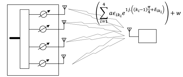
Figure 1: Illustration of measurement with all antennas turned ON

We illustrate the errors of $i^{\text{th}}$ antenna in Fig. 2. Here $\epsilon_{\text{ph},ik}$ denotes the nonideal scaling factor in phase shifter amplitude for $i^{\text{th}}$ antenna with $k^{\text{th}}$ phase, $\epsilon_{\text{ant},i}$ denotes the nonideal scaling factor in the combination of amplifier gain and antenna gain for antenna path $i$, and $\epsilon_{ik}=\left(\epsilon_{\text{ph},ik}\right)\left(\epsilon_{\text{ant},i}\right)$. The phase error in the phase shifter is noted as $\delta_{\text{ph},ik}$, while the phase error in the antenna path with respect to a nominal phase common to all antenna paths is denoted by $\delta_{\text{ant},i}$, and total phase error is noted as $\delta_{ik}=\delta_{\text{ph},ik}+\delta_{\text{ant},i}$.

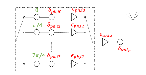
Figure 2: Illustration of errors for $i^{\text{th}}$ antenna.

For explicit calibration we would like to estimate $a\epsilon_{ik},\left(k-1\right)\pi/4+\delta{}_{ik}$ for all $i,k$. We also use a shorter notation $\phi_{ik}=\left(k-1\right)\pi/4+\delta{}_{ik}$, also its estimate is indicated with a hat as $\hat{\phi}_{ik}$ . We also define $b_{ik}=a\epsilon_{ik}$ and learn $b_{ik}$. Its estimate is indicated as $\hat{b}_{ik}$. We assume that we can make only power measurements and the measurements are made in the far-field boresight direction. Note that the absolute value of $\phi_{ik}$ cannot be measured using power measurements, since all power measurements remain invariant under a constant added to $\phi_{ik}$, i.e if the system had ${\phi_{ik}+c}$ for a constant c, all the power measurements would remain the same. Hence we set $\phi_{00}$ as a reference for measuring the phases. Hence the goal of our explicit calibration is to measure $b_{ik}$ for all $(i,k)$ and $\phi_{ik}-\phi_{00}$ for all ($i,k)\neq(0,0)$. We also use the notation Ant$i$Ph$k$ for $\phi_{ik}$ for easily recognizing the index for antenna and phase. The term $M_{ik}$ is the power measured with only $i^{\text{th}}$ antenna turned on at $k^{\text{th}}$ phase, and $M_{ik,mn}$ is the power measured with $i^{\text{th}}$ antenna turned on at $k^{\text{th}}$ phase together with $m^{\text{th}}$ antenna turned on at $n^{\text{th}}$ phase.

III Algorithm for measuring the antenna errors

Our algorithm for measuring the errors are as follows:

Step 1, Individual power measurements: The first step of our algorithm is to measure power with only single antenna turned ON, going through all antennas and all phases. We denote this power measurement by $M_{ik}$ where $i$ denotes the antenna index and $k$ denotes the phase index. Thus this takes $4\times 8=32$ measurements. With these measurements, $\hat{b}_{ik}=\sqrt{M_{ik}}$ can be obtained.

Remark 1.

Since we can make only power measurements, the phase errors cannot be measured from individual measurements. Using power measurements, only the difference between the phases at two antennas are obtained, for example with Ant0 and Ant1 ON with phase $\theta_{0}$ and rest of the antennas OFF, the received power is $M_{10,00}=b_{00}^{2}+b_{10}^{2}+2b_{10}b_{00}\cos(\phi_{10}-\phi_{00})$ in the absence of thermal noise. We estimate $\cos(\hat{\phi}_{10}-\hat{\phi}_{00})$ as follows (in presence of noise):

$$\cos(\hat{\phi}_{10}-\hat{\phi}_{00})=\left(4M_{10}M_{00}\right)^{-\frac{1}{2}}\cdot\left(M_{10,00}-M_{10}-M_{00}\right).$$ (2)

In general $\cos(\phi_{ik}-\phi_{mn})$ can be obtained from the measurements $M_{ik,mn},M_{ik},M_{mn}$ as

$$\cos(\hat{\phi}_{ik}-\hat{\phi}_{mn})=\left(4M_{ik}M_{mn}\right)^{-\frac{1}{2}}\cdot\left(M_{ik,mn}-M_{ik}-M_{mn}\right).$$ (3)

Step 2, Setting the reference: We choose $\phi_{00}$ as reference and we can estimate other $\phi_{ik}$ with respect to $\phi_{00}$, i.e., we can obtain $\hat{\phi}_{ik}-\hat{\phi}_{00}$. Henceforth we will use $\hat{\phi}_{00}=0$ in this report. To describe our algorithm for measuring the phase errors we use the illustration in Fig. 3 for antennas and phases.

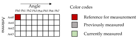
Figure 3: Illustration of antennas and phases.

The measurements give only angle differences in the form $\cos(\hat{\phi}_{10}-\hat{\phi}_{00})$, hence the phases cannot be obtained uniquely from a single measurement, since $\cos^{-1}\left(\right)$ is not unique in an interval of 2π, i.e. $\cos\left(x\right)=\cos(2\pi-x).$ Hence we need at least two measurements with respect to two reference phases for uniquely obtaining the phases. Fig. 4 illustrates the two references, the second reference is chosen as Ant1Ph$R_{1}$ where Ph$R_{1}$ is to be determined, $R_{1}$ could be any of $\left\{0,\ldots,7\right\}.$ The second reference could have been from any other antenna, but we choose Ant1. We will describe in next step how to choose Ph$R_{1}$ and how to estimate the phase of the second reference.

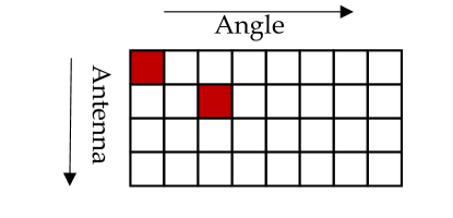
Figure 4: Two references for measuring the phases: Ant0Ph0 and Ant1Ph$R_{1}$

Step 3, Determining a second reference: The other phases $\phi_{ik},i>2$ are to be estimated with respect to both the references to uniquely obtain $\hat{\phi}_{ik}$ from $\cos(\hat{\phi}_{ik})$ and $\cos(\hat{\phi}_{ik}-\hat{\phi}_{1R_{1}})$. For uniquely solving $\hat{\phi}_{ik}$ from the values of $\cos(\hat{\phi}_{ik})$ and $\cos(\hat{\phi}_{ik}-\hat{\phi}_{1R_{1}})$, we need that $\hat{\phi}_{1R_{1}}\neq 0$. Also we need $\hat{\phi}_{1R_{1}}\neq\pi$, this is because $\cos(x)=\cos(-x)$ and $\cos(x-\pi)=\cos(-x-\pi)$ which prevents a phase $x$ from being resolved after obtaining $\cos()$ values with respect to 0 and π, because –x also gives same $\cos\left(\right)$ values with respect to 0 and π. We propose to choose Ph$R_{1}$ so that $\left\lvert\hat{\phi}_{1R_{1}}\right\lvert$ is close to π/2. We estimate all the phases of Ant1 with respect to Ant0Ph0 following 3 and choose Ph$R_{1}$ so that $\left\lvert\cos(\hat{\phi}_{1R_{1}}-\hat{\phi}_{00})\right\lvert=\left\lvert\cos(\hat{\phi}_{1R_{1}})\right\lvert$ is closest to zero. This is illustrated in Fig. 5 .

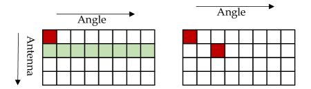
Figure 5: Figure 5: Choosing second reference.

To resolve the ambiguity of sign of $\hat{\phi}_{1R_{1}}$, we can check the value of $\cos()$ values on the phase that is ahead of $\hat{\phi}_{1R_{1}}$ by two indices. If $\hat{\phi}_{1R_{1}}$ was close to $-\pi/2$, then shifting the phase value forward twice from $R_{1}$ will cause the new phase to be close to zero, since the phase quantization in our case is with separation $\pi/4$. Thus $\hat{\phi}_{1(R_{1}+2)\text{mod}8}$ will be close to 0, i.e., $\cos\left(\hat{\phi}_{1(R_{1}+2)\text{mod}8}\right)$ will be close to +1. If $\hat{\phi}_{1R_{1}}$ was close to (+π)/2, then shifting the phase value forward twice from $R_{1}$ will cause the new phase to be close to π, i.e., $\hat{\phi}_{1(R_{1}+2)\text{mod}8}$ will be close to π, $\cos\left(\hat{\phi}_{1(R_{1}+2)\text{mod}8}\right)$ will be close to -1. This is illustrated in Fig. 6.

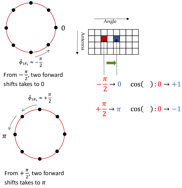
Figure 6: Resolving the sign of $\hat{\phi}_{1R_{1}}$ by looking at the value of $\cos\left(\hat{\phi}_{1(R_{1}+2)\text{mod}8}\right)$

Thus if $\cos\left(\hat{\phi}_{1(R_{1}+2)\text{mod}8}\right)$ is close to +1, then we choose $\hat{\phi}_{1R_{1}}$ close to $-\pi/2$. If $\cos\left(\hat{\phi}_{1(R_{1}+2)\text{mod}8}\right)$ is close to -1 then we choose $\hat{\phi}_{1R_{1}}$ close to $\pi/2$. This method for resolving the sign of $\hat{\phi}_{1R_{1}}$ can be used for the case with arbitrary number of quantization bits $Q$ for the number of phases, with $Q\geq 3$: we only need to look at whether $\cos\left(\hat{\phi}_{1(R_{1}+2^{Q-1})\text{mod}2^{Q}}\right)$ is closer to +1 or -1.

Step 4, Obtain all phases of Ant2, Ant3 with reference to Ant0Ph0, Ant1Ph$R_{1}$: Now the phases of the other antennas are estimated with respect to the references. For example for estimating $\phi_{20}$, Ant2 with Ph0 and Ant0 with Ph0 are turned ON with all other antennas turned OFF and the power is measured. Then Ant2 with Ph0 and Ant1 with Ph$R_{1}$ are turned ON with all other antennas turned OFF and power is measured. From the two power measurements $\cos(\hat{\phi}_{20})$and $\cos(\hat{\phi}_{20}-\hat{\phi}_{1R_{1}})$ are obtained. This step is illustrated in Fig. 8.

We now illustrate how to estimate $\phi_{ik}$ from the two values $A=\cos(\hat{\phi}_{ik}-\hat{\phi}_{00})$, $B=\cos(\hat{\phi}_{ik}-\hat{\phi}_{1R_{1}})$. We include $\hat{\phi}_{00}$ in the calculations, to show the steps with more generality, even though we had initially set $\hat{\phi}_{00}=0$.

$$A=\cos(\hat{\phi}_{ik}-\hat{\phi}_{00})=\cos\hat{\phi}_{ik}\cos\hat{\phi}_{00}+\sin\hat{\phi}_{ik}\sin\hat{\phi}_{00}$$ (4)

$$B=\cos(\hat{\phi}_{ik}-\hat{\phi}_{1R_{1}})=\cos\hat{\phi}_{ik}\cos\hat{\phi}_{1R_{1}}+\sin\hat{\phi}_{ik}\sin\hat{\phi}_{1R_{1}}$$ (5)

$$\left[\begin{array}[]{c}A\\ B\end{array}\right] =\left[\begin{array}[]{cc}\cos\hat{\phi}_{00}&\sin\hat{\phi}_{00}\\ \cos\hat{\phi}_{1R_{1}}&\sin\hat{\phi}_{1R_{1}}\end{array}\right]\left[\begin{array}[]{c}\cos\hat{\phi}_{ik}\\ \sin\hat{\phi}_{ik}\end{array}\right]$$ (12)

$$=K_{00,1R_{1}}\left[\begin{array}[]{c}\cos\hat{\phi}_{ik}\\ \sin\hat{\phi}_{ik}\end{array}\right]$$ (15)

Now $K_{00,1R_{1}}$ is invertible if $\sin(\hat{\phi}_{00}-\hat{\phi}_{1R_{1}})\neq 0$ i.e., if $\hat{\phi}_{1R_{1}}\neq\hat{\phi}_{00}+k\pi,k\in Z$. This is ensured by our choice of $\hat{\phi}_{1R_{1}}$. By solving the previous equation, we have

$$\left[\begin{array}[]{c}\cos\hat{\phi}_{ik}\\ \sin\hat{\phi}_{ik}\end{array}\right]=K_{00,1R_{1}}^{-1}\left[\begin{array}[]{c}A\\ B\end{array}\right]$$ (20)

Now we can obtain $\hat{\phi}_{ik}=\text{Angle}(e^{1j.\hat{\phi}_{ik}}))=\text{Angle}(\cos\left(\hat{\phi}_{ik}\right)+1j.\sin\left(\hat{\phi}_{ik}\right))$. When we have noisy measurements, we can say

$$\left[\begin{array}[]{c}u\\ v\end{array}\right]=K_{00,1R_{1}}^{-1}\left[\begin{array}[]{c}A\\ B\end{array}\right]$$ (21)

$$\hat{\phi}_{ik}=\text{Angle}(u+1j.v)$$ (22)

Step 5, Determine Ant2PhR2: For measuring all the phases for Ant0, we need two references. One of the references can be Ant1Ph$R_{1}$. We choose the other reference as Ant2Ph$R_{2}$. Similar to how Ant1Ph$R_{1}$ was chosen in relation to Ant0Ph0, requiring the two references to be approximately π/2 apart, we now choose Ant2Ph$R_{2}$ in relation to Ant1Ph$R_{1}$. Ph$R_{2}$ is chosen from the phases of Ant2 such that so that $\cos(\hat{\phi}_{2R_{2}}-\hat{\phi}_{1R_{1}})$ is closest to zero. We do this by looking at the estimated values of the phases of Ant2.

Step 6, Estimate all remaining phases of Ant0 with reference to Ant1Ph$R_{1}$, Ant2PhR2: Ant0Ph0 was set as zero for reference, the remaining phases of Ant0 is estimated with reference to Ant1Ph$R_{1}$ and Ant2Ph$R_{2}$. This is illustrated in Fig. 8 and is similar to Step 3.

Figure 7: Estimation of phases on Ant2 and Ant3

Figure 8: Estimation of phases on Ant0

Step 7, Determine Ant2Ph$R_{3}$: The remaining phases to be estimated are of Ant1. For this we need two references, one of them can be Ant0Ph0. The other reference can be from one of the remaining antennas. We choose the other reference as Ant2Ph$R_{3}$, it is chosen requiring the two references to be approximately π/2 apart, we make sure that $\left\lvert\cos(\hat{\phi}_{2R_{3}}-\hat{\phi}_{00})\right\lvert=\left\lvert\cos(\hat{\phi}_{2R_{3}})\right\lvert$ is closest to zero. We perform this by looking at the estimated values of the phases of Ant2.

Step 8, Estimate all remaining phases of Ant1 with reference to Ant0Ph$R_{0}$, Ant2Ph$R_{3}$: Now the remaining phases of Ant1 is estimated with reference to Ant0Ph0 and Ant2Ph$R_{3}$. This is illustrated in Fig. 9. Note that all the phases of Ant1 were already measured with respect to Ant0Ph0 while Ant1Ph$R_{1}$ was being chosen. Now the new measurements are required only with reference to Ant2Ph$R_{3}$.

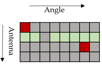
Figure 9: Phases of Ant1 is estimated with respect to Ant0Ph0 and Ant2Ph$R_{3}$

The individual power measurements for obtaining the gain errors are $4\times 8=32$. For obtaining the phase, all the phases of all the antennas require two measurements, except for Ant0Ph0 which needs no measurement and for Ant1Ph$R_{1}$ which takes only one measurement; this gives $2\times 4\times 8-2\times 2+1=61$. Total number of measurements is thus 93. For general N and Q the number of measurements can be similarly calculated as $3\times N\times 2^{Q}-3$

III-A Optimization

We perform a least squared optimization to minimize the error in the estimates due to noise in the measurements. Let $M_{ind}\left(l\right)$ indicate the $l^{\text{th}}$ individual power measurement, let $i_{l}$ be the antenna index and let $k_{l}$ be the phase index involved in $l^{\text{th}}$ measurement.

$$M_{ind}\left(l\right)=\left\lvert b_{i_{l}k_{l}}e^{1j.\left(\phi_{i_{l}k_{l}}\right)}+w_{l}\right\lvert^{2}.$$ (23)

Here $w_{l}$ is additive white Gaussian noise (AWGN). And let $M_{pair}(m)$ indicate the $m^{\text{th}}$ pairwise power measurement, $i_{m}^{(1)},i_{m}^{(2)}$ be the two antennas involved in $m^{\text{th}}$ pairwise power measurement. Similarly $k_{m}^{(1)},k_{m}^{(2)}$ are the phase indices.

$$M_{pair}(m)=\left\lvert b_{i_{m}^{(1)}k_{m}^{(1)}}e^{1j.\phi_{i_{m}^{(1)}k_{m}^{(1)}}}+b_{i_{m}^{(2)}k_{m}^{(2)}}e^{1j.\phi_{i_{m}^{(2)}k_{m}^{(2)}}}+w_{m}\right\lvert^{2}$$ (24)

Again $w_{m}$ is AWGN. We now change the variables to $a_{ik}e^{1j.\phi_{ik}}=a_{Rik}+1j.a_{Cik}$ and perform a least squares error optimization with respect to the power measurements.

$$\underset{}{\text{Minimize}}\sum_{l}\left(\left\lvert b_{Ri_{l}k_{l}}+1j.b_{Ci_{l}k_{l}}+w_{l}\right\lvert^{2}-M_{ind}(l)\right)$$

$$\hphantom{\underset{}{\text{Minimize}}}+\sum_{m}\Big{(}\left|b_{Ri_{m}^{(1)}k_{m}^{(1)}}+1j.b_{Ci_{m}^{(1)}k_{m}^{(1)}}+b_{Ri_{m}^{(2)}k_{m}^{(2)}}\right.$$

$$\hphantom{\underset{}{\text{Minimize}}+\sum_{m}\Big{(}}\left.+1j.b_{Ci_{m}^{(2)}k_{m}^{(2)}}+w_{m}\right|^{2}-M_{pair}(m)\Big{)}$$ (25)

The start point for the optimization is taken from the solution obtained from our previous calculation. If we choose the error-free phase and gain values as the starting point, we observed that the optimization does not converge to the correct solution in our simulations.

IV Simulation Results

We simulate our algorithms with $b_{ik}$ drawn uniformly from $[-1.5,+1.5]$ in dB. The signal to noise ratio (SNR) in our measurements is determined by the power of the noise $w$ in (23),(24) with signal power set at 0 dB. Phase error $\delta_{\text{ph},ik}$ is drawn uniformly from $[-10,+10]$ in degrees. Fixed phase errors $\delta_{\text{ant},i}$ on antennas are drawn randomly from $[-180,+180]$ in degrees. For the solution obtained from our algorithm without the least squared optimization, we use Err_max to denote the maximum error among all the phase estimates for a given array, and we have Err_avg as the average error. Similarly, after the least squared optimization, we have the terms Err_max_opt and Err_avg_opt. The error in calibration of the phase is given in Fig. 10 and the error in calibration of the amplitude gain is given in Fig. 11. The plots are obtained by averaging over 1000 iterations for each SNR. The average of the maximum error and average error for phases are calculated as $\mathbb{E}\left[\underset{i,k}{\text{max}}\left(\underset{l\in\mathbb{Z}}{\text{min}}\left\lvert\phi_{ik}-\hat{\phi}_{ik}+l2\pi\right\lvert\right)\right]$ and $\mathbb{E}\left[\underset{l\in\mathbb{Z}}{\text{min}}\left\lvert\phi_{ik}-\hat{\phi}_{ik}+l2\pi\right\lvert\right]$ respectively where the expectation is over the iterations and $(i,k)\neq(0,0)$. Similarly the average of maximum error for gain is calculated in dB as $\mathbb{E}\left[\underset{i,k}{\text{max}}\left(20\log 10\left\lvert\left\lvert b_{ik}-\hat{b}_{ik}\right\lvert/b_{ik}+1\right\lvert\right)\right]$, and the average error for gain is calculated as $\mathbb{E}\left[20\log 10\left\lvert\left\lvert b_{ik}-\hat{b}_{ik}\right\lvert/b_{ik}+1\right\lvert\right]$where the expectation is over the iterations and all $i,k$.

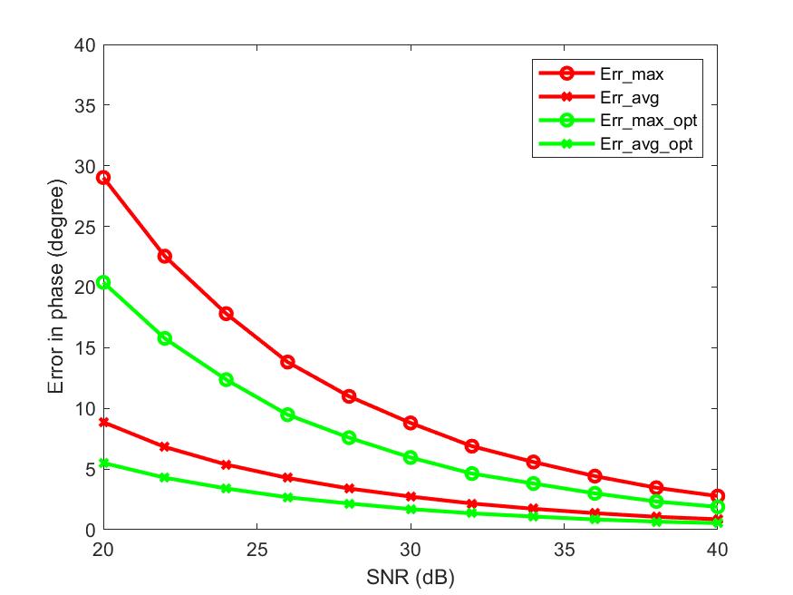
Figure 10: Comparison of error in phase calibration

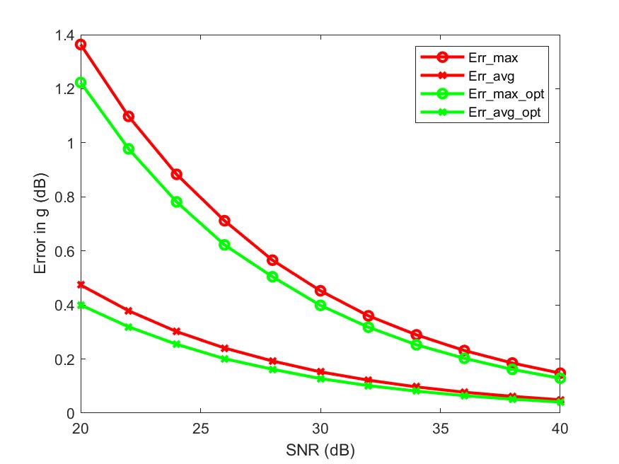
Figure 11: Comparison of percentage error in gain calibration.

We simulate the REV method with $\delta_{\text{ant},i}$ drawn in the same way as in the previous simulation. However, there are no phase dependent errors $\delta_{\text{ph},ik}$ this case. Also, we have $b_{i}$ dependent only on the antenna, instead of $b_{ik}$ dependent on both antenna and phase. For the solution from the REV method, we denote the maximum error among the three $\delta_{\text{ant},i}$ as Err_max_REV and the average error over the three phases as Err_avg_REV. For rotating the phase of each antenna in the REV methods, we go through eight phases. Hence with two iterations of REV method and four antennas, the total number of measurements is $2\times 4\times 8=64$. We compare the performance of REV method with our algorithm with the least squared optimization. Our original algorithm is designed for the case with phase dependent errors. Hence for the case with no phase-dependent errors, we average the errors across the phases. For our solution, we denote the maximum error among the three $\delta_{\text{ant},i}$ as Err_max_opt and the average error over the three phases as Err_avg_opt. The error in calibration of the phase is given in Fig. 12 and the error in calibration of the amplitude gain is given in Fig. 13. We note that our method performs better than the REV method.

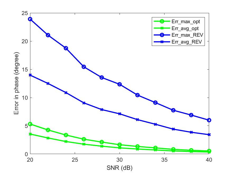
Figure 12: Comparison with REV method for error in phase calibration

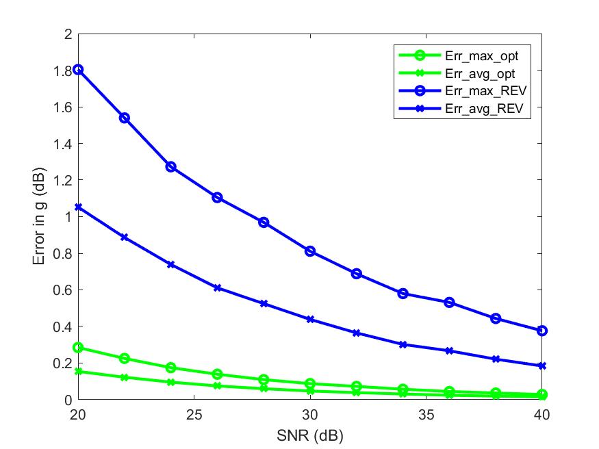
Figure 13: Comparison with REV method for percentage error in gain calibration.

We also demonstrate the usefulness of our method to improve the coverage. We consider an ideal codebook designed for an omnidirectional linear 4-antenna array with separation between antennas as $\lambda/2$, with $\lambda$ denoting the wavelength of the radio wave from the antenna. This is illustrated in Fig. 14. Due to symmetry we can describe the antenna pattern using single angle parameter $\Theta$. The path difference of $\left(\lambda/2\right)\sin\left(\Theta\right)$ corresponds to a phase difference of $\pi\sin\left(\Theta\right)$. Similarly considering all the rays from four antennas, and a code with phases $[\phi_{0i_{0}},\phi_{1i_{1}},\phi_{2i_{2}},\phi_{3i_{3}}]$ on the antennas, the power in the direction $\Theta$ is

$$P(\Theta)= \left|1+e^{1j.\left(\phi_{1i_{1}}+\pi\sin\left(\Theta\right)\right)}\right.$$

$$\left.+e^{1j.\left(\phi_{2i_{2}}+2\pi\sin\left(\Theta\right)\right)}+e^{1j.\left(\phi_{3i_{3}}+3\pi\sin\left(\Theta\right)\right)}\right|^{2}.$$ (26)

Figure 14: Antenna illustration.

For a quantized codebook with multiples of $\pi/4$ as the permitted phases in the absence of errors, we design codes for directions $[90,19,40,-19,-40,0]$ in degree. For each direction we choose the codeword that gives maximum power according to (26).

Let $\hat{\phi}_{ik}$ be the estimated phases in presence of errors at the antennas obtained by our algorithm. For a given code which gives phases $[\hat{\phi}_{0i_{0}},\hat{\phi}_{1i_{1}},\hat{\phi}_{2i_{2}},\hat{\phi}_{3i_{3}}]$ on the antennas and corresponding magnitudes $[\hat{b}_{0i_{0}},\hat{b}_{1i_{1}},\hat{b}_{2i_{2}},\hat{b}_{3i_{3}}]$, the power in a direction Θ is calculated as

$$\hat{P}(\Theta)$$

$$=\left|\hat{b}_{0i_{0}}e^{1j.\hat{\phi}_{0i_{0}}}+\hat{b}_{1i_{1}}e^{1j.\left(\hat{\phi}_{1i_{1}}+\pi\sin\left(\Theta\right)\right)}\right.$$

$$\quad\left.+\hat{b}_{2i_{2}}e^{1j.\left(\hat{\phi}_{2i_{2}}+2\pi\sin\left(\Theta\right)\right)}+\hat{b}_{3i_{3}}e^{1j.\left(\hat{\phi}_{2i_{2}}+3\pi\sin\left(\Theta\right)\right)}\right|^{2}.$$ (27)

Subsequently for each code direction, we can choose the code that gives the maximum power $\hat{P}(\Theta)$ according to our calculation. For the codeword designed for error-free scenario and for the codeword designed with estimated errors, we then calculate the observed EIRP. We obtain the CDF (averaged over multiple error instances) of scaled EIRP in a sphere around the phased array. The CDF is illustrated in Fig. 15. We consider two cases SNR of 20 dB and SNR of 30 dB in measurements for our calibration algorithm. The variables $b_{ik},\delta_{\text{ph},ik},\delta_{\text{ant},ik}$ are generated as described at the beginning of this section. The EIRP scaling is with respect to the maximum possible EIRP in the simulation setup .i.e. when the $b_{ik}$’s are $1.5$ dB and combine coherently. We observe that our calibration significantly improves the coverage. In terms of 3GPP requirements, on the average, with 20 dB SNR we can observe about 1.5 dB improvement in 50%-tile EIRP and 0.73 dB improvement in 99%-tile EIRP compared to the case without calibration.

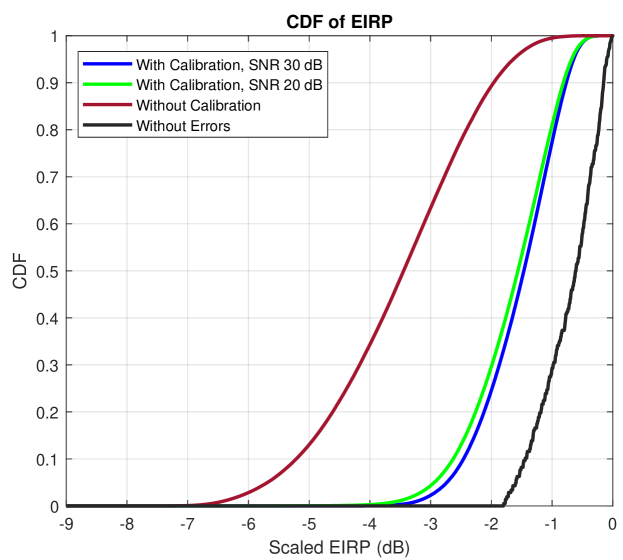
Figure 15: Comparison of CDF performance.

V Conclusions

We proposed a method for explicit calibration of phased arrays using only power measurements. We find the gain errors and phase errors using $3\times N\times 2^{Q}-3$ measurements where $N$ is the number of antennas and $Q$ is the number of quantization bits for phased array. Our method consists of an algorithm to solve for the values of the errors by simple step by step calculation for the phase values compared to chosen reference values. Subsequently we apply a least squared optimization around the initial solution, to reduce the estimation error. Our method uses relatively low number of measurements, demonstrates more accurate results compared to the REV method, and provides improvement in coverage.

References

- [1] S. Mano and T. Katagi, “A method for measuring amplitude and phase of each radiating element of a phased array antenna,” Electronics and Communications in Japan (Part I: Communications), vol. 65, no. 5, pp. 58–64, 1982.
- [2] N. Kojima, K. Shiramatsu, I. Chiba, T. Ebisui, and N. Kurihara, “Measurement and evaluation techniques for an airborne active phased array antenna,” in Proceedings of International Symposium on Phased Array Systems and Technology, Oct 1996, pp. 231–236.
- [3] T. Takahashi, Y. Konishi, S. Makino, H. Ohmine, and H. Nakaguro, “Fast measurement technique for phased array calibration,” IEEE Transactions on Antennas and Propagation, vol. 56, no. 7, pp. 1888–1899, 2008.
- [4] K.-M. Lee, R.-S. Chu, and S.-C. Liu, “A built-in performance-monitoring/fault isolation and correction (pm/fic) system for active phased-array antennas,” IEEE transactions on antennas and propagation, vol. 41, no. 11, pp. 1530–1540, 1993.
- [5] G. A. Hampson and A. B. Smolders, “A fast and accurate scheme for calibration of active phased-array antennas,” in Antennas and Propagation Society International Symposium, 1999. IEEE, vol. 2. IEEE, 1999, pp. 1040–1043.