Convergence rates for shallow neural networks learned by gradient descent

Abstract

In this paper we analyze the $L_{2}$ error of neural network regression estimates with one hidden layer. Under the assumption that the Fourier transform of the regression function decays suitably fast, we show that an estimate, where all initial weights are chosen according to proper uniform distributions and where the weights are learned by gradient descent, achieves a rate of convergence of $1/\sqrt{n}$ (up to a logarithmic factor). Our statistical analysis implies that the key aspect behind this result is the proper choice of the initial inner weights and the adjustment of the outer weights via gradient descent. This indicates that we can also simply use linear least squares to choose the outer weights. We prove a corresponding theoretical result and compare our new linear least squares neural network estimate with standard neural network estimates via simulated data. Our simulations show that our theoretical considerations lead to an estimate with an improved performance in many cases.

, , and

1 Introduction

1.1 Scope of this article

Understanding the success of neural networks in practical applications (see, e.g., Krizhevsky, Sutskever, and Hinton (2012), Kim (2014), Wu et al. (2016) or Silver et al. (2017)) is arguably one of the most important goals of machine learning theory today. The problem has been studied in a statistical context, by analyzing empirical risk minimizers based on various classes of neural networks and under different assumptions on the target function (see, e.g., Schmidt-Hieber (2020), Kohler, Krzyżak and Langer (2019), Suzuki and Nitanda (2019) and the literature cited therein). A complementary line of work (see, e.g., Choromanska et al. (2015), Allen-Zhu and Li (2019), Ghorbani et al. (2019) and the literature cited therein) deals with the optimization procedure of the networks and analyzes the gradient descent routine and its variants. Although both areas partially contribute to the theoretical understanding of deep learning, they each omit important parts in their analysis. In particular, they either work in an ideal setting without any optimization error or analyze an optimization procedure without any statistical setting. With the goal in mind to bridge the gap between these two research areas, the aim of this work is to answer the following question:

Can we derive rate of convergence results for neural network estimators learned by gradient descent in a nonparametric regression setting?

For simplicity, we restrict ourselves to the class of shallow neural networks, i.e., neural networks with only one hidden layer and assume regression functions with suitable decaying Fourier transforms (see (12)).

1.2 Nonparametric regression

We consider a $\mathbb{R}^{d}\times\mathbb{R}$–valued random vector $(X,Y)$, where $X$ is the so–called observation vector and $Y$ is the so-called response. Assume the condition ${\mathbf{E}}\{Y^{2}\}<\infty$. We are interested in the functional correlation between the response $Y$ and the observation vector $X$. Particulary, we are searching for a function $f^{*}:\mathbb{R}^{d}\to\mathbb{R}$ such that

$${\mathbf{E}}\left\{|f^{*}(X)-Y|^{2}\right\}=\min_{f:\mathbb{R}^{d}\to\mathbb{R}}{\mathbf{E}}\left\{|f(X)-Y|^{2}\right\}.$$

This minimum holds for $f^{*}(x)=m(x)={\mathbf{E}}\{Y|X=x\}$ (see Section 1.1 in Györfi et al. (2002)), which is why $m$ is the so-called regression function. But, in applications the distribution of $(X,Y)$ is unknown. A basic problem in statistics is to recover the unknown regression function $m$ from a sample of $(X,Y)$, i.e., a data set

$${\mathcal{D}}_{n}=\left\{(X_{1},Y_{1}),\ldots,(X_{n},Y_{n})\right\},$$ (1)

where $(X,Y)$, $(X_{1},Y_{1})$, …, $(X_{n},Y_{n})$ are independent and identically distributed (i.i.d.). Particulary, we are searching for an estimator

$$m_{n}(\cdot)=m_{n}(\cdot,{\mathcal{D}}_{n}):\mathbb{R}^{d}\rightarrow\mathbb{R}$$

of $m$ such that the so–called $L_{2}$ error

$$\int|m_{n}(x)-m(x)|^{2}{{\mathbf{P}}}_{X}(dx)$$

is “small” (cf., e.g., Györfi et al. (2002) for a systematic introduction to nonparametric regression and a motivation for the $L_{2}$ error).

1.3 Least squares neural network estimators

Neural networks try to mimic the human brain in order to define classes of functions. The starting point is a very simple model of a nerve cell, in which some kind of thresholding is applied to a linear combination of the outputs of other nerve cells. This leads to functions of the form

$$f(x)=\sigma\left(\sum_{j=1}^{d}w_{j}\cdot x^{(j)}+w_{0}\right)\quad(x=(x^{(1)},\dots,x^{(d)})^{T}\in\mathbb{R}^{d}),$$

where we call $w_{0}$, …, $w_{d}\in\mathbb{R}$ the weights of the neuron and $\sigma:\mathbb{R}\rightarrow\mathbb{R}$ the activation function. Traditionally, so–called squashing functions are chosen as activation functions, which are nondecreasing and satisfy $\lim_{x\rightarrow-\infty}\sigma(x)=0$ and $\lim_{x\rightarrow\infty}\sigma(x)=1$. An example is the so-called sigmoidal or logistic squasher

$$\sigma(x)=\frac{1}{1+\exp(-x)}\quad(x\in\mathbb{R}).$$ (2)

Recently, also unbounded activation functions are used, e.g., the ReLU activation function

$$\sigma(x)=\max\{x,0\}.$$

Some works like Sonoda, Ishikawa and Ikeda (2021), Sitzmann et al. (2020) and the literature cited therein, consider periodic activation functions of the form $\sigma(t)=\sigma(t+T)$, where $T$ denotes the length of the period.

The most simple form of neural networks are shallow networks, i.e., neural networks with one hidden layer, in which a simple linear combination of the above neurons is used to define a function $f:\mathbb{R}^{d}\rightarrow\mathbb{R}$ by

$$f(x)=\sum_{k=1}^{K}\alpha_{k}\cdot\sigma\left(\sum_{j=1}^{d}\beta_{k,j}\cdot x^{(j)}+\beta_{k,0}\right)+\alpha_{0}.$$ (3)

Here $K\in\mathbb{N}$ is the number of neurons. The weights $\alpha_{k}\in\mathbb{R}$ $(k\in\{0,\dots,K\})$, $\beta_{k,j}\in\mathbb{R}$ $(k\in\{1,\dots,K\},j\in\{0,\dots,d\})$ are then fitted to the data (1) in order to define an estimate of the regression function. This can be achieved for example by applying the principle of least squares, i.e., by defining the regression estimator $m_{n}$ by

$$m_{n}(\cdot)=\operatorname*{arg\,min}_{f\in{\mathcal{F}}}\frac{1}{n}\sum_{i=1}^{n}|Y_{i}-f(X_{i})|^{2},$$ (4)

where ${\mathcal{F}}$ is the set of all functions of the form (3) with a fixed number of neurons $K$ and fixed activation function $\sigma$.

The rate of convergence of shallow neural network regression estimates has been analyzed in Barron (1994) and McCaffrey and Gallant (1994). Barron (1994) proved a dimensionless rate of $n^{-1/2}$ (up to some logarithmic factor), provided the Fourier transform of the regression function has a finite first moment, which basically requires that the function becomes smoother with increasing dimension $d$ of $X$. McCaffrey and Gallant (1994) showed for any $\epsilon>0$ a rate of $n^{-\frac{2p}{2p+d+5}+\varepsilon}$ in case of a $p$-times continuously differentiable regression function, but their study was restricted to the use of a certain cosine squasher as activation function. As to related work, we mention Kůrková und Sanguinetti (2008) with further references.

In deep learning, neural networks with several hidden layers are used to define classes of functions. Here, the neurons are arranged in $\mathcal{L}\in\mathbb{N}$ layers, where the $k_{s}\in\mathbb{N}$ neurons in layer $s\in\{2,\dots,\mathcal{L}\}$ get the output of the $k_{s-1}$ neurons in layer $s-1$ as input, and where the neurons in the first layer are applied to the $d$ components of the input. We denote the weight between neuron $j$ in layer $s-1$ and neuron $i$ in layer $s$ by $w_{i,j}^{(s)}$. This leads to the following recursive definition of a neural network with $\mathcal{L}$ layers and $k_{s}$ neurons in layer $s\in\{1,\dots,\mathcal{L}\}$:

$$f(x)=\sum_{i=1}^{k_{\mathcal{L}}}w_{1,i}^{(\mathcal{L})}f_{i}^{(\mathcal{L})}(x)+w_{1,0}^{(\mathcal{L})}$$ (5)

for some $w_{1,0}^{(\mathcal{L})},\ldots,w_{1,k_{L}}^{(\mathcal{L})}\in\mathbb{R}$ and for $f_{i}^{(\mathcal{L})}$’s recursively defined by

$$f_{i}^{(s)}(x)=\sigma\left(\sum_{j=1}^{k_{s-1}}w_{i,j}^{(s-1)}f_{j}^{(s-1)}(x)+w_{i,0}^{(s-1)}\right)$$ (6)

for some $w_{i,0}^{(s-1)},\dots,w_{i,k_{s-1}}^{(s-1)}\in\mathbb{R}$, $s\in\{2,\dots,\mathcal{L}\}$, and

$$f_{i}^{(1)}(x)=\sigma\left(\sum_{j=1}^{d}w_{i,j}^{(0)}x^{(j)}+w_{i,0}^{(0)}\right)$$ (7)

for some $w_{i,0}^{(0)},\dots,w_{i,d}^{(0)}\in\mathbb{R}$.

The rate of convergence of least squares estimates based on multilayer neural networks has been analyzed in Kohler and Krzyżak (2017), Imaizumi and Fukumizu (2018), Bauer and Kohler (2019), Kohler, Krzyżak and Langer (2019), Suzuki and Nitanda (2019), Schmidt-Hieber (2020) and Kohler and Langer (2021). One of the main results obtained in this context shows that neural networks can achieve some kind of dimension reduction, provided the regression function is a composition of (sums of) functions, where the input dimension of each of the functions is at most $d^{*}<d$ (see Kohler and Langer (2020) for a motivation of such a function class). In Kohler and Krzyżak (2017) it was shown that in this case suitably defined least squares estimates based on multilayer neural networks achieve the rate of convergence $n^{-2p/(2p+d^{*})}$ (up to some logarithmic factor) for $p\leq 1$. This result also holds for $p>1$ provided the squashing function is suitably smooth as was shown in Bauer and Kohler (2019). Schmidt-Hieber (2020) showed the surprising result that this is also true for neural networks which use the non-smooth ReLU activation function. In Kohler and Langer (2021) it was shown that such results also hold for very simply constructed fully connected feedforward neural networks. Kohler, Krzyżak and Langer (2019) considered regression functions with low local dimensionality and demonstrated that neural networks are also able to circumvent the curse of dimensionality in this context. Results regarding the estimation of regression functions which are piecewise polynomials having partitions with rather general smooth boundaries by neural networks have been derived in Imaizumi and Fukumizu (2018). That neural networks can also achieve a dimension reduction in Besov spaces was shown in Suzuki and Nitanda (2019).

1.4 Gradient descent

In Subsection 1.3 the neural network regression estimates are defined as nonlinear least squares estimates, i.e., as functions which minimize the empirical $L_{2}$ risk over nonlinear classes of neural networks. In practice, it is usually not possible to find this global minimum and one tries to find a local minimum using, for instance, the gradient descent algorithm.

Denote by $f_{net,\mathbf{w}}$ the neural network defined by (5)–(7) with weight vector

$$\mathbf{w}=(w_{j,k}^{(s)})_{s=0,\dots,\mathcal{L},j=1,\dots,k_{s+1},k=0,\dots,k_{s}}$$

(where we set $k_{0}=d$ and $k_{\mathcal{L}+1}=1$), and set

$$F(\mathbf{w})=\frac{1}{n}\sum_{i=1}^{n}|Y_{i}-f_{net,\mathbf{w}}(X_{i})|^{2}.$$ (8)

Now gradient descent is used to minimize (8) with respect to $\mathbf{w}$. Here, set

$$\mathbf{w}(0)=\mathbf{v}$$ (9)

for some (usually randomly chosen) initial weight vector $\mathbf{v}$ and define

$$\mathbf{w}(t+1)=\mathbf{w}(t)-\lambda_{n}\cdot\nabla_{\mathbf{w}}F(\mathbf{w}(t))$$ (10)

for $t\in\{0,1,\dots,t_{n}-1\}$, where $\lambda_{n}>0$ is the stepsize and $t_{n}\in\mathbb{N}$ is the number of performed gradient descent steps. The estimate is then defined by

$${m}_{n}(\cdot)=f_{net,\mathbf{w}(t_{n})}(\cdot).$$ (11)

1.5 Main results

The main results in this article are threefold: Firstly, we analyze the rate of convergence of a shallow neural network regression estimate, where the weights are learned by gradient descent. Here we assume that the Fourier transform

$$\hat{F}:\mathbb{R}^{d}\rightarrow\mathbb{C},\quad\hat{F}(\omega)=\frac{1}{(2\pi)^{d/2}}\cdot\int_{\mathbb{R}^{d}}\exp(-i\cdot\omega^{T}x)\cdot m(x)\,dx$$

of the regression function $m(x)={\mathbf{E}}\{Y|X=x\}$ satisfies

$$|\hat{F}(\omega)|\leq\frac{c_{1}}{\|\omega\|^{d+1}\cdot(\log\|\omega\|)^{2}}\quad\mbox{for all }\omega\in\mathbb{R}^{d}\mbox{ with }\|\omega\|\geq 2$$ (12)

for some $c_{1}\in\mathbb{R}_{+}$. We show that if we use the logistic squasher as the activation function, if we choose the initial weights of the neural network randomly from some proper uniform distributions, and if we perform (up to some logarithmic factor) $n^{1.75}$ gradient descent steps with step size of order $1/n^{1.25}$ (up to some logarithmic factor) applied to some properly regularized empirical $L_{2}$ risk, then a truncated version of the estimate achieves (up to some logarithmic factor) the rate of convergence $1/\sqrt{n}$. This shows that the classical result from Barron (1994) also holds for a neural network estimate learned by gradient descent. Surprisingly, in this result a single random initialization of the weights is sufficient. Furthermore our proof clarifies that this result mainly holds because of the proper initialization of the weights and because of the good adjustment of the outer weights of the neural network during gradient descent. We also establish a minimax lower bound for the rate of convergence. It reveals that for large $d$ the obtained rate of convergence is in its exponent $-1/2$ close to the optimal minimax rate of convergence.
Secondly, we use our theoretical findings to simplify our estimate. Due to the fact that the optimization of the inner weights by gradient descent is not necessary in our result, it is evident that it should suffice to minimize the outer weights of the neural network. But this is (for fixed inner weights), in fact, a linear least squares problem, for which the optimal weights can easily be computed by solving a linear equation system. We define a corresponding linear least squares estimator with randomly selected inner weights, and show that for this estimator the same rate of convergence result holds as for our neural network estimator based on gradient descent. The big advantage of this estimator is that it can be computed much faster in applications.
Thirdly, we compare our (theoretically motivated) estimator to classical shallow neural networks learned by gradient descent on simulated data. In many cases we see a clear outperformance of our estimator over the classical ones.

1.6 Discussion of related results

Our result shows that it is possible to extend the classical result from Barron (1994) to the case of a neural network estimator learned by gradient descent. In contrast to Barron (1994), in which it was assumed that the Fourier transform $\hat{F}$ of the regression function has a finite first moment, i.e.,

$$\int_{\mathbb{R}^{d}}\|\omega\|\cdot|\hat{F}(\omega)|\,d\omega<\infty,$$ (13)

we need the slightly stronger assumption (12).

1.6.1 On related proof strategies

Stone (1982) showed that the optimal minimax rate of convergence for estimation of a $p$–times continuously differentiable regression function is $n^{-2p/(2p+d)}$. For fixed $p$ and increasing dimension $d$ this optimal rate gets worse in high dimensions (so–called curse of dimensionality). The rate $1/\sqrt{n}$ derived by Barron (1994) and also in this paper is independent of the dimension and does consequently not suffer from the curse of dimensionality. This is due to the fact that the existence of a first moment of the Fourier transform of the regression function basically requires that the smoothness of the regression function increases in case of a growing dimension (cf., Remarks 3 and 5 below).
For his statistical investigation, Barron (1994) used a result of Barron (1993) on the rate of approximation of a function with finite first moment of its Fourier transform by a shallow neural network. Barron (1993) obtained his deterministic approximation result by a probabilistic argument of Maurey (see Pisier (1980)). This approach was analyzed and modified by Igelnik and Fao (1995) and motivated them to propagate shallow neural networks with random $d$-dimensional weight vectors $\beta_{j}$ and biases $\gamma_{j}$ ($j\in\{1,\dots,K_{n}\}$). Here the non-linear optimization problem in Barron (1994) is reduced to a quadratic optimization problem on the outer weights $\alpha_{k}$ ($k\in\{1,\dots,K_{n}\}$). As an approximation result, the authors established rate of convergence of the mean squared error for Lipschitz continuous functions (see also Huang et al. (2006)).
Section 3 of the present paper deals with the investigation of statistical learning of such a neural network, combining methods of empirical process theory and stochastic type approximation, modifying and partially weakening Barron’s (1994) first moment condition. Beside the estimation and approximation error an optimization error is taken into account, i.e., networks trained by gradient descent are considered. In a rather general framework Rahimi and Recht (2006) obtained results on learning random neural networks guaranteeing assertion validity with high probability.
Under sharpened Barron conditions (higher moment conditions), which is satisfied, among other things, by solution functions of Kolmogorov PDEs, Goron (2021) established approximation, estimation and optimization error bounds for shallow neural network estimators with ReLU activation function and randomly generated internal weights and biases (see also Goron et al. (2020) with further literature).
In a more practically oriented result, Dudek (2019) proposed a method for shallow neural network regression estimates on how to choose the range of random inner weights and biases depending on the input data and the shape of the activation functions. The main result of our paper concerns a well-defined size of the range of the inner weights and biases, while in the proof, particulary in application of Lemma 5.1, the special shape of the logistic squasher is taken into account. It should be mentioned that for multilayer neural networks with randomly chosen inner weights and biases, Widrow et al. (2013) presented a gradient descent method for determing the outer weights.

1.6.2 On the optimization error of neural networks

There exist quite a few papers which try to show that neural network estimators learned by gradient descent have nice theoretical properties. The most popular approach in this context is the so–called landscape approach. Choromanska et al. (2015) used random matrix theory to derive a heuristic argument showing that the risk of most of the local minima of the empirical $L_{2}$ risk is not much larger than the risk of the global minimum. For networks with linear or quadratic activation function this claim could be validated, see, e.g. , Arora et al. (2018), Kawaguchi (2016), and Du and Lee (2018). However, these networks do not have good approximation properties. Consequently, it is not possible to derive comparable convergence rates from these results as in our work. Du et al. (2018) analyzed gradient descent applied to shallow neural networks in case of a Gaussian input distribution. But they used the expected gradient instead of the true gradient in their gradient descent routine and therefore their result cannot be applied to derive the same convergence rates as in our work. Liang et al. (2018) applied gradient descent to a modified loss function in classification, where it is assumed that the data can be interpolated by a neural network. Here, the second assumption is not satisfied in nonparametric regression and it is unclear whether the main idea (of simplifying the estimation by a modification of the loss function) can also be used in a regression setting. Brutzkus et al. (2018) prove that two-layer networks with ReLU activation function can learn linearly-separable data using stochastic gradient descent. Andoni et al. (2014) also consider two-layer networks and analyze the sample complexity of these networks for learning multidimensional polynomial functions of finite degree. But this result is based on exponential activation functions. For an overview of the literature concerning neural networks learned by gradient descent we also refer to Poggio, Banburski and Liao (2020).
Our result can be understood as a confirmation of the conjecture in the landscape approach in case of shallow neural networks. We show that with our random initialization of the inner weights of the neural network, with high probability they are chosen such that there exist values for the outer weights such that the corresponding neural network has a small empirical $L_{2}$ risk. So, if we define the local minima of the empirical $L_{2}$ risk as the minima which we get if we just choose the outer weights optimally and keep the values of the inner weights, then indeed most of the local minima of the empirical $L_{2}$ risk have a small value. This is related to the assertion of Goodfellow, Bengio and Courville (2015, pp. 3-5), who mention that machine learning algorithms heavily depend on the representation of the data. In particular, they consider the ability of deep learning to learn a good hierarchical representation of the data as a key aspect of its success. In our result the inner representation of the data used by our network depends on the randomly chosen inner weights, which are applied to the activation function. Hence, in our result the key feature of the neural networks is representation guessing instead of representation learning.
For a related topic, i.e., estimation of regression functions by generalizations of two layer radial basis function networks, the asymptotic behaviour of the gradient descent was analyzed in Javanmard, Mondelli and Montanari (2021) by using a so–called Wasserstein gradient descent approach. It remains unclear whether the approach can be extended to classical neural networks. In particular, it is unclear whether the results about shallow networks as in our article can be derived by this approach.

1.6.3 On results of overparametrized neural networks

Recently it was shown in quite a few papers that in case of suitably overparameterized neural networks gradient descent can find the global minimum of the empirical $L_{2}$ risk, cf., e.g., Kawaguchi and Huang (2019), Allen-Zhu, Li and Song (2019), Allen-Zhu, Li and Liang (2019), Arora et al. (2019a, 2019b), Du et al. (2018), Li and Liang (2018) and Zou et al. (2018). However, Kohler and Krzyżak (2019) presented a counterexample demonstrating that overparameterized neural networks, which basically interpolate the training data, in general do not generalize well. In this counterexample the regression function is constant zero and hence satisfies the assumption on the regression function imposed in our paper. In particular, this shows that results similar to the ones in our paper cannot be concluded from the papers cited above. We would also like to stress that our estimator does not use an overparameterization, because the numbers of weights of our neural networks in the theorems below are much smaller than the sample size.
Another approach to analyze overparameterized neural networks is the the so–called kernel approach (cf. Jacot, Gabriel and Hongler (2020) and the literature cited in Woodworth et al. (2020)). Here, neural networks are approximately described by kernel methods and a gradient descent in continuous time modelled by a differential equation leads to the so–called neural tangent kernel, which depends on the time. The asymptotic behaviour of this neural tangent kernel has been analyzed in Jacot, Gabriel and Hongler (2020), which leads to an asymptotic approximation of neural networks. Unfortunately this asymptotic approximation does not imply how the finite neural networks behave during learning.

1.6.4 On the generalization error of neural networks

The generalization of neural networks can also be analyzed within the classical Vapnik Chervonenkis theory (cf., e.g., Chapters 9 and 17 in in Györfi et al. (2002)). Here, the complexity of the underlying function spaces is measured by covering numbers, which can be bounded using the so–called Vapnik-Chervonenkis dimension (cf., e.g., Bartlett et al. (2019)). However, the resulting upper bounds on the generalization error might be too rough as during gradient descent the neural network estimator does not necessarly attend all functions from the underlying function space. One might sharpens the bound by using the so–called Rademacher complexity (cf., Koltchinski (2004)). For networks with quadratic activation function this has already been successfully done in Du and Le (2018), but unfortunately such neural networks do not have good approximation properties and similar results as in our work can therefore certainly not be derived. Also, we would like to stress that in our result we indeed analyze the generalization of neural networks within the classical Vapnik Chervonenkis theory.

1.7 Notation

Throughout the paper, the following notation is used: The sets of natural numbers, natural numbers including $0$, real numbers, nonegative real numbers and complex numbers are denoted by $\mathbb{N}$, $\mathbb{N}_{0}$, $\mathbb{R}$, $\mathbb{R}_{+}$ and $\mathbb{C}$, respectively. For $z\in\mathbb{R}$, we denote the smallest integer greater than or equal to $z$ by $\lceil z\rceil$ and the largest integer smaller or equal to $z$ by $\lfloor z\rfloor$. Let $D\subseteq\mathbb{R}^{d}$ and let $f:\mathbb{R}^{d}\rightarrow\mathbb{R}$ be a real-valued function defined on $\mathbb{R}^{d}$. We write $x=\arg\min_{z\in D}f(z)$ if $\min_{z\in{\mathcal{D}}}f(z)$ exists and if $x$ satisfies $x\in D$ and $f(x)=\min_{z\in{\mathcal{D}}}f(z)$. The Euclidean norm of $x\in\mathbb{R}^{d}$ is denoted by $\|x\|$. For $f:\mathbb{R}^{d}\rightarrow\mathbb{R}$

$$\|f\|_{\infty}=\sup_{x\in\mathbb{R}^{d}}|f(x)|$$

is its supremum norm. $S_{r}$ denotes the ball with radius $r$ in $\mathbb{R}^{d}$ and center $0$ (with respect to the Euclidean norm). We define the truncation operator $T_{\kappa}$ with level $\kappa>0$ as

$$T_{\kappa}u=\begin{cases}u\quad&\text{if}\quad|u|\leq\kappa\\ \kappa\cdot{\rm sign}(u)\quad&\text{otherwise}.\end{cases}$$

Constants are designated and numbered $c_{1},c_{2},\dots$. Each constant is assumed to be non-negative and, unless otherwise stated, absolute.

1.8 Outline

In Section 2 we present our main result concerning the rate of convergence of a shallow neural network estimator learned by gradient descent. In Section 3 we show that the same rate of convergence can also be achieved by a linear least squares estimator with much simpler computation. In Section 4 we compare the finite sample size behaviour of our linear least squares estimate via simulated data. Section 5 contains the proof of a key auxiliary result concerning the approximation error of shallow neural networks with randomly chosen inner weights, and the outline of the proofs of Theorem 2.1 and Theorem 3.1. The complete proofs of our main results are given in the supplement.

2 A neural network estimate learned by gradient descent

In this sequel we analyze shallow neural networks with $K_{n}$ hidden neurons and a constant term. As activation function we choose the logistic squasher (2). The networks are defined by

$$f_{net,\mathbf{w}}(x)=w_{1,0}^{(1)}+\sum_{j=1}^{K_{n}}w_{1,j}^{(1)}\cdot\sigma\left(\sum_{k=1}^{d}w_{j,k}^{(0)}\cdot x^{(k)}+w_{j,0}^{(0)}\right)=\alpha_{0}+\sum_{j=1}^{K_{n}}\alpha_{j}\cdot\sigma\left(\beta_{j}^{T}\cdot x+\gamma_{j}\right)$$ (14)

where $K_{n}\in\mathbb{N}$, $\alpha_{i},\gamma_{i}\in\mathbb{R}$, $\beta_{i}=(\beta_{i,1},\dots,\beta_{i,d})^{T}\in\mathbb{R}^{d}$ $(i\in\{1,\dots,K_{n}\})$ and

$$\mathbf{w}=(w_{j,k}^{(l)})_{j,k,l}=(\mathbf{\alpha},\mathbf{\beta},\mathbf{\gamma})=(\alpha_{0},\alpha_{1},\dots,\alpha_{K_{n}},\beta_{1},\dots,\beta_{K_{n}},\gamma_{1},\dots,\gamma_{K_{n}})$$

is the vector of the $D_{n}=1+K_{n}\cdot(d+2)$ weights of the neural network $f_{net,\mathbf{w}}$.

We learn the weight vector by minimizing the regularized least squares criterion

$$F(\mathbf{w})=\frac{1}{n}\sum_{i=1}^{n}|Y_{i}-f_{net,\mathbf{w}}(X_{i})|^{2}+\frac{c_{2}}{K_{n}}\cdot\sum_{k=0}^{K_{n}}\alpha_{k}^{2},$$ (15)

where $c_{2}>0$ is an arbitrary constant. Minimization of (15) with respect to $\mathbf{w}$ is a nonlinear least squares problem, for which we use gradient descent. Here we set

$$\mathbf{w}(0)=\mathbf{v},$$ (16)

where the initial weight vector

$$\mathbf{v}=(\alpha_{0}^{(0)},\alpha_{1}^{(0)},\dots,\alpha_{K_{n}}^{(0)},\beta_{1}^{(0)},\dots,\beta_{K_{n}}^{(0)},\gamma_{1}^{(0)},\dots,\gamma_{K_{n}}^{(0)})$$

is chosen such that

$$|\alpha_{0}^{(0)}|\leq c_{3}\quad\mbox{and}\quad|\alpha_{k}^{(0)}|\leq\frac{c_{4}}{K_{n}}\quad(k\in\{1,\dots,K_{n}\})$$ (17)

holds for constants $c_{3},c_{4}>0$ and such that $\beta_{1}^{(0)},\dots,\beta_{K_{n}}^{(0)},\gamma_{1}^{(0)},\dots,\gamma_{K_{n}}^{(0)}$ are independently distributed with $\beta_{1}^{(0)},\dots,\beta_{K_{n}}^{(0)}$ uniformly distributed on $\{x\in\mathbb{R}^{d}\,:\,\|x\|=B_{n}\}$ and $\gamma_{1}^{(0)},\dots,\gamma_{K_{n}}^{(0)}$ uniformly distributed on $[-B_{n}\cdot\sqrt{d},B_{n}\cdot\sqrt{d}]$ (where $B_{n}>0$ is defined in Theorem 2.1 below). We define

$$\mathbf{w}(t+1)=\mathbf{w}(t)-\lambda_{n}\cdot\nabla_{\mathbf{w}}F(\mathbf{w}(t))$$ (18)

for $t\in\{0,1,\dots,t_{n}-1\}$. Here, $\lambda_{n}>0$ is the stepsize and $t_{n}\in\mathbb{N}$ is the number of performed gradient descent steps. Both are defined in Theorem 2.1 below. Our estimator is then given by

$$\tilde{m}_{n}(\cdot)=f_{net,\mathbf{w}(t_{n})}(\cdot)$$ (19)

and

$$m_{n}(x)=T_{\kappa_{n}}\tilde{m}_{n}(x)$$ (20)

where $\kappa_{n}=c_{5}\cdot\log n$. The truncation operator is necessary for theoretical reasons. Later we apply results from empirical process theory to bound the covering number and the VC dimension of our function space of shallow neural networks. Here boundedness of the function space is needed. As an alternative one could directly restrict the class of shallow neural networks by imposing a sup-norm bound on all functions in the space (see, e.g., Schmidt-Hieber (2020)). In case of restricted activation functions, like sigmoid or tangens hyperbolicus, one could also impose restrictions on the outer weights. But as we are applying gradient descent, this would mean that we would have to check the weights after each gradient step.

Theorem 2.1.

Let $(X,Y)$ be an $[0,1]^{d}\times\mathbb{R}$–valued random vector such that

$${\mathbf{E}}\left\{\exp(c_{6}\cdot Y^{2})\right\}<\infty$$ (21)

holds for some constant $c_{6}>0$ and assume that the corresponding regression function $m(x)={\mathbf{E}}\{Y|X=x\}$ is bounded, satisfies

$$\int_{\mathbb{R}^{d}}|m(x)|\,dx<\infty,$$

and that its Fourier transform $\hat{F}$ satisfies

$$|\hat{F}(\omega)|\leq\frac{c_{1}}{\|\omega\|^{d+1}\cdot(\log\|\omega\|)^{2}}\quad\mbox{for all }\omega\in\mathbb{R}^{d}\mbox{ with }\|\omega\|\geq 2$$ (22)

for some $c_{1}>0$. Set

$$K_{n}=\lceil c_{7}\cdot\sqrt{n}\rceil,\quad B_{n}=\frac{1}{\sqrt{d}}\cdot(\log n)^{2}\cdot K_{n}\cdot n^{2},$$

$$L_{n}=c_{8}\cdot(\log n)^{6}\cdot K_{n}^{5/2},\quad\lambda_{n}=\frac{1}{L_{n}}$$

and

$$t_{n}=\lceil K_{n}\cdot(\log n)^{2}\cdot L_{n}\rceil,$$

let $\sigma$ be the logistic squasher and define the estimator $m_{n}$ of $m$ as in (20). Then one has for $n$ sufficiently large

$${\mathbf{E}}\int|m_{n}(x)-m(x)|^{2}{\mathbf{P}}_{X}(dx)\leq c_{9}\cdot(\log n)^{4}\cdot\frac{1}{\sqrt{n}}.$$

Remark 1.

The computation of the estimator in Theorem 2.1 requires

$$t_{n}\leq c_{10}\cdot(\log n)^{8}\cdot(\sqrt{n})^{7/2}=c_{10}\cdot(\log n)^{8}\cdot n^{7/4}$$

many (i.e., up to a logarithmic factor only $n^{1.75}$ many) gradient descent steps and only one initialization of the starting weights.

Remark 2.

Condition (17) is in particular satisfied if we set $\alpha_{k}^{(0)}=0$ $(k\in\{0,\dots,K_{n}\})$ or if we choose $\alpha_{k}^{(0)}$ $(k\in\{0,\dots,K_{n}\})$ independently uniformly distributed on the interval $[-c_{11}/K_{n},c_{11}/K_{n}]$ for some constant $c_{11}>0$.

Remark 3.

Let $m:\mathbb{R}^{d}\to\mathbb{R}$ be $k$-times continously differentiable with Lebesgue integrable $k$-th partial derivatives. Then by standard Fourier analysis (cf., e.g., Proposition 4.5.3 in Epstein (2008))

$$|\hat{F}(\omega)|\leq\frac{c_{12}}{(1+\|\omega\|)^{k}},\quad\omega\in\mathbb{R}^{d}.$$

If $k=d+2$, then (22) is fulfilled. This sufficient condition is far from being necessary (see Theorem 2.2 below).

Corollary 2.1.

If in Theorem 2.1 the regression function $m:\mathbb{R}^{d}\to\mathbb{R}$ is radially symmetric and Lebesgue integrable, i.e., $m(x)=m^{*}(\|x\|)$, $x\in\mathbb{R}^{d}$, for some $m^{*}:\mathbb{R}_{+}\to\mathbb{R}$ satisfying

$$\int_{\mathbb{R}_{+}}m^{*}(r)r^{d-1}dr<\infty,$$

then (22) can be replaced by

$$\int\|\omega\|\cdot|\hat{F}(\omega)|d\omega<\infty.$$ (23)

Remark 4.

Let $\partial S_{r}$ denote the surface of $S_{r}$ and $w_{r}=const(d)\cdot r^{d-1}$ denote its $(d-1)$- dimensional Lebesgue measure. Then Barron’s (1994) condition (23) means

$$\int_{\mathbb{R}_{+}}r\left(\int_{\partial S_{r}}|\hat{F}|d\sigma\right)dr<\infty,$$

and (22) means

$$|\hat{F}(\omega)|\leq\frac{c_{1}}{r^{d+1}(\log r)^{2}}\ \text{for}\ \|\omega\|=r\geq 2r.$$

Obviously, (22) implies (23). If the Barron condition is sharpened to

$$\int_{\mathbb{R}_{+}}rw_{r}\sup_{\omega\in\partial S_{r}}|\hat{F}(\omega)|dr<\infty$$

and $\sup_{\omega\in\partial S_{r}}|\hat{F}(\omega)|$ is assumed non-increasing, then

$$\sup_{\omega\in\partial S_{r}}|\hat{F}(\omega)|=o(r^{-d-1})\quad(r\to\infty),$$

which up to a logarithmic term corresponds to (22). An analogous conclusion concerns $\int|\hat{F}(\omega)|d\omega<\infty$ and (30) in Section 3. Both conclusions immediately follow from the well-known fact (compare Olivier’s theorem on infinite series) that for $q>0$ and non-increasing $h:\mathbb{R}_{+}\to\mathbb{R}_{+}$ finiteness of $\int_{\mathbb{R}_{+}}r^{q}h(r)dr$implies

$$h(r)=o(r^{-q-1})\quad(r\to\infty).$$

In the particular situation of Corollary 2.1, $\hat{F}$ is radially symmetric (cf., Theorem 4.5.3 in Epstein (2008)), and especially $\hat{F}$ with

$$\hat{F}(\omega)=\frac{const}{r^{d+1}(\log r)(\log(1+\log r))^{2}}\ \text{for}\ \|\omega\|=r\geq 2$$

satisfies (23), but not (22).

Remark 5.

Let $k\in\mathbb{N}$ and assume that $m:\mathbb{R}^{d}\to\mathbb{R}$ is $k$-times continuously differentiable and that the $k$-th partial derivatives are square Lebesgue integrable. Noticing that the Fourier transform of the square integrable function

$$\frac{\partial^{k}m}{\partial(x^{(j)})^{k}}$$

is the function

$$\omega\mapsto(-i\cdot\omega^{(j)})^{k}\cdot\hat{F}(\omega)$$

(cf., e.g., Proposition 4.5.3 in Epstein (2008)) and thus, by Parseval’s formula (cf., e.g., Theorem 4.5.2 in Epstein (2008) and Section VI.2 in Yosida (1968)),

$$\int\left(\frac{\partial^{k}}{\partial(x^{(j)})^{k}}m(x)\right)^{2}dx=\int|\omega^{(j)}|^{2k}\cdot|\hat{F}(\omega)|^{2}\,d\omega,$$ (24)

one obtains

$$\int\|\omega\|^{2k}\cdot|\hat{F}(\omega)|^{2}d\omega<\infty.$$

If $k=\lfloor\frac{d}{2}\rfloor+2$ (weaker than in Remark 3), then (23) is fulfilled, because the Cauchy-Schwarz inequality yields

$$\left(\int\|\omega\|\cdot|\hat{F}(\omega)|d\omega\right)^{2}$$

$$\leq \int\frac{1}{(1+\|\omega\|)^{2k-2}}d\omega\cdot\int(1+\|\omega\|)^{2k-2}\|\omega\|^{2}|\hat{F}(\omega)|^{2}d\omega$$

$$\leq c_{13}\cdot\int_{0}^{\infty}\frac{r^{d-1}}{(1+r)^{2k-2}}dr\cdot\int\|\omega\|^{2k}\cdot|\hat{F}(\omega)|^{2}d\omega<\infty.$$

This consideration can be found in Lee (1996), Chapter 7, pp. 69, 70.

A simple example satisfying the above assumption is the radially symmetric function $m:\mathbb{R}^{d}\to\mathbb{R}$ with

$$m(x):=\begin{cases}(1-\|x\|)^{k+1},\quad\text{if}\ \|x\|\leq 1\\ 0,\quad\text{if}\ \|x\|>1,\end{cases}$$

where $k=\lfloor\frac{d}{2}\rfloor+2$.

On the other side, condition (22) of Theorem 2.1 implies that for same $k=\lfloor\frac{d}{2}\rfloor+2$ the right-hand side of (24) is finite, the left-hand side of (24) exists in a distribution-theoretic sense - according to Yosida (1968), Section VI.2, especially Corollary 1 for inverse of Fourier transform - and (24) holds.

Remark 6.

It is an open problem whether one can extend Theorem 2.1 to other activation functions like ReLU or deeper network structures. The most important trick in our result is that the internal weights change only slightly during the gradient descent. This also follows from the properties of the sigmoid function which are no longer valid in the case of the unbounded ReLU function. It is questionable whether, in the case of several hidden layers, all weights also change only slightly during the gradient descent. Additionally one has to think about proper initalizations for all hidden layers. A first step would be to analyze networks with two hidden layers.

The rate derived in Theorem 2.1 is close to the optimal minimax rate of convergence as our next theorem about the lower bound shows.

Theorem 2.2.

Let $c_{1},c_{6},c_{14},c_{15}>0$ be sufficiently large, and let $\mathcal{D}$ be the class of all distributions, where

• $X\in[0,1]^{d}$ a.s.

• ${\mathbf{E}}\{\exp(c_{6}\cdot Y^{2})\}<\infty$

• $m$ is bounded in absolute value by $c_{14}$

• $\int_{\mathbb{R}^{d}}|m(x)|dx\leq c_{15}$

• $|\hat{F}(\omega)|\leq\frac{c_{1}}{\|\omega\|^{d+1}\cdot(\log\|\omega\|)^{2}}$ for all $\omega\in\mathbb{R}^{d}$ with $\|\omega\|\geq 2$

(where $\hat{F}$ is the Fourier transform of $m(\cdot)={\mathbf{E}}\{Y|X=\cdot\})$. Then we have for $n$ sufficiently large

$$\inf_{\hat{m}_{n}}\sup_{(X,Y)\in\mathcal{D}}{\mathbf{E}}\int|\hat{m}_{n}(x)-m(x)|^{2}{\mathbf{P}}_{X}(dx)\geq c_{16}\cdot(\log n)^{-6}\cdot n^{-\frac{1}{2}-\frac{1}{d+1}}.$$

Remark 7.

In case that $d$ is large the exponent in the lower bound in Theorem 2.2 gets arbitrarily close to $-1/2$, i.e., the lower bound is close to the rate of convergence of Theorem 2.1.

3 A linear least squares neural network estimator

In this section we show that we can achieve the rate of convergence of Theorem 2.1 also by a simple linear least squares estimator, where the underlying linear function space consists of shallow neural networks with randomly chosen inner weights.

In order to define our function space, we start by choosing $\beta_{1},\dots,\beta_{K_{n}},\gamma_{1},\dots,\gamma_{K_{n}}$ independently distributed such that $\beta_{1},\dots,\beta_{K_{n}}$ are uniformly distributed on $\{x\in\mathbb{R}^{d}\,:\,\|x\|=B_{n}\}$ and $\gamma_{1},\dots,\gamma_{K_{n}}$ are uniformly distributed on $[-B_{n}\cdot\sqrt{d},B_{n}\cdot\sqrt{d}]$ (where $B_{n}>0$ is defined in Theorem 3.1 below). Then we set

$${\mathcal{F}}_{n}=\left\{f:\mathbb{R}^{d}\rightarrow\mathbb{R}\,:\,f(x)=\alpha_{0}+\sum_{j=1}^{K_{n}}\alpha_{j}\cdot\sigma(\beta_{j}^{T}\cdot x+\gamma_{j})\mbox{ for some }\alpha_{0},\dots,\alpha_{K_{n}}\in\mathbb{R}\right\}.$$ (25)

Using this (random) linear function space we define our estimator by

$$\tilde{m}_{n}(\cdot)=\operatorname*{arg\,min}_{f\in{\mathcal{F}}_{n}}\frac{1}{n}\sum_{i=1}^{n}|Y_{i}-f(X_{i})|^{2}$$ (26)

and

$$m_{n}(x)=T_{\kappa_{n}}\tilde{m}_{n}(x),$$ (27)

where $\kappa_{n}=c_{5}\cdot\log n$.

Theorem 3.1.

Let $(X,Y)$ be an $[0,1]^{d}\times\mathbb{R}$–valued random vector such that (21) holds for some constant $c_{6}>0$ and assume that the corresponding regression function $m(x)={\mathbf{E}}\{Y|X=x\}$ is bounded, satisfies

$$\int_{\mathbb{R}^{d}}|m(x)|\,dx<\infty,$$

and that its Fourier transform $\hat{F}$ satisfies (22) for some $c_{1}>0$. Set

$$K_{n}=\lceil c_{17}\cdot\sqrt{n}\rceil\quad\mbox{and}\quad B_{n}=\frac{1}{\sqrt{d}}\cdot(\log n)^{2}\cdot K_{n}\cdot n^{2},$$

let $\sigma$ be the logistic squasher, choose $\beta_{1},\dots,\beta_{K_{n}},\gamma_{1},\dots,\gamma_{K_{n}}$ as above and define the estimator $m_{n}$ by (25), (26) and (27). Then we have for $n$ sufficiently large

$${\mathbf{E}}\int|m_{n}(x)-m(x)|^{2}{\mathbf{P}}_{X}(dx)\leq c_{18}\cdot(\log n)^{4}\cdot\frac{1}{\sqrt{n}}.$$

Remark 8.

If we ignore logarithmic factors, then Theorem 2.2 implies that the rate of convergence in Theorem 3.1 is optimal up to the factor

$$n^{-\frac{1}{d+1}}.$$

In applications $d$ is usually rather large, therefore, in our estimation, this factor has no practical relevance. However, from a mathematical point of view it is rather unsatisfying if a regression estimator does not achieve an optimal rate of convergence at least up to some logarithmic factor.

We believe that with respect to the derived convergence rate $1/\sqrt{n}$, assumption (22) is somewhat too strong meaning that our proof strategy (based on the result of Barron (1994)) seems to be not suitable to derive an optimal rate of convergence. The next corollary shows that slightly weakening (22) and modifying (27) leads to minimax optimal rate of convergence result. In particular, we set

$${\mathcal{F}}_{n}=\Bigg{\{}f:\mathbb{R}^{d}\rightarrow\mathbb{R}\,:\,f(x)=\alpha_{0}+\sum_{j=1}^{K_{n}}\alpha_{j}\cdot\sigma\left(B_{n}\cdot\left(Proj_{(-\pi,\pi]}(\beta_{j}^{T}\cdot x)+\gamma_{j}\right)\right)$$

$$\hskip 284.52756pt\mbox{for some }\alpha_{0},\dots,\alpha_{K_{n}}\in\mathbb{R}\Bigg{\}},$$

where the projection operator is defined by

$$Proj_{(-\pi,\pi]}(z)=z+k\cdot 2\cdot\pi$$

and $k=k(z)\in\mathbb{Z}$ is chosen such that

$$z+k\cdot 2\cdot\pi\in(-\pi,\pi]$$

holds and $\beta_{1},\dots,\beta_{K_{n}},\gamma_{1},\dots,\gamma_{K_{n}}$ are independently distributed such that $\beta_{1},\dots,\beta_{K_{n}}$ have the density

$$\omega\mapsto\frac{1}{4^{d+1}}\cdot 1_{\{\|\omega\|\leq 2\}}+\frac{c_{20}}{\|\omega\|^{d}\cdot(\log\|\omega\|)^{2}}\cdot 1_{\{\|\omega\|>2\}}$$

with respect to the Lebesgue measure (which for a proper choice of $c_{20}>0$ is indeed a density, if (30) holds) and $\gamma_{1}$, …, $\gamma_{K_{n}}$ are uniformly distributed on $[-\pi,\pi]$. The corresponding estimator $m_{n}$ is then defined as in (26) and (27) by

$$\tilde{m}_{n}(\cdot)=\operatorname*{arg\,min}_{f\in{\mathcal{F}}_{n}}\frac{1}{n}\sum_{i=1}^{n}|Y_{i}-f(X_{i})|^{2}$$ (28)

and

$$m_{n}(x)=T_{\kappa_{n}}\tilde{m}_{n}(x),$$ (29)

where $\kappa_{n}=c_{5}\cdot\log n$.

Corollary 3.1.

Assume that in Theorem 3.1 condition (22) is weakened to

$$|\hat{F}(\omega)|\leq\frac{c_{1}}{\|\omega\|^{d}\cdot(\log\|\omega\|)^{2}}\quad\mbox{for all }\omega\in\mathbb{R}^{d}\mbox{ with }\|\omega\|\geq 2$$ (30)

for some $c_{1}>0$ and $m_{n}$ is defined as in (28) and (29). Then

$$\sup_{(X,Y)\in\mathcal{D}}{\mathbf{E}}\int|m_{n}(x)-m(x)|^{2}{\mathbf{P}}_{X}(dx)\leq c_{21}\cdot(\log n)^{6}\cdot\frac{1}{\sqrt{n}}.$$

Remark 9.

According to Theorem 2.2 this rate is, up to a logarithmic factor, optimal. In particular, we have

$$\inf_{\hat{m}_{n}}\sup_{(X,Y)\in\mathcal{D}}{\mathbf{E}}\int|\hat{m}_{n}(x)-m(x)|^{2}{\mathbf{P}}_{X}(dx)\geq c_{16}\cdot(\log n)^{-6}\cdot\frac{1}{\sqrt{n}}.$$

Remark 10.

At this point it should be emphasised that the weaker condition (30) leads to optimal rates but is no longer a subset of the Barron class , i.e., the class of all regression function where the Fourier transform satisfies (13) (or (23)). This in turn means that we cannot consider the result as a special case of the Barron class, as is the case with the stronger condition.

4 Application to simulated data

This section provides a simulation-based comparison of our new linear least squares estimator with standard neural network estimators defined in the deep learning framework of Python’s tensorflow and keras. To implement our new estimator we compute in a first step the values of

$$\sigma(\beta_{j}^{T}\cdot X_{i}+\gamma_{j})$$

for $i\in\{1,\dots,n_{learn}\}$, $j\in\{1,\dots,K_{n}\}$ and then solve a linear equation system for the values of $\alpha_{0},\dots,\alpha_{K_{n}}$. In the initialization of the weights we choose the inner weights $\beta_{1}^{(0)},\dots,\beta_{K_{n}}^{(0)}$ (according to the theoretical results) uniformly distributed on $\{x\in\mathbb{R}^{d}:\|x\|=B_{n}\}$ and the inner bias terms $\gamma_{1}^{(0)},\dots,\gamma_{K_{n}}^{(0)}$ uniformly distributed on $[-B_{n}\cdot\sqrt{d},B_{n}\cdot\sqrt{d}]$. The values of $K_{n}$ and $B_{n}$ are chosen in a data-dependent way by splitting of the sample. Here we use $n_{learn}=\lceil\frac{4}{5}\cdot n\rceil$ realizations to train the estimator several times with different choices of $K_{n}$ and $B_{n}$ and $n_{test}=n-n_{learn}$ realizations to test the estimator by comparing the empirical $L_{2}$-risk of different values of $B_{n}$ and $K_{n}$ and choosing the best estimator according to this criterion. $K_{n}$ is chosen out of a set $\{4,8,16,32,64,128\}$ and $B_{n}$ out of a set $\{1,2,\dots,6,8,16,\dots,131072\}$. For each setting of $K_{n}$ and $B_{n}$ the estimator is computed ten times with different initializations of the weights and the estimator with the smallest empirical $L_{2}$ error on the test sample is chosen to compare it with other choices of $K_{n}$ and $B_{n}$. The results of our estimator are compared with standard neural networks, which are fitted using the adam optimizer in keras (tensorflow backend) with default learning rate $0.01$ and $1000$ epochs. In this context we consider structures with one (abbr. net-1), three (abbr. net-3) and six (abbr. net-6) hidden layers. The number of neurons is also chosen adaptively with the splitting of the sample procedure. As for our estimator we use the set $\{4,8,16,32,64,128\}$ as possible choices for the number of neurons. Furthermore we choose either the ReLU activation function (abbr. relu-net) or the sigmoidal activation function (abbr. sig-net).
To compare the seven methods (six different network structures with ReLU or sigmoidal activation function + our own method) we generate $n\in\{200,400\}$ independent observations from

$$Y=m_{i}(X)+\sigma_{j}\cdot\lambda_{i}\cdot\epsilon\quad(i\in\{1,\dots,6\},j\in\{1,2\}),$$

where $X$ are uniformly distributed on $[0,1]^{d}$, $\sigma_{j}\geq 0$, $\lambda_{i}\geq 0$ and $\epsilon$ is standard normally distributed and independent of $X$. Thus we use the dataset

$$\mathcal{D}_{n}=\{(X_{1},Y_{1}),\dots,(X_{n},Y_{n})\}.$$

The value of $\lambda_{i}$ is chosen in a way that respects the range covered by $m_{i}$ on the distribution of $X$. This range is determined empirically as the interquartile range of $10^{5}$ independent realizations of $m_{i}(X)$ (and stabilized by taking the median of a hundred repetitions of this procedure), which leads to $\lambda_{1}=0.24$, $\lambda_{2}=0.11$, $\lambda_{3}=8.76$, $\lambda_{4}=0.04$, $\lambda_{5}=0.36$, and $\lambda_{6}=9.11$. For the noise value $\sigma_{j}$ we choose between $5\%$ and $20\%$.

We apply our estimators on the following six regression functions:

$$m_{1}(x) =\frac{1}{4000}\cdot\sum_{i=1}^{7}(x^{(i)})^{2}-\prod_{i=1}^{7}\cos\left(\frac{x^{(i)}}{\sqrt{i-1}}\right)\quad (x\in[0,1]^{7})$$

$$m_{2}(x) =\exp\left(0.5\cdot\sum_{i=1}^{7}(x^{(i)})^{2}\right),\quad (x\in[0,1]^{7})$$

$$m_{3}(x) =\sum_{i=1}^{6}10\cdot\left(\left(x^{(i+1)}-(x^{(i)})^{2}\right)^{2}+(x^{(i)}-1)^{2}\right),\quad (x\in[0,1]^{7})$$

$$m_{4}(x) =\tanh\left(0.2x^{(1)}+0.9x^{(2)}+x^{(3)}+x{(4)}+0.2\cdot x^{(5)}+0.6\cdot x^{(6)}\right),\quad (x\in[0,1]^{6})$$

$$m_{5}(x) =\frac{1}{1+\frac{\|x\|}{4}}+(x^{(7)})^{2}+x^{(4)}\cdot x^{(5)}\cdot x^{(2)},\quad (x\in[0,1]^{10})$$

$$m_{6}(x) =\cot\left(\frac{\pi}{1+\exp\left((x^{(1)})^{2}+2\cdot x^{(2)}+\sin(6\cdot(x^{(4)})^{2}-3)\right)}\right)$$

$$\quad+\exp\left(3\cdot x^{(3)}+2\cdot x^{(4)}-5\cdot x^{(5)}+\sqrt{x^{(6)}+0.9\cdot x^{(7)}+0.1}\right),\quad (x\in[0,1]^{7})$$

The quality of each of the estimators is determined by the empirical $L_{2}$-error, i.e. by

$$\epsilon_{L_{2},N}=\frac{1}{N}\sum_{k=1}^{N}(m_{n,i}(X_{n+k})-m_{i}(X_{n+k}))^{2},$$

where $m_{n,i}$ $(i\in\{1,\dots,6\})$ describes one of the seven estimators based on the $n$ observations and $m_{i}$ is one of the above mentioned regression functions. The input values $X_{n+1},X_{n+2},\dots,X_{n+N}$ are newly generated independent realizations of the random value $X$. Thus, those values are independent of the $n$ values used for the training and the choice of the parameters of the estimators. We choose $N=10^{5}$. Since the value of $\epsilon_{L_{2},N}$ strongly depends on the choice of the regression function $m_{i}$, we normalize this value by dividing it by the error of the simplest estimator of $m_{i}$ , namely the error of a constant function (calculated by the average of the observed data). The errors in Table 1 and 2 below are all normalized errors of the form $\epsilon_{L_{2},N}(m_{n,i})/\bar{\epsilon}_{L_{2},N}(avg)$, where $\bar{\epsilon}_{L_{2},N}(avg)$ is the median of $50$ independent realizations one obtains if one plugs the average of $n$ observations into $\epsilon_{L_{2},N}$. Since our simulation study uses randomly generated data we repeat each estimation $50$ times with different values of $(X,\epsilon)$ in each run. In the tables below we listed the median (plus interquartile range IQR) of $\epsilon_{L_{2},N}(m_{n,i})/\bar{\epsilon}_{L_{2},N}(avg)$.

$m_{1}$
noise	$5\%$		$20\%$
sample size	$n=200$	$n=400$	$n=200$	$n=400$
$\bar{\epsilon}_{L_{2},N}(avg)$	$0.6823$	$0.6823$	$0.6820$	$0.6825$
relu-net-1	$0.0554(0.0126)$	$0.0309(0.0132)$	$0.0586(0.0099)$	$0.0325(0.0137)$
relu-net-3	$0.0632(0.0110)$	$0.0428(0.0100)$	$0.0645(0.0094)$	$0.0449(0.0135)$
relu-net-6	$0.0669(0.0108)$	$0.0518(0.0143)$	$0.0676(0.0125)$	$0.0489(0.0134)$
sig-net-1	$0.0763(0.0088)$	$0.0615(0.0038)$	$0.0768(0.0087)$	$0.0623(0.0033)$
sig-net-3	$0.0967(0.0150)$	$0.0683(0.0036)$	$0.1006(0.0140)$	$0.0685(0.0042)$
sig-net-6	$0.1335(0.0808)$	$0.0676(0.0054)$	$0.1424(0.0712)$	$0.0684(0.0047)$
comb-classic	$0.0552(0.0127)$	$0.0308(0.0127)$	$0.0572(0.0098)$	$0.0319(0.0113)$
lsq-est	$\mathbf{0.0014}(0.0009)$	$\mathbf{0.0006}(0.0003)$	$\mathbf{0.0079}(0.0025)$	$\mathbf{0.0020}(0.0006)$
comb-new	$\mathbf{0.0014}(0.0009)$	$\mathbf{0.0006}(0.0003)$	$\mathbf{0.0079}(0.0025)$	$\mathbf{0.0020}(0.0006)$

$m_{2}$
noise	$5\%$		$20\%$
sample size	$n=200$	$n=400$	$n=200$	$n=400$
$\bar{\epsilon}_{L_{2},N}(avg)$	$2.2190$	$2.2154$	$2.2159$	$2.2151$
relu-net-1	$0.1123(0.0267)$	$0.0582(0.0070)$	$0.1074(0.0314)$	$0.0561(0.0106)$
relu-net-3	$0.1015(0.0252)$	$0.0607(0.0104)$	$0.0977(0.0266)$	$0.0629(0.0144)$
relu-net-6	$0.0950(0.0261)$	$0.0642(0.0084)$	$0.0902(0.0292)$	$0.0630(0.0144)$
sig-net-1	$0.2278(0.0821)$	$0.0918(0.0266)$	$0.2117(0.0932)$	$0.0920(0.0273)$
sig-net-3	$0.3058(0.4057)$	$0.0745(0.0117)$	$0.2487(0.5568)$	$0.0736(0.0123)$
sig-net-6	$0.9654(0.6720)$	$0.1045(0.0420)$	$0.8871(0.6894)$	$0.0943(0.0322)$
comb-classic	$0.0910(0.0238)$	$0.0560(0.0108)$	$0.0893(0.0200)$	$0.0534(0.0111)$
lsq-est	$\mathbf{0.0303}(0.0095)$	$\mathbf{0.0167}(0.0043)$	$\mathbf{0.0294}(0.0113)$	$\mathbf{0.0169}(0.0052)$
comb-new	$\mathbf{0.0303}(0.0095)$	$\mathbf{0.0167}(0.0043)$	$\mathbf{0.0294}(0.0113)$	$\mathbf{0.0169}(0.0052)$

$m_{3}$
noise	$5\%$		$20\%$
sample size	$n=200$	$n=400$	$n=200$	$n=400$
$\bar{\epsilon}_{L_{2},N}(avg)$	$25.4803$	$25.4734$	$25.4906$	$25.4864$
relu-net-1	$0.6428(0.2389)$	$0.2083(0.0359)$	$0.7063(0.1625)$	$0.2621(0.0773)$
relu-net-3	$0.6845(0.2401)$	$0.1846(0.0455)$	$0.6757(0.3474)$	$0.2567(0.0660)$
relu-net-6	$0.5204(0.2810)$	$0.2114(0.1316)$	$0.6455(0.3179)$	$0.2878(0.0960)$
sig-net-1	$0.9820(0.0297)$	$0.9442(0.0350)$	$0.9851(0.0354)$	$0.9516(0.0397)$
sig-net-3	$1.0175(0.0322)$	$0.9934(0.0358)$	$1.0047(0.0248)$	$1.0025(0.0324)$
sig-net-6	$1.1014(0.0275)$	$1.0016(0.0253)$	$1.0064(0.0271)$	$1.0058(0.0247)$
comb-classic	$0.4630(0.2149)$	$0.1698(0.0386)$	$0.5341(0.2286)$	$0.2427(0.0456)$
lsq-est	$\mathbf{0.2181}(0.0577)$	$\mathbf{0.1024}(0.0161)$	$\mathbf{0.3970}(0.1589)$	$\mathbf{0.1778}(0.0447)$
comb-new	$\mathbf{0.2182}(0.0577)$	$\mathbf{0.1024}(0.0161)$	$0.4094(0.1472)$	$0.1783(0.0486)$

Table 1: Median (and IQR) of the normalized empirical $L_{2}$-error for each of the nine estimates and regression functions $m_{1}$, $m_{2}$ and $m_{3}$

$m_{4}$
noise	$5\%$		$20\%$
sample size	$n=200$	$n=400$	$n=200$	$n=400$
$\bar{\epsilon}_{L_{2},N}(avg)$	$0.0049$	$0.0049$	$0.0049$	$0.0049$
relu-net-1	$0.2069(0.1520)$	$0.0290(0.0172)$	$0.1889(0.1260)$	$0.0475(0.0219)$
relu-net-3	$0.2531(0.2178)$	$0.0245(0.0283)$	$0.2292(0.1971)$	$0.0427(0.0256)$
relu-net-6	$0.0760(0.2178)$	$0.0276(0.0290)$	$0.1058(0.1280)$	$0.0349(0.0386)$
sig-net-1	$0.1245(0.0188)$	$0.0038(0.0077)$	$0.1243(0.0597)$	$0.0100(0.0121)$
sig-net-3	$0.1375(0.5441)$	$0.0032(0.0026)$	$0.0831(0.2748)$	$0.0055(0.0058)$
sig-net-6	$0.1766(0.8157)$	$0.0147(0.0284)$	$0.2949(0.9867)$	$0.0117(0.0195)$
comb-classic	$0.0445(0.0455)$	$\mathbf{0.0028}(0.0033)$	$0.0594(0.0620)$	$\mathbf{0.0052}(0.0067)$
lsq-est	$\mathbf{0.0188}(0.0106)$	$0.0077(0.0046)$	$0.0469(0.0187)$	$0.0230(0.0079)$
comb-new	$\mathbf{0.0184}(0.0142)$	$\mathbf{0.0028}(0.0033)$	$\mathbf{0.0437}(0.0262)$	$\mathbf{0.0052}(0.0050)$

$m_{5}$
noise	$5\%$		$20\%$
sample size	$n=200$	$n=400$	$n=200$	$n=400$
$\bar{\epsilon}_{L_{2},N}(avg)$	$0.0135$	$0.0135$	$0.1345$	$0.0135$
relu-net-1	$0.1989(0.0737)$	$0.1019(0.0264)$	$0.2846(0.1094)$	$0.1768(0.0618)$
relu-net-3	$0.1826(0.0667)$	$0.1061(0.0454)$	$0.3182(0.1858)$	$0.2230(0.0808)$
relu-net-6	$0.1744(0.1099)$	$0.1066(0.0264)$	$0.3519(0.1995)$	$0.2005(0.0621)$
sig-net-1	$0.0971(0.0183)$	$0.0784(0.0071)$	$0.1139(0.0202)$	$0.0880(0.0131)$
sig-net-3	$0.0935(0.0202)$	$0.0796(0.0049)$	$0.1190(0.0434)$	$0.0880(0.0138)$
sig-net-6	$0.1396(0.0547)$	$0.0850(0.0087)$	$0.1816(0.0434)$	$0.0983(0.0207)$
comb-class	$0.0948(0.0187)$	$0.0794(0.0869)$	$\mathbf{0.1121}(0.0210)$	$\mathbf{0.0870}(0.0116)$
lsq-est	$0.1025(0.0343)$	$\mathbf{0.0516}(0.0118)$	$0.1682(0.0434)$	$0.0981(0.0181)$
comb-new	$\mathbf{0.0923}(0.0198)$	$\mathbf{0.0516}(0.0118)$	$0.1162(0.0392)$	$0.0918(0.0131)$

$m_{6}$
noise	$5\%$		$20\%$
sample size	$n=200$	$n=400$	$n=200$	$n=400$
$\bar{\epsilon}_{L_{2},N}(avg)$	$591.77$	$592.74$	$591.10$	$589.81$
relu-net-1	$0.1897(0.0913)$	$0.0552(0.0346)$	$0.2195(0.0876)$	$0.0845(0.0378)$
relu-net-3	$0.1349(0.0828)$	$0.0398(0.0315)$	$0.1383(0.0828)$	$0.0467(0.0363)$
relu-net-6	$0.1075(0.0856)$	$0.0385(0.0247)$	$\mathbf{0.1073}(0.0657)$	$0.0434(0.0249)$
sig-net-1	$0.5733(0.1122)$	$0.2027(0.0539)$	$0.5572(0.0852)$	$0.1877(0.1123)$
sig-net-3	$0.8355(0.1451)$	$0.3905(0.1181)$	$0.8697(0.1728)$	$0.3805(0.0822)$
sig-net-6	$1.0058(0.0728)$	$0.7017(0.1435)$	$0.9955(0.0912)$	$0.7332(0.1188)$
comb-classic	$\mathbf{0.0991}(0.0749)$	$\mathbf{0.0331}(0.0242)$	$0.1173(0.0842)$	$\mathbf{0.0352}(0.0229)$
lsq-est	$0.3070(0.1534)$	$0.1784(0.0758)$	$0.2643(0.1951)$	$0.1655(0.0570)$
comb-new	$0.1063(0.0803)$	$\mathbf{0.0331}(0.0394)$	$0.1214(0.0902)$	$\mathbf{0.0352}(0.0229)$

Table 2: Median (and IQR) of the normalized empirical $L_{2}$-error for each of the nine estimators and regression functions $m_{4}$, $m_{5}$ and $m_{6}$

We observe that our new linear least squares estimator outperforms the other approaches in 15 of 24 cases. Especially, for the functions $m_{1},m_{2}$ and $m_{3}$ our estimator is always the best and has, as for function $m_{1}$, a more than 10 times smaller error than the error of the second best approach. For this function we also observe that the relative improvement of our estimator with an increasing sample size is often much larger than the improvement of the other approaches. This can be considered as an indicator for a better rate of convergence of the estimator.
With regard to the other three functions $m_{4},m_{5}$ and $m_{6}$ our estimator is only sometimes the best. Especially for the cases of $m_{4}$ and $m_{6}$ the results are not entirely satisfactory. With regard to $m_{6}$ our estimator is always outperformed by the standard ReLU networks with six hidden layers and also for $m_{4}$ and the higher sample size the standard sigmoidal networks with one or three hidden layers are better by a factor of at least two.
With the goal in mind to construct an estimator based on statistical theory that provides satisfactory results in all settings, we have extended our simulation study. We constructed a combined estimator (abbr. comb-new) , i.e. , an estimator which chooses between the new least squares estimator and the standard nets the one with the smallest empirical $L_{2}$-error on the dataset $x_{test}$. This estimator was compared to a classical combined estimator (abbr. comb-classic), i.e. an estimator that chooses the best standard net according to the smallest empirical $L_{2}$ error on the test sample. The results are also given in Table 1 and 2. In $16$ of $24$ cases our new combined estimator is better than the classical approach. In four cases both estimators are of the same size and only in the remaining four cases the classical approach is slightly better. For function $m_{1}$ our new combined estimator is more than $15-20$ times better than the classical approach and also in most of the other cases we see a significant difference between the error of the new combined estimator and the classical one. A look at the results in which our estimator performs somewhat worse shows that the classical estimator is always less than $10\%$ better. For us these small changes of the median error are not significant.

Summarizing our simulation study we see that our newly proposed combined estimator is in our simulation study never significantly worse than the standard neural network estimators, but is in some of the considered cases much better than the standard estimators.

Since the values of $K_{n}$ and $B_{n}$ that define our new least squares estimator are chosen by a splitting of the sampling procedure, it is of particular interest how sensitive the estimator is to different choices of $K_{n}$ and $B_{n}$. For a slightly reduced set of possible $K_{n}$ and $B_{n}$, i.e. , a set of $[4,16,64]$ for $K_{n}$ and $[1,16,64,256,1024]$ for $B_{n}$, the next plots show how different the empirical $L_{2}$ error values behave for the estimator.

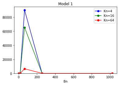
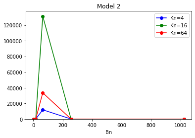
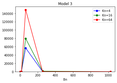
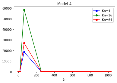
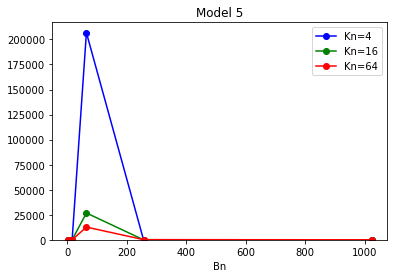
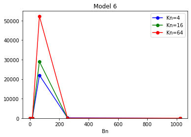
Figure 1: Comparison of different settings of $B_{n}$ and $K_{n}$ for all models, noise $5\%$ and sample size $n=200$

For all possibilities of $K_{n}$, the estimator has a very high error for $B_{n}=64$. For small $B_{n}$ of $1$ or $16$ and for high $B_{n}$ of $256$ or $1024$ the error is closer to zero. A closer look on the numbers shows that the error nevertheless varies between $0$ and $15$ with a tendency for smaller values of $B_{n}$ to show better performance. For different models, different values of $K_{n}$ are the best choice. This shows that the splitting of the sample procedure is indeed important for the performance of the estimator.

5 Proofs

5.1 Approximation error of shallow neural networks with random inner weights

The main trick in our results is the following approximation result for shallow neural networks with random inner weights and threshold squasher $\sigma(x)=1_{[0,\infty)}(x)$ as activation function. The proof relies on an extension of the approach in Barron (1994). Here condition (35) below will be used to show that for the logistic squasher $\sigma(x)=1/(1+\exp(-x))$ we have

$$\sigma\left(B_{n}\cdot(W_{k}^{T}X_{i}+T_{k})\right)\approx 1_{[0,\infty)}\left(W_{k}^{T}X_{i}+T_{k}\right).$$

Lemma 5.1.

Let $r>0$ and $\tilde{K}_{n}\in\mathbb{N}$ with $\tilde{K}_{n}\leq n$, and set $K_{n}=(\lceil\log n\rceil)^{4}\cdot\tilde{K}_{n}$. Let $m:\mathbb{R}^{d}\rightarrow\mathbb{R}$ be a function with

$$\int_{\mathbb{R}^{d}}|m(x)|\,dx<\infty,$$ (31)

and assume that the Fourier transform $\hat{F}$ of $m$ satisfies

$$|\hat{F}(\omega)|\leq\frac{c_{1}}{\|\omega\|^{d+1}\cdot(\log\|\omega\|)^{2}}\quad\mbox{for all }\omega\in\mathbb{R}^{d}\mbox{ with }\|\omega\|\geq 2$$ (32)

for some $c_{1}>0$. Let $(X,Y)$, $(X_{1},Y_{1})$, …, $(X_{n},Y_{n})$ be $\mathbb{R}^{d}\times\mathbb{R}$–valued random variables, and let $W_{1}$, …, $W_{K_{n}}$, $T_{1}$, …, $T_{K_{n}}$ be independent random variables, independent from $(X,Y)$, $(X_{1},Y_{1})$, …, $(X_{n},Y_{n})$, such that $W_{1}$, …, $W_{K_{n}}$ are uniformly distributed on $\{x\in\mathbb{R}^{d}\,:\,\|x\|=1\}$ and $T_{1}$, …, $T_{K_{n}}$ are uniformly distributed on $[-r,r]$. Then for $n$ sufficiently large, there exist (random)

$$\alpha_{0}\in[-c_{3},c_{3}]\quad\mbox{and}\quad\alpha_{1},\dots,\alpha_{K_{n}}\in\left[-\frac{c_{4}}{\tilde{K}_{n}},\frac{c_{4}}{\tilde{K}_{n}}\right],$$

which are independent of $(X,Y)$, $(X_{1},Y_{1})$, …, $(X_{n},Y_{n})$, such that outside of an event with probability less than or equal to

$$\exp\left(-\frac{1}{4}\cdot(\lceil\log n\rceil)^{2}\right)+\frac{1}{n},$$ (33)

we have

$$\int_{S_{r}}\left|m(x)-\alpha_{0}-\sum_{k=1}^{K_{n}}\alpha_{k}\cdot 1_{[0,\infty)}\left(W_{k}^{T}\cdot x+T_{k}\right)\right|^{2}{\mathbf{P}}_{X}(dx)\leq\frac{c_{22}}{\tilde{K}_{n}}$$ (34)

and

$$\min_{i=1,\dots,n,k=1,\dots,K_{n}:\atop\alpha_{k}\neq 0}|W_{k}^{T}X_{i}+T_{k}|\geq\delta_{n},$$ (35)

where $\delta_{n}=\frac{r}{n^{2}\cdot K_{n}}$.

Proof.

The complete proof of this result is found in the supplement. ∎

5.2 Outline of the proof of Theorem 2.1

In this subsection we give an outline of the proof of Theorem 2.1. The complete proof is given in the supplement.

W.l.o.g. we assume $\|m\|_{\infty}\leq\kappa_{n}$. Set $\tilde{K}_{n}=\lfloor K_{n}/(\lceil\log n\rceil)^{4}\rfloor$ and let $A_{n}$ be the event that $|Y_{i}|\leq\kappa_{n}$ holds for all $i\in\{1,\dots,n\}$ and that there exist (random)

$$\alpha_{0}\in[-c_{3},c_{3}]\quad\mbox{and}\quad\alpha_{1},\dots,\alpha_{K_{n}}\in\left[-\frac{c_{4}}{\tilde{K}_{n}},\frac{c_{4}}{\tilde{K}_{n}}\right],$$ (36)

which are independent of $(X,Y)$, $(X_{1},Y_{1})$, …, $(X_{n},Y_{n})$, such that (34) and

$$\min_{i=1,\dots,n,k=1,\dots,K_{n}:\atop\alpha_{k}\neq 0}\left|(\beta_{k}^{(0)})^{T}X_{i}+\gamma_{k}^{(0)}\right|\geq\delta_{n}$$ (37)

hold for $\delta_{n}=B_{n}\cdot\frac{\sqrt{d}}{n^{2}\cdot K_{n}}$, i.e., for $\delta_{n}=(\log n)^{2}$.

We have

$${\mathbf{E}}\int|m_{n}(x)-m(x)|^{2}{\mathbf{P}}_{X}(dx)$$

$$={\mathbf{E}}\left(\int|m_{n}(x)-m(x)|^{2}{\mathbf{P}}_{X}(dx)\cdot 1_{A_{n}}\right)+{\mathbf{E}}\left(\int|m_{n}(x)-m(x)|^{2}{\mathbf{P}}_{X}(dx)\cdot 1_{A_{n}^{c}}\right)$$

$$\leq{\mathbf{E}}\left(\int|m_{n}(x)-m(x)|^{2}{\mathbf{P}}_{X}(dx)\cdot 1_{A_{n}}\right)+4\kappa_{n}^{2}\cdot{\mathbf{P}}(A_{n}^{c})$$

$$=\mathbf{E}\Bigg{(}\bigg{(}\int|m_{n}(x)-m(x)|^{2}{\mathbf{P}}_{X}(dx)$$

$$\quad\quad\quad-2\cdot\bigg{(}\frac{1}{n}\sum_{i=1}^{n}|\tilde{m}_{n}(X_{i})-Y_{i}|^{2}\cdot 1_{\{|Y_{j}|\leq\kappa_{n}\,(j\in\{1,\dots,n\})\}}-\frac{1}{n}\sum_{i=1}^{n}|m(X_{i})-Y_{i}|^{2}\bigg{)}\bigg{)}\cdot 1_{A_{n}}\Bigg{)}$$

$$\quad+2\cdot{\mathbf{E}}\left(\bigg{(}\frac{1}{n}\sum_{i=1}^{n}|\tilde{m}_{n}(X_{i})-Y_{i}|^{2}\cdot 1_{\{|Y_{j}|\leq\kappa_{n}\,(j\in\{1,\dots,n\})\}}-\frac{1}{n}\sum_{i=1}^{n}|m(X_{i})-Y_{i}|^{2}\bigg{)}\cdot 1_{A_{n}}\right)$$

$$\quad+4\kappa_{n}^{2}\cdot{\mathbf{P}}(A_{n}^{c})$$

$$=:T_{1,n}+T_{2,n}+T_{3,n}.$$

Using results from empirical process theory together with bounds on the norm of the weights occuring during gradient descent we show in the supplement

$$T_{1,n}\leq c_{29}\cdot\frac{(\log n)^{3}\cdot K_{n}}{n}.$$

Furthermore we will use Lemma 5.1 to show

$$T_{3,n}\leq c_{30}\cdot\frac{(\log n)^{2}}{n}.$$

The remaining term we have to bound is $T_{2,n}$. Let $\alpha_{0}$ …$\alpha_{K_{n}}$ be defined as in (36) and define on $[0,1]$ a piecewise constant approximation of $m$ by

$$f(x)=\alpha_{0}+\sum_{k=1}^{K_{n}}\alpha_{k}\cdot 1_{[0,\infty)}\left(\sum_{j=1}^{d}w_{k,j}^{(0)}\cdot x^{(j)}+w_{k,0}^{(0)}\right).$$

Set

$$f^{*}(x)=\alpha_{0}+\sum_{k=1}^{K_{n}}\alpha_{k}\cdot\sigma\left(\sum_{j=1}^{d}w_{k,j}^{(0)}\cdot x^{(j)}+w_{k,1}^{(0)}\right).$$

For $g(x)=\alpha_{0}+\sum_{k=1}^{K_{n}}\alpha_{k}\cdot\sigma(\beta_{k}^{T}\cdot x+\gamma_{k})$ we define

$$\text{pen}(g)=\frac{c_{2}}{K_{n}}\cdot\sum_{k=0}^{K_{n}}(\alpha_{k})^{2}.$$

We will see that it is enough to show

$$F(\alpha^{(t_{n})},\beta^{(t_{n})},\gamma^{(t_{n})})-\frac{1}{n}\sum_{i=1}^{n}|Y_{i}-f^{*}(X_{i})|^{2}-\text{pen}(f^{*})$$

$$\leq c_{31}\cdot\frac{(\log n)^{3}\cdot K_{n}}{n},$$

where

$$F(\alpha,\beta,\gamma)=\frac{1}{n}\sum_{i=1}^{n}|Y_{i}-f_{net,(\alpha,\beta,\gamma)}(X_{i})|^{2}+\frac{c_{2}}{K_{n}}\cdot\sum_{k=0}^{K_{n}}(\alpha_{k})^{2}.$$

The main trick is to deduce via an elementary gradient descent analysis that on $A_{n}$

$$F(\alpha^{(t+1)},\beta^{(t+1)},\gamma^{(t+1)})-\frac{1}{n}\sum_{i=1}^{n}|Y_{i}-f^{*}(X_{i})|^{2}-{\text{p}en}(f^{*})$$

$$\leq\left(1-\frac{2\cdot c_{2}}{L_{n}\cdot K_{n}}\right)\cdot\left(F(\alpha^{(t)},\beta^{(t)},\gamma^{(t)})-\frac{1}{n}\sum_{i=1}^{n}|Y_{i}-f^{*}(X_{i})|^{2}-{\text{p}en}(f^{*})\right)$$

$$\quad+\frac{2\cdot c_{2}}{L_{n}\cdot K_{n}}\cdot\left(F(\alpha^{*},\beta^{(0)},\gamma^{(0)})-F(\alpha^{*},\beta^{(t)},\gamma^{(t)})\right),$$

for any $t\in\{1,\dots,t_{n}-1\}$ and $\alpha^{*}=(\alpha_{k})_{k=0,\dots,K_{n}}$ with $\alpha_{k}$ as defined above. If we now take advantage of the fact that in the logistic squasher the inner weights (which are not equal to zero) change only slightly, this implies

$$F(\alpha^{(t_{n})},\beta^{(t_{n})},\gamma^{(t_{n})})-\frac{1}{n}\sum_{i=1}^{n}|Y_{i}-f^{*}(X_{i})|^{2}-\text{pen}(f^{*})$$

$$\leq\left(1-\frac{2\cdot c_{2}}{L_{n}\cdot K_{n}}\right)^{t_{n}}\cdot\left(F(\alpha^{(0)},\beta^{(0)},\gamma^{(0)})-\frac{1}{n}\sum_{i=1}^{n}|Y_{i}-f^{*}(X_{i})|^{2}-\text{pen}(f^{*})\right)$$

$$\quad+t_{n}\cdot\frac{2\cdot c_{2}}{L_{n}\cdot K_{n}}\cdot c_{32}\cdot(\kappa_{n}+(\log n)^{4})\cdot c_{33}\cdot\frac{1}{n}$$

$$\leq\exp\left(-\frac{2\cdot c_{2}}{L_{n}\cdot K_{n}}\cdot t_{n}\right)\cdot F(\alpha^{(0)},\beta^{(0)},\gamma^{(0)})+c_{34}\cdot\frac{\kappa_{n}+(\log n)^{4}}{n}$$

$$\leq\exp(-c_{35}\cdot(\log n)^{2})\cdot c_{36}\cdot(\log n)^{2}+c_{37}\cdot\frac{\kappa_{n}+(\log n)^{4}}{n}\leq c_{38}\cdot\frac{(\log n)^{4}}{n}.$$

$\Box$

5.3 Proof of Corollary 2.1

It is well known that Lebesgue integrability and radial symmetry of $m$ imply radial symmetry of $|\hat{F}|$ (cf., Theorem 4.5.3 in Epstein (2008)). Then in Lemma 5.1 one can replace (32) by (23), where in the proof the radial symmetric density $g$ is defined by

$$g(t,\omega)=\begin{cases}\frac{1}{2r}\cdot\mathds{1}_{[-r,r]}(t)\cdot c_{39},\quad&\text{if}\ \|\omega\|\leq 1\\ \frac{1}{2r}\cdot\mathds{1}_{[-r,r]}(t)\cdot c_{39}\cdot\|\omega\|\cdot|\hat{F}(\omega)|,\quad&\text{if}\ \|\omega\|>1\end{cases}$$

with a suitable constant $c_{39}>0$. Now the proof of Corollary 1 is analogous to the proof of Theorem 2.1. $\Box$

5.4 Outline of the proof of Theorem 2.2

We set $p=d/2+1$, $M_{n}=\lceil n^{1/(2p+d)}\rceil$ and define

$$m^{(c_{n})}(x)=\sum_{j=1}^{M_{n}^{d}}c_{n,j}\cdot(\log n)^{-3}\cdot M_{n}^{-p}g(M_{n}(x-a_{n,j}))$$

as in the proof of Theorem 3.2 in Györfi et al. (2002). Here we choose $g$ so smooth that

$$|\hat{F}_{g}(\omega)|\leq\frac{c_{40}}{\|\omega\|^{d+1}\cdot(\log\|\omega\|)^{2}}\quad\mbox{for all }\omega\in\mathbb{R}^{d}\mbox{ with }\|\omega\|\geq 2$$

holds (cf., Remark 3). Let $\mathcal{C}_{n}$ be the set of all $(c_{n,j})_{j\in\{1,\dots,M_{n}^{d}\}}\in\{-1,1\}^{M_{n}^{d}}$, where

$$\left|\sum_{j=1}^{M_{n}^{d}}c_{n,j}\cdot\exp(i\omega^{T}a_{n,j})\right|\leq(\log n)\cdot M_{n}^{d/2}\quad(\omega\in\mathbb{R}^{d}\setminus\{0\})$$

holds. If $c_{n}=(c_{n,j})_{j}\in\mathcal{C}$ we can show that

$$|\hat{F}_{m^{(c_{n})}}(\omega)|\leq\frac{c_{1}}{\|\omega\|^{d+1}\cdot(\log\|\omega\|)^{2}}\quad\mbox{for all }\omega\in\mathbb{R}^{d}\mbox{ with }\|\omega\|\geq 2.$$

Let $X,N,C_{n}$ be independent with $X\sim U([0,1]^{d})$, $N\sim\mathcal{N}(0,1)$ and $C_{n}\sim U(\mathcal{C}_{n})$. Arguing as in the proof of Theorem 3.2 in Györfi et al. (2002) we can bound

$$\inf_{\hat{m}_{n}}\sup_{(X,Y)\in\mathcal{D}}{\mathbf{E}}\int|\hat{m}_{n}(x)-m(x)|^{2}{\mathbf{P}}_{X}(dx)$$

$$\geq c_{41}\cdot(\log n)^{-6}\cdot n^{-\frac{2p}{2p+d}}-4\cdot\|g\|_{\infty}^{2}\cdot{\mathbf{P}}\{C_{n}\notin\mathcal{C}_{n}\}.$$

The result follows from the definition of $p$ and an application of Hoeffding’s inequality, which yields

$${\mathbf{P}}\{C_{n}\notin\mathcal{C}_{n}\}\leq\frac{c_{42}}{n}.$$

$\Box$

5.5 Outline of the proof of Theorem 3.1

W.l.o.g. we assume $\|m\|_{\infty}\leq\kappa_{n}$. Set $\tilde{K}_{n}=\lfloor K_{n}/(\lceil\log n\rceil)^{4}\rfloor$ and let $A_{n}$ be the event that $|Y_{i}|\leq\kappa_{n}$ holds for all $i=1,\dots,n$ and that there exist (random)

$$\alpha_{0}\in[-c_{3},c_{3}]\quad\mbox{and}\quad\alpha_{1},\dots,\alpha_{K_{n}}\in\left[-\frac{c_{4}}{\tilde{K}_{n}},\frac{c_{4}}{\tilde{K}_{n}}\right],$$

which are independent of $(X,Y)$, $(X_{1},Y_{1})$, …, $(X_{n},Y_{n})$, such that (34) and (37) hold for $\delta_{n}=B_{n}\cdot\frac{\sqrt{d}}{n^{2}\cdot K_{n}}$, i.e., for $\delta_{n}=(\log n)^{2}$. Furthermore, define $f^{*}$ as in the proof of Theorem 2.1.

As in the proof of Theorem 2.1 we get

$${\mathbf{E}}\int|m_{n}(x)-m(x)|^{2}{\mathbf{P}}_{X}(dx)$$

$$\leq\mathbf{E}\Bigg{(}\bigg{(}\int|m_{n}(x)-m(x)|^{2}{\mathbf{P}}_{X}(dx)$$

$$\quad-2\cdot\bigg{(}\frac{1}{n}\sum_{i=1}^{n}|\tilde{m}_{n}(X_{i})-Y_{i}|^{2}\cdot 1_{\{|Y_{j}|\leq\kappa_{n}\,(j\in\{1,\dots,n\})\}}-\frac{1}{n}\sum_{i=1}^{n}|m(X_{i})-Y_{i}|^{2}\bigg{)}\bigg{)}\cdot 1_{A_{n}}\Bigg{)}$$

$$\quad+2\cdot{\mathbf{E}}\left(\bigg{(}\frac{1}{n}\sum_{i=1}^{n}|\tilde{m}_{n}(X_{i})-Y_{i}|^{2}\cdot 1_{\{|Y_{j}|\leq\kappa_{n}\,(j\in\{1,\dots,n\})\}}-\frac{1}{n}\sum_{i=1}^{n}|m(X_{i})-Y_{i}|^{2}\bigg{)}\cdot 1_{A_{n}}\right)$$

$$\quad+4\kappa_{n}^{2}\cdot{\mathbf{P}}(A_{n}^{c})$$

$$=:T_{1,n}+T_{2,n}+T_{3,n}.$$

Standard results from empirical process theory enable us to show

$$T_{1,n}\leq\frac{c_{43}\cdot(\log n)^{2}\cdot\left((K_{n}+1)\cdot(\log n)+1\right)}{n}\leq c_{44}\cdot\frac{(\log n)^{3}\cdot K_{n}}{n}.$$

As in the proof of Theorem 2.1 application of Lemma 5.1 yields

$$T_{3,n}\leq c_{45}\cdot\frac{(\log n)^{2}}{n}.$$

Hence again it will be sufficient to derive a bound on $T_{2,n}$, and as in the proof of Theorem 2.1 the crucial step will be to bound on the event $A_{n}$

$$\frac{1}{n}\sum_{i=1}^{n}|\tilde{m}_{n}(X_{i})-Y_{i}|^{2}-\frac{1}{n}\sum_{i=1}^{n}|f^{*}(X_{i})-Y_{i}|^{2}.$$

But this is quite simple here as by definition of $\tilde{m}_{n}$ as a least squares estimator this term is less than or equal to zero. $\Box$

References

- [1] Allen-Zhu, Z., Li, Y., and Liang, Y. (2019). Learning and generalization in overparameterized neural networks, going beyond two layers. In Advances in Neural Information Processing Systems, 32.
- [2] Allen-Zhu, Z., Li, Y., and Song, Z. (2019). A convergence theory for deep learning via over-parameterization. In International Conference on Machine Learning, 97, pp. 242-252.
- [3] Andoni, A., Panigraphy, R., Valiant, G., and Zhang, L.(2014). Learning polynomials with neural networks. In International Conference on Machine Learning, pp. 1908 –1916.
- [4] Arora, S., Cohen, N., Golowich, N., and Hu, W. (2018). A convergence analysis of gradient descent for deep linear neural networks. In International Conference on Learning Representations.
- [5] Arora, S., Du, S., Hu, W., Li, Z., Salakhutdinov, R., and Wang, R. (2019a). On exact computation with an infinitely wide neural net. In Advances in Neural Information Processing Systems, 32.
- [6] Arora, S., Du, S., Hu, W., Li, Z., and Wang, R. (2019b). Fine-grained analysis of optimization and generalization for overparameterized two-layer neural networks. In International Conference on Machine Learning, 97, pp. 322-332.
- [7] Bagirov, A. M., Clausen, C., and Kohler, M. (2009). Estimation of a regression function by maxima of minima of linear functions. IEEE Transactions on Information Theory 55: 833-845.
- [8] Barron, A. R. (1993). Universal approximation bounds for superpositions of a sigmoidal function. IEEE Transactions on Information Theory 39: 930–944.
- [9] Barron, A. R. (1994). Approximation and estimation bounds for artificial neural networks. Machine Learning 14: 115-133.
- [10] Bartlett, P., Harvey, N., Liaw, C., and Mehrabian, A. (2019). Nearly-tight VC-dimension bounds for piecewise linear neural networks. Journal of Machine Learning Research 20:1–17.
- [11] Bauer, B., and Kohler, M. (2019). On deep learning as a remedy for the curse of dimensionality in nonparametric regression. Annals of Statistics 47: 2261–2285.
- [12] Braun, A., Kohler, M., and Walk, H. (2019). On the rate of convergence of a neural network regression estimate learned by gradient descent. Preprint, arXiv: 1912.03921.
- [13] Brutzkus, A., Globerson, A., Malach, E., and Shalew-Shwartz S. (2018). SGD learn overparametrized networks that provably generalize on linearly seperable data. In International Conference on Learning Representation
- [14] Choromanska, A., Henaff, M., Mathieu, M., Arous, G. B., and LeCun, Y. (2015) The loss surface of multilayer networks. In International Conference on Artificial Intelligence and Statistics, 38, pp. 192-204.
- [15] Du, S., and Lee, J. (2018). On the power of over-parametrization in neural networks with quadratic activation. In International Conference on Machine Learning, 80, pp. 1329-1338.
- [16] Du, S., Lee, J., Li, H., Wang, L., und Zhai, X. (2019). Gradient descent finds global minima of deep neural networks. In International Conference on Machine Learning, pp. 1675-1685.
- [17] Dudek, G. (2019). Generating random weights and biases in feedfoward neural networks with random hidden nodes. Information Sciences, 481(C): 33-56.
- [18] Epstein, Ch. L. (2008). Introduction to the Mathematics of Medical Imaging. 2nd edition, SIAM. Society for Industrial and Applied Mathematics. Philadelphia.
- [19] Ghorbani, B., Mei, S., Misiakiewicz, T. and Montanari, A. (2019). Limitations of lazy training of two-layer neural networks. In Advances in Neural Information Processing Systems, 32.
- [20] Gonon, L. (2021). Random feature neural networks learn Black-Scholes type PDEs without curse of dimensionality. Preprint, arXiv: 2106.08900.
- [21] Gonon, L., Grigoryeva, L., and Ortega, J.-P. (2023). Approximation bounds for random neural networks and reservoir systems. The Annals of Applied Probability, 33(1): 28–69.
- [22] Goodfellow, I., Bengio, Y., and Courville, A. (2016). Deep Learning. MIT Press, Cambridge, Massachusetts.
- [23] Györfi, L., Kohler, M., Krzyżak, A., and Walk, H. (2002). A Distribution–Free Theory of Nonparametric Regression. Springer, New York.
- [24] Huang, G.-B., Chen, L., and Siew, C.-K. (2006). Universal approximation using incremental contractive feedforward networks with random hidden nodes. IEEE Transactions on Neural Networks 17: 879-892.
- [25] Igelnik, B. and Pao, Y.-H. (1995). Stochastic choice of basis functions in adaptive function approximation and the functional-link net. IEEE Transactions on Neural Networks, 6: 1320 -1329.
- [26] Imaizumi, M., and Fukamizu, K. (2018). Deep neural networks learn non-smooth functions effectively. In International Conference on Artificial Intelligence and Statistics, pp. 869-878.
- [27] Jacot, A., Gabriel, F., und Hongler, C. (2020). Neural Tangent Kernel: Convergence and Generalization in Neural Networks. In Advances in Neural Information Processing Systems, 31.
- [28] Javanmard, A., Mondelli, M., and Montanari, A. (2021). Analysis of two-layer neural network via displacement convexity. Annals of Statistics, 48(6): 3619-3642.
- [29] Kawaguchi, K. (2016). Deep learning without poor local minima. Advances in Neural Information Processing Systems, 29.
- [30] Kawaguchi, K, and Huang, J. (2019). Gradient descent finds global minima for generalizable deep neural networks of practical sizes. In 2019 57th annual allerton conference on communication, control, and computing (Allerton), pp. 92–99.
- [31] Kim, Y. (2014). Convolutional Neural Networks for Sentence Classification. In Empirical Methods in Natural Language Processing, pp. 1746–-1751.
- [32] Kohler, M., and Krzyżak, A. (2017). Nonparametric regression based on hierarchical interaction models. IEEE Transaction on Information Theory 63: 1620-1630.
- [33] Kohler, M., and Krzyżak, A. (2021). Over-parametrized deep neural networks minimizing the empirical risk do not generalize well. Bernoulli 27(4): 2564-2597.
- [34] Kohler, M., Krzyżak, A., and Langer, S. (2022). Estimation of a function of low local dimensionality by deep neural networks. IEEE Transactions on Information Theory 68(6): 4032 – 4042.
- [35] Kohler, M., and Langer, S. (2022). Discussion of “Nonparametric regression using deep neural networks with ReLU activation function”. Annals of Statistics 48(4): 1906-1910.
- [36] Kohler, M., and Langer, S. (2022). On the rate of convergence of fully connected very deep neural network regression estimates using ReLU activation functions. Annals of Statistics 49(4): 2231–2249.
- [37] Koltchinskii, V. (2006). Local Rademacher complexities and oracle inequalities in risk minimization. Annals of Statistics 34(6):2593 – 2656.
- [38] Krizhevsky, A., Sutskever, I., and Hinton, G. E. (2012). ImageNet classification with deep convolutional neural networks. In Advances In Neural Information Processing Systems 25, pp. 1097–1105.
- [39] Kůrková, V., and Sanguinetti, M. (2008). Geometric upper bounds on rates of variable-basis approximation. IEEE Transactions on Information Theory 54: 5681 – 5688.
- [40] Lee, W.S. (1996). Agnostic Learning and Single Hidden Layer Neural Networks. PhD Thesis, Australian National University.
- [41] Liang, S., Sun, R., Lee, J., and Srikant, R. (2018). Adding one neuron can eliminate all bad local minima. Advances In Neural Information Processing Systems, pp. 4355 – 4365.
- [42] Li, Y., and Liang, Y. (2018). Learning overparameterized neural networks via stochastic gradient descent on structured data. In Advances in Neural Information Processing Systems, pp. 8168- 8177.
- [43] McCaffrey, D. F., and Gallant, A. R. (1994). Convergence rates for single hidden layer feedforward networks. Neural Networks 7: 147-158.
- [44] Pisier, G. ”Remarques sur un resultat non publie de B. Maurey,” presented at the Seminaire d’analyse fonctionelle 1980-1981, Ecole Polytechnique, Centre de Mathematiques, Palaiseau.
- [45] Poggio, T., Banburski, A. , and Liao,Q. Theoretical issues in deep networks. Proceedings of the National Academy of Sciences 117: 30039–30045.
- [46] Rahimi, A., and Recht, B. (2009). Weighted sums of random kitchen sinks: Replacing minimization with randomization in learning. In Advances in Neural Information Process Systems 21, pp. 1313-1320.
- [47] Schmidt-Hieber, J. (2020). Nonparametric regression using deep neural networks with ReLU activation function (with discussion). Annals of Statistics 48(4): 1875–1897.
- [48] Silver, D., Schrittwieser, J., Simonyan, K., Antonoglou, I., Huang, A., Guez, A., Huber, T., et al. (2017). Mastering the game of go without human knowledge. Nature 550: 354-359.
- [49] Sitzmann, V., Martel, J., Bergman,A., Lindell, D., and Wetzstein, G. (2020). Implicit neural representations with periodic activation functions. In Advances in Neural Information Processing Systems 33, pp. 7462–7473.
- [50] Sonoda, S., Ishikawa, I., and Ikeda, M. (2021). Ridge regression with overparametrized two-layer networks convergence to ridgelet spectrum. International Conference on Artificial Intelligence and Statistics 130, pp. 2674 – 2682.
- [51] Stone, C. J. (1982). Optimal global rates of convergence for nonparametric regression. Annals of Statistics 10(4): 1040-1053.
- [52] Suzuki, T., and Nitanda, A. (2021). Deep learning is adaptive to intrinsic diemsnionality of model smoothness in anisotropic Besov space. Advances in Neural Information Processing Systems 34, pp. 3609-3621.
- [53] Widrow, B., Greenblatt, A., Kim, Y., and Park, D. (2013). The No-Prop algorithm: A new learning algorithm for multilayer neural networks. Neural Networks 37: 182-188.
- [54] Woodworth, B., Gunasekar, S., Lee, J., Moroshko, E., Savarese, P., Golan, I., Soudry, D., und Srebro, N. (2020). Kernel and rich regimes in overparametrized models. In Conference on Learning Theory 125, pp. 3635–3673.
- [55] Wu, Y., Schuster, M., Chen, Z., Le, Q., Norouzi, M., Macherey, W., Krikum, M., et al. (2016). Google’s neural machine translation system: Bridging the gap between human and machine translation. arXiv: 1609.08144.
- [56] Yosida, K. (1968). Functional Analysis. 2nd edition. Springer. Berlin.
- [57] Zou, D., Cao, Y., Zhou, D., und Gu, Q. (2020). Gradient descent optimizes over-parameterized deep ReLU networks. Machine Learning 109: 467 – 492.