AGN Jets and Winds in Polarised Light: The Case of Mrk 231

Abstract

We present the results of a multi-frequency, multi-scale radio polarimetric study with the Very Large Array (VLA) of the Seyfert 1 galaxy and BALQSO, Mrk 231. We detect complex total and polarized intensity features in the source. Overall, the images indicate the presence of a broad, one-sided, curved outflow towards the south which consists of a weakly collimated jet with poloidal inferred magnetic fields, inside a broader magnetized “wind” or “sheath” component with toroidal inferred magnetic fields. The model of a kpc-scale weakly collimated jet/lobe in Mrk 231 is strengthened by its C-shaped morphology, steep spectral index throughout, complexities in the magnetic field structures, and the presence of self-similar structures observed on the 10-parsec-scale in the literature. The “wind” may comprise both nuclear starburst (close to the core) and AGN winds, where the latter maybe the primary contributor. Moving away from the core, the “wind” component may also comprise the outer layers (or “sheath”) of a broadened jet. The inferred value of the (weakly collimated) jet production efficiency, $\eta_{\mathrm{jet}}\sim$0.01 is consistent with the estimates in the literature. The composite jet and wind outflow in Mrk 231 appears to be low-power and matter-dominated, and oriented at a small angle to our line of sight.

1 Introduction

Active galactic nuclei (AGN) are powered by the release of gravitational energy as matter is accreted onto supermassive ($10^{6}-10^{10}$ M_☉) black holes. Seyfert galaxies are a sub-class of AGN, mostly hosted by spiral or lenticular galaxies. They are typically classified as “radio-quiet” AGN as their “radio-loudness” parameter $R\equiv\mathrm{S_{radio}/S_{optical}}$ is often less than 10 (Kellermann et al., 1989); S is the flux density at radio (5 GHz) and optical (B-band) frequencies. Many Seyfert galaxies however do not adhere to the formal dividing line and move into the “radio-loud” category when the galactic optical contribution is properly accounted for (e.g., Ho & Peng, 2001; Kharb et al., 2012). Seyferts have been further classified as type 1 or type 2 depending on the presence of broad and narrow emission lines versus only narrow emission lines (Antonucci, 1993).

The origin of radio outflows in Seyfert galaxies is still a matter of debate, with AGN jets/winds and starburst superwinds being the primary contenders (Ulvestad et al., 1981; Baum et al., 1993; Colbert et al., 1996; Panessa et al., 2019). Sebastian et al. (2019b, a, 2020) have used radio polarimetry to compare the radio outflows of Seyfert galaxies to starburst galaxies and found suggestions of differences in their degree of polarization. Silpa et al. (2021) have deduced that the Seyfert 1 galaxy III Zw 2 harbours a composite jet and wind outflow exhibiting toroidal inferred magnetic (B-) fields, from their radio polarimetric study.

Mrk 231 (aka UGC 8058 or VII Zw 490) at a redshift of 0.04217 is a well-studied Seyfert type 1 galaxy (Sanders et al., 1988b; Surace et al., 1998). In fact this optically identified source is known to be the most luminous object in the local ($z<0.1$) Universe (Sanders et al., 1988b). It has alternately been classified as a Broad Absorption Line Quasi Stellar Object (BALQSO; Boksenberg et al., 1977; Smith et al., 1995; Gallagher et al., 2002), and an Ultra Luminous InfraRed Galaxy (ULIRG; Sanders et al., 1988a). The synchrotron emission from Mrk 231 is known to be variable on a timescale of a few days (McCutcheon & Gregory, 1978) to years (Condon et al., 1991). Mrk 231 contains an OH megamaser (Baan, 1985) as well as a massive starburst (Neff & Ulvestad, 1988). Very Long Baseline Array (VLBA) observations of Mrk 231 have revealed a triple radio source $\sim 2$ parsec in extent, with a PA $\sim 5\degr$ (Ulvestad et al., 1999a).

Mrk 231 exhibits AGN-driven outflows in multiple gas phases (Feruglio et al., 2015) and over multiple spatial scales (e.g., Veilleux et al., 2016). The presence of a parsec-scale AGN jet and a BAL wind has been documented by Reynolds et al. (2009). The study by Rupke & Veilleux (2011) reveals the presence of an AGN-driven wind, starburst-driven wind and a radio jet in Mrk 231. Veilleux et al. (2016) suggest that Mrk 231 is the nearest example of weak-lined “wind-dominated” quasars with high accretion rates. The morphology and kinematics of the neutral atomic and molecular gas outflows as presented by Feruglio et al. (2015); Rupke & Veilleux (2013); Rupke et al. (2017) point to a cold gas “wide angle outflow” on $\sim 1-20$ kpc scales. The co-existence of a radio jet and powerful multi-phase outflows in Mrk 231 (Reynolds et al., 2009, 2017) make it an ideal candidate to study the origin of outflows in AGN.

We present here radio polarimetric observations of Mrk 231 at multiple frequencies and resolutions with the Very Large Array (VLA). In this paper, we adopt a cosmology with H₀ = 73 km s^-1 Mpc^-1, $\Omega_{m}$ = 0.27, $\Omega_{v}$ = 0.73. The spectral index $\alpha$ is defined such that $S_{\nu}\propto\nu^{\alpha}$, S_ν being the flux density at frequency $\nu$.

Table 1: Observation details

VLA Array	Frequency	Observation	Resolution
Configuration	(GHz)	Period	(arcsec)
A	1.4	1995 July 3 $-$ July 4	1.2
C	1.4	1996 Feb 17	13.4
D	1.4	1995 May 12 $-$ June 2	40.2
A	4.9	1995 July 21 $-$ July 22	0.3
B	4.9	1995 Nov 2	1.2
C	4.9	1996 Feb 17	4.0
D	4.9	1995 May 3 $-$ May 24	11.9

2 Radio Data Analysis

We observed Mrk 231 with the VLA at 1.4 and 4.9 GHz in the A, B, C, and D-array configurations during 1995 - 1996 (Project ID: AB740). Table 1 provides the details of the observations. 3C286 and 3C48 were used as the primary flux density as well as the polarisation calibrators, while J1400+621 was used as the phase calibrator for the whole experiment. The data were processed with AIPS using standard imaging and self-calibration procedures. AIPS task PCAL was used to solve for the antenna “leakage” terms (D-terms) as well as polarisation of the calibrators 3C286 and 3C48. The leakage amplitudes were typically a few percent. Polarisation calibration of the 4.9 GHz A-array data was unsuccessful.

The polarisation intensity (PPOL) and polarisation angle (PANG) images were created by first running the AIPS task IMAGR for Stokes ‘Q’ and ‘U’ and then combining these images using the task COMB. Pixels with intensity values below 3$\sigma$ and angle errors $>10\degr$ were blanked before making PPOL and PANG images, respectively. (The cut on the angle error was relaxed to 15$\degr$ for the 1.4 GHz A-array image.) Fractional polarisation images were created using the PPOL and total intensity images where pixels with $>10\%$ errors were blanked.

We created two two-frequency spectral index images using the AIPS task COMB after convolving images at both frequencies with the same circular beams (1.5$\arcsec$ and 15.0$\arcsec$). Pixels with total intensity value below 3$\sigma$ were blanked before making the spectral index images. Rotation measure (RM) images were created using three frequencies with AIPS tasks MCUBE, TRANS, and RM. For this, we split the two IF data at L-band (IF1 = 1.465 GHz, IF2 = 1.385 GHz) and used the C-band (frequency = 4.860 GHz) data as such. Two RM images were made after convolving all images with the same circular beam (1.5$\arcsec$ and 15.0$\arcsec$).

Flux density values reported in the paper were obtained using the Gaussian-fitting AIPS task JMFIT for compact components like the core, and AIPS task TVSTAT for extended emission. The rms noise values were similarly obtained using AIPS tasks TVWIN and IMSTAT.

Figure 1: 4.86 GHz VLA B-array total intensity contour image with electric polarisation vectors in red. Contour levels are in percentage of peak surface brightness (=250.2 mJy beam^-1) and increase in steps of 2, with the lowest contour level being at $\pm 0.021$%. Polarization vector of length 1$\arcsec$ corresponds to fractional polarization of 41.7%.

3 Results

3.1 Radio morphology

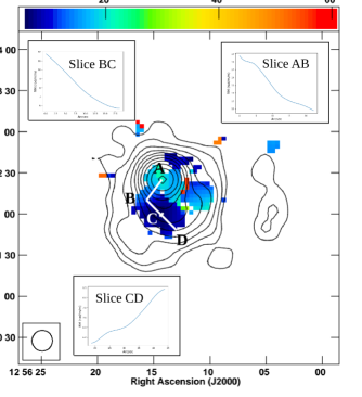
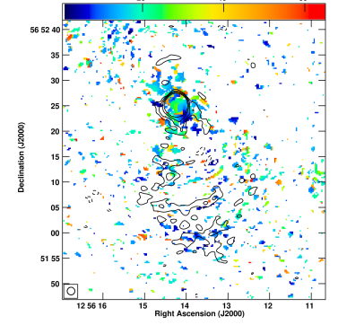
Figure 6: The $1.4-4.9$ GHz rotation measure image of Mrk 231. Left: 15$\arcsec$ resolution image. Contour levels are in percentage of peak surface brightness (=252.7 mJy beam^-1), with contours levels increasing in steps of 2, with the lowest contour level being $\pm 0.085$%. The color scale extends from 5.27 to 60.58 rad m^-2. Right: $1.5\arcsec$ resolution image. Contour levels are in percentage of peak surface brightness (=232.3 mJy beam^-1), with contours levels increasing in steps of 2, with the lowest contour level being $\pm 0.042$%. The color scale extends from 0.55 to 64.78 rad m^-2.

A bright core and fainter emission with a north-south orientation, extending to $\sim$4 kpc south from the core, is detected in the 4.9 GHz B-array VLA image of Mrk 231 (Figure 1). The 1.4 GHz A-array image reveals a $\sim$ 25 kpc-scale poorly collimated, filamentary radio structure to the south, extending beyond the optical emission of the host galaxy (Figure 2, left panel). See also the VLA 1.4 GHz A-array image of Mrk 231 in Morganti et al. (2016). Specifically, the resemblance of Fig. 2 left in the current work to Fig. 6 in Morganti et al. (2016) suggests that the lobe morphology is real, and not completely affected by imaging artefacts, although some of the “ribbed” features might indeed by artefacts since we see them on the counter-lobe side. Similar filamentary radio lobes have been observed in other Seyfert galaxies (e.g., NGC 3079; Sebastian et al., 2019b). The 4.9 GHz C-array image reveals diffuse lobe-like emission to the south that extends to $\sim$ 30 kpc (Figure 2, right panel), which was also detected in the 1.4 GHz images of Ulvestad et al. (1999a). The 1.4 GHz C-array and 4.9 GHz D-array images reveal significant amounts of diffuse emission around the core and diffuse lobe-like emission extending $\sim$55 kpc to the south (Figure 3). The 4.9 GHz D-array image also shows an extension towards the north. The broad radio structures seen towards the south in Figure 3 encompasses the radio structures revealed in Figure 2.

The left panel of Figure 4 shows that the region where the outflow in the 1.4 GHz A-array image de-collimates and spreads out to the south-west, coincides with the edge of the optical diffuse emission. The outflow in the 1.4 GHz C-array image also shows a broad curvature towards the west, which in fact, coincides with the direction of the bending of the tidal arm in the south (Figure 4, right panel). The morphology and the extent of the radio structure in the 1.4 GHz C-array image resemble the WSRT image presented in Morganti et al. (2016). The 1.4 GHz D-array image in Figure 5 is the lowest resolution image of Mrk 231 from the current project. The extent of the radio structure in this image is $\sim 3\arcmin$ ($\sim 145$ kpc). Reynolds et al. (2009) have deduced that the outflow inclination is small on the basis of slow Very Long Baseline Array (VLBA) speeds. This is consistent both with its BALQSO nature as well as its kpc-scale morphology as seen in the left panel of Figure 3. The 4.9 GHz A-array image reveals only a radio core.

Based on our multi-resolution images we find that the kpc-scale radio structure to the south in Mrk 231 resembles a “flaring jet” or lobe, rather than a radio “bubble”. Flaring jets leading into lobes are typically observed in Fanaroff-Riley type I (FRI) radio galaxies (e.g., Bondi et al., 2001; Laing & Bridle, 2002). The radio structure is one-sided and C-shaped (see Figure 3, left), and shows directionality rather than spherical symmetry expected from a bubble. The spectral index images do not show any change in values but is steep spectrum throughout. For instance, a spectral index flattening is observed at the edges of the radio bubbles in the Seyfert galaxy NGC 6764 (Hota & Saikia, 2006; Kharb et al., 2010). It is interesting to note that the 10-kpc-scale and the 10-parsec-scale radio structures in Mrk 231 appear to be “self-similar” (see Figure 1 in Morganti et al., 2016), reminiscent of the lobes observed in Mrk 6 (Kharb et al., 2006). In the case of Mrk 231, the radio structures on the two scales are not as clearly delineated, most likely due to their orientation being close to our line of sight. The presence of the two distinct structures may even be consistent with episodic jet activity in Mrk 231, like in Mrk 6, but cannot be confirmed without additional spectral index data on multiple scales. Thus, based on the observational evidence, we have adopted the interpretation that we see a weakly collimated jet on the kpc scale. With this general scenario in mind, we have estimated the “jet power” of Mrk 231 in Section 3.5.1 ahead.

3.2 Polarization structures

Complex polarization structures are revealed in the VLA images. Figures 1 $-$ 3 and 5, which are presented in the decreasing order of resolution, show the polarization electric ($\chi$) vectors as red ticks with lengths proportional to linear fractional polarization. The rotating $\chi$ vectors (with errors of a few degrees) at the core edges in Figure 1 suggest tangential or compressed B-fields, assuming optically thin emission.

The kpc-scale weakly collimated jet in the south shows low levels of polarization in the higher resolution 1.4 GHz A-array image (Figure 2, left panel) whereas strong polarization in the lower resolution 4.9 GHz C-array image (Figure 2, right panel). This can be explained as an effect of wavelength-dependent depolarization at 1.4 GHz (Burn, 1966). We find four distinct polarized regions along the weakly collimated jet in the 1.4 GHz A-array image. The regions closer to the core exhibit inferred B-fields parallel to the local jet direction whereas the regions further away exhibit inferred B-fields aligned with the lobe edges, assuming optically thin emission. The 4.9 GHz C-array image also reveals inferred B-fields aligned with the outer-edges of the lobe and a region closer to the core with inferred B-fields parallel to the local jet direction. It also reveals a region to the west of the core with inferred transverse B-fields. The lower polarization of the core in the 4.9 GHz C-array image as compared to the 1.4 GHz A-array image can be explained as a beam depolarization effect.

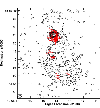
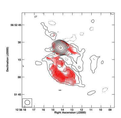
Figure 2: Left: 1.42 GHz VLA A-array total intensity contour image with electric polarisation vectors in red. Contour levels are in percentage of peak surface brightness (=230.95 mJy beam^-1), with contours levels increasing in steps of 2, with the lowest contour level being $\pm 0.020$%. Polarization vector of length 1$\arcsec$ corresponds to fractional polarization of 20%. Right: 4.86 GHz VLA C-array total intensity contour image with polarisation vectors in red. Contour levels are in percentage of peak surface brightness (=258.3 mJy beam^-1), with contours levels increasing in steps of 2, with the lowest contour level being $\pm 0.042$%. Polarization vector of length 1$\arcsec$ corresponds to fractional polarization of 12.5%.

The B-field structure in the 1.4 GHz C-array image is not representative of a typical “bubble” with aligned fields at the edges, but rather shows complexities. The 4.9 GHz D-array image reveals three distinct regions of ordered B-fields in the southern side and two distinct regions of ordered B-fields in the northern side of the core (Figure 3, right panel). The transverse inferred B-fields in the core of the 4.9 GHz B-array image continues all the way up to the edge of the lobe as seen in the 1.4 GHz C-array and 4.9 GHz D-array images. The B-fields in the 1.4 GHz C-array image also clearly follow the curvature (C-shape) in the lobe, similar to that observed in the south-western lobe of III Zw 2 (Silpa et al., 2021). The 1.4 GHz D-array image reveals ordered B-fields at the centre and aligned fields at the edges (Figure 5). We also note that had the kpc-scale radio structure been a typical radio “bubble”, different resolution images at the same frequency would have yielded similar polarization structures except for differences arising from beam depolarization effects, which is not the case of Mrk 231.

The total flux density, polarized flux density, fractional polarization (F.P) and polarization angle values for different radio components of Mrk 231 at different resolutions are summarized in Table 2. The F.P values in the outflow (jet and jet+wind) are typically $40-50$% in the higher resolution images and $20-30$% in the lower resolution images at both frequencies. The F.P value for the composite core+jet+wind radio structure in the D-array 1.4 GHz image is $\sim 17\%$.

3.3 A rotation measure analysis

The $1.4-4.9$ GHz rotation measure (RM) images of Mrk 231 at resolutions of 15$\arcsec$ and 1.5$\arcsec$ are presented in the left and right panels of Figure 6, respectively. The mean RM values are $14\pm 2$ and $20\pm 4$ rad m^-2 (errors are obtained using error propagation rules) in the 15 arcsec image and 1.5 arcsec image, respectively. The three inlayed plots in the left panel of Figure 6 present the radial RM profiles along the slices AB, BC and CD. The RM is given by the following relation:

$$\mathrm{RM=\int 812\,n_{e}\,B_{||}\,dl~{}~{}~{}rad~{}m^{-2}},$$ (1)

where n_e is the electron number density of the Faraday rotating medium in cm^-3, B_|| is the line-of-sight component of the B-field in milliGauss (mG) and dl is the path length of the Faraday screen in parsecs (pc). Based on the above relation, the radial RM profile can translate to a radial electron number density (n_e) profile of the Faraday rotating medium through which the jet passes, assuming a constant B_|| field and that the Faraday rotating medium has the same B-field as the radio source. We also assume that internal Faraday rotation is not a significant contributor. The B_|| field could be taken as the equipartition field of $\sim 3\times 10^{-3}$ mG (using the weakly collimated jet/lobe in 4.9 GHz C-array image).

Using the PYTHON fitting procedure CURVE$\_$FIT, we obtain the following best fitting power-laws for the radial RM profiles, or equivalently the radial n_e profiles: n_e $\propto$ RM $\propto$ r^a, where a = $-0.11$, $-0.17$ and 0.49 for slices AB, BC and CD respectively. Here, r is the radial distance from the core for slice AB and from the point B for slices BC and CD. The three slices were chosen on the basis of a drastic change in the RM profile, as well as the direction of the weakly collimated jet. The pressure profile of the external medium could be inferred from the n_e profile as p_gas $\propto$ n${}_{\mathrm{e}}^{\gamma}$, assuming adiabatic equation of state for non-relativistic mono-atomic gas and $\gamma$ = 5/3 being the ratio of specific heats (Park et al., 2019). Therefore, we infer p_gas $\propto$ r^b, where b = $-0.18$, $-0.28$ and 0.82 for slices AB, BC and CD respectively.

We know that the magnetic pressure, p_mag is B²/8$\pi$. The poloidal B-field varies as r^-2 and the toroidal B-field varies as r^-1 v^-1 (Begelman et al., 1984). The magnetization parameter, $\beta$, is given as the ratio of gas pressure to magnetic pressure, i.e.

$$\mathrm{\beta=p_{gas}/p_{mag}}.$$ (2)

For poloidal B-fields, we find that $\beta$ $\propto$ r^c, where c = 3.8, 3.7 and 4.8 for slices AB, BC and CD respectively. For toroidal B-fields, we find that $\beta$ $\propto$ r^d, where d = 1.8, 1.7 and 2.8 for slices AB, BC and CD respectively. Thus, for both poloidal and toroidal B-fields, the value of $\beta$ increases with distance from the core. We use this information to infer that the outflow is matter-dominated as discussed ahead in Section 4.6. One caveat in this analysis is the assumption of self-similarity, which may be too simplistic for this complex system.

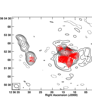
Figure 3: Left: 1.42 GHz VLA C-array total intensity contour image with electric polarisation vectors in red. Contour levels are in percentage of peak surface brightness (=252.1 mJy beam^-1), with contours levels increasing in steps of 2, with the lowest contour level being $\pm 0.17$%. Polarization vector of length 1$\arcsec$ corresponds to fractional polarization of 3.7%. Right: 4.86 GHz VLA D-array total intensity contour image with polarisation vectors in red. Contour levels are in percentage of peak surface brightness (=270.2 mJy beam^-1), with contours levels increasing in steps of 2, with the lowest contour level being $\pm 0.021$%. Polarization vector of length 1$\arcsec$ corresponds to fractional polarization of 1.3%.

3.4 The extended emission around the radio core

The diffuse radio emission extending $\sim$4 kpc from the core in the 4.9 GHz B-array VLA image spatially coincides with an optical arc in the HST images, suggesting stellar origin of this extended emission (Rupke & Veilleux, 2011, 2013; Morganti et al., 2016; Rupke et al., 2017). Morganti et al. (2016) refer to this structure as the “plateau” in their VLA 1.4 GHz A-array image. The radio-IR correlation is quantified by a q_IR parameter (Bell, 2003) which is defined as:

$$\mathrm{q_{IR}=log(L_{IR}/3.75\times 10^{12}W)-log(L_{1400}/W~{}Hz^{-1})},$$ (3)

where L₁₄₀₀ is the radio luminosity at 1.4 GHz and L_IR is the infrared luminosity. Condon et al. (2002) and Bell (2003) classify sources with q${}_{\mathrm{IR}}<1.8$ as AGN-dominated sources. The 1.4 GHz radio luminosity of Mrk 231 derived using the 4.9 GHz B-array total flux density assuming $\alpha$ = $-0.8$ turns out to be $2.8\times 10^{24}$ W Hz^-1. Mrk 231 has an infrared luminosity of $10^{12.37}\mathrm{L}\odot=9\times 10^{38}$ W (Morganti et al., 2016). This gives q_IR = 1.92, which marginally agrees with the nuclear starbursts contributing to the extended radio emission close to the core. As we see below, the starburst contribution to the extended radio emission is however small.

3.5 Deriving radio contributions from jet & wind

We discuss below an approach that uses different pieces of work from the literature along with the available multi-frequency multi-scale radio data of Mrk 231 in order to determine the relative contributions of the weakly collimated jet, AGN-driven wind and starburst-driven wind in its total radio emission. We note here that our data, or indeed the current models and simulations for AGN outflows (Mukherjee et al., 2018), cannot clearly distinguish between contributions to the “wind” component from an accretion disk wind or the outer layers of a broadened jet (like a jet sheath; see Section 4.2 for details). Therefore, caution must be exercised in order to not over-interpret the estimates obtained ahead.

Essentially, we try to estimate the relative contributions of weakly collimated jet and “wind” in the total radio emission by using low-resolution and high-resolution images of Mrk 231. We suggest that the whole of the radio emission detected in the southern lobe of the 1.4 GHz A-array and 4.9 GHz C-array images of Mrk 231 (Figure 2) is powered by a weakly collimated jet, given that the high resolution images are likely to be detecting emission from the spine of a jet, rather than diffuse emission from a “wind”/jet sheath. As we see below, the contribution from a starburst-driven wind to the radio emission in the higher resolution images of Mrk 231 is also small (see also Section 3.5.2 where we infer the same but for lower resolution images).

The star-formation rate (SFR) for Mrk 231 is $\sim 140$ M_☉ yr^-1 ($\sim$30% of the bolometric luminosity; Veilleux et al., 2009). Using Bell (2003) star-formation law (see equation 12 in the current work), the amount of radio emission contributed by star-formation in Mrk 231 turns out to be 3.5$\times 10^{39}$ erg s^-1. The amount of radio emission estimated from the 1.4 GHz A-array and 4.9 GHz C-array flux densities (assuming $\alpha=-0.8$) are $1.4\times 10^{40}$ erg s^-1 and $4.1\times 10^{40}$ erg  s^-1 respectively, which are one order of magnitude higher than that estimated from star-formation.

Using the radio flux densities from the 1.4 GHz A-array and 4.9 GHz C-array images, and assuming them to be jet-dominated, we estimate the jet production efficiency below in Section 3.5.1. After this we discuss in Sections 3.5.2 and 3.5.3, the amount of radio emission from starburst-driven and AGN-driven winds.

3.5.1 Jet production efficiency

Mass to energy conversion (E = $\eta_{\mathrm{rad}}$ M c² with $\eta_{\mathrm{rad}}$ being the accretion efficiency) is operational in supermassive black holes as matter accretes onto them and powers the AGN. The luminosity emitted by the central engine would be L = $\dot{\mathrm{E}}$ = $\eta_{\mathrm{rad}}$ $\dot{\mathrm{M}}$ c², where $\dot{\mathrm{M}}$ is the mass accretion rate and c is the speed of light. The radiative efficiency, $\eta_{\mathrm{rad}}$, which is the fraction of the rest mass energy of the accreted matter that is radiated away is given as (Peterson, 1997):

$$\mathrm{\eta_{rad}=L_{bol}/}\dot{\mathrm{M}}{\mathrm{c^{2}}}$$ (4)

The value of $\eta_{\mathrm{rad}}$ is typically 0.18 for standard thin accretion disk (Novikov & Thorne, 1973). Analogous to the radiative power, the kinetic power of the ejecting material, such as jets, could be directly linked to the rest-mass energy of the accreting matter (Livio et al., 1999; Shankar et al., 2008). In that case, the kinetic efficiency for the production of jets, i.e. $\eta_{\mathrm{jet}}$, which is the fraction of the rest mass energy carried away by the jets, is given as:

$$\mathrm{\eta_{jet}=P_{jet}/}\dot{\mathrm{M}}\mathrm{c^{2}}$$ (5)

We discuss below two approaches, one following Merloni & Heinz (2007) and other following Willott et al. (1999), to determine the kinetic power of the weakly collimated jet, P_jet in Mrk 231.

(i) We use the empirical relation obtained by Merloni & Heinz (2007) between P_jet and 5 GHz radio core luminosity L${}_{\mathrm{5~{}GHz}}$ for a sample of low-luminosity radio galaxies to derive P_jet:

$$\mathrm{logP_{jet}=0.81~{}log(L_{5~{}GHz})+11.9},$$ (6)

The radio core flux density S${}_{\mathrm{5~{}GHz}}$ of 261 mJy is estimated from the 4.9 GHz C-array image. L${}_{\mathrm{5~{}GHz}}$ (in erg s^-1) is estimated using:

$$\mathrm{L_{5~{}GHz}=S_{5~{}GHz}\times 4\pi D_{L}^{2}\times 10^{7}\times 5\times 10^{9}}.$$ (7)

Using this value for L${}_{\mathrm{5~{}GHz}}$ in equation (6), we estimate P_jet as 7.5$\times$10⁴⁴ erg s^-1. This yields $\eta_{\mathrm{jet}}$ = 0.012, using equation (5)

(ii) Alternately, P_jet could be estimated using the relation from Willott et al. (1999):

$$\mathrm{P_{jet}=3\times 10^{38}~{}L_{151}^{6/7}~{}f^{3/2}~{}W},$$ (8)

where L₁₅₁ is the 151 MHz radio luminosity in units of $10^{28}$ W Hz^-1 sr^-1 and f, which lies in the range $\sim 1-20$, accounts for errors in the model assumptions. Willott et al. (1999) make use of the tight correlation between jet kinetic power and narrow-line region (NLR) luminosity for radio-powerful sources (see Rawlings & Saunders, 1991; Baum & Heckman, 1989). This relation has been slightly modified by Punsly (2005), assuming f = 15, to:

$$\mathrm{P_{jet}\approx 1.1\times 10^{45}~{}(S_{151}~{}Z^{2}~{}(1+z)^{1+\alpha})^{6/7}~{}(f/15)^{3/2}~{}erg~{}s^{-1}},$$ (9)

where Z$\approx$(3.31$-$3.65)[(X${}^{4}-$0.203X³+0.749X²+0.444X+0.205)^-0.125], X = 1 + z (z being the redshift), and S₁₅₁ is 151 MHz flux density from the lobe in Jy. Assuming $\alpha=-0.8$, we estimate S₁₅₁ from 4.9 and 1.4 GHz flux densities using:

$$\mathrm{S_{151}=S_{\nu}(151/\nu)^{\alpha}},$$ (10)

where $\nu=4.9$ and 1.4 GHz.

Using 4.9 GHz flux density, we obtain P_jet = 3.8$\times$10⁴³ erg s^-1. This yields $\eta_{\mathrm{jet}}=6\times 10^{-4}$, using equation (5). Similarly, using 1.4 GHz flux density, we obtain P_jet = 1.7$\times$10⁴³ erg s^-1. This yields $\eta_{\mathrm{jet}}=3\times 10^{-4}$, using equation (5).

3.5.2 Radio contribution from starburst-driven wind

Next we discuss two approaches, one following Leitherer et al. (1999) and other following Dalla Vecchia & Schaye (2008) (for two different initial mass functions, i.e. IMFs), to estimate the kinetic power of a starburst-driven wind, P_SBwind, and subsequently the radio contribution from a starburst-driven wind, S_SBwind in Mrk 231.

A typical supernova ejects 10⁵¹ erg of kinetic energy (Leitherer et al., 1999; Dalla Vecchia & Schaye, 2008).

(i) According to Leitherer et al. (1999), the kinetic energy in starburst galaxies is supplied by stellar winds and supernovae. The simulations of Thornton et al. (1998) suggest that about 10% of the available kinetic energy is transferred to the ISM while the rest is radiated away. Therefore, the kinetic power of a starburst-driven wind in a galaxy with SFR of $\Psi$ M_☉ yr^-1 is (Zakamska & Greene, 2014):

$$\mathrm{P_{SBwind}=7\times 10^{41}\times\Psi~{}erg~{}s^{-1}}$$ (11)

The SFR for Mrk 231 is $\sim 140~{}\mathrm{M_{\sun}~{}yr^{-1}}$ (Veilleux et al., 2009). Therefore, P${}_{\mathrm{SBwind}}=9.8\times 10^{43}$ erg s^-1. The amount of radio emission produced by the same galaxy is given by the Bell (2003) star-formation law:

$$\mathrm{\nu L_{\nu}[1.4~{}GHz]=2.5\times 10^{37}\times\Psi~{}erg~{}s^{-1}}$$ (12)

This implies that the efficiency of conversion from kinetic power to radio luminosity for starburst-driven wind is $3.6\times 10^{-5}$. Therefore, the radio luminosity of the starburst-driven wind is:

$$\mathrm{L_{SBwind}=3.6\times 10^{-5}\times P_{SBwind}}$$ (13)

This gives L_SBwind = 3.5$\times$10³⁹ erg s^-1 for Mrk 231. Substituting this value of L_SBwind in equation below:

$$\mathrm{S_{SBwind}=L_{SBwind}/(4\pi D_{L}^{2}\times 10^{7}\times 1.4\times 10^{9})}$$ (14)

we estimate S_SBwind at 1.4 GHz as $\sim$ 64 mJy. Using $S_{\nu}\propto\nu^{\alpha}$ and assuming $\alpha=-0.8$, we estimate S_SBwind at 4.9 GHz as $\sim$ 23 mJy.

(ii) Dalla Vecchia & Schaye (2008) suggest that about 40% of the initial kinetic energy is carried away by winds and the remaining is assumed to be radiated away. This has also been suggested by other observations and simulations (Sharma et al., 2014; Veilleux et al., 2005; Strickland & Heckman, 2009). A core-collapse supernova releases a kinetic energy of $1.8\times 10^{49}$ erg $M_{\sun}^{-1}$ assuming Chabrier (2003) IMF and $1.1\times 10^{49}$ erg $M_{\sun}^{-1}$ assuming Salpeter (1955) IMF, into the ISM (Dalla Vecchia & Schaye, 2008). Therefore, the kinetic power deposited into the ISM via stellar winds for a galaxy with SFR of $\Phi$ M_☉ s^-1 turns out to be:

(a) for Chabrier (2003) IMF,

$$\mathrm{P_{SBwind}} =40\%~{}\mathrm{of}~{}1.8\times 10^{49}~{}\mathrm{erg~{}{M_{\sun}}^{-1}}$$ (15)

$$=0.72\times 10^{49}~{}\mathrm{erg~{}{M_{\sun}}^{-1}}$$ (16)

$$=0.72\times 10^{49}\times\Phi~{}\mathrm{erg~{}s^{-1}}$$ (17)

This implies that the efficiency of conversion from kinetic power to radio luminosity for starburst-driven wind is $1.1\times 10^{-4}$. Therefore, the radio luminosity of starburst-driven wind is:

$$\mathrm{L_{SBwind}=1.1\times 10^{-4}\times P_{SBwind}}$$ (18)

For Mrk 231, P_SBwind is 3.2$\times$10⁴³ erg s^-1, L_SBwind is 3.5$\times$10³⁹ erg s^-1 and S_SBwind is $\sim$ 64 mJy at 1.4 GHz (using equation 14) and $\sim$ 23 mJy at 4.9 GHz.

(b) for Salpeter (1955) IMF,

$$\mathrm{P_{SBwind}} =40\%~{}\mathrm{of}~{}1.1\times 10^{49}~{}\mathrm{erg~{}M_{\sun}^{-1}}$$ (19)

$$=0.44\times 10^{49}~{}\mathrm{erg~{}M_{\sun}^{-1}}$$ (20)

$$=0.44\times 10^{49}\times\Phi~{}\mathrm{erg~{}s^{-1}}$$ (21)

This implies that the efficiency of conversion from kinetic power to radio luminosity for starburst-driven wind is 1.8$\times$10^-4. Therefore, the radio luminosity of starburst-driven wind is:

$$\mathrm{L_{SBwind}=1.8\times 10^{-4}\times P_{SBwind}}$$ (22)

For Mrk 231, P_SBwind is $2.0\times 10^{43}$ erg s^-1, L_SBwind is $3.5\times 10^{39}$ erg s^-1 and S_SBwind is $\sim$ 64 mJy at 1.4 GHz (using equation 14) and $\sim$ 23 mJy at 4.9 GHz. Interestingly, all three methods yield the same value for S_SBwind.

3.5.3 Radio contribution from AGN-driven wind

We assume that 5% of the AGN bolometric power is injected into the ambient medium as kinetic power that drives outflows of gas. This is in agreement with that suggested by the cosmological models of galaxy evolution in order to reproduce the observed black-hole bulge (mass) relationships (Di Matteo et al., 2005; Nesvadba et al., 2017). Therefore, we assume that the kinetic power of AGN wind is 5% of the AGN bolometric luminosity. This yields:

$$\mathrm{P_{AGNwind}=0.05~{}L_{bol}},$$ (23)

where L_bol is the AGN bolometric luminosity. From equation (4), this also implies that

$$\mathrm{P_{AGNwind}=0.05~{}\eta_{rad}~{}}\dot{\mathrm{M}}\mathrm{~{}c^{2}}$$ (24)

For Mrk 231, L${}_{\mathrm{bol}}=1.1\times 10^{46}$ erg s^-1 (Veilleux et al., 2009). Therefore, P${}_{\mathrm{AGNwind}}=5.5\times 10^{44}$ erg s^-1.

Thermally and radiatively-driven AGN winds drive synchrotron-emitting shocks as they propagate through the ISM of the host galaxies, similar to the starburst-driven winds. Therefore, following Zakamska & Greene (2014), we could assume that the efficiency of converting the kinetic power of the AGN wind into synchrotron emission is similar to that of the starburst-driven wind. Using this assumption, we derive the contribution of radio emission from AGN winds, S_AGNwind in Mrk 231.

(a) The Leitherer et al. (1999) model yields the efficiency of conversion from kinetic power to radio luminosity as 3.6$\times$10^-5. Following equation 13,

$$\mathrm{L_{AGNwind}=3.6\times 10^{-5}\times P_{AGNwind}}$$ (25)

Substituting the value of L_AGNwind in the equation below, we estimate S_AGNwind:

$$\mathrm{S_{AGNwind}=L_{AGNwind}/(4\pi D_{L}^{2}\times 10^{7}\times 1.4}\times 10^{9}),$$ (26)

Using P_AGNwind = 5.5$\times 10^{44}$ erg s^-1 in equation 25 yields L_AGNwind = 2.0$\times$10⁴⁰ erg s^-1 and S_AGNwind as $\sim$ 360 mJy at 1.4 GHz (using equation 26). Using $S_{\nu}\propto\nu^{\alpha}$ and assuming $\alpha=-0.8$, we estimate S_AGNwind $\sim$130 mJy at 4.9 GHz for Mrk 231.

(b) Using the Dalla Vecchia & Schaye (2008) model,

$\bullet$ for Chabrier (2003) IMF, the efficiency of conversion from kinetic power to radio luminosity as 1.1$\times$10^-4. Following equation 18,

$$\mathrm{L_{AGNwind}=1.1\times 10^{-4}\times P_{AGNwind}}$$ (27)

Using P_AGNwind = 5.5$\times 10^{44}$ erg s^-1 in equation 27 yields L_AGNwind = 6.0$\times$10⁴⁰ erg s^-1 and S_AGNwind as $\sim$ 1.1 Jy at 1.4 GHz (using equation 26) and $\sim$400 mJy at 4.9 GHz for Mrk 231.

$\bullet$ for Salpeter (1955) IMF, the efficiency of conversion from kinetic power to radio luminosity as 1.8$\times$10^-4. Following equation 22,

$$\mathrm{L_{AGNwind}=1.8\times 10^{-4}\times P_{AGNwind}}$$ (28)

Using P${}_{\mathrm{AGNwind}}=5.5\times 10^{44}$ erg s^-1 in equation 28 yields L${}_{\mathrm{AGNwind}}=1.0\times 10^{41}$ erg s^-1 and S_AGNwind as $\sim$ 1.8 Jy (using equation 26) at 1.4 GHz and $\sim$ 650 mJy at 4.9 GHz for Mrk 231.

For completeness, we note that if only 0.5% of the AGN bolometric luminosity is assumed to be available as the kinetic power of AGN winds (Hopkins & Elvis, 2010), all the numbers discussed in this Section would be reduced by a factor of 10. For e.g., P_AGNwind would be $5.5\times 10^{43}$ erg s^-1. At 1.4 GHz, Leitherer et al. (1999) model would yield L${}_{\mathrm{AGNwind}}=2.0\times 10^{39}$ erg s^-1 and S_AGNwind $\sim 36$ mJy. Dalla Vecchia & Schaye (2008) model would yield L${}_{\mathrm{AGNwind}}=6.0\times 10^{39}$ erg s^-1 and S${}_{\mathrm{AGNwind}}\sim 110$ mJy, assuming Chabrier (2003) IMF whereas L${}_{\mathrm{AGNwind}}=1.0\times 10^{40}$ erg s^-1 and S_AGNwind $\sim 180$ mJy, assuming Salpeter (1955) IMF. At 4.9 GHz, Leitherer et al. (1999) model would yield S_AGNwind $\sim 13$ mJy. Dalla Vecchia & Schaye (2008) model would yield S${}_{\mathrm{AGNwind}}\sim 40$ mJy, assuming Chabrier (2003) IMF whereas S_AGNwind $\sim 65$ mJy, assuming Salpeter (1955) IMF. We discuss the implications of this in Section 4.4 ahead.

Assuming that the low-resolution images have contributions from both weakly collimated jet and wind, S_SBwind and S_AGNwind would account for the wind contribution from starburst and AGN respectively, and the remaining flux density detected would account for the jet contribution. We use this information to derive the relative contributions of wind and jet in the total radio emission detected in Figures 3 and 5, in Section 4.4.

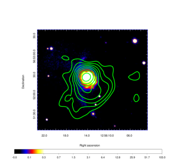
Figure 4: Left: 1.42 GHz VLA A-array total intensity contours overlaid on SDSS (Ahumada et al., 2020) $\it{g}$-band optical image in color. The color scale extends from 0 to 136.3 $\times$ 14 nJy or 0 nJy to 1.9 $\mu$Jy. Right: 1.42 GHz C-array total intensity contours overlaid on SDSS $\it{g}$-band optical image in color. The color scale extends from 0 to 103 $\times$ 14 nJy or 0 nJy to 1.4 $\mu$Jy.

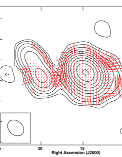
Figure 5: 1.42 GHz VLA D-array total intensity contour image with polarisation vectors in red. Contour levels are in percentage of peak surface brightness (=280.3 mJy beam^-1), with contours levels increasing in steps of 2, with the lowest contour level being $\pm 0.085$%. Polarization vector of length 1$\arcsec$ corresponds to fractional polarization of 1.6%.

Table 2: Summary of radio total intensity and polarization properties

Data	Component	Total flux	Polarized flux	Fractional	Polarization
		density ($I$, mJy)	density ($P$, mJy)	polarization ($P/I$, %)	angle ($\chi$, $\degr$)
	Core	$246\pm 23$	$4.5\pm 0.2$	$2.1\pm 0.1$	$38\pm 1$
A-array 1.4 GHz	Jet	13	$7\pm 1$	$48\pm 10$	$-7\pm 3$
	Core	$265\pm 25$	$2.5\pm 0.3$	$2.0\pm 0.3$	$-9\pm 4$
C-array 1.4 GHz	Jet+Wind	43	$7.5\pm 0.8$	$29\pm 4$	$-6\pm 4$
D-array 1.4 GHz	Core+Jet+Wind	$318\pm 28$	$22.2\pm 0.3$	$17\pm 2$	$-28\pm 3$
A-array 4.9 GHz	Core	$260\pm 24$	…	…	…
	Core	$260\pm 25$	$5.6\pm 0.3$	$2.8\pm 0.2$	$-3\pm 2$
B-array 4.9 GHz	Wind	1.8	…	…	…
	Core	$261\pm 26$	$1.0\pm 0.1$	$1.2\pm 0.2$	$24\pm 6$
C-array 4.9 GHz	Jet	12.0	$4.0\pm 0.6$	$40\pm 7$	$-19\pm 5$
	Core	$288\pm 27$	$4.6\pm 0.1$	$3.0\pm 0.4$	$-66\pm 2$
D-array 4.9 GHz	Jet+Wind	6.2	$2.7\pm 0.2$	$20\pm 3$	$-22\pm 4$

4 Discussion

We discuss now the nature of the kpc-scale radio emission in Mrk 231 and the contributions from various outflow mechanisms.

4.1 Radio Jet

The radio morphology and polarization structures of the 1.4 GHz A-array and 4.9 GHz C-array images (Figure 2) present a weakly collimated AGN jet exhibiting poloidal inferred B-fields along the spine of the jet (e.g., in III Zw 2; Silpa et al., 2021). The radio structure similar to the one revealed in our 1.4 GHz A-array image has also been detected by Morganti et al. (2016); they refer to it as the “bridge”. Moreover, the total intensity and polarization structure of the 4.9 GHz C-array image resemble the 1.4 GHz images presented in Figures 4a and 5 of Ulvestad et al. (1999a). They suggest that the diffuse lobe emission to the south is non-stellar in origin and is powered by a radio jet. They also attribute the wrapping of the B-fields around the outer edges of the lobe to jet emission. Similar B-field morphology is observed in the southern lobe of our 4.9 GHz C-array image but with an offset in the polarization angles at some places and consistent at other places, suggestive of a non-uniform Faraday screen.

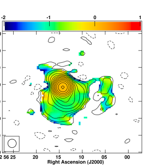
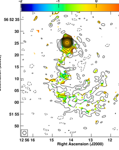
Figure 7: $1.43-4.86$ GHz spectral index images in colour with total intensity contours. Left: 15 arcsec resolution image. Contour levels are in percentage of peak surface brightness (=271.1 mJy beam^-1), with contours levels increasing in steps of 2, with the lowest contour level being $\pm 0.021$%. The color scale extends from $-$2.0 to 1.0. Right: 1.5 arcsec resolution image. Contour levels are in percentage of peak surface brightness (=232.3 mJy beam^-1), with contours levels increasing in steps of 2, with the lowest contour level being $\pm 0.021$%. The color scale extends from $-$2.0 to 1.0.

Apart from the high levels of linear polarization and well-ordered B-fields indicating non-thermal jet emission, the non-thermal nature is also confirmed by the $1.4-4.9$ GHz spectral index images presented in the left and right panels of Figure 7. The $1.4-4.9$ GHz spectral index images reveal a flat spectrum radio core ($\alpha=-0.25\pm 0.02$ for 15$\arcsec$ and $\alpha=-0.14\pm 0.04$ for 1.5$\arcsec$ resolution images), consistent with the synchrotron self-absorbed base of a relativistic jet, and a steep spectrum lobe emission to the south ($\alpha=-0.81\pm 0.09$ for 15$\arcsec$ and $\alpha=-0.5\pm 0.4$ for 1.5$\arcsec$ resolution images), consistent with optically thin synchrotron emission.

4.2 Wind

The rotating $\chi$ vectors at the core edges of Mrk 231 (Figure 1) suggest tangential or compressed B-fields, assuming optically thin emission. They could either be indicative of B-fields compressed along the edges by an expanding cocoon driven by a wind resulting from the disruption of an inclined jet (Mukherjee et al., 2018) or could represent the base of a magnetically-driven AGN wind (Palumbo et al., 2020) or a magnetized starburst-driven wind (see Section 3.4) threaded by toroidal B-fields. Moreover, the sub-kpc scale disk-like emission detected in the 1.4 GHz VLBA image of Carilli et al. (1998) (see also Morganti et al., 2016) may represent the base of the wind.

The transverse B-fields revealed in the 1.4 GHz C-array and 4.9 GHz D-array images (Figure 3) could be interpreted as arising from the ordering and amplification of B-fields by compression due to a series of transverse shocks, or could represent a toroidal component of a large-scale helical B-field associated with the jet (Gabuzda et al., 1994; Lister et al., 1998; Pushkarev et al., 2017). However, the works of Miller et al. (2012) and Mehdipour & Costantini (2019) suggest an association of toroidal B-fields with magnetically-driven AGN winds and poloidal B-fields with jets. Therefore, one cannot rule out the possibility of a magnetized accretion disk wind or the outer layers of a broadened jet (like a jet sheath; Mukherjee et al., 2018) threaded by toroidal B-fields, sampled on larger spatial scales (e.g., in III Zw 2; Silpa et al., 2021).

4.3 Jet & Wind Composite

We find that the multi-scale polarization images presented in the current work probe different layers of the kpc-scale radio emission that are sampled at different resolutions. The parallel inferred B-fields in the regions close to the core could represent a poloidal B-field component in the spine of the weakly collimated jet. The transverse inferred B-fields in the core are suggestive of a toroidal B-field component at the base of the outflow, which continues all the way up to the edge of the southern lobe. The transverse inferred B-fields in the lobe could represent B-field amplification due to shock compression by a radiatively driven AGN wind, or toroidal B-fields threading a magnetized accretion disk wind or the outer layers of a broadened jet.

Thus, our results so far point to a composite jet and “wind” outflow in Mrk 231, where the weakly collimated AGN jet with poloidal inferred B-fields is immersed inside a broader magnetized “wind” with toroidal inferred B-fields (see also Section 4.4 that discusses the idea of composite jet and wind outflow in Mrk 231, based on the energetic arguments). The “wind” may either comprise both nuclear starburst (close to the core) and AGN winds, or the outer layers of a broadened jet. Such a co-axial jet and wind outflow would appear co-spatial in projection, similar to that proposed in III Zw 2 (Silpa et al., 2021). Such a co-axial outflow comprising of jet and MHD disk wind, has also been revealed in the protostellar system HH 212 (Lee et al., 2021).

Reynolds et al. (2009) show the dereddened radio-loudness of Mrk 231 to be $1.4<\mathrm{R}<3.8$, making it a radio-quiet AGN. Interestingly, Reynolds et al. (2017) suggest that Mrk 231 is transitioning from radio-quiet to radio-loud state. In this respect as well as other properties, Mrk 231 shows close similarities to the radio-intermediate AGN III Zw 2 (Brunthaler et al., 2000; Silpa et al., 2021).

4.4 Relative contributions of Jet & Wind

In Section 3.5.1, we derive $\eta_{\mathrm{jet}}=0.012$ using the relation by Merloni & Heinz (2007). This is in agreement with other measurements of $\eta_{\mathrm{jet}}$ in the literature (for e.g., Balmaverde et al., 2008; Nemmen & Tchekhovskoy, 2015). The implications of $\eta_{\mathrm{jet}}\sim 0.01$ are: (1) about 1% of the rest mass energy of accreted matter is extracted. (2) the mechanism for the extraction might be Blandford & Znajek (1977). We note that $\eta_{\mathrm{jet}}$ derived using Willott et al. (1999) and Punsly (2005) relations is lower than that derived using the Merloni & Heinz (2007) relation by 2 orders of magnitude. This could suggest that the Willott et al. (1999) model underestimates the fraction of the accreted rest mass energy which is carried away by the jet in radio-quiet AGN like Mrk 231, given that Merloni & Heinz (2007) relation is derived for a sample of low-luminosity AGN whereas Willott et al. (1999) relation is derived for a sample of radio-powerful AGN. Moreover, it is well-known that the intrinsic flux density of a relativistic jet is Doppler-beamed in the direction towards the observer and at small viewing angles of the jet, the beamed emission appears even stronger (Cohen et al., 2007; Pearson & Zensus, 1987). Merloni & Heinz (2007) have corrected for the relativistic beaming effects in their relation. This should take care of any potential disparity in the energetic analysis presented here, that may arise due to the outflow in Mrk 231 being oriented close to the line of sight.

Interestingly, we obtain consistent values for S_SBwind using both Leitherer et al. (1999) and Dalla Vecchia & Schaye (2008) models but different values for S_AGNwind (see Sections 3.5.2 and 3.5.3). The total radio luminosity estimated (say, S_tot) is 294 mJy in 4.9 GHz D-array image, 308 mJy in the 1.4 GHz C-array image and 318 mJy in the 1.4 GHz D-array image. Therefore, our estimation suggests that the starburst-driven wind accounts for $\sim$ 8% of the total radio emission detected in the lower resolution image at 4.9 GHz and $\sim$ 20% of the total radio emission detected in the lower resolution image at 1.4 GHz in Mrk 231. Using the estimates of S_SBwind and S_AGNwind, we now estimate the contribution of the weakly collimated jet to the total radio emission in the lower resolution images. Essentially, we estimate: $\mathrm{S_{jet}=S_{tot}-(S_{SBwind}+S_{AGNwind})}$. We also note that the relative contributions of jet and wind will change with a change in the coupling efficiency.

For a coupling efficiency of 5%, the Leitherer et al. (1999) model yields S_AGNwind $\sim$ 360 mJy at 1.4 GHz and $\sim$ 130 mJy at 4.9 GHz. This gives S_jet = 294 $-$ (23+130) = 141 mJy in the 4.9 GHz D-array image. We note that the value of S_AGNwind obtained at 1.4 GHz is slightly higher than S_tot obtained in the 1.4 GHz C- and D-array images. On the other hand, the Dalla Vecchia & Schaye (2008) model yields S_AGNwind $\sim$ 1.1 Jy at 1.4 GHz and $\sim$ 400 mJy at 4.9 GHz assuming Chabrier (2003) IMF and $\sim$ 1.8 Jy at 1.4 GHz and $\sim$ 650 mJy at 4.9 GHz assuming Salpeter (1955) IMF. We note that the value of S_AGNwind obtained using Dalla Vecchia & Schaye (2008) model is higher than S_tot for all three images. This could suggest that the Dalla Vecchia & Schaye (2008) model over-estimates the AGN wind contribution and predicts negligible contributions from starburst-driven wind and radio jet for a source like Mrk 231.

For a coupling efficiency of 0.5%, the Leitherer et al. (1999) model yields S_AGNwind $\sim$ 36 mJy at 1.4 GHz and $\sim$ 13 mJy at 4.9 GHz. This gives S_jet = 294 $-$ (23+13) = 258 mJy in the 4.9 GHz D-array image, S_jet = 308 $-$ (64+36) = 208 mJy in the 1.4 GHz C-array and S_jet = 318 $-$ (64+36) = 218 mJy in the 1.4 GHz D-array image. On the other hand, the Dalla Vecchia & Schaye (2008) model yields S_AGNwind $\sim$ 110 mJy at 1.4 GHz and $\sim$ 40 mJy at 4.9 GHz assuming Chabrier (2003) IMF and S_AGNwind $\sim$ 180 mJy at 1.4 GHz and $\sim$ 65 mJy at 4.9 GHz assuming Salpeter (1955) IMF. The Chabrier (2003) IMF yields S_jet = 294 $-$ (23+40) = 231 mJy in the 4.9 GHz D-array image, S_jet = 308 $-$ (64+110) = 134 mJy in the 1.4 GHz C-array and S_jet = 318 $-$ (64+110) = 144 mJy in the 1.4 GHz D-array image. The Salpeter (1955) IMF yields S_jet = 294 $-$ (23+65) = 206 mJy in the 4.9 GHz D-array image, S_jet = 308 $-$ (64+180) = 64 mJy in the 1.4 GHz C-array and S_jet = 318 $-$ (64+180) = 74 mJy in the 1.4 GHz D-array image.

Feruglio et al. (2015) find that the energy outflow rates of the ultra-fast outflow and molecular outflow traced by CO in Mrk 231 are in agreement with the coupling efficiency required in the Di Matteo et al. (2005) AGN feedback model. Morganti et al. (2016) find that the jet power is not sufficient to drive the HI and molecular outflows in Mrk 231. These works favour a wide-angle wind origin for these gas outflows based on morphology and energetics. Rupke & Veilleux (2011) find that the mass and energy outflow rates of the neutral atomic outflow traced by Na I D in Mrk 231 are consistent with the coupling efficiency required in the Hopkins & Elvis (2010) AGN feedback model. We note that when 0.5% coupling efficiency (i.e., the Hopkins & Elvis, 2010, model) is assumed, the radio contribution of the jet estimated using Leitherer et al. (1999) model and Dalla Vecchia & Schaye (2008) model assuming Chabrier (2003) IMF, surpasses that of the wind. Overall, it thus appears that although the cold gas outflows favour a wide-angle wind origin, one cannot unambiguously rule out the presence of a low-power weakly collimated large-scale jet in Mrk 231.

Another interesting finding is that using S_jet estimated from the 4.9 GHz D-array image in equations (5)-(7), we obtain $\eta_{\mathrm{jet}}$ of $\sim$0.007 with 5% coupling efficiency and $\sim$0.011 with 0.5% coupling efficiency. Thus, $\eta_{\mathrm{jet}}$ estimated using higher and lower resolution images are broadly consistent with each other. Overall, the coupling efficiency can have a range of values without changing the overall picture in Mrk 231. We find a broad agreement between the energetics of the radio outflows derived using the approach discussed in Section 3.5, and the energetics of the neutral atomic and molecular outflows reported in the literature, suggesting that our approach is valid and close to reality.

4.5 Curvature of the kpc-scale jet

The curved kpc-scale weakly collimated jet in Mrk 231 could arise either from an interaction between the jet and the surrounding medium or from a precessing jet. Jet precession could result from a warped accretion disk or a binary black hole (Pringle, 1996; Caproni & Abraham, 2004; Krause et al., 2019) or a precessing accretion disk owing to disc instabilities from an ongoing merger event (Liska et al., 2018). The disturbed morphology of the host galaxy and the presence of tidal tails suggest that Mrk 231 is probably at the final stage of a merger (Armus et al., 1994; Lipari et al., 1994).

A binary black hole has been proposed in Mrk 231 by Yan et al. (2015), in order to explain the unusual optical-UV spectrum observed in this source. They suggest that while the smaller-mass black hole ($4.5\times 10^{6}$ M_☉) accretes as a thin accretion disk and the larger-mass black hole ($1.5\times 10^{8}$ M_☉) accretes via radiatively inefficiently advection dominated accretion flow (ADAF), the two black holes are also surrounded by a circumbinary disk. However, the binary black hole scenario has come under scrutiny by recent infrared and ultraviolet spectral studies of Mrk 231 (e.g., Veilleux et al., 2016; Leighly et al., 2016). Hence, there is presently no strong observational evidence in favor of the binary black hole in Mrk 231.

4.6 Matter-dominated outflow

A “failed” jet scenario has been proposed in Mrk 231 (Rupke & Veilleux, 2011; Morganti et al., 2016; Reynolds et al., 2020). Wang et al. (2021) argue that the jet in Mrk 231 is obstructed by the dense ISM within a few tens pc scales, which prevents its growth to larger scales. A low ionization BAL wind (Lipari et al., 1994; Smith et al., 1995), a high ionization X-ray absorbing wind (Feruglio et al., 2015; Reynolds et al., 2017) and huge amounts of circumnuclear dust (Smith et al., 1995), all contribute towards a dense nuclear environment that may slow down or disrupt the jet.

Sub-relativistic expansion of the pc-scale jet in Mrk 231 (Ulvestad et al., 1999b) is similar to the ‘slow’ phase seen in III Zw 2 (Brunthaler et al., 2000). This suggests that the region of relativistic expansion in Mrk 231 is on even smaller spatial scales, or that the expansion is intrinsically slow quite early on. The multi-scale radio morphology and spectral index values (Section 3.1), polarization structures (Section 3.2) and energetic arguments (Sections 3.5 and 4.4) are consistent with the presence of a kpc-scale weakly collimated jet in Mrk 231. Therefore, it is possible that the jet in Mrk 231 was launched relativistically but slowed down without getting completely disrupted.

As discussed in Section 3.3, we conclude that for both poloidal inferred B-fields associated with the spine of the weakly collimated jet and toroidal inferred B-fields associated with the wind/jet sheath, $\beta$ increases with increasing distance from the core, implying that the composite jet and wind outflow in Mrk 231 becomes increasingly matter-dominated away from the core (e.g., Meier, 2003). Simulations by Mukherjee et al. (2020) suggest that the matter-dominated and low-power jets are more susceptible to instabilities than the Poynting flux dominated jets, and therefore could get easily deaccelerated/decollimated but not terminated, such as that seen in Mrk 231.

5 Summary and Conclusions

Our multi-frequency, multi-scale polarization-sensitive VLA observations of the Seyfert 1 galaxy and BALQSO, Mrk 231 at 1.4 and 4.9 GHz reveal the likely presence of multiple radio components with characteristic B-field geometries. We summarise our primary findings below.

1. Mrk 231 shows a core-dominated radio source with extended emission in total intensity on kpc-scales with the VLA. A combination of a weakly collimated jet and a wind or jet sheath, oriented at a small angle to line of sight, can explain the observed total intensity and polarization structures.

2. The “wind” component of the composite outflow may be driven by both a starburst (close to the core) and the AGN, where the latter maybe the primary driver. Moving away from the core, the “wind” component may also comprise the outer layers (or sheath) of a weakly collimated jet.

3. The model of a kpc-scale weakly collimated jet/lobe in Mrk 231 is strengthened by its C-shaped morphology, steep spectral index throughout, complexities in the B-field structures, and the presence of self-similar structures observed on the 10-parsec-scale in the literature. The latter may even suggest the presence of episodic jet activity in Mrk 231.

4. Our results suggest that the starburst-driven wind accounts for $\sim$ 8% of the total radio emission detected in the lower resolution image at 4.9 GHz and $\sim$ 20% of the total radio emission detected in the lower resolution image at 1.4 GHz in Mrk 231.

5. The inferred value of the (weakly collimated) jet production efficiency, $\eta_{\mathrm{jet}}\sim 0.01$ using the relation by Merloni & Heinz (2007), is consistent with other estimates in the literature and its implications are: (1) about 1% of the rest mass energy of accreted matter is extracted. (2) the mechanism for the extraction might be Blandford & Znajek (1977).

6. Overall, we conclude that kpc-scale weakly collimated radio jet in Mrk 231 with poloidal inferred B-fields is curved and one-sided, and immersed inside a broader magnetized wind with toroidal inferred B-fields, with the composite outflow being matter-dominated.

Data Availability

The data underlying this article will be shared on reasonable request to the corresponding author. The VLA data underlying this article can be obtained from the NRAO Science Data Archive (https://archive.nrao.edu/archive/advquery.jsp) using the proposal id: AB740.

References

- Ahumada et al. (2020) Ahumada R., et al., 2020, ApJS, 249, 3
- Antonucci (1993) Antonucci R., 1993, ARA&A, 31, 473
- Armus et al. (1994) Armus L., Surace J. A., Soifer B. T., Matthews K., Graham J. R., Larkin J. E., 1994, AJ, 108, 76
- Baan (1985) Baan W. A., 1985, Nature, 315, 26
- Balmaverde et al. (2008) Balmaverde B., Baldi R. D., Capetti A., 2008, A&A, 486, 119
- Baum & Heckman (1989) Baum S. A., Heckman T., 1989, ApJ, 336, 702
- Baum et al. (1993) Baum S. A., O’Dea C. P., Dallacassa D., de Bruyn A. G., Pedlar A., 1993, ApJ, 419, 553
- Begelman et al. (1984) Begelman M. C., Blandford R. D., Rees M. J., 1984, Reviews of Modern Physics, 56, 255
- Bell (2003) Bell E. F., 2003, ApJ, 586, 794
- Blandford & Znajek (1977) Blandford R. D., Znajek R. L., 1977, MNRAS, 179, 433
- Boksenberg et al. (1977) Boksenberg A., Carswell R. F., Allen D. A., Fosbury R. A. E., Penston M. V., Sargent W. L. W., 1977, MNRAS, 178, 451
- Bondi et al. (2001) Bondi M., Parma P., de Ruiter H., Fanti R., Laing R. A., 2001, in Laing R. A., Blundell K. M., eds, Astronomical Society of the Pacific Conference Series Vol. 250, Particles and Fields in Radio Galaxies Conference. p. 276
- Brunthaler et al. (2000) Brunthaler A., et al., 2000, A&A, 357, L45
- Burn (1966) Burn B. J., 1966, MNRAS, 133, 67
- Caproni & Abraham (2004) Caproni A., Abraham Z., 2004, ApJ, 602, 625
- Carilli et al. (1998) Carilli C. L., Wrobel J. M., Ulvestad J. S., 1998, AJ, 115, 928
- Chabrier (2003) Chabrier G., 2003, PASP, 115, 763
- Cohen et al. (2007) Cohen M. H., Lister M. L., Homan D. C., Kadler M., Kellermann K. I., Kovalev Y. Y., Vermeulen R. C., 2007, ApJ, 658, 232
- Colbert et al. (1996) Colbert E. J. M., Baum S. A., Gallimore J. F., O’Dea C. P., Christensen J. A., 1996, ApJ, 467, 551
- Condon et al. (1991) Condon J. J., Frayer D. T., Broderick J. J., 1991, AJ, 101, 362
- Condon et al. (2002) Condon J. J., Cotton W. D., Broderick J. J., 2002, AJ, 124, 675
- Dalla Vecchia & Schaye (2008) Dalla Vecchia C., Schaye J., 2008, MNRAS, 387, 1431
- Di Matteo et al. (2005) Di Matteo T., Springel V., Hernquist L., 2005, Nature, 433, 604
- Feruglio et al. (2015) Feruglio C., et al., 2015, A&A, 583, A99
- Gabuzda et al. (1994) Gabuzda D. C., Mullan C. M., Cawthorne T. V., Wardle J. F. C., Roberts D. H., 1994, ApJ, 435, 140
- Gallagher et al. (2002) Gallagher S. C., Brandt W. N., Chartas G., Garmire G. P., Sambruna R. M., 2002, ApJ, 569, 655
- Ho & Peng (2001) Ho L. C., Peng C. Y., 2001, ApJ, 555, 650
- Hopkins & Elvis (2010) Hopkins P. F., Elvis M., 2010, MNRAS, 401, 7
- Hota & Saikia (2006) Hota A., Saikia D. J., 2006, MNRAS, 371, 945
- Kellermann et al. (1989) Kellermann K. I., Sramek R., Schmidt M., Shaffer D. B., Green R., 1989, AJ, 98, 1195
- Kharb et al. (2006) Kharb P., O’Dea C. P., Baum S. A., Colbert E. J. M., Xu C., 2006, ApJ, 652, 177
- Kharb et al. (2010) Kharb P., Hota A., Croston J. H., Hardcastle M. J., O’Dea C. P., Kraft R. P., Axon D. J., Robinson A., 2010, ApJ, 723, 580
- Kharb et al. (2012) Kharb P., O’Dea C. P., Tilak A., Baum S. A., Haynes E., Noel-Storr J., Fallon C., Christiansen K., 2012, ApJ, 754, 1
- Krause et al. (2019) Krause M. G. H., et al., 2019, MNRAS, 482, 240
- Laing & Bridle (2002) Laing R. A., Bridle A. H., 2002, MNRAS, 336, 1161
- Lee et al. (2021) Lee C.-F., Tabone B., Cabrit S., Codella C., Podio L., Ferreira J., Jacquemin-Ide J., 2021, ApJ, 907, L41
- Leighly et al. (2016) Leighly K. M., Terndrup D. M., Gallagher S. C., Lucy A. B., 2016, ApJ, 829, 4
- Leitherer et al. (1999) Leitherer C., et al., 1999, ApJS, 123, 3
- Lipari et al. (1994) Lipari S., Colina L., Macchetto F., 1994, ApJ, 427, 174
- Liska et al. (2018) Liska M., Hesp C., Tchekhovskoy A., Ingram A., van der Klis M., Markoff S., 2018, MNRAS, 474, L81
- Lister et al. (1998) Lister M. L., Marscher A. P., Gear W. K., 1998, ApJ, 504, 702
- Livio et al. (1999) Livio M., Ogilvie G. I., Pringle J. E., 1999, ApJ, 512, 100
- McCutcheon & Gregory (1978) McCutcheon W. H., Gregory P. C., 1978, AJ, 83, 566
- Mehdipour & Costantini (2019) Mehdipour M., Costantini E., 2019, A&A, 625, A25
- Meier (2003) Meier D. L., 2003, New Astron. Rev., 47, 667
- Merloni & Heinz (2007) Merloni A., Heinz S., 2007, MNRAS, 381, 589
- Miller et al. (2012) Miller J. M., et al., 2012, ApJ, 759, L6
- Morganti et al. (2016) Morganti R., Veilleux S., Oosterloo T., Teng S. H., Rupke D., 2016, A&A, 593, A30
- Mukherjee et al. (2018) Mukherjee D., Bicknell G. V., Wagner A. Y., Sutherland R. S., Silk J., 2018, MNRAS, arXiv 1803.08305,
- Mukherjee et al. (2020) Mukherjee D., Bodo G., Mignone A., Rossi P., Vaidya B., 2020, MNRAS, 499, 681
- Neff & Ulvestad (1988) Neff S. G., Ulvestad J. S., 1988, AJ, 96, 841
- Nemmen & Tchekhovskoy (2015) Nemmen R. S., Tchekhovskoy A., 2015, MNRAS, 449, 316
- Nesvadba et al. (2017) Nesvadba N. P. H., Drouart G., De Breuck C., Best P., Seymour N., Vernet J., 2017, A&A, 600, A121
- Novikov & Thorne (1973) Novikov I. D., Thorne K. S., 1973, in Black Holes (Les Astres Occlus). pp 343–450
- O’Dea & Owen (1987) O’Dea C. P., Owen F. N., 1987, ApJ, 316, 95
- Palumbo et al. (2020) Palumbo D. C. M., Wong G. N., Prather B. S., 2020, ApJ, 894, 156
- Panessa et al. (2019) Panessa F., Baldi R. D., Laor A., Padovani P., Behar E., McHardy I., 2019, Nature Astronomy, 3, 387
- Park et al. (2019) Park J., Hada K., Kino M., Nakamura M., Ro H., Trippe S., 2019, ApJ, 871, 257
- Pearson & Zensus (1987) Pearson T. J., Zensus J. A., 1987, in Zensus J. A., Pearson T. J., eds, Superluminal Radio Sources. pp 1–11
- Peterson (1997) Peterson B. M., 1997, An Introduction to Active Galactic Nuclei
- Pringle (1996) Pringle J. E., 1996, MNRAS, 281, 357
- Punsly (2005) Punsly B., 2005, ApJ, 623, L9
- Pushkarev et al. (2017) Pushkarev A., Kovalev Y., Lister M., Savolainen T., Aller M., Aller H., Hodge M., 2017, Galaxies, 5, 93
- Rawlings & Saunders (1991) Rawlings S., Saunders R., 1991, Nature, 349, 138
- Reynolds et al. (2009) Reynolds C., Punsly B., Kharb P., O’Dea C. P., Wrobel J., 2009, ApJ, 706, 851
- Reynolds et al. (2017) Reynolds C., Punsly B., Miniutti G., O’Dea C. P., Hurley-Walker N., 2017, ApJ, 836, 155
- Reynolds et al. (2020) Reynolds C., Punsly B., Miniutti G., O’Dea C. P., Hurley-Walker N., 2020, ApJ, 891, 59
- Rupke & Veilleux (2011) Rupke D. S. N., Veilleux S., 2011, ApJ, 729, L27
- Rupke & Veilleux (2013) Rupke D. S. N., Veilleux S., 2013, ApJ, 768, 75
- Rupke et al. (2017) Rupke D. S. N., Gültekin K., Veilleux S., 2017, ApJ, 850, 40
- Salpeter (1955) Salpeter E. E., 1955, ApJ, 121, 161
- Sanders et al. (1988a) Sanders D. B., Soifer B. T., Elias J. H., Madore B. F., Matthews K., Neugebauer G., Scoville N. Z., 1988a, ApJ, 325, 74
- Sanders et al. (1988b) Sanders D. B., Soifer B. T., Elias J. H., Neugebauer G., Matthews K., 1988b, ApJ, 328, L35
- Sebastian et al. (2019a) Sebastian B., Kharb P., O’Dea C. P., Gallimore J. F., Baum S. A., 2019a, MNRAS, 490, L26
- Sebastian et al. (2019b) Sebastian B., Kharb P., O’Dea C. P., Colbert E. J. M., Baum S. A., 2019b, ApJ, 883, 189
- Sebastian et al. (2020) Sebastian B., Kharb P., O’Dea C. P., Gallimore J. F., Baum S. A., 2020, MNRAS, 499, 334
- Shankar et al. (2008) Shankar F., Cavaliere A., Cirasuolo M., Maraschi L., 2008, ApJ, 676, 131
- Sharma et al. (2014) Sharma P., Roy A., Nath B. B., Shchekinov Y., 2014, MNRAS, 443, 3463
- Silpa et al. (2021) Silpa S., Kharb P., Harrison C. M., Ho L. C., Jarvis M. E., Ishwara-Chandra C. H., Sebastian B., 2021, MNRAS submitted
- Smith et al. (1995) Smith P. S., Schmidt G. D., Allen R. G., Angel J. R. P., 1995, ApJ, 444, 146
- Strickland & Heckman (2009) Strickland D. K., Heckman T. M., 2009, ApJ, 697, 2030
- Surace et al. (1998) Surace J. A., Sanders D. B., Vacca W. D., Veilleux S., Mazzarella J. M., 1998, ApJ, 492, 116
- Thornton et al. (1998) Thornton K., Gaudlitz M., Janka H. T., Steinmetz M., 1998, ApJ, 500, 95
- Ulvestad et al. (1981) Ulvestad J. S., Wilson A. S., Sramek R. A., 1981, ApJ, 247, 419
- Ulvestad et al. (1999a) Ulvestad J. S., Wrobel J. M., Carilli C. L., 1999a, ApJ, 516, 127
- Ulvestad et al. (1999b) Ulvestad J. S., Wrobel J. M., Roy A. L., Wilson A. S., Falcke H., Krichbaum T. P., 1999b, ApJ, 517, L81
- Veilleux et al. (2005) Veilleux S., Cecil G., Bland-Hawthorn J., 2005, ARA&A, 43, 769
- Veilleux et al. (2009) Veilleux S., et al., 2009, ApJS, 182, 628
- Veilleux et al. (2016) Veilleux S., Meléndez M., Tripp T. M., Hamann F., Rupke D. S. N., 2016, ApJ, 825, 42
- Wang et al. (2021) Wang A., An T., Jaiswal S., Mohan P., Wang Y., Baan W. A., Zhang Y., Yang X., 2021, arXiv e-prints, p. arXiv:2102.12644
- Willott et al. (1999) Willott C. J., Rawlings S., Blundell K. M., Lacy M., 1999, MNRAS, 309, 1017
- Yan et al. (2015) Yan C.-S., Lu Y., Dai X., Yu Q., 2015, ApJ, 809, 117
- Zakamska & Greene (2014) Zakamska N. L., Greene J. E., 2014, MNRAS, 442, 784