CANITA: Faster Rates for Distributed Convex Optimization with Communication Compression

Abstract

Due to the high communication cost in distributed and federated learning, methods relying on compressed communication are becoming increasingly popular. Besides, the best theoretically and practically performing gradient-type methods invariably rely on some form of acceleration/momentum to reduce the number of communications (faster convergence), e.g., Nesterov’s accelerated gradient descent [31, 32] and Adam [14]. In order to combine the benefits of communication compression and convergence acceleration, we propose a compressed and accelerated gradient method based on ANITA [20] for distributed optimization, which we call CANITA. Our CANITA achieves the first accelerated rate $O\bigg{(}\sqrt{\Big{(}1+\sqrt{\frac{\omega^{3}}{n}}\Big{)}\frac{L}{\epsilon}}+\omega\big{(}\frac{1}{\epsilon}\big{)}^{\frac{1}{3}}\bigg{)}$, which improves upon the state-of-the-art non-accelerated rate $O\left((1+\frac{\omega}{n})\frac{L}{\epsilon}+\frac{\omega^{2}+\omega}{\omega+n}\frac{1}{\epsilon}\right)$ of DIANA [12] for distributed general convex problems, where $\epsilon$ is the target error, $L$ is the smooth parameter of the objective, $n$ is the number of machines/devices, and $\omega$ is the compression parameter (larger $\omega$ means more compression can be applied, and no compression implies $\omega=0$). Our results show that as long as the number of devices $n$ is large (often true in distributed/federated learning), or the compression $\omega$ is not very high, CANITA achieves the faster convergence rate $O\Big{(}\sqrt{\frac{L}{\epsilon}}\Big{)}$, i.e., the number of communication rounds is $O\Big{(}\sqrt{\frac{L}{\epsilon}}\Big{)}$ (vs. $O\big{(}\frac{L}{\epsilon}\big{)}$ achieved by previous works). As a result, CANITA enjoys the advantages of both compression (compressed communication in each round) and acceleration (much fewer communication rounds).

1 Introduction

With the proliferation of edge devices, such as mobile phones, wearables and smart home appliances, comes an increase in the amount of data rich in potential information which can be mined for the benefit of humankind. One of the approaches of turning the raw data into information is via federated learning [15, 29], where typically a single global supervised model is trained in a massively distributed manner over a network of heterogeneous devices.

Training supervised distributed/federated learning models is typically performed by solving an optimization problem of the form

$$\vspace{-1.8mm}\min_{x\in{\mathbb{R}}^{d}}\Big{\{}f(x):=\frac{1}{n}\sum\limits_{i=1}^{n}f_{i}(x)\Big{\}},$$ (1)

where $n$ denotes the number of devices/machines/workers/clients, and $f_{i}:{\mathbb{R}}^{d}\rightarrow{\mathbb{R}}$ is a loss function associated with the data stored on device $i$. We will write

$$x^{*}:=\arg\min_{x\in{\mathbb{R}}^{d}}f(x).$$

If more than one minimizer exist, $x^{*}$ denotes an arbitrary but fixed solution. We will rely on the solution concept captured in the following definition:

Definition 1

A random vector $\widehat{x}\in{\mathbb{R}}^{d}$ is called an $\epsilon$-solution of the distributed problem (1) if

$${\mathbb{E}}\left[f(\widehat{x})\right]-f(x^{*})\leq\epsilon,$$

where the expectation is with respect to the randomness inherent in the algorithm used to produce $\widehat{x}$.

In distributed and federated learning problems of the form (1), communication of messages across the network typically forms the key bottleneck of the training system. In the modern practice of supervised learning in general and deep learning in particular, this is exacerbated by the reliance on massive models described by millions or even billions of parameters. For these reasons, it is very important to devise novel and more efficient training algorithms capable of decreasing the overall communication cost, which can be formalized as the product of the number of communication rounds necessary to train a model of sufficient quality, and the computation and communication cost associated with a typical communication round.

1.1 Methods with compressed communication

One of the most common strategies for improving communication complexity is communication compression [37, 1, 40, 8, 30, 9, 26, 24]. This strategy is based on the reduction of the size of communicated messages via the application of a suitably chosen lossy compression mechanism, saving precious time spent in each communication round, and hoping that this will not increase the total number of communication rounds.

Several recent theoretical results suggest that by combining an appropriate (randomized) compression operator with a suitably designed gradient-type method, one can obtain improvement in the total communication complexity over comparable baselines not performing any compression. For instance, this is the case for distributed compressed gradient descent (CGD) [1, 13, 8, 24], and distributed CGD methods which employ variance reduction to tame the variance introduced by compression [7, 30, 9, 24, 6].

1.2 Methods with acceleration

The acceleration/momentum of gradient-type methods is widely-studied in standard optimization problems, which aims to achieve faster convergence rates (fewer communication rounds) [33, 31, 32, 17, 28, 2, 18, 16, 23, 20]. Deep learning practitioners typically rely on Adam [14], or one of its many variants, which besides other tricks also adopts momentum. In particular, ANITA [20] obtains the current state-of-the-art convergence results for convex optimization. In this paper, we will adopt the acceleration from ANITA [20] to the distributed setting with compression.

1.3 Can communication compression and acceleration be combined?

Encouraged by the recent theoretical success of communication compression, and the widespread success of accelerated methods, in this paper we seek to further enhance CGD methods with acceleration/momentum, with the aim to obtain provable improvements in overall communication complexity.

Can distributed gradient-type methods theoretically benefit from the combination of gradient compression and acceleration/momentum? To the best of our knowledge, no such results exist in the general convex regime, and in this paper we close this gap by designing a method that can provably enjoy the advantages of both compression (compressed communication in each round) and acceleration (much fewer communication rounds).

While there is abundance of research studying communication compression and acceleration in isolation, there is very limited work on the combination of both approaches. The first successful combination of gradient compression and acceleration/momentum was recently achieved by the ADIANA method of Li et al. [26]. However, Li et al. [26] only provide theoretical results for strongly convex problems, and their method is not applicable to (general) convex problems. So, one needs to both design a new method to handle the convex case, and perform its analysis. A-priori, it is not clear at all what approach would work.

To the best of our knowledge, besides the initial work [26], we are only aware of two other works for addressing this question [41, 34]. However, both these works still only focus on the simpler and less practically relevant strongly convex setting. Thus, this line of research is still largely unexplored. For instance, the well-known logistic regression problem is convex but not strongly convex. Finally, even if a problem is strongly convex, the modulus of strong convexity is typically not known, or hard to estimate properly.

Table 1: Convergence rates for finding an $\epsilon$-solution ${\mathbb{E}}[f(x^{T})]-f(x^{*})\leq\epsilon$ of distributed problem (1)

Algorithms	Strongly convex	General convex	Remark
QSGD [1]	—	$O\left(\frac{L}{\epsilon}+\frac{\omega G^{2}}{n}\frac{1}{\epsilon^{2}}\right)$	✓compression $\times$ acceleration
DIANA [30]	$O\left(\Big{(}\big{(}1+\frac{\omega}{n}\big{)}\kappa+\omega\Big{)}\log\frac{1}{\epsilon}\right)$	—	✓compression $\times$ acceleration
DIANA [9]	$O\left(\Big{(}\big{(}1+\frac{\omega}{n}\big{)}\kappa+\omega\Big{)}\log\frac{1}{\epsilon}\right)$	$O\left(\big{(}1+\frac{\omega}{n}\big{)}\frac{L}{\epsilon}+\frac{\omega}{\epsilon}\right)$	✓compression $\times$ acceleration
DIANA [12]	—	$O\left(\big{(}1+\frac{\omega}{n}\big{)}\frac{L}{\epsilon}+\frac{\omega^{2}+\omega}{\omega+n}\frac{1}{\epsilon}\right)$	✓compression $\times$ acceleration
ADIANA [26]	$O$$\left(\Big{(}\sqrt{\kappa}+\sqrt{\big{(}\frac{\omega}{n}+\sqrt{\frac{\omega}{n}}\big{)}\omega\kappa}+\omega\Big{)}\log\frac{1}{\epsilon}\right)$	—	✓compression ✓acceleration
CANITA (this paper)	—	$O$$\left(\sqrt{\Big{(}1+\sqrt{\frac{\omega^{3}}{n}}\Big{)}\frac{L}{\epsilon}}+\omega\big{(}\frac{1}{\epsilon}\big{)}^{\frac{1}{3}}\right)$	✓compression ✓acceleration

2 Summary of Contributions

In this paper we propose and analyze an accelerated gradient method with compressed communication, which we call CANITA (described in Algorithm 1), for solving distributed general convex optimization problems of the form (1). In particular, CANITA can loosely be seen as a combination of the accelerated gradient method ANITA of [20], and the variance-reduced compressed gradient method DIANA of [30]. Ours is the first work provably combining the benefits of communication compression and acceleration in the general convex regime.

2.1 First accelerated rate for compressed gradient methods in the convex regime

For general convex problems, CANITA is the first compressed communication gradient method with an accelerated rate. In particular, our CANITA solves the distributed problem (1) in

$$O\left(\sqrt{\bigg{(}1+\sqrt{\tfrac{\omega^{3}}{n}}\bigg{)}\tfrac{L}{\epsilon}}+\omega\left(\tfrac{1}{\epsilon}\right)^{\frac{1}{3}}\right)$$

communication rounds, which improves upon the current state-of-the-art result

$$O\left(\left(1+\tfrac{\omega}{n}\right)\tfrac{L}{\epsilon}+\tfrac{\omega^{2}+n}{\omega+n}\tfrac{1}{\epsilon}\right)$$

achieved by the DIANA method [12]. See Table 1 for more comparisons.

Let us now illustrate the improvements coming from this new bound on an example with concrete numerical values. Let the compression ratio be $10\%$ (the size of compressed message is $0.1\cdot d$, where $d$ is the size of the uncompressed message). If random sparsification or quantization is used to achieve this, then $\omega\approx 10$ (see Section 3.1). Further, if the number of devices/machines is $n=10^{6}$, and the target error tolerance is $\epsilon=10^{-6}$, then the number of communication rounds of our CANITA method is $O(10^{3})$, while the number of communication rounds of the previous state-of-the-art method DIANA [12] is $O(10^{6})$, i.e., $O\big{(}\sqrt{\frac{L}{\epsilon}}\big{)}$ vs.  $O(\frac{L}{\epsilon})$. This is an improvement of three orders of magnitude.

Moreover, the numerical experiments in Section 6 indeed show that the performance of our CANITA is much better than previous non-accelerated compressed methods (QSGD and DIANA), corroborating the theoretical results (see Table 1) and confirming the practical superiority of our accelerated CANITA method.

2.2 Accelerated rate with limited compression for free

For strongly convex problems, Li et al. [26] showed that if the number of devices/machines $n$ is large, or the compression variance parameter $\omega$ is not very high ($\omega\leq n^{1/3}$), then their ADIANA method enjoys the benefits of both compression and acceleration (i.e., $\sqrt{\kappa}\log\frac{1}{\epsilon}$ of ADIANA vs.  $\kappa\log\frac{1}{\epsilon}$ of previous works).

In this paper, we consider the general convex setting and show that the proposed CANITA also enjoys the benefits of both compression and acceleration. Similarly, if $\omega\leq n^{1/3}$ (i.e., many devices, or limited compression variance), CANITA achieves the accelerated rate $\sqrt{\frac{L}{\epsilon}}$ vs.  $\frac{L}{\epsilon}$ of previous works. This means that the compression does not hurt the accelerated rate at all. Note that the second term $\big{(}\frac{1}{\epsilon}\big{)}^{\frac{1}{3}}$ is of a lower order compared with the first term $\sqrt{\frac{L}{\epsilon}}$.

2.3 Novel proof technique

The proof behind the analysis of CANITA is significantly different from that of ADIANA [26], which critically relies on strong convexity. Moreover, the theoretical rate in the strongly convex case is linear $O(\log\frac{1}{\epsilon})$, while it is sublinear $O(\frac{1}{\epsilon})$ or $O\big{(}\sqrt{\frac{1}{\epsilon}}\big{)}$ (accelerated) in the general convex case. We hope that our novel analysis can provide new insights and shed light on future work.

3 Preliminaries

Let $[n]$ denote the set $\{1,2,\cdots,n\}$ and $\|\cdot\|$ denote the Euclidean norm for a vector and the spectral norm for a matrix. Let $\langle u,v\rangle$ denote the standard Euclidean inner product of two vectors $u$ and $v$. We use $O(\cdot)$ and $\Omega(\cdot)$ to hide the absolute constants.

3.1 Assumptions about the compression operators

We now introduce the notion of a randomized compression operator which we use to compress the gradients to save on communication. We rely on a standard class of unbiased compressors (see Definition 2) that was used in the context of distributed gradient methods before [1, 13, 9, 24, 26].

Definition 2 (Compression operator)

A randomized map ${\mathcal{C}}:{\mathbb{R}}^{d}\mapsto{\mathbb{R}}^{d}$ is an $\omega$-compression operator if

$${\mathbb{E}}\left[{\mathcal{C}}(x)\right]=x,\qquad{\mathbb{E}}\left[\|{\mathcal{C}}(x)-x\|^{2}\right]\leq\omega\|x\|^{2},\qquad\forall x\in{\mathbb{R}}^{d}.$$ (2)

In particular, no compression (${\mathcal{C}}(x)\equiv x$) implies $\omega=0$.

It is well known that the conditions (2) are satisfied by many practically useful compression operators (see Table 1 in [3, 36]). For illustration purposes, we now present a couple canonical examples: sparsification and quantization.

Example 1 (Random sparsification).

Given $x\in{\mathbb{R}}^{d}$, the random-$k$ sparsification operator is defined by

$${\mathcal{C}}(x):=\frac{d}{k}\cdot(\xi_{k}\odot x),$$

where $\odot$ denotes the Hadamard (element-wise) product and $\xi_{k}\in\{0,1\}^{d}$ is a uniformly random binary vector with $k$ nonzero entries ($\|\xi_{k}\|_{0}=k$). This random-$k$ sparsification operator ${\mathcal{C}}$ satisfies (2) with $\omega=\frac{d}{k}-1$. By setting $k=d$, this reduces to the identity compressor, whose variance is obviously zero: $\omega=0$.

Example 2 (Random quantization).

Given $x\in{\mathbb{R}}^{d}$, the ($p,s$)-quantization operator is defined by

$${\mathcal{C}}(x):=\text{sign}(x)\cdot\|x\|_{p}\cdot\frac{1}{s}\cdot\xi_{s},$$

where $p,s\geq 1$ are integers, and $\xi_{s}\in{\mathbb{R}}^{d}$ is a random vector with $i$-th element

$$\xi_{s}(i):=\begin{cases}l+1,&\text{with probability }\frac{|x_{i}|}{\|x\|_{p}}s-l,\\ l,&\text{otherwise.}\end{cases}$$

The level $l$ satisfies $\frac{|x_{i}|}{\|x\|_{p}}\in[\frac{l}{s},\frac{l+1}{s}]$. The probability is chosen so that ${\mathbb{E}}\left[\xi_{s}(i)\right]=\frac{|x_{i}|}{\|x\|_{p}}s$. This ($p,s$)-quantization operator ${\mathcal{C}}$ satisfies (2) with $\omega=2+\frac{d^{1/p}+d^{1/2}}{s}$. In particular, QSGD [1] used $p=2$ (i.e., ($2,s$)-quantization) and proved that the expected sparsity of ${\cal C}(x)$ is ${\mathbb{E}}\left[\|{\mathcal{C}}(x)\|_{0}\right]=O\big{(}s(s+\sqrt{d})\big{)}$.

3.2 Assumptions about the functions

Throughout the paper, we assume that the functions $f_{i}$ are convex and have Lipschitz continuous gradient.

Assumption 1

Functions $f_{i}:{\mathbb{R}}^{d}\to{\mathbb{R}}$ are convex, differentiable, and $L$-smooth. The last condition means that there exists a constant $L>0$ such that for all $i\in[n]$ we have

$$\|\nabla f_{i}(x)-\nabla f_{i}(y)\|\leq L\|x-y\|,\qquad\forall x,y\in{\mathbb{R}}^{d}.$$ (3)

It is easy to see that the objective $f(x)=\frac{1}{n}\sum_{i=1}^{n}{f_{i}(x)}$ in (1) satisfies (3) provided that the constituent functions $\{f_{i}\}$ do.

4 The CANITA Algorithm

Algorithm 1 Distributed compressed accelerated ANITA method (CANITA)

0:  initial point $x^{0}\in{\mathbb{R}}^{d}$, initial shift vectors $h_{1}^{0},\dots,h_{n}^{0}\in{\mathbb{R}}^{d}$, probabilities $\{p_{t}\}$, and positive stepsizes $\{\alpha_{t}\},\{\eta_{t}\},\{\theta_{t}\}$

1:  Initialize: $w^{0}=z^{0}=x^{0}$ and $h^{0}=\frac{1}{n}\sum_{i=1}^{n}h_{i}^{0}$

2:  for $t=0,1,2,\ldots$ do

3:     $y^{t}=\theta_{t}x^{t}+(1-\theta_{t})w^{t}$

4:     for all machines $i=1,2,\ldots,n$ do in parallel

5:      Compress the shifted local gradient ${\cal C}_{i}^{t}(\nabla f_{i}(y^{t})-h_{i}^{t})$ and send the result to the server

6:      Update the local shift $h_{i}^{t+1}=h_{i}^{t}+\alpha_{t}{\cal C}_{i}^{t}(\nabla f_{i}(w^{t})-h_{i}^{t})$

7:     end for

8:     Aggregate received compressed local gradient information:  $g^{t}=h^{t}+\frac{1}{n}\sum\limits_{i=1}^{n}{\cal C}_{i}^{t}(\nabla f_{i}(y^{t})-h_{i}^{t})$ $\bullet$ Compute gradient estimator   $h^{t+1}=h^{t}+\alpha_{t}\frac{1}{n}\sum\limits_{i=1}^{n}{\cal C}_{i}^{t}(\nabla f_{i}(w^{t})-h_{i}^{t})$ $\bullet$ Maintain the average of local shifts

9:     Perform update step:  $x^{t+1}=x^{t}-\frac{\eta_{t}}{\theta_{t}}g^{t}$

10:     $z^{t+1}=\theta_{t}x^{t+1}+(1-\theta_{t})w^{t}$

11:     $w^{t+1}=\begin{cases}z^{t+1},&\text{with probability }p_{t}\\ w^{t},&\text{with probability }1-p_{t}\end{cases}$

12:  end for

In this section, we describe our method, for which we coin the name CANITA, designed for solving problem (1), which is of importance in distributed and federated learning, and contrast it to the most closely related methods ANITA [20], DIANA [30] and ADIANA [26].

4.1 CANITA: description of the method

Our proposed method CANITA, formally described in Algorithm 1, is an accelerated gradient method supporting compressed communication. It is the first method combing the benefits of acceleration and compression in the general convex regime (without strong convexity).

In each round $t$, each machine computes its local gradient (e.g., $\nabla f_{i}(y^{t})$) and then a shifted version is compressed and sent to the server (See Line 5 of Algorithm 1). The local shifts $h_{i}^{t}$ are adaptively changing throughout the iterative process (Line 6), and have the role of reducing the variance introduced by compression ${\cal C}(\cdot)$. If no compression is used, we may simply set the shifts to be $h_{i}^{t}=0$ for all $i,t$. The server subsequently aggregates all received messages to obtain the gradient estimator $g^{t}$ and maintain the average of local shifts $h^{t+1}$ (Line 8), and then perform gradient update step (Line 9) and update momentum sequences (Line 10 and 3). Besides, the last Line 11 adopts a randomized update rule for the auxiliary vectors $w^{t}$ which simplifies the algorithm and analysis, resembling the workings of the loopless SVRG method used in [16, 20].

4.2 CANITA vs existing methods

CANITA can be loosely seen as a combination of the accelerated gradient method ANITA of [20], and the variance-reduced compressed gradient method DIANA of [30]. In particular, CANITA uses momentum/acceleration steps (see Line 3 and 10 of Algorithm 1) inspired by those of ANITA [20], and adopts the shifted compression framework for each machine (see Line 5 and 6 of Algorithm 1) as in the DIANA method [30].

We prove that CANITA enjoys the benefits of both methods simultaneously, i.e., convergence acceleration of ANITA and gradient compression of DIANA.

Although CANITA can conceptually be seen as combination of ANITA [20] and DIANA [30, 9, 12] from an algorithmic perspective, the analysis of CANITA is entirely different. Let us now briefly outline some of the main differences.

• For example, compared with ANITA [20], CANITA needs to deal with the extra compression of shifted local gradients in the distributed network. Thus, the obtained gradient estimator $g^{k}$ in Line 8 of Algorithm 1 is substantially different and more complicated than the one in ANITA, which necessitates a novel proof technique.

• Compared with DIANA [30, 9, 12], the extra momentum steps in Line 3 and 10 of Algorithm 1 make the analysis of CANITA more complicated than that of DIANA. We obtain the accelerated rate $O\big{(}\sqrt{\frac{L}{\epsilon}}\big{)}$ rather than the non-accelerated rate $O(\frac{L}{\epsilon})$ of DIANA, and this is impossible without a substantially different proof technique.

• Compared with the accelerated DIANA method ADIANA of [26], the analysis of CANITA is also substantially different since CANITA cannot exploit the strong convexity assumed therein.

Finally, please refer to Section 2 where we summarize our contributions for additional discussions.

5 Convergence Results for the CANITA Algorithm

In this section, we provide convergence results for CANITA (Algorithm 1). In order to simplify the expressions appearing in our main result (see Theorem 1 in Section 5.1) and in the lemmas needed to prove it (see Appendix A), it will be convenient to let

$$\vspace{-2mm}F^{t}:=f(w^{t})-f(x^{*}),\qquad H^{t}:=\frac{1}{n}\sum_{i=1}^{n}\|\nabla f_{i}(w^{t})-h_{i}^{t}\|^{2},\qquad D^{t}:=\frac{1}{2}\|x^{t}-x^{*}\|^{2}.$$ (4)

5.1 Generic convergence result

We first present the main convergence theorem of CANITA for solving the distributed optimization problem (1) in the general convex regime.

Theorem 1

Suppose that Assumption 1 holds and the compression operators $\{{\cal C}_{i}^{t}\}$ used in Algorithm 1 satisfy (2) of Definition 2. For any two positive sequences $\{\beta_{t}\}$ and $\{\gamma_{t}\}$ such that the probabilities $\{p_{t}\}$ and positive stepsizes $\{\alpha_{t}\},\{\eta_{t}\},\{\theta_{t}\}$ of Algorithm 1 satisfy the following relations

$$\small\alpha_{t}\leq\frac{1}{1+\omega},\qquad\eta_{t}\leq\frac{1}{L\left(1+\beta_{t}+4p_{t}\gamma_{t}\big{(}1+\frac{2p_{t}}{\alpha_{t}}\big{)}\right)}$$ (5)

for all $t\geq 0$, and

$$\small\frac{2\omega}{\beta_{t}n}+4p_{t}\gamma_{t}\Big{(}1+\frac{2p_{t}}{\alpha_{t}}\Big{)}\leq 1-\theta_{t},\quad\frac{(1-p_{t}\theta_{t})\eta_{t}}{p_{t}\theta_{t}^{2}}\leq\frac{\eta_{t-1}}{p_{t-1}\theta_{t-1}^{2}},\quad\left(\frac{\omega}{\beta_{t}n}+\Big{(}1-\frac{\alpha_{t}}{2}\Big{)}\gamma_{t}\right)\frac{\eta_{t}}{\theta_{t}^{2}}\leq\frac{\gamma_{t-1}\eta_{t-1}}{\theta_{t-1}^{2}}$$ (6)

for all $t\geq 1$. Then the sequences $\{x^{t},w^{t},h_{i}^{t}\}$ of CANITA (Algorithm 1) for all $t\geq 0$ satisfy the inequality

$$\mathbb{E}\left[F^{t+1}+\frac{\gamma_{t}p_{t}}{L}H^{t+1}\right]\leq\frac{\theta_{t}^{2}p_{t}}{\eta_{t}}\left(\frac{(1-\theta_{0}p_{0})\eta_{0}}{\theta_{0}^{2}p_{0}}F^{0}+\Big{(}\frac{\omega}{\beta_{0}n}+\Big{(}1-\frac{\alpha_{0}}{2}\Big{)}\gamma_{0}\Big{)}\frac{\eta_{0}}{\theta_{0}^{2}L}H^{0}+D^{0}\right),$$ (7)

where the quantities $F^{t},H^{t},D^{t}$ are defined in (4).

The detailed proof of Theorem 1 which relies on six lemmas is provided in Appendix A. In particular, the proof simply follows from the key Lemma 6 (see Appendix A.2), while Lemma 6 closely relies on previous five Lemmas 1–5 (see Appendix C.6). Note that all proofs for these six lemmas are deferred to Appendix C.

As we shall see in detail in Section 5.2, the sequences $\beta_{t},\gamma_{t},p_{t}$ and $\alpha_{t}$ can be fixed to some constants. However, the relaxation parameter $\theta_{t}$ needs to be decreasing and the stepsize $\eta_{t}$ may be increasing until a certain threshold. In particular, we choose

$$\beta_{t}\equiv c_{1},\quad\gamma_{t}\equiv c_{2},\quad p_{t}\equiv c_{3},\quad\alpha_{t}\equiv c_{4},\quad\theta_{t}=\frac{c_{5}}{t+c_{6}},\quad\eta_{t}=\min\Big{\{}\Big{(}1+\frac{1}{t+c_{7}}\Big{)}\eta_{t-1},~{}\frac{1}{c_{8}L}\Big{\}},$$ (8)

where the constants $\{c_{i}\}$ may depend on the compression parameter $\omega$ and the number of devices/machines $n$. As a result, the right hand side of (7) will be of the order $O\left(\frac{L}{t^{2}}\right)$, which indicates an accelerated rate. Hence, in order to find an $\epsilon$-solution of problem (1), i.e., vector $w^{T+1}$ such that

$${\mathbb{E}}\left[f(w^{T+1})-f(x^{*})\right]\overset{\eqref{eq:F,H,D}}{:=}{\mathbb{E}}\left[F^{T+1}\right]\leq\epsilon,$$ (9)

the number of communication rounds of CANITA (Algorithm 1) is at most $T=O\Big{(}\sqrt{\frac{L}{\epsilon}}\Big{)}.$

While the above rate has an accelerated dependence on $\epsilon$, it will be crucial to study the omitted constants $\{c_{i}\}$ (see (8)), and in particular their dependence on the compression parameter $\omega$ and the number of devices/machines $n$. As expected, for any fixed target error $\epsilon>0$, the number of communication rounds $T$ (sufficient to guarantee that (9) holds) may grow with increasing levels of compression, i.e., with increasing $\omega$. However, at the same time, the communication cost in each round decreases with $\omega$. It is easy to see that this trade-off benefits compression. In particular, as we mention in Section 2, if the number of devices $n$ is large, or the compression variance $\omega$ is not very high, then compression does not hurt the accelerated rate of communication rounds at all.

5.2 Detailed convergence result

We now formulate a concrete Theorem 2 from Theorem 1 which leads to a detailed convergence result for CANITA (Algorithm 1) by specifying the choice of the parameters $\beta_{t},\gamma_{t},p_{t},\alpha_{t},\theta_{t}$ and $\eta_{t}$. The detailed proof of Theorem 2 is deferred to Appendix B.

Theorem 2

Suppose that Assumption 1 holds and the compression operators $\{{\cal C}_{i}^{t}\}$ used in Algorithm 1 satisfy (2) of Definition 2. Let $b=\min\Big{\{}\omega,\sqrt{\frac{\omega(1+\omega)^{2}}{n}}\Big{\}}$ and choose the two positive sequences $\{\beta_{t}\}$ and $\{\gamma_{t}\}$ as follows:

$$\beta_{t}=\begin{cases}\beta_{0}=\frac{9(1+b+\omega)^{2}}{(1+b)L}&\text{for}~{}~{}t=0\\ \beta\equiv\frac{48\omega(1+\omega)(1+b+2(1+\omega))}{n(1+b)^{2}}&\text{for}~{}~{}t\geq 1\end{cases},\qquad\gamma_{t}=\gamma\equiv\frac{(1+b)^{2}}{8(1+b+2(1+\omega))}\quad\text{for}~{}~{}t\geq 0.$$ (10)

If we set the probabilities $\{p_{t}\}$ and positive stepsizes $\{\alpha_{t}\},\{\eta_{t}\},\{\theta_{t}\}$ of Algorithm 1 as follows:

$$p_{t}\equiv\frac{1}{1+b},\qquad\alpha_{t}\equiv\frac{1}{1+\omega},\qquad\theta_{t}=\frac{3(1+b)}{t+9(1+b+\omega)},\quad\text{for}~{}~{}t\geq 0,$$ (11)

and

$$\eta_{t}=\begin{cases}\frac{1}{L(\beta_{0}+3/2)}&\text{for}~{}~{}t=0\\ \min\Big{\{}\big{(}1+\frac{1}{t+9(1+b+\omega)}\big{)}\eta_{t-1},~{}\frac{1}{L(\beta+3/2)}\Big{\}}&\text{for}~{}~{}t\geq 1\end{cases}.$$ (12)

Then CANITA (Algorithm 1) for all $T\geq 0$ satisfies

$$\mathbb{E}\left[F^{T+1}\right]\leq O\left(\frac{(1+\sqrt{\omega^{3}/n})L}{T^{2}}+\frac{\omega^{3}}{T^{3}}\right).$$ (13)

According to (13), the number of communication rounds for CANITA (Algorithm 1) to find an $\epsilon$-solution of the distributed problem (1), i.e.,

$${\mathbb{E}}\left[f(w^{T+1})-f(x^{*})\right]\overset{\eqref{eq:F,H,D}}{:=}{\mathbb{E}}\left[F^{T+1}\right]\leq\epsilon,$$

is at most

$$T=O\left(\sqrt{\bigg{(}1+\sqrt{\frac{\omega^{3}}{n}}\bigg{)}\frac{L}{\epsilon}}+\omega\left(\frac{1}{\epsilon}\right)^{\frac{1}{3}}\right).$$

6 Experiments

In this section, we demonstrate the performance of our accelerated method CANITA (Algorithm 1) and previous methods QSGD and DIANA (the theoretical convergence results of these algorithms can be found in Table 1) with different compression operators on the logistic regression problem,

$$\min_{x\in{\mathbb{R}}^{d}}f(x):=\frac{1}{n}\sum_{i=1}^{n}\log\big{(}1+\exp(-b_{i}a_{i}^{T}x)\big{)},$$ (14)

where $\{a_{i},b_{i}\}_{i=1}^{n}\in{\mathbb{R}}^{d}\times\{\pm 1\}$ are data samples. We use three standard datasets: a9a, mushrooms, and w8a in the experiments. All datasets are downloaded from LIBSVM [4].

Similar to Li et al. [26], we also use three different compression operators: random sparsification (e.g. [39]), natural compression (e.g. [8]), and random quantization (e.g. [1]). In particular, we follow the same settings as in Li et al. [26]. For random-$r$ sparsification, the number of communicated bits per iteration is $32r$, and we choose $r=d/4$. For natural compression, the number of communicated bits per iteration is $9d$ bits [8]. For random $(2,s)$-quantization, we choose $s=\sqrt{d}$, which means the number of communicated bits per iteration is $2.8d+32$ [1]. The default number of nodes/machines/workers is $20$. In our experiments, we directly use the theoretical stepsizes and parameters for all three algorithms: QSGD [1, 24], DIANA [12], our CANITA (Algorithm 1). To compare with the settings of DIANA and CANITA, we use local gradients (not stochastic gradients) in QSGD. Thus here QSGD is equivalent to DC-GD provided in [24].

In Figures 3–3, we compare our CANITA with QSGD and DIANA with three compression operators: random sparsification (left), natural compression (middle), and random quantization (right) on three datasets: a9a (Figure 3), mushrooms (Figure 3), and w8a (Figure 3). The $x$-axis and $y$-axis represent the number of communication bits and the training loss, respectively.

Regarding the different compression operators, the experimental results indicate that natural compression and random quantization are better than random sparsification for all three algorithms. For instance, in Figure 3, DIANA uses $1.5\times 10^{6}$ (random sparsification), $1.0\times 10^{6}$ (natural compression), $0.4\times 10^{6}$ (random quantization) communication bits for achieving the loss $0.4$, respectively.

Moreover, regarding the different algorithms, the experimental results indeed show that our CANITA converges the fastest compared with both QSGD and DIANA for all three compressors in all Figures 3–3, validating the theoretical results (see Table 1) and confirming the practical superiority of our accelerated CANITA method.

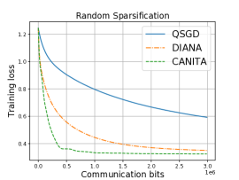
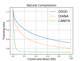
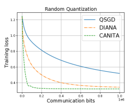
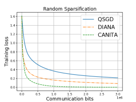
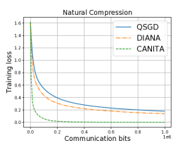
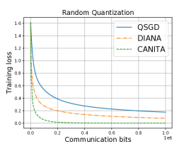
Figure 1: Performance of different methods for three different compressors (random sparsification, natural compression, and random quantization) on the a9a dataset.

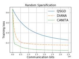
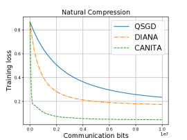
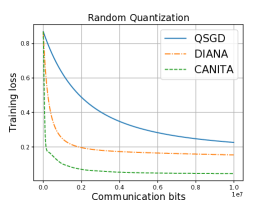
Figure 2: Performance of different methods for three different compressors (random sparsification, natural compression, and random quantization) on the mushrooms dataset.

Figure 3: Performance of different methods for three different compressors (random sparsification, natural compression, and random quantization) on the w8a dataset.

7 Conclusion

In this paper, we proposed CANITA: the first gradient method for distributed general convex optimization provably enjoying the benefits of both communication compression and convergence acceleration. There is very limited work on combing compression and acceleration. Indeed, previous works only focus on the (much simpler) strongly convex setting. We hope that our novel algorithm and analysis can provide new insights and shed light on future work in this line of research. We leave further improvements to future work. For example, one may ask whether our approach can be combined with the benefits provided by multiple local update steps [29, 38, 11, 10, 42], with additional variance reduction techniques [9, 24], and to what extent one can extend our results to structured nonconvex problems [22, 19, 27, 21, 25, 6, 35, 5].

Appendix A Missing Proof for Theorem 1 in Section 5.1

In order to prove Theorem 1, we first formulate six auxiliary results (Lemmas 1–6) in Appendix A.1. The detailed proofs of these lemmas are deferred to Appendix C. Then in Appendix A.2 we show that Theorem 1 follows from Lemma 6.

A.1 Six lemmas

First, we need a useful Lemma 1 which captures the change of the function value after a single gradient update step.

Lemma 1

Suppose that Assumption 1 holds. For any $\beta_{t}>0$, the following equation holds for CANITA (Algorithm 1) for any round $t\geq 0$:

$${\mathbb{E}}\left[f(z^{t+1})\right] \leq{\mathbb{E}}\bigg{[}f(y^{t})+\langle\nabla f(y^{t}),\theta_{t}(x^{*}-x^{t})\rangle+\frac{\theta_{t}^{2}}{\eta_{t}}\left(D^{t}-D^{t+1}\right)$$

$$\qquad\qquad-\left(\frac{\theta_{t}^{2}}{2\eta_{t}}-\frac{L(1+\beta_{t})\theta_{t}^{2}}{2}\right)\|x^{t+1}-x^{t}\|^{2}+\frac{1}{2L\beta_{t}}\|\nabla f(y^{t})-g^{t}\|^{2}\bigg{]}.$$ (15)

Note that

$$z^{t+1}-y^{t}=\theta_{t}(x^{t+1}-x^{t})=-\eta_{t}g^{t}$$

according to the two momentum/interpolation steps of CANITA (see Line 3 and Line 10 of Algorithm 1) and the gradient update step (see Line 9 of Algorithm 1). The proof of Lemma 1 uses these relations and the smoothness Assumption 1.

In the next lemma, we bound the last variance term ${\mathbb{E}}\left[\|\nabla f(y^{t})-g^{t}\|^{2}\right]$ appearing in (15) of Lemma 1. To simplify the notation, from now on we will write

$$Y^{t}:=\frac{1}{n}\sum_{i=1}^{n}\|\nabla f_{i}(w^{t})-\nabla f_{i}(y^{t})\|^{2},$$ (16)

and recall that $H^{t}:=\frac{1}{n}\sum_{i=1}^{n}\|\nabla f_{i}(w^{t})-h_{i}^{t}\|^{2}$ defined in (4).

Lemma 2

If $g^{t}$ is as defined in Line 8 of Algorithm 1, and the compression operator ${\cal C}_{i}^{t}$ satisfies (2) of Definition 2, we have

$${\mathbb{E}}\left[\|\nabla f(y^{t})-g^{t}\|^{2}\right]\leq\frac{2\omega}{n}\left(Y^{t}+H^{t}\right).$$ (17)

This lemma is proved by using the definition of the $\omega$-compression operator (i.e., (2)).

Now, we need to bound the terms $Y^{t}$ and $H^{t}$ in (17) of Lemma 2. We first show how to handle the term $H^{t}$ in the following Lemma 3.

Lemma 3

Suppose that Assumption 1 holds and let $\alpha_{t}\leq\frac{1}{1+\omega}$. According to the probabilistic update of $w^{t+1}$ in Line 11 of Algorithm 1, we have

$$\mathbb{E}\left[H^{t+1}\right] \leq\left(1-\frac{\alpha_{t}}{2}\right)H^{t}+2p_{t}\left(1+\frac{2p_{t}}{\alpha_{t}}\right)Y^{t}+2p_{t}L^{2}\theta_{t}^{2}\left(1+\frac{2p_{t}}{\alpha_{t}}\right){\mathbb{E}}\left[\|x^{t+1}-x^{t}\|^{2}\right].$$ (18)

This lemma is proved by using the update of $w^{t+1}$ (Line 11 of Algorithm 1) and $h_{i}^{t+1}$ (Line 6 of Algorithm 1), the property of $\omega$-compression operator (i.e., (2)), and the smoothness Assumption 1.

To deal with the term $Y^{t}$ in Lemmas 2 and 3, we need the following result.

Lemma 4

Suppose that Assumption 1 holds. For any $y^{t},w^{t}\in{\mathbb{R}}^{d}$, the following inequality holds:

$$Y^{t}\leq 2L\Big{(}f(w^{t})-f(y^{t})-\langle\nabla f(y^{t}),w^{t}-y^{t}\rangle\Big{)}.$$ (19)

The proof of this lemma directly follows from a standard result characterizing the $L$-smoothness of convex functions.

Finally, we also need a result connecting the function values $f(z^{t+1})$ in (15) of Lemma 1 and $f(w^{t+1})$ in (7) of Theorem 1 (recall that $F^{t+1}:=f(w^{t+1})-f(x^{*})$ in (4)).

Lemma 5

According to the probabilistic update of $w^{t+1}$ in Line 11 of Algorithm 1, we have

$${\mathbb{E}}[f(w^{t+1})]=p_{t}{\mathbb{E}}[f(z^{t+1})]+(1-p_{t}){\mathbb{E}}[f(w^{t})].$$ (20)

Now, we combine Lemmas 1–5 to obtain our final key lemma, which describes the recursive form of the objective function value after a single round.

Lemma 6

Suppose that Assumption 1 holds and the compression operators $\{{\cal C}_{i}^{t}\}$ used in Algorithm 1 satisfy (2) of Definition 2. For any two positive sequences $\{\beta_{t}\}$ and $\{\gamma_{t}\}$ such that the probabilities $\{p_{t}\}$ and positive stepsizes $\{\alpha_{t}\},\{\eta_{t}\},\{\theta_{t}\}$ of Algorithm 1 satisfy the following relations

$$\small\alpha_{t}\leq\frac{1}{1+\omega},\qquad\eta_{t}\leq\frac{1}{L\left(1+\beta_{t}+4p_{t}\gamma_{t}\big{(}1+\frac{2p_{t}}{\alpha_{t}}\big{)}\right)}$$ (21)

for all $t\geq 0$, and

$$\small\frac{2\omega}{\beta_{t}n}+4p_{t}\gamma_{t}\Big{(}1+\frac{2p_{t}}{\alpha_{t}}\Big{)}\leq 1-\theta_{t}$$ (22)

for all $t\geq 1$. Then the sequences $\{x^{t},w^{t},h_{i}^{t}\}$ of CANITA (Algorithm 1) for all $t\geq 0$ satisfy the inequality

$$\mathbb{E}\left[F^{t+1}+\frac{\gamma_{t}p_{t}}{L}H^{t+1}\right]\leq{\mathbb{E}}\bigg{[}(1-\theta_{t}p_{t})F^{t}+\Big{(}\frac{\omega}{\beta_{t}n}+\Big{(}1-\frac{\alpha_{t}}{2}\Big{)}\gamma_{t}\Big{)}\frac{p_{t}}{L}H^{t}+\frac{\theta_{t}^{2}p_{t}}{\eta_{t}}\Big{(}D^{t}-D^{t+1}\Big{)}\bigg{]}.$$ (23)

A.2 Proof of Theorem 1

Now, we are ready to prove the main convergence Theorem 1. According to Lemma 6, we know the change of the function value after each round. By dividing (23) with $\frac{\theta_{t}^{2}p_{t}}{\eta_{t}}$ on both sides, we obtain

$$\mathbb{E}\left[\frac{\eta_{t}}{\theta_{t}^{2}p_{t}}F^{t+1}+\frac{\gamma_{t}\eta_{t}}{\theta_{t}^{2}L}H^{t+1}\right]\leq{\mathbb{E}}\bigg{[}\frac{(1-\theta_{t}p_{t})\eta_{t}}{\theta_{t}^{2}p_{t}}F^{t}+\Big{(}\frac{\omega}{\beta_{t}n}+\Big{(}1-\frac{\alpha_{t}}{2}\Big{)}\gamma_{t}\Big{)}\frac{\eta_{t}}{\theta_{t}^{2}L}H^{t}+D^{t}-D^{t+1}\bigg{]}.$$ (24)

Then according to the following conditions on the parameters (see (6) of Theorem 1):

$$\frac{(1-p_{t}\theta_{t})\eta_{t}}{p_{t}\theta_{t}^{2}}\leq\frac{\eta_{t-1}}{p_{t-1}\theta_{t-1}^{2}},\text{~{}~{}and~{}~{}}\Big{(}\frac{\omega}{\beta_{t}n}+\left(1-\frac{\alpha_{t}}{2}\right)\gamma_{t}\Big{)}\frac{\eta_{t}}{\theta_{t}^{2}}\leq\frac{\gamma_{t-1}\eta_{t-1}}{\theta_{t-1}^{2}},~{}~{}\forall t\geq 1.$$ (25)

The proof of Theorem 1 is finished by telescoping (24) from $t=1$ to $T$ via (25) and maintaining the same inequality (24) for $t=0$:

$$\mathbb{E}\left[F^{T+1}+\frac{\gamma_{T}p_{T}}{L}H^{T+1}\right]\leq\frac{\theta_{T}^{2}p_{T}}{\eta_{T}}\bigg{(}\frac{(1-\theta_{0}p_{0})\eta_{0}}{\theta_{0}^{2}p_{0}}F^{0}+\Big{(}\frac{\omega}{\beta_{0}n}+\Big{(}1-\frac{\alpha_{0}}{2}\Big{)}\gamma_{0}\Big{)}\frac{\eta_{0}}{\theta_{0}^{2}L}H^{0}+D^{0}\bigg{)}.$$ (26)

$\square$

Appendix B Missing Proof for Theorem 2 in Section 5.2

In this appendix, we provide the proof for concrete Theorem 2 (which leads to a detailed convergence result). First, let us verify that the choice of parameters (i.e., (10)–(12)) in Theorem 2 satisfies the conditions (i.e., (5) and (6)) in Theorem 1. According to $p_{t}$ and $\alpha_{t}$ in (11) and $\gamma_{t}$ in (10), we have

$$4p_{t}\gamma_{t}\left(1+\frac{2p_{t}}{\alpha_{t}}\right)=\frac{1}{2},~{}~{}\forall t\geq 0.$$ (27)

Then according to (27), $\eta_{t}$ of (12) and $\alpha_{t}$ of (11), the first two conditions in (5) of Theorem 1 are satisfied, i.e.,

$$\eta_{t}\leq\frac{1}{L\left(1+\beta_{t}+4p_{t}\gamma_{t}\big{(}1+\frac{2p_{t}}{\alpha_{t}}\big{)}\right)}\text{~{}~{}and~{}~{}}\alpha_{t}\leq\frac{1}{1+\omega},~{}~{}\forall t\geq 0.$$

Besides, from (10) and (11), we know that $\theta_{t}\leq\frac{1}{3}$ and $\frac{2\omega}{\beta_{t}n}\leq\frac{1}{6}$ for any $t\geq 1$. Combining with (27), then the following condition in (6) of Theorem 1 is satisfied:

$$\frac{2\omega}{\beta_{t}n}+4p_{t}\gamma_{t}\left(1+\frac{2p_{t}}{\alpha_{t}}\right)\leq 1-\theta_{t},~{}~{}\forall t\geq 1.$$

Now, only the following two conditions in (6) of Theorem 1 are remained:

$$\frac{(1-p_{t}\theta_{t})\eta_{t}}{p_{t}\theta_{t}^{2}}\leq\frac{\eta_{t-1}}{p_{t-1}\theta_{t-1}^{2}},\text{~{}~{}and~{}~{}}\Big{(}\frac{\omega}{\beta_{t}n}+\left(1-\frac{\alpha_{t}}{2}\right)\gamma_{t}\Big{)}\frac{\eta_{t}}{\theta_{t}^{2}}\leq\frac{\gamma_{t-1}\eta_{t-1}}{\theta_{t-1}^{2}},~{}~{}\forall t\geq 1.$$ (28)

For the first condition of (28), by plugging the parameter choice $\{p_{t}\}$ and $\{\theta_{t}\}$ of (11), it is sufficient to let

$$\left(1-\frac{3}{t+9(1+b+\omega)}\right)\eta_{t}\leq\left(1-\frac{1}{t+9(1+b+\omega)}\right)^{2}\eta_{t-1},~{}~{}\forall t\geq 1.$$ (29)

For satisfying (29), it is sufficient to choose $\eta_{t}$ as in (12):

$$\eta_{t}=\min\left\{\Big{(}1+\frac{1}{t+9(1+b+\omega)}\Big{)}\eta_{t-1},~{}\frac{1}{L(\beta+3/2)}\right\},~{}~{}\forall t\geq 1.$$ (30)

Similarly, for the second condition of (28), by plugging the parameter choice $\{\theta_{t}\}$ and $\{\alpha_{t}\}$ of (11), it is sufficient to let

$$\Big{(}\frac{\omega}{\beta_{t}n}+\Big{(}1-\frac{1}{2(1+\omega)}\Big{)}\gamma_{t}\Big{)}\eta_{t} \leq\gamma_{t-1}\eta_{t-1}\Big{(}1-\frac{1}{t+9(1+b+\omega)}\Big{)}^{2},~{}~{}\forall t\geq 1.$$ (31)

By plugging $\{\beta_{t}\}$ and $\{\gamma_{t}\}$ of (10) into (31), we have

$$\left(1-\frac{1}{3(1+\omega)}\right)\eta_{t} \leq\eta_{t-1}\left(1-\frac{1}{t+9(1+b+\omega)}\right)^{2},~{}~{}\forall t\geq 1.$$ (32)

Note that the choice of $\eta_{t}$ in (30) also satisfies (32).

Now, we have verified that all conditions of Theorem 1 are satisfied with the parameter choice in Theorem 2. Next, we obtain the detailed convergence results of CANITA by using this choice of parameters. According to Theorem 1, we know that the following equation holds for any $T>0$:

$$\mathbb{E}\left[F^{T+1}+\frac{\gamma_{T}p_{T}}{L}H^{T+1}\right]\leq\frac{\theta_{T}^{2}p_{T}}{\eta_{T}}\bigg{(}\frac{(1-\theta_{0}p_{0})\eta_{0}}{\theta_{0}^{2}p_{0}}F^{0}+\Big{(}\frac{\omega}{\beta_{0}n}+\Big{(}1-\frac{\alpha_{0}}{2}\Big{)}\gamma_{0}\Big{)}\frac{\eta_{0}}{\theta_{0}^{2}L}H^{0}+D^{0}\bigg{)}.$$ (33)

According to (11), we have

$$\theta_{T}^{2}p_{T}=\frac{9(1+b)}{(T+9(1+b+\omega))^{2}}.$$ (34)

According to (30), we have

$$\eta_{T} =\min\left\{\frac{T+9(1+b+\omega)}{9(1+b+\omega)}\eta_{0},~{}\frac{1}{L(\beta+3/2)}\right\}$$

$$=\min\left\{\frac{T+9(1+b+\omega)}{9(1+b+\omega)}\frac{1}{L(\beta_{0}+3/2)},~{}\frac{1}{L(\beta+3/2)}\right\}$$

$$=\min\left\{\frac{(T+9(1+b+\omega))(1+b)}{162(1+b+\omega)^{3}},~{}\frac{1}{L(\beta+3/2)}\right\},$$ (35)

where (35) uses the appropriate $\beta_{0}=\frac{9(1+b+\omega)^{2}}{(1+b)L}$ chosen in (10) of Theorem 2. Besides, according to the initial values of the parameters, we can simplify the right-hand-side of (33) with $\frac{(1-\theta_{0}p_{0})\eta_{0}}{\theta_{0}^{2}p_{0}}\leq 1$ and $\left(1-\frac{\alpha_{0}}{2}\right)\gamma_{0}\frac{\eta_{0}}{\theta_{0}^{2}L}\leq 1$.

Now we plug (34) and (35) into (33) and omit the constant to obtain

$$\mathbb{E}\left[F^{T+1}\right] \leq O\left(\max\left\{\frac{(1+b+\omega)^{3}}{(T+9(1+b+\omega))^{3}},~{}\frac{(1+b)(\beta+3/2)L}{(T+9(1+b+\omega))^{2}}\right\}\right)$$

$$\leq O\left(\max\left\{\frac{(1+b+\omega)^{3}}{T^{3}},~{}\frac{(1+b)(\beta+3/2)L}{T^{2}}\right\}\right)$$

$$\leq O\left(\max\left\{\frac{(1+\omega)^{3}}{T^{3}},~{}\frac{(1+\sqrt{\omega(1+\omega)^{2}/n})L}{T^{2}}\right\}\right)$$ (36)

$$=O\left(\frac{(1+\sqrt{\omega^{3}/n})L}{T^{2}}+\frac{\omega^{3}}{T^{3}}\right),$$ (37)

where (36) uses $b=\min\Big{\{}\omega,\sqrt{\frac{\omega(1+\omega)^{2}}{n}}\Big{\}}$ and $\beta$ of (10) . Following from (37), we know that the number of communication rounds for CANITA (Algorithm 1) to find an $\epsilon$-solution such that

$${\mathbb{E}}\left[f(w^{T+1})-f(x^{*})\right]\overset{\eqref{eq:F,H,D}}{:=}{\mathbb{E}}\left[F^{T+1}\right]\leq\epsilon$$

is at most

$$T=O\left(\sqrt{\bigg{(}1+\sqrt{\frac{\omega^{3}}{n}}\bigg{)}\frac{L}{\epsilon}}+\omega\left(\frac{1}{\epsilon}\right)^{\frac{1}{3}}\right).$$

$\square$

Appendix C Missing Proofs for Six Lemmas in Appendix A.1

In Appendix A, we provided the proof of Theorem 1 using six lemmas. Now we present the omitted proofs for these Lemmas 1–6 in Appendices C.1–C.6, respectively.

C.1 Proof of Lemma 1

According to the $L$-smoothness of $f$ (Assumption 1), we have

$${\mathbb{E}}\left[f(z^{t+1})\right]$$

$$\leq{\mathbb{E}}\bigg{[}f(y^{t})+\langle\nabla f(y^{t}),z^{t+1}-y^{t}\rangle+\frac{L}{2}\|z^{t+1}-y^{t}\|^{2}\bigg{]}$$

$$={\mathbb{E}}\bigg{[}f(y^{t})+\langle\nabla f(y^{t}),\theta_{t}(x^{t+1}-x^{t})\rangle+\frac{L\theta_{t}^{2}}{2}\|x^{t+1}-x^{t}\|^{2}\bigg{]}$$ (38)

$$={\mathbb{E}}\bigg{[}f(y^{t})+\langle\nabla f(y^{t})-g^{t},\theta_{t}(x^{t+1}-x^{t})\rangle+\langle g^{t},\theta_{t}(x^{t+1}-x^{t})\rangle+\frac{L\theta_{t}^{2}}{2}\|x^{t+1}-x^{t}\|^{2}\bigg{]}$$

$$\leq{\mathbb{E}}\bigg{[}f(y^{t})+\frac{1}{2L\beta_{t}}\|\nabla f(y^{t})-g^{t}\|^{2}+\frac{L\beta_{t}\theta_{t}^{2}}{2}\|x^{t+1}-x^{t}\|^{2}+\frac{L\theta_{t}^{2}}{2}\|x^{t+1}-x^{t}\|^{2}$$

$$\qquad\qquad\qquad+\langle g^{t},\theta_{t}(x^{t+1}-x^{t})\rangle\bigg{]}$$ (39)

$$={\mathbb{E}}\bigg{[}f(y^{t})+\frac{1}{2L\beta_{t}}\|\nabla f(y^{t})-g^{t}\|^{2}+\frac{L(1+\beta_{t})\theta_{t}^{2}}{2}\|x^{t+1}-x^{t}\|^{2}$$

$$\qquad\qquad\qquad+\langle g^{t},\theta_{t}(x^{*}-x^{t})\rangle+\langle g^{t},\theta_{t}(x^{t+1}-x^{*})\rangle\bigg{]}$$

$$={\mathbb{E}}\bigg{[}f(y^{t})+\frac{1}{2L\beta_{t}}\|\nabla f(y^{t})-g^{t}\|^{2}+\frac{L(1+\beta_{t})\theta_{t}^{2}}{2}\|x^{t+1}-x^{t}\|^{2}+\langle\nabla f(y^{t}),\theta_{t}(x^{*}-x^{t})\rangle$$

$$\qquad\qquad\qquad+\langle g^{t},\theta_{t}(x^{t+1}-x^{*})\rangle\bigg{]}$$ (40)

$$={\mathbb{E}}\bigg{[}f(y^{t})+\frac{1}{2L\beta_{t}}\|\nabla f(y^{t})-g^{t}\|^{2}+\frac{L(1+\beta_{t})\theta_{t}^{2}}{2}\|x^{t+1}-x^{t}\|^{2}+\langle\nabla f(y^{t}),\theta_{t}(x^{*}-x^{t})\rangle$$

$$\qquad\qquad\qquad+\frac{\theta_{t}^{2}}{\eta_{t}}\langle x^{t}-x^{t+1},x^{t+1}-x^{*}\rangle\bigg{]}$$ (41)

$$={\mathbb{E}}\bigg{[}f(y^{t})+\frac{1}{2L\beta_{t}}\|\nabla f(y^{t})-g^{t}\|^{2}+\frac{L(1+\beta_{t})\theta_{t}^{2}}{2}\|x^{t+1}-x^{t}\|^{2}+\langle\nabla f(y^{t}),\theta_{t}(x^{*}-x^{t})\rangle$$

$$\qquad\qquad\qquad+\frac{\theta_{t}^{2}}{2\eta_{t}}\big{(}\|x^{t}-x^{*}\|^{2}-\|x^{t}-x^{t+1}\|^{2}-\|x^{t+1}-x^{*}\|^{2}\big{)}\bigg{]}$$

$$={\mathbb{E}}\bigg{[}f(y^{t})+\langle\nabla f(y^{t}),\theta_{t}(x^{*}-x^{t})\rangle+\frac{\theta_{t}^{2}}{2\eta_{t}}\big{(}\|x^{t}-x^{*}\|^{2}-\|x^{t+1}-x^{*}\|^{2}\big{)}$$

$$\qquad\qquad\qquad-\Big{(}\frac{\theta_{t}^{2}}{2\eta_{t}}-\frac{L(1+\beta_{t})\theta_{t}^{2}}{2}\Big{)}\|x^{t+1}-x^{t}\|^{2}+\frac{1}{2L\beta_{t}}\|\nabla f(y^{t})-g^{t}\|^{2}\bigg{]},$$

where (38) holds since $z^{t+1}-y^{t}=\theta_{t}(x^{t+1}-x^{t})$ according to the two momentum/interpolation steps of CANITA (see Line 3 and Line 10 of Algorithm 1), (39) uses Young’s inequality with any $\beta_{t}>0$, (40) holds due to ${\mathbb{E}}[g^{t}]=\nabla f(y^{t})$ since the compression is unbiased from (2), and (41) holds according to the gradient update step $x^{t+1}=x^{t}-\frac{\eta_{t}}{\theta_{t}}g^{t}$ (see Line 9 of Algorithm 1). $\square$

C.2 Proof of Lemma 2

This lemma is proved as follows:

$${\mathbb{E}}\left[\|\nabla f(y^{t})-g^{t}\|^{2}\right] ={\mathbb{E}}\left[\left\|\frac{1}{n}\sum_{i=1}^{n}\Big{(}{\cal C}_{i}^{t}(\nabla f_{i}(y^{t})-h_{i}^{t})+h_{i}^{t}-\nabla f_{i}(y^{t})\Big{)}\right\|^{2}\right]$$

$$=\frac{1}{n^{2}}\sum_{i=1}^{n}{\mathbb{E}}\left[\left\|{\cal C}_{i}^{t}(\nabla f_{i}(y^{t})-h_{i}^{t})+h_{i}^{t}-\nabla f_{i}(y^{t})\right\|^{2}\right]$$

$$\leq\frac{\omega}{n^{2}}\sum_{i=1}^{n}\|\nabla f_{i}(y^{t})-h_{i}^{t}\|^{2}$$ (42)

$$\leq\frac{2\omega}{n^{2}}\sum_{i=1}^{n}\|\nabla f_{i}(y^{t})-\nabla f_{i}(w^{t})\|^{2}+\frac{2\omega}{n^{2}}\sum_{i=1}^{n}\|\nabla f_{i}(w^{t})-h_{i}^{t}\|^{2},$$ (43)

where (42) follows from the definition of $\omega$-compression operator (i.e., (2)), and the last inequality (43) uses Cauchy-Schwarz inequality. $\square$

C.3 Proof of Lemma 3

Firstly, according to the probabilistic update of $w^{t+1}$ (see Line 11 of Algorithm 1) and recalling that $H^{t}:=\frac{1}{n}\sum_{i=1}^{n}\|\nabla f_{i}(w^{t})-h_{i}^{t}\|^{2}$ defined in (4), we get

$$\mathbb{E}\left[H^{t+1}\right]$$

$$=\frac{p_{t}}{n}\sum_{i=1}^{n}\mathbb{E}\left[\left\|\nabla f_{i}(z^{t+1})-h_{i}^{t+1}\right\|^{2}\right]+\frac{1-p_{t}}{n}\sum_{i=1}^{n}\mathbb{E}\left[\left\|\nabla f_{i}(w^{t})-h_{i}^{t+1}\right\|^{2}\right]$$

$$\leq\left(1+\frac{2p_{t}}{\alpha_{t}}\right)\frac{p_{t}}{n}\sum_{i=1}^{n}\mathbb{E}\left[\left\|\nabla f_{i}(z^{t+1})-\nabla f_{i}(w^{t})\right\|^{2}\right]+\left(1+\frac{\alpha_{t}}{2p_{t}}\right)\frac{p_{t}}{n}\sum_{i=1}^{n}\mathbb{E}\left[\left\|\nabla f_{i}(w^{t})-h_{i}^{t+1}\right\|^{2}\right]$$

$$\qquad\qquad\qquad+\frac{1-p_{t}}{n}\sum_{i=1}^{n}\mathbb{E}\left[\left\|\nabla f_{i}(w^{t})-h_{i}^{t+1}\right\|^{2}\right].$$ (44)

$$\leq\left(1+\frac{2p_{t}}{\alpha_{t}}\right)\frac{p_{t}}{n}\sum_{i=1}^{n}\mathbb{E}\left[\left\|\nabla f_{i}(z^{t+1})-\nabla f_{i}(w^{t})\right\|^{2}\right]+\Big{(}1+\frac{\alpha_{t}}{2}\Big{)}\Big{(}1-2\alpha_{t}+\alpha_{t}^{2}(1+\omega)\Big{)}H^{t}$$ (45)

$$\leq\left(1+\frac{2p_{t}}{\alpha_{t}}\right)\frac{p_{t}}{n}\sum_{i=1}^{n}\mathbb{E}\left[\left\|\nabla f_{i}(z^{t+1})-\nabla f_{i}(w^{t})\right\|^{2}\right]+\left(1-\frac{\alpha_{t}}{2}\right)H^{t}$$ (46)

$$\leq\left(1+\frac{2p_{t}}{\alpha_{t}}\right)\frac{2p_{t}}{n}\sum_{i=1}^{n}\mathbb{E}\left[\left\|\nabla f_{i}(z^{t+1})-\nabla f_{i}(y^{t})\right\|^{2}+\left\|\nabla f_{i}(y^{t})-\nabla f_{i}(w^{t})\right\|^{2}\right]+\left(1-\frac{\alpha_{t}}{2}\right)H^{t}$$ (47)

$$\leq\left(1+\frac{2p_{t}}{\alpha_{t}}\right)\frac{2p_{t}}{n}\sum_{i=1}^{n}\mathbb{E}\left[L^{2}\left\|z^{t+1}-y^{t}\right\|^{2}+\left\|\nabla f_{i}(y^{t})-\nabla f_{i}(w^{t})\right\|^{2}\right]+\left(1-\frac{\alpha_{t}}{2}\right)H^{t}$$ (48)

$$\leq 2p_{t}L^{2}\theta_{t}^{2}\left(1+\frac{2p_{t}}{\alpha_{t}}\right){\mathbb{E}}\left[\|x^{t+1}-x^{t}\|^{2}\right]+2p_{t}\left(1+\frac{2p_{t}}{\alpha_{t}}\right)Y^{t}+\left(1-\frac{\alpha_{t}}{2}\right)H^{t},$$ (49)

where (44) uses Young’s inequality, (45) uses the update of local shifts $h_{i}^{t+1}=h_{i}^{t}+\alpha_{t}{\cal C}_{i}^{t}(\nabla f_{i}(w^{t})-h_{i}^{t})$ (see Line 6 of Algorithm 1) and the property of $\omega$-compression operator (i.e., (2)), (46) uses $\alpha_{t}\leq\nicefrac{{1}}{{(1+\omega)}}$, (47) uses Cauchy-Schwarz inequality, (48) uses the $L$-smoothness of $f_{i}$ (Assumption 1), and the last inequality (49) holds since $z^{t+1}-y^{t}=\theta_{t}(x^{t+1}-x^{t})$ according to the two interpolation steps of CANITA (see Line 3 and Line 10 of Algorithm 1). $\square$

C.4 Proof of Lemma 4

This lemma directly follows from a standard result under Assumption 1. According to e.g. Lemma 1 of [18] or Lemma 5 of [20], we have

$$\frac{1}{2L}\|\nabla f_{i}(w^{t})-\nabla f_{i}(y^{t})\|^{2}\leq f_{i}(w^{t})-f_{i}(y^{t})-\langle\nabla f_{i}(y^{t}),w^{t}-y^{t}\rangle.$$ (50)

Then, the result (19) is obtained by summing up (50) for all $i\in[n]$ and noting $f(x):=\frac{1}{n}\sum_{i=1}^{n}f_{i}(x)$ (see (1)) and $Y^{t}:=\frac{1}{n}\sum_{i=1}^{n}\|\nabla f_{i}(w^{t})-\nabla f_{i}(y^{t})\|^{2}$ (see (16)). $\square$

C.5 Proof of Lemma 5

The lemma follows directly from the probabilistic update of $w^{t+1}$; see Line 11 of Algorithm 1. $\square$

C.6 Proof of Lemma 6

Now, we provide the detailed proof for the key Lemma 6 by using previous Lemmas 1–5. First, we plug (17) of Lemma 2 into (15) of Lemma 1 to obtain

$${\mathbb{E}}\left[f(z^{t+1})\right] \leq{\mathbb{E}}\bigg{[}f(y^{t})+\langle\nabla f(y^{t}),\theta_{t}(x^{*}-x^{t})\rangle+\frac{\theta_{t}^{2}}{\eta_{t}}\big{(}D^{t}-D^{t+1}\big{)}$$

$$\qquad-\left(\frac{\theta_{t}^{2}}{2\eta_{t}}-\frac{L(1+\beta_{t})\theta_{t}^{2}}{2}\right)\|x^{t+1}-x^{t}\|^{2}+\frac{\omega}{L\beta_{t}n}Y^{t}+\frac{\omega}{L\beta_{t}n}H^{t}\bigg{]}.$$ (51)

Then, we add (51) and $\frac{\gamma_{t}}{L}\times$ (18) of Lemma 3 to get

$$\mathbb{E}\left[f(z^{t+1})+\frac{\gamma_{t}}{L}H^{t+1}\right]$$

$$\leq{\mathbb{E}}\bigg{[}f(y^{t})+\langle\nabla f(y^{t}),\theta_{t}(x^{*}-x^{t})\rangle+\frac{\theta_{t}^{2}}{\eta_{t}}\big{(}D^{t}-D^{t+1}\big{)}$$

$$\qquad\qquad-\left(\frac{\theta_{t}^{2}}{2\eta_{t}}-\frac{L(1+\beta_{t})\theta_{t}^{2}}{2}\right)\|x^{t+1}-x^{t}\|^{2}+\frac{\omega}{L\beta_{t}n}Y^{t}+\frac{\omega}{L\beta_{t}n}H^{t}$$

$$\qquad\qquad+\left(1-\frac{\alpha_{t}}{2}\right)\frac{\gamma_{t}}{L}H^{t}+\left(1+\frac{2p_{t}}{\alpha_{t}}\right)\frac{2p_{t}\gamma_{t}}{L}Y^{t}+2p_{t}\gamma_{t}L\theta_{t}^{2}\left(1+\frac{2p_{t}}{\alpha_{t}}\right)\|x^{t+1}-x^{t}\|^{2}\bigg{]}$$

$$={\mathbb{E}}\bigg{[}f(y^{t})+\langle\nabla f(y^{t}),\theta_{t}(x^{*}-x^{t})\rangle+\frac{\theta_{t}^{2}}{\eta_{t}}\big{(}D^{t}-D^{t+1}\big{)}$$

$$\qquad\qquad-\left(\frac{\theta_{t}^{2}}{2\eta_{t}}-\frac{L(1+\beta_{t})\theta_{t}^{2}}{2}-2p_{t}\gamma_{t}L\theta_{t}^{2}\Big{(}1+\frac{2p_{t}}{\alpha_{t}}\Big{)}\right)\|x^{t+1}-x^{t}\|^{2}$$

$$\qquad\qquad+\left(\frac{\omega}{\beta_{t}n}+\left(1-\frac{\alpha_{t}}{2}\right)\gamma_{t}\right)\frac{1}{L}H^{t}+\left(\frac{2\omega}{\beta_{t}n}+4p_{t}\gamma_{t}\Big{(}1+\frac{2p_{t}}{\alpha_{t}}\Big{)}\right)\frac{1}{2L}Y^{t}\bigg{]}$$

$$\leq{\mathbb{E}}\bigg{[}f(y^{t})+\langle\nabla f(y^{t}),\theta_{t}(x^{*}-x^{t})\rangle+\frac{\theta_{t}^{2}}{\eta_{t}}\left(D^{t}-D^{t+1}\right)+\left(\frac{\omega}{\beta_{t}n}+\left(1-\frac{\alpha_{t}}{2}\right)\gamma_{t}\right)\frac{1}{L}H^{t}$$

$$\qquad\qquad+\left(\frac{2\omega}{\beta_{t}n}+4p_{t}\gamma_{t}\Big{(}1+\frac{2p_{t}}{\alpha_{t}}\Big{)}\right)\frac{1}{2L}Y^{t}\bigg{]}$$ (52)

$$\leq{\mathbb{E}}\bigg{[}f(y^{t})+\langle\nabla f(y^{t}),\theta_{t}(x^{*}-x^{t})\rangle+\frac{\theta_{t}^{2}}{\eta_{t}}\big{(}D^{t}-D^{t+1}\big{)}+\left(\frac{\omega}{\beta_{t}n}+\left(1-\frac{\alpha_{t}}{2}\right)\gamma_{t}\right)\frac{1}{L}H^{t}$$

$$\qquad\qquad+\frac{1-\theta_{t}}{2L}Y^{t}\bigg{]}$$ (53)

$$\leq{\mathbb{E}}\bigg{[}f(y^{t})+\langle\nabla f(y^{t}),\theta_{t}(x^{*}-x^{t})\rangle+\frac{\theta_{t}^{2}}{\eta_{t}}\big{(}D^{t}-D^{t+1}\big{)}+\left(\frac{\omega}{\beta_{t}n}+\left(1-\frac{\alpha_{t}}{2}\right)\gamma_{t}\right)\frac{1}{L}H^{t}$$

$$\qquad\qquad+(1-\theta_{t})\Big{(}f(w^{t})-f(y^{t})-\langle\nabla f(y^{t}),w^{t}-y^{t}\rangle\Big{)}\bigg{]}$$ (54)

$$={\mathbb{E}}\bigg{[}f(y^{t})+\langle\nabla f(y^{t}),\theta_{t}(x^{*}-x^{t})\rangle+\frac{\theta_{t}^{2}}{\eta_{t}}\big{(}D^{t}-D^{t+1}\big{)}+\left(\frac{\omega}{\beta_{t}n}+\left(1-\frac{\alpha_{t}}{2}\right)\gamma_{t}\right)\frac{1}{L}H^{t}$$

$$\qquad\qquad+(1-\theta_{t})\left(f(w^{t})-f(y^{t})\right)-\theta_{t}\langle\nabla f(y^{t}),y^{t}-x^{t}\rangle\bigg{]}$$ (55)

$$\leq{\mathbb{E}}\bigg{[}(1-\theta_{t})f(w^{t})+\theta_{t}f(x^{*})+\frac{\theta_{t}^{2}}{\eta_{t}}\left(D^{t}-D^{t+1}\right)+\left(\frac{\omega}{\beta_{t}n}+\left(1-\frac{\alpha_{t}}{2}\right)\gamma_{t}\right)\frac{1}{L}H^{t}\bigg{]},$$ (56)

where (52) holds by letting $\eta_{t}\leq\frac{1}{L\big{(}1+\beta_{t}+4p_{t}\gamma_{t}(1+2p_{t}/\alpha_{t})\big{)}}$, (53) holds by letting $\frac{2\omega}{\beta_{t}n}+4p_{t}\gamma_{t}(1+\frac{2p_{t}}{\alpha_{t}})\leq 1-\theta_{t}$, (54) follows from (19) of Lemma 4, (55) holds since $y^{t}=\theta_{t}x^{t}+(1-\theta_{t})w^{t}$ (see Line 3 of Algorithm 1), and the last inequality (56) uses the convexity of $f$. Also note that (53) from (52) uses $\frac{2\omega}{\beta_{t}n}+4p_{t}\gamma_{t}(1+\frac{2p_{t}}{\alpha_{t}})\leq 1-\theta_{t}$, however this condition is only needed for $t\geq 1$, i.e., it is not needed for the case $t=0$ since $Y^{0}=0$ from $y^{0}=w^{0}=x^{0}$. The function and inner product terms will also perform the same result in the final (56) since $y^{0}=w^{0}=x^{0}$.

The proof of Lemma 6 is finished by adding $\eqref{eq:use-convex-main}\times p_{t}$ and (20) of Lemma 5 to obtain (23). $\square$

References

- Alistarh et al. [2017] Dan Alistarh, Demjan Grubic, Jerry Li, Ryota Tomioka, and Milan Vojnovic. QSGD: Communication-efficient SGD via gradient quantization and encoding. In Advances in Neural Information Processing Systems, pages 1709–1720, 2017.
- Allen-Zhu [2017] Zeyuan Allen-Zhu. Katyusha: The first direct acceleration of stochastic gradient methods. In Proceedings of the 49th Annual ACM SIGACT Symposium on Theory of Computing, pages 1200–1205. ACM, 2017.
- Beznosikov et al. [2020] Aleksandr Beznosikov, Samuel Horváth, Peter Richtárik, and Mher Safaryan. On biased compression for distributed learning. arXiv:2002.12410, 2020.
- Chang and Lin [2011] Chih-Chung Chang and Chih-Jen Lin. Libsvm: A library for support vector machines. ACM Transactions on Intelligent Systems and Technology (TIST), 2(3):1–27, 2011.
- Fatkhullin et al. [2021] Ilyas Fatkhullin, Igor Sokolov, Eduard Gorbunov, Zhize Li, and Peter Richtárik. EF21 with bells & whistles: Practical algorithmic extensions of modern error feedback. arXiv preprint arXiv:2110.03294, 2021.
- Gorbunov et al. [2021] Eduard Gorbunov, Konstantin Burlachenko, Zhize Li, and Peter Richtárik. MARINA: Faster non-convex distributed learning with compression. In International Conference on Machine Learning, pages 3788–3798. PMLR, arXiv:2102.07845, 2021.
- Hanzely et al. [2018] Filip Hanzely, Konstantin Mishchenko, and Peter Richtárik. SEGA: variance reduction via gradient sketching. In Advances in Neural Information Processing Systems 31, pages 2082–2093, 2018.
- Horváth et al. [2019a] Samuel Horváth, Chen-Yu Ho, Ľudovít Horváth, Atal Narayan Sahu, Marco Canini, and Peter Richtárik. Natural compression for distributed deep learning. arXiv preprint arXiv:1905.10988, 2019a.
- Horváth et al. [2019b] Samuel Horváth, Dmitry Kovalev, Konstantin Mishchenko, Sebastian Stich, and Peter Richtárik. Stochastic distributed learning with gradient quantization and variance reduction. arXiv preprint arXiv:1904.05115, 2019b.
- Karimireddy et al. [2020] Sai Praneeth Karimireddy, Satyen Kale, Mehryar Mohri, Sashank Reddi, Sebastian Stich, and Ananda Theertha Suresh. SCAFFOLD: Stochastic controlled averaging for federated learning. In International Conference on Machine Learning, pages 5132–5143. PMLR, 2020.
- Khaled et al. [2020a] Ahmed Khaled, Konstantin Mishchenko, and Peter Richtárik. Tighter theory for local SGD on identical and heterogeneous data. In International Conference on Artificial Intelligence and Statistics, pages 4519–4529. PMLR, 2020a.
- Khaled et al. [2020b] Ahmed Khaled, Othmane Sebbouh, Nicolas Loizou, Robert M Gower, and Peter Richtárik. Unified analysis of stochastic gradient methods for composite convex and smooth optimization. arXiv preprint arXiv:2006.11573, 2020b.
- Khirirat et al. [2018] Sarit Khirirat, Hamid Reza Feyzmahdavian, and Mikael Johansson. Distributed learning with compressed gradients. arXiv preprint arXiv:1806.06573, 2018.
- Kingma and Ba [2014] Diederik P. Kingma and Jimmy Ba. Adam: a method for stochastic optimization. In The 3rd International Conference on Learning Representations, 2014.
- Konečný et al. [2016] Jakub Konečný, H. Brendan McMahan, Felix Yu, Peter Richtárik, Ananda Theertha Suresh, and Dave Bacon. Federated learning: strategies for improving communication efficiency. In NIPS Private Multi-Party Machine Learning Workshop, 2016.
- Kovalev et al. [2020] Dmitry Kovalev, Samuel Horváth, and Peter Richtárik. Don’t jump through hoops and remove those loops: SVRG and Katyusha are better without the outer loop. In Proceedings of the 31st International Conference on Algorithmic Learning Theory, 2020.
- Lan and Zhou [2015] Guanghui Lan and Yi Zhou. An optimal randomized incremental gradient method. arXiv preprint arXiv:1507.02000, 2015.
- Lan et al. [2019] Guanghui Lan, Zhize Li, and Yi Zhou. A unified variance-reduced accelerated gradient method for convex optimization. In Advances in Neural Information Processing Systems, pages 10462–10472, 2019.
- Li [2019] Zhize Li. SSRGD: Simple stochastic recursive gradient descent for escaping saddle points. In Advances in Neural Information Processing Systems, pages 1521–1531, 2019.
- Li [2021a] Zhize Li. ANITA: An Optimal Loopless Accelerated Variance-Reduced Gradient Method. arXiv preprint arXiv:2103.11333, 2021a.
- Li [2021b] Zhize Li. A Short Note of PAGE: Optimal Convergence Rates for Nonconvex Optimization. arXiv preprint arXiv:2106.09663, 2021b.
- Li and Li [2018] Zhize Li and Jian Li. A simple proximal stochastic gradient method for nonsmooth nonconvex optimization. In Advances in Neural Information Processing Systems, pages 5569–5579, 2018.
- Li and Li [2020] Zhize Li and Jian Li. A fast Anderson-Chebyshev acceleration for nonlinear optimization. In International Conference on Artificial Intelligence and Statistics, pages 1047–1057. PMLR, arXiv:1809.02341, 2020.
- Li and Richtárik [2020] Zhize Li and Peter Richtárik. A unified analysis of stochastic gradient methods for nonconvex federated optimization. arXiv preprint arXiv:2006.07013, 2020.
- Li and Richtárik [2021] Zhize Li and Peter Richtárik. ZeroSARAH: Efficient nonconvex finite-sum optimization with zero full gradient computation. arXiv preprint arXiv:2103.01447, 2021.
- Li et al. [2020] Zhize Li, Dmitry Kovalev, Xun Qian, and Peter Richtárik. Acceleration for compressed gradient descent in distributed and federated optimization. In International Conference on Machine Learning, pages 5895–5904. PMLR, arXiv:2002.11364, 2020.
- Li et al. [2021] Zhize Li, Hongyan Bao, Xiangliang Zhang, and Peter Richtárik. PAGE: A simple and optimal probabilistic gradient estimator for nonconvex optimization. In International Conference on Machine Learning, pages 6286–6295. PMLR, arXiv:2008.10898, 2021.
- Lin et al. [2015] Hongzhou Lin, Julien Mairal, and Zaid Harchaoui. A universal catalyst for first-order optimization. In Advances in Neural Information Processing Systems, pages 3384–3392, 2015.
- McMahan et al. [2017] H Brendan McMahan, Eider Moore, Daniel Ramage, Seth Hampson, and Blaise Agüera y Arcas. Communication-efficient learning of deep networks from decentralized data. In International Conference on Artificial Intelligence and Statistics, pages 1273–1282. PMLR, 2017.
- Mishchenko et al. [2019] Konstantin Mishchenko, Eduard Gorbunov, Martin Takáč, and Peter Richtárik. Distributed learning with compressed gradient differences. arXiv preprint arXiv:1901.09269, 2019.
- Nesterov [1983] Yurii Nesterov. A method for unconstrained convex minimization problem with the rate of convergence . In Doklady AN USSR, volume 269, pages 543–547, 1983.
- Nesterov [2004] Yurii Nesterov. Introductory lectures on convex optimization: a basic course. Kluwer Academic Publishers, 2004.
- Polyak [1964] Boris T Polyak. Some methods of speeding up the convergence of iteration methods. Ussr computational mathematics and mathematical physics, 4(5):1–17, 1964.
- Qian et al. [2020] Xun Qian, Peter Richtárik, and Tong Zhang. Error compensated distributed SGD can be accelerated. arXiv preprint arXiv:2010.00091, 2020.
- Richtárik et al. [2021] Peter Richtárik, Igor Sokolov, and Ilyas Fatkhullin. EF21: A new, simpler, theoretically better, and practically faster error feedback. arXiv preprint arXiv:2106.05203, 2021.
- Safaryan et al. [2021] Mher Safaryan, Egor Shulgin, and Peter Richtárik. Uncertainty principle for communication compression in distributed and federated learning and the search for an optimal compressor. Information and Inference: A Journal of the IMA, 2021.
- Seide et al. [2014] Frank Seide, Hao Fu, Jasha Droppo, Gang Li, and Dong Yu. 1-bit stochastic gradient descent and its application to data-parallel distributed training of speech DNNs. In Fifteenth Annual Conference of the International Speech Communication Association, 2014.
- Stich [2019] Sebastian U. Stich. Local SGD converges fast and communicates little. In International Conference on Learning Representations, 2019.
- Stich et al. [2018] Sebastian U. Stich, Jean-Baptiste Cordonnier, and Martin Jaggi. Sparsified SGD with memory. In Advances in Neural Information Processing Systems, pages 4447–4458, 2018.
- Wangni et al. [2018] Jianqiao Wangni, Jialei Wang, Ji Liu, and Tong Zhang. Gradient sparsification for communication-efficient distributed optimization. In Advances in Neural Information Processing Systems, pages 1306–1316, 2018.
- Ye et al. [2020] Tian Ye, Peijun Xiao, and Ruoyu Sun. DEED: A general quantization scheme for communication efficiency in bits. arXiv preprint arXiv:2006.11401, 2020.
- Zhao et al. [2021] Haoyu Zhao, Zhize Li, and Peter Richtárik. FedPAGE: A fast local stochastic gradient method for communication-efficient federated learning. arXiv preprint arXiv:2108.04755, 2021.