Using Shape Constraints for Improving Symbolic Regression Models

Abstract

We describe and analyze algorithms for shape-constrained symbolic regression, which allows the inclusion of prior knowledge about the shape of the regression function. This is relevant in many areas of engineering – in particular whenever a data-driven model obtained from measurements must have certain properties (e.g. positivity, monotonicity or convexity/concavity). We implement shape constraints using a soft-penalty approach which uses multi-objective algorithms to minimize constraint violations and training error. We use the non-dominated sorting genetic algorithm (NSGA-II) as well as the multi-objective evolutionary algorithm based on decomposition (MOEA/D). We use a set of models from physics textbooks to test the algorithms and compare against earlier results with single-objective algorithms. The results show that all algorithms are able to find models which conform to all shape constraints. Using shape constraints helps to improve extrapolation behavior of the models.

[hag]organization=Josef Ressel Center for Symbolic Regression, University of Applied Sciences Upper Austria, addressline=Softwarepark 11, city=Hagenberg, postcode=4232, country=Austria

[bra]organization=Center for Mathematics, Computation and Cognition (CMCC), Heuristics, Analysis and Learning Laboratory (HAL), Federal University of ABC, city=Santo Andre, country=Brazil

1 Introduction

Modeling of dynamic and complex systems often requires adherence to certain physical behaviors to ensure that the resulting model is trustworthy. A model that adheres to the desired physical laws is essential when studying the control of physical systems since it ensures that the resulting model has a predictable behavior and can be validated and understood by domain experts. Due to the high complexity of such systems, it is usually impossible to model them based on first principles alone, thus requiring empirical data-based modeling. The integration of physical domain knowledge with data-based empirical modeling is a relatively new and not fully-explored, although increasingly important area of research [3].

Symbolic regression (SR) searches for models expressed as formulas whereby the algorithm identifies the model structure and parameters simultaneously. Even though the approach is data-based, it opens the possibility to find short expressions similar to white-box models derived from first principles. Evolutionary algorithms represent a well-known approach for this task. In [18], SR was further extended to constrain the search space with models that have desired physical properties. We have described such constraints by measuring properties of the shape of the model, such as monotonicity and convexity, using interval arithmetic. We proposed shape-constrained symbolic regression (SCSR) [18] as a supervised learning approach for finding SR models.

1.1 Objectives

In this paper, we extend [18] by using multi-objective approaches to find a set of solutions that minimize both approximation error and soft-penalties incurred by constraint violations. Furthermore, we investigate how the extrapolation behavior is affected by shape constraints. We hypothesize that shape constraints can help find more accurate regression models with improved extrapolation ability, especially under the presence of noise in the training data.

The broader goal of this project is to integrate domain knowledge into SR algorithms to ensure that the returned model has a better correspondence to the actual underlying physical conditions of the system.

Specifically for this paper, we have two objectives. The first one is to improve the search process of a constrained model using multi-objective algorithms. The second one is to investigate whether a conforming model has additional benefits of mitigating the effect of noise in the training data and improving extrapolation behavior.

1.2 Assumptions

We assume that we have potentially noisy measurements from a physical system. The obtained data may not be representative of the whole domain. Additionally we assume that knowledge about the system’s expected behavior can be described by shape constraints. A regression model shall be identified using supervised learning guided by knowledge.

This paper is organized as follows, in Section 2 we describe the concept of shape constraints and how to check the feasibility of a SR model using interval arithmetic. In Section 3 we summarize related work. We describe our approach and the single-objective and multi-objective algorithms in Section 4. Sections 6 and 7 describe the experimental setup, problem instances, and the obtained results. Finally, we discuss the results in Section 8 and conclude the paper in Section 9.

2 Shape-constrained Regression

Shape constraints allow to enforce desired properties of a regression (or classification) model. For example, we might know that a function can be monotonically increasing w.r.t. a specific variable, the target must be positive, or that the model should be convex. Mathematically, we can express these properties using partial derivatives of the model. Table 1 lists the constraints that we consider. Higher-order derivatives are possible as well but not considered in this work. The idea of shape constraints is not novel (cf. [38]), but it has recently received increasing attention in the machine learning field, as we will detail in the next section.

Table 1: Shape constraints used in the SR algorithms. All constraints assume a domain $l_{i}\leq x_{i}\leq u_{i}$ for each variable $x_{i}$.

Property	Mathematical formulation
Non-negativity	$f(x)\geq 0$
Non-positivity	$f(x)\leq 0$
Image inside a boundary	$l\leq f(x)\leq u$
Monotonically non-decreasing	$\frac{\partial}{\partial x_{i}}f(x)\geq 0$
Monotonically non-increasing	$\frac{\partial}{\partial x_{i}}f(x)\leq 0$
Convexity	$\frac{\partial^{2}}{\partial x_{i}^{2}}f(x)\geq 0$
Concavity	$\frac{\partial^{2}}{\partial x_{i}^{2}}f(x)\leq 0$

Although we can describe shape constraints unambiguously, their evaluation often requires the use of approximation methods. Consider the non-decreasing monotonicity constraint; it requires that the partial derivative of the model w.r.t. the variable $x_{i}$ is equal or greater than zero for the whole input domain. To check this, we have to find the minimum value of the partial derivative in the given domain. If the model is non-linear, this implies a non-linear optimization problem that is often NP-hard. Approximations that can be solved more efficiently are therefore useful.

Approximations for the evaluation of the shape constraints can be classified as optimistic or pessimistic [13]. Optimistic approximations check the constraints for a finite number of points in the input space. If the choice of points is not representative, they can accept infeasible solutions. To alleviate this problem, a large number of samples is required. Because of that, these approximations do not scale well with problem dimensionality. Pessimistic approximations guarantee the acceptance only of feasible solutions. This is more conservative and can lead to rejection of feasible solutions.

Gupta et al. [13] identified different strategies to cope with monotonicity constraints: i) constraining the closed-form model (i.e., only positive coefficients), ii) pruning constraint violations after adjusting the model, iii) penalization of violations during optimization, iv) re-labeling the training data to be monotonic. Besides these strategies, some proposals apply constrained optimization where the constraints depend on a sample of the training data. The sampling and penalization strategies are optimistic as they trust that the samples are representative. However, this can lead to a false assumption that a model is feasible. Strategies i, ii, and iv guarantee that the model respects the constraints, but they may limit the search space, impacting the accuracy.

We apply a pessimistic approach using interval arithmetic (IA) to calculate bounds for the model and partial derivatives as explained in Section 2.1. IA has a smaller computational cost than the evaluation of model error and its execution cost does not increase the asymptotic runtime complexity of the algorithms.

$$f^{*}(x)=\operatorname*{argmin}_{f(x)\in\mathcal{M}}L(f(x),y),\qquad x\in\Omega$$ (1)

$$\text{subject to shape constraints }~{}c_{i}(\mathcal{X}_{i}),\qquad\mathcal{X}_{i}\subseteq\Omega.$$

Equation 1 shows the definition of shape constrained regression, where $L(f(x),y)$ is the loss function, $f(x)$ the model, $y$ the target, $\mathcal{M}$ denotes the model space and $\Omega$ is the domain and $c_{i}$ are shape constraints as shown in Table 1 with $\mathcal{X}_{i}$ are the domains for constraints.

2.1 Interval Arithmetic

IA [15] is a mathematical method that allows associating the input of a system with an interval instead of a scalar value [20]. It is commonly used for floating-point arithmetic in scientific programming to deal with rounding and numerical inaccuracies of fixed-length floating-point representation or to specify intervals for input values [25].

The idea behind IA is that instead of a scalar value $x$, an interval $[a,b]$ is defined, such that $[a,b]=\{x\in\mathbb{R}\mid a\leq x\leq b\}$ where $a$ and $b$ are named lower bound and upper bound. Mathematical operations are defined over intervals. An operation $\langle op\rangle$ is defined as $[x_{1},x_{2}]\;\langle op\rangle\;[y_{1},y_{2}]=\{x\;\langle op\rangle\;y\mid x\in[x_{1},x_{2}]\;\text{and}\;y\in[y_{1},y_{2}]\}$. Within a sequence of calculations, defined by a mathematical expression, all operations are replaced by interval operations resulting in an interval that gives upper and lower bounds for the expression result. This calculation can return exact bounds or an overestimation, thus the returned interval is guaranteed to always include the actual bounds.

This overestimation results from the dependency problem which describes the fact that variables that occur multiple times are not considered as independent [15, 23]. For instance if the given interval $X=[a,b]$ is subtracted from itself, the resulting interval will be calculated as $X-X=[a-b,b-a]$, whereas the correct answer should be $X-X=[0,0]$.

If we define the interval of each input variable as its domain, we can use IA to evaluate the shape constraints in Table 1. For example, to verify if a model is monotonically non-decreasing w.r.t. a $x_{i}$, we evaluate the partial derivative of the model by replacing the input values with the interval representing their domain. This will result in an interval $[\underaccent{\bar}{y},\bar{y}]$. The model will satisfy the constraint if $\underaccent{\bar}{y}\geq 0$. If this interval is overestimated, it might prevent the assertion of the model’s feasibility. However, whenever the evaluation asserts that the model is feasible, it is guaranteed to be so.

3 Related Work

Although monotonic constraints have been studied in statistics literature for some time [6], it has recently become an important part of eXplainable AI [3, 30] as it can improve the comprehensibility, fairness, and safety of the generated models by enforcing models to match expected behavior [22].

Another name for models with monotonic constraints is isotonic models (order-preserving models) [6, 38, 35]. The common approaches for isotonic models are step functions [7], solving a convex optimization problem [35], and isotonic splines [38]. Isotonic models are most commonly associated with the Pool of Adjacent Violators algorithm [7] that, for a one-dimensional data set, sorts data by increasing input values and groups them in such a way that the median over a group is smaller or equal than the median over the next group, thus rewriting the target values of the training data to be monotonic.

A possible solution to enforce monotonicity in parametric models is to constrain the adjustable parameters to generate only feasible models. Sill [33] constrained the coefficients connected to a monotonic variable of a multi-layered neural network to be positive (or negative if monotonically decreasing) and then calculates the boundaries of the coefficients for the following layers. While this approach guarantees the creation of a monotonic model, it is pessimistic. This strategy is similar to how XGBoost [8], an extension of gradient tree boosting [12], ensures monotonicity. At every split, it propagates an upper and lower limit to the coefficients of the next splits [4].

In another approach called monotonic hint, Sill and Abu-Mostafa [34] introduce a penalty factor into the loss function proportional to the amount of constraint violations. They estimate these violations using the training data. As a consequence the approach is optimistic.

Other parametric methods use monotonic hints [1, 21] to handle shape constraints. The main advantage of this approach is that it is simple to include other constraints (e.g., convexity, positivity) without changing the main algorithm.

Liu et al. [22] introduced a mixed-integer linear programming (MILP) formulation to verify the monotonicity of piecewise linear neural networks. The main idea is to adjust the coefficients of the neural network using a regularized loss function, similar to [34], and solving the MILP problem to ensure that the adjusted NN is monotonic. If not, the algorithm increases the regularization factor and retrains the NN.

For polynomial models the theory around sum-of-squares (SOS) polynomials enables incorporation of shape constraints into polynomial regression. The main idea is that a polynomial is non-negative if it can be represented as a sum of squared polynomials [29]. Hall [14] gives a good introduction to the theory and describes multi-variate shape-constrained polynomial regression (SCPR) based on semidefinite programming to find sum-of-squares (SOS) representations. The main advantage of this approach is that it can be solved efficiently using SDP solvers. On the other hand, the problem size grows quickly with the problem dimension and the polynomial degree. Papp and Yildiz [28] describe an alternative approach to solve the SOS problem without resorting to SDP, which can reduce the computational cost to fit an SCPR model especially for low-dimensional problems. However, this approach has not yet been analyzed fo SCPR.

Cubic smoothing splines are a piecewise regression model with continuity constraints at knot points to improve the smoothness of the generated function. Ramsay [31] introduces the idea of integrated splines (I-Splines) which work together with constraints of non-negativity for the coefficients to ensure a monotonic model. Papp and Alizadeh [27] formulate this problem as a second-order cone programming (SOCP) problem to avoid the limitations of the previous method. Both methods only support uni-variate problems.

Lattice Regression [13, 24] creates a $M_{1}\times M_{2}\times\ldots M_{D}$ (usually $D=2$) lattice, projecting the input space. Each dimension of the lattice is composed of $M_{i}$ keypoints stored in a lookup table. The target value for a sample point is estimated by the interpolation of the function values stored in this lookup table at the keys that enclose this sample. A monotonic constraint for the $i$-th variable is satisfied by enforcing that the interpolation parameters of adjacent keypoints follow the desired constraints. Gupta et al. [13] formulated this as a convex optimization problem with linear inequality constraints. These constraints guarantee that the fitted model respects the desired monotonicity.

ALAMO [9] is a commercial data-driven parametric symbolic model that supports monotonicity constraints. It uses the BARON [32] global optimization solver to find optimal parameters for a model with non-linear constraints representing the desired monotonicity. These constraints are the partial derivatives of the symbolic model applied to a sample of the input points, thus creating constraints where only the model parameters are unknown. The approach is again optimistic.

Aubin-Frankowski and Szabo [2] uses a SOCP formulation to enforce monotonicity, convexity, and non-negativity constraints in kernel regression models. They also resort to the discretization of the constraints by choosing a set of virtual points covering a compact set of sufficient points to ensure the satisfaction of these constraints. They tested monotonicity and convexity constraints on a one-dimensional problem. They did not analyze the size of the compact set for higher dimensions, therefore the scalability of this approach is unknown.

Recent work by Bladek and Krawiec [5] on counterexample-driven GP is closely related to our work and has a similar objective as it also incorporate domain knowledge into SR using constraints. They use a satisfiability solver to check if each candidate model fulfills shape or symmetry constraints by looking for counter-examples of the desired constraint. Kubalík et al. [19] use multi-objective GP to minimize the approximation error of the training data and minimize the constraints for constraint data. The constraint data are artificially generated to capture the desired constraint. So, for example, for a monotonicity constraint, they generate ordered input data and check whether the evaluated function is increasing (or decreasing).

In [18] we introduced shape-constrained symbolic regression and analyzed single-objective GP with penalization for constraint violations and ITEA with a feasible-infeasible population to deal with shape constraints. The main idea is to use IA to calculate bounds for model outputs as well as partial derivatives of the model over input variables. The results showed that SR models without shape constraints are highly likely to exhibit unexpected behavior, even when using noiseless data. With shape constraints, all tested algorithms could find feasible solutions but exhibited slightly worse approximation error. We hypothesized that this was a consequence of a slower convergence and loss of diversity induced by the rejection of invalid solutions and the false negatives caused by the imprecision of IA calculations.

4 Methodology

This paper proposes a multi-objective approach that minimizes the model error and the constraint violations (soft-constraints).

Following [18], we use IA (Section 2.1) to estimate bounds. As previously mentioned, IA gives a pessimistic approximation of the true interval, thus we have the guarantee that the returned model is feasible. A comparison with an optimistic approach or a hybridization of both will be studied in future work.

4.1 Single-objective Genetic Programming

Our implementation of single-objective genetic programming (GP) follows the traditional evolutionary meta-heuristic process flow starting with a random population of symbolic expressions followed by a fitness evaluation, selection of parents, a recombination of pairs of expressions, generating a child population, and a mutation operator applied to these children. The symbolic expressions are represented as $n$-ary tree with constants and variables at the leaves. Within the selection step, individuals from the current generation are selected to serve as parents for the next generation. We use tournament selection to select the parents. The recombination (crossover) combines two subtrees sampled from the parent solutions. The mutation operations can change either a single node or an entire subtree. Finally, the current population is replaced by the children and the process is repeated until the stop criterion is met.

Optionally memetic local optimization is applied in fitness evaluation [16], where a number of number of iterations of non-linear least squares optimization is applied after fitness evaluation in order to improve parameter values in the expression models.

We evaluate the quality of each solution with the normalized mean of squared error (NMSE as shown in Equation 3). Infeasible solutions are assigned a high NMSE value so that they are not selected for recombination.

The algorithm used to evaluate an expression tree with IA is the same as the one used to evaluate the data points. The only difference being the use of specific implementation of operators and functions for IA. Since we are only using differentiable functions within our function set, we can calculate the partial derivatives of the expression trees symbolically.

4.2 Multi-objective Approach

We tested two different multi-objective optimization algorithms: the non-dominated sorting genetic algorithm (NSGA-II) [10] and the multi-objective evolutionary algorithm based on decomposition (MOEA/D) [39]. It is not our intention to explicitly compare these two approaches to each other in terms of quality, in fact we expect to observe different outcomes for different problem instances since we have problems with a small and with a large number of objectives. Because NSGA-II is a classic domination-based EA, it usually performs better when optimizing a small number of objectives.

For both algorithms we used an adaptation for multi-objective symbolic regression proposed by Kommenda et al. [17] to prevent unwanted inflation of the Pareto-front with solutions which have only minor differences in objective values.

In both algorithms we handle each constraint as a separate objective. This results in $1+n$ objectives for each problem instance, whereas $n$ is the number of constraints to minimize. The first objective is to minimize the NMSE. We use soft constraints instead of hard constraints as in the single-objective approach. Using soft constraints allows us to minimize the amount of violation for each constraint to get the notion of a solution being closer to feasibility than others. The calculation of the $i$-th objective-function $P_{i}$ is:

$$P_{i} =P^{\text{inf}}_{i}+P^{\text{sup}}_{i}$$ (2)

$$P^{\text{inf}}_{i} =\lvert\min(\text{inf}(f_{i}(x))-\text{inf}(c_{i}),0)\rvert$$

$$P^{\text{sup}}_{i} =\lvert\max(\text{sup}(f_{i}(x))-\text{sup}(c_{i}),0)\rvert,$$

with $f_{i}(.)$ being the evaluation of the interval corresponding to the $i$-th constraint, either as the image of the function or one of the partial derivatives, $c_{i}$ the feasibility interval for the $i$-th constraint, $\text{inf}(x),\text{sup}(x)$ are functions that return the inferior and superior bounds of the interval.

Besides the potential benefit of improving evolutionary dynamics for constrained optimization problems the multi-objective approach also provides a set of Pareto-optimal solutions. This can be of advantage if some of the constraints are difficult or impossible to fulfill as the algorithm still produces partially valid solutions.

5 Experiments

We analyze single and multi-objective algorithms in two different scenarios. In the first set of experiments we analyze the predictive error with different levels of noise for new points sampled from the same distribution as training points (in-domain performance). For the second set of experiments we evaluate the predictive error for points outside of the domain of the training points (out-of-domain performance). For the second set of experiments, we extend the set of problem instances and include three additional problem instances specifically selected to highlight out-of-domain performance.

We report the normalized mean of squared errors (NMSE in percent) for a hold-out set of data points not used in training. The NMSE for target vector $y$ and prediction vector $\hat{y}$ with $N$ elements is defined as in Equation 3.

$$\text{NMSE}(y,\hat{y})=\frac{100}{\text{var}(y)N}\sum_{i=1}^{N}{(y_{i}-\hat{y}_{i})^{2}}$$ (3)

6 Analysis of In-domain Performance

6.1 Problem Instances

We use a subset of problem instances from the Feynman Symbolic Regression Database [36] which is a collection of models from physics textbooks. We select instances based on the difficulty reported in [36], whereby we kept only the harder instances for which we could easily derive monotonicity constraints.The selected functions are shown in Table 2. They are smooth, non-linear, and have only a few inputs.

For each instance we defined a number of shape constraints derived from the known expression. The shape constraints are shown in Table 3 whereby we use a compact tuple notation. The first element of the tuple is the allowed range for model output and the remaining elements indicate for each input variable whether the partial derivative of the model over that variable is non-positive ($-1$, monotone decreasing) or non-negative ($1$, monotone increasing). The value zero indicates no constraint on the partial derivative.

Table 2: Instance expressions taken from [36]

Instance	Expression
I.6.20	$\operatorname{exp}\left(\frac{-{{\left(\frac{\theta}{\sigma}\right)}^{2}}}{2}\right)\frac{1}{\sqrt{2\pi}\sigma}$
I.9.18	$\frac{G\,\mathit{m1}\,\mathit{m2}}{{{\left(\mathit{x2}-\mathit{x1}\right)}^{2}}+{{\left(\mathit{y2}-\mathit{y1}\right)}^{2}}+{{\left(\mathit{z2}-\mathit{z1}\right)}^{2}}}$
I.15.3x	$\frac{x-ut}{\sqrt{1-\frac{{{u}^{2}}}{{{c}^{2}}}}}$
I.30.5	$\operatorname{asin}\left(\frac{\mathit{lambd}}{nd}\right)$
I.32.17	$\frac{1}{2}\epsilon c\,{{\mathit{Ef}}^{2}}\,\frac{8\pi{{r}^{2}}}{3}\,\frac{{{\omega}^{4}}}{{{\left({{\omega}^{2}}-{{{{\omega}_{0}}}^{2}}\right)}^{2}}}$
I.41.16	$\frac{h\,{{\omega}^{3}}}{{{\pi}^{2}}\,{{c}^{2}}\,\left(\operatorname{exp}\left(\frac{h\omega}{\mathit{kb}T}\right)-1\right)}$
I.48.20	$\frac{m\,{{c}^{2}}}{\sqrt{1-\frac{{{v}^{2}}}{{{c}^{2}}}}}$
II.6.15a	$\frac{\frac{{p_{d}}}{4\pi\epsilon}3z}{{{r}^{5}}}\sqrt{{{x}^{2}}+{{y}^{2}}}$
II.11.27	$\frac{n\alpha}{1-\frac{n\alpha}{3}}\epsilon\mathit{Ef}$
II.11.28	$1+\frac{n\alpha}{1-\frac{n\alpha}{3}}$
II.35.21	${n_{\mathit{rho}}}\mathit{mom}\operatorname{tanh}\left(\frac{\mathit{mom}B}{\mathit{kb}T}\right)$
III.9.52	$\frac{{p_{d}}\mathit{Ef}t}{h}{{\sin{\left(\frac{\left(\omega-{{\omega}_{0}}\right)t}{2}\right)}}^{2}}$
III.10.19	$\mathit{mom}\,\sqrt{{{\mathit{Bx}}^{2}}+{{\mathit{By}}^{2}}+{{\mathit{Bz}}^{2}}}$

Table 3: Shape constraints used in each problem instance. The input space column refers to the variable domains and the constraints column a tuple with the first element being the allowed range for the model output and the remaining elements corresponding to the variables. A value of $1$ represents a non-decreasing constraint, $-1$ a non-increasing, $0$ when there is no constraint.

Instance	Input space	Constraints
I.6.20	$(\sigma,\theta)\in[1..3]^{2}$	$([0..\infty],0,-1)$
I.9.18	$\left(\mathit{x1},\mathit{y1},\mathit{z1},\mathit{m1},\mathit{m2},G,\mathit{x2},\mathit{y2},\mathit{z2}\right)$	$([0..\infty],-1,-1,-1,1,1,1,1,1,1)$
	$\in[3..4]^{3}\times[1..2]^{6}$
I.15.3x	$(x,u,t,c)\in[5..10]\times[1..2]^{2}\times[3..20]$	$([0..\infty],1,0,-1,-1)$
I.30.5	$\left(\mathit{lambd},n,d\right)\in[1..5]^{2}\times[2..5]$	$([0..\infty],1,-1,-1)$
I.32.17	$\left(\epsilon,c,\mathit{Ef},r,\omega,{{\omega}_{0}}\right)\in[1..2]^{5}\times[3..5]$	$([0..\infty],1,1,1,1,1,-1)$
I.41.16	$\left(\omega,T,h,\mathit{kb},c\right)\in[1..5]^{5}$	$([0..\infty],0,1,-1,1,-1)$
I.48.20	$(m,v,c)\in[1..5]\times[1..2]\times[3..20]$	$([0..\infty],1,1,1)$
II.6.15a	$\left(\epsilon,{p_{d}},r,x,y,z\right)\in[1..3]^{6}$	$([0..\infty],-1,1,-1,1,1,1)$
II.11.27	$\left(n,\alpha,\epsilon,\mathit{Ef}\right)\in[0..1]^{2}\times[1..2]^{2}$	$([0..\infty],1,1,1,1)$
II.11.28	$\left(n,alpha\right)\in[0..1]^{2}$	$([0..\infty],1,1)$
II.35.21	$\left({n_{\mathit{rho}}},\mathit{mom},B,\mathit{kb},T\right)\in[1..5]^{5}$	$([0..\infty],1,1,1,-1,-1)$
III.9.52	$\left({p_{d}},\mathit{Ef},t,h,\omega,{{\omega}_{0}}\right)\in[1..3]^{4}\times[1..5]^{2}$	$([0..\infty],1,1,0,-1,0,0)$
III.10.19	$\left(\mathit{mom},\mathit{Bx},\mathit{By},\mathit{Bz}\right)\in[1..5]^{4}$	$([0..\infty],1,1,1,1)$

6.2 Data Sampling and Partitioning

We sample data points uniformly at random from the input space shown in Table 3. 100 points are assigned to the training partition, 100 points to a validation set for grid search and 100 points are assigned to the test partition. The relatively small data size in combination with high noise levels decreases the chance of finding well-fitting models.

6.3 Simulated Noise

Similarly to our previous work [18] we generate four variations of each problem instance with different noise levels. However, we use much higher noise levels than previously. The first version contains the target variable without noise. The other three versions are obtained by adding different levels of noise to the target variables $y^{\prime}=y+N(0,\sqrt{x}\sigma_{y})$, where $x$ specifies the noise level. For the purpose of this experiment, we have tested noise levels of $x=\{10\%,30\%,100\%\}$. Noise is only added to the training and validation data so the optimally achievable NMSE on the test set is $0\%$ for all problem instances and noise levels.

6.4 Experiment Setup

For each instance we execute $30$ independent runs for each of the GP algorithms. First, we use the algorithms without shape constraints. These results serve as baseline for the achievable prediction error and are also indicative of the capability of GP to find feasible models even without shape constraints.

The same experiments are performed with the extended algorithms including shape constraints. The aim is to verify whether feasible models can be found more easily using shape constraints and to compare the NMSE to the results without shape constraints.

6.5 Algorithm Configuration

We use single- and multi-objective algorithms for the experiments: single-objective tree-based genetic programming (GP), GP with memetic local optimization of model parameters as described in [16] (GPOpt), GP using shape constraints (GPSC), GP using shape constraints and local memetic optimization (GPOptSC), multi-objective tree-based GP based on the non-dominated sorting genetic algorithm II (NSGA-II) and the multi-objective evolutionary algorithm based on decomposition (MOEA/D). The multi-objective algorithms do not include memetic local optimization.

For each algorithm we run a grid search to tune parameter settings. For the common parameters for GP, GPOpt, GPSC, GPOptSC, NSGA-II and MOEA/D, we vary the maximal tree size from 10 to 50 nodes with an increment of 10. For the function set we used the following options: $\text{F}_{1},\text{F}_{2},\text{F}_{3}\text{ and }\text{F}_{4}$ as shown in Table 4. We use the configuration with the smallest NMSE on the validation set to re-train the final model on the training set.

Table 4: Parameter settings for GP, GPOpt, NSGA-II, MOEA/D

Parameters	Value
Function set	$\text{F}_{1}=\{+,\times,-\}$
	$\text{F}_{2}=\text{F}_{1}\cup\{AQ(x,y)\}$
	$\text{F}_{3}=\text{F}_{2}\cup\{\sqrt{x},x^{2},\log,\exp\}$
	$\text{F}_{4}=\text{F}_{3}\cup\{\sin,\tanh\}$
Terminal set	parameters, weight * variable
Max. tree depth	20 levels
Max. tree length	$\{10,20,30,40,50\}$ nodes
Tree initialization	Probabilistic tree creator (PTC2)
Max. evaluated solutions	500000
Population size	1000 individuals
Generations	500
	50 with local optimization of parameters
Selection	Tournament selection with group size 5
Crossover	Subtree crossover
Crossover probability	100%
Mutation Operators	Select one of the following randomly:
	•  Replace subtree with random branch
	•  Change a function symbol
	•  Add $x\sim N(0,1)$ to all numeric parameters
	•  Add $x\sim N(0,1)$ to one numeric parameter
Mutation rate	15%
Primary objective	Minimize NMSE
Secondary (multiple) objectives	Minimize constraint violations (Eq. 2)

The results of evolutionary algorithms are compared to shape-constrained polynomial regression (SCPR) (see e.g. [14]) which performed well in our earlier experiments [18]. The implementation relies on sum-of-squares-programming (SOS) to incorporate non-negativity constraints whereby the relaxed optimization problem is formulated as a semidefinite programming (SDP) problem (see e.g. [29]). The resulting SDP problem is solved using the Mosek solver. The polynomial models were fit using a regularized least-squares approach using an elastic-net penalty[11]. The first parameter is the total degree of the polynomial model (e.g. for a bi-variate problem and total degree of three we have the basis functions: $1,x,x^{2},x^{3},y,y^{2},y^{3},xy,x^{2}y,xy^{2}$). The elastic-net parameters are: $\alpha$ to balance between L1-penalty and L2-penalty, and $\lambda$ to balance between the error term and the penalty terms. The three parameters were tuned using a grid-search with 5-fold cross-validation. The degree was varied in the range $[1,2,\ldots,6]$, $\alpha\in\{0,0.5,1\}$, and $\lambda\in\{1\cdot 10^{-9},1\cdot 10^{-8},1\cdot 10^{-7},1\cdot 10^{-6},1\cdot 10^{-5},1\cdot 10^{-4},0.001,0.01,0.1,1.0\}$. The same grid-search was executed for each problem instance. For each instance the best cross-validated MSE was determined and then from all configurations with similar results (CV-MSE not worse than one standard deviation from the best) the configuration with smallest degree, largest lambda and largest alpha was selected. This configuration was used to train the final model on the whole training set. The same procedure was used for polynomial regression (PR) and shape-constrained polynomial regression (SCPR).

6.6 Results: Constraint Violations

Figure 1 shows the percentage of infeasible solutions across all instances broken down by noise level. To calculate the percentage of violation we counted all the solutions which violate at least one constraint and divide it by the amount of models over all instances. For the feasibility test we uniformly sample 100000 points of the input space for each instance and take them to generate a feasibility holding dataset. Then we evaluate our final SR solutions as well as the partial derivatives against this dataset. A solution is infeasible when at least one constraint is violated. Figure 1 shows that the algorithms without shape constraints have a high probability to produce infeasible solutions. Only on easier problem instances with no or low noise some of the identified solutions fulfill all the constraints. This is the case when the generating function is re-discovered. With shape constraints the probability to identify feasible solutions is much higher. This is of course expected as the first group of algorithms is not aware of the constraints. Especially for the GPSC approach where infeasible solution candidates are rejected, we always find solutions which conform to the expected behavior. GPOptSC turns out worse than GPSC, as we apply parameter optimization after the evaluation, which can lead to constraint violations, due to a linear scaling applied to the solutions after the feasibility check. Here we have additionally tested multi-objective algorithms. The results in Figure 1 show that NSGA-II and MOEA/D have a similar probability to identify feasible solutions as the single-objective algorithms. Even though we do not reject infeasible solutions in the multi-objective approach, the algorithms succeed in evolving feasible solutions with a high probability.

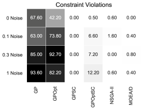
Figure 1: Percentage of infeasible models generated by each algorithm over 30 runs of all instances.

6.7 Results: Sensitivity to Noise

Tables 5 and 6 show the median NMSE of the best solution for each instance out of 30 runs. Table 5 shows results for no noise and $10\%$ noise, Table 6 shows results for $30\%$ and $100\%$ noise.

The result tables are split in two sections. The section on the left side shows the error values of the algorithms without shape constraints. The section on the right side shows results with shape constraints. The best result in each row is highlighted.

Analyzing the tables we notice that algorithms with shape constraints are not better on instances with no or low noise. This is consistent with the finding in [18]. However, here we observe that with increasing noise shape constraints help to improve the results. The row counts where the algorithms with shape constraints are better/equal/worse than without shape constraints are $(2,6,5)$ without noise, $(12,0,1)$ with 10% noise, $(9,0,4)$ with 30% noise, and $(10,0,3)$ with 100% noise.

Table 5: Median NMSE values for test with no noise and 10% noise

		w/o. info			w. info
		GP	GPOpt	PR	GPSC	GPOptSC	SCPR	NSGA-II	MOEA/D
no noise	I.6.20	$0.31$	0.00	$0.01$	$2.25$	0.00	$0.16$	$0.10$	$0.32$
	I.9.18	$0.98$	0.60	$1.05$	$1.12$	$1.21$	$1.20$	$0.81$	$1.20$
	I.15.3x	$0.08$	0.00	$0.06$	$0.09$	$0.01$	$0.08$	$0.03$	$0.03$
	I.30.5	0.00	0.00	$0.14$	$0.15$	0.00	$0.25$	0.00	0.00
	I.32.17	$0.04$	$0.06$	$50.70$	$0.66$	$0.34$	$7.64$	0.02	$0.80$
	I.41.16	0.18	$0.26$	$9.10$	$5.61$	$5.20$	$7.51$	$3.78$	$8.03$
	I.48.20	0.00	0.00	0.00	0.00	0.00	0.00	0.00	0.00
	II.6.15a	$0.46$	0.01	$17.15$	$1.43$	$0.61$	$27.63$	$0.13$	$0.43$
	II.11.27	0.00	0.00	$0.02$	0.00	0.00	$0.02$	0.00	0.00
	II.11.28	0.00	0.00	$0.00$	0.00	0.00	0.00	0.00	0.00
	II.35.21	$0.53$	0.00	$0.96$	$2.96$	$0.46$	$1.45$	$0.75$	$3.90$
	III.9.52	$11.47$	$10.14$	$55.56$	$71.79$	$8.51$	$43.08$	7.41	$41.36$
	III.10.19	$0.29$	0.00	0.00	$0.62$	$0.02$	0.00	$0.07$	$0.74$
noise 10%	I.6.20	$2.00$	$1.83$	$2.73$	$3.30$	1.53	$3.17$	$2.54$	$2.96$
	I.9.18	$2.92$	$5.34$	$6.82$	$2.82$	$3.98$	$4.62$	2.20	$3.42$
	I.15.3x	$1.59$	$2.05$	$3.17$	$1.37$	$1.79$	$5.14$	0.95	$1.38$
	I.30.5	0.13	$0.32$	$4.75$	$0.92$	$1.03$	$2.61$	$0.52$	$0.87$
	I.32.17	$2.56$	$4.45$	$32.48$	$2.57$	$5.15$	$9.29$	1.97	$4.85$
	I.41.16	$3.89$	$5.79$	$23.19$	$5.98$	$7.24$	$12.27$	3.87	$8.17$
	I.48.20	$0.87$	$1.13$	$6.67$	0.31	0.31	$4.11$	0.31	0.31
	II.6.15a	$3.43$	$7.51$	$26.26$	$3.09$	$2.32$	$40.66$	1.32	$7.65$
	II.11.27	$0.72$	$0.60$	$3.30$	$0.71$	$0.64$	$3.30$	0.53	$0.73$
	II.11.28	$0.28$	$0.60$	$0.98$	0.13	0.13	$1.16$	0.13	$0.41$
	II.35.21	$2.33$	$2.14$	$3.60$	$4.07$	$3.93$	$12.36$	1.88	$5.26$
	III.9.52	$15.06$	$11.09$	$59.90$	$78.43$	$31.38$	$53.41$	7.56	$85.22$
	III.10.19	$1.70$	$1.29$	$3.48$	$1.66$	$1.42$	$6.29$	1.22	$1.78$

Table 6: Median NMSE values for test with 30% and 100% noise

		w/o. info			w. info
		GP	GPOpt	PR	GPSC	GPOptSC	SCPR	NSGA-II	MOEA/D
noise 30%	I.6.20	$5.33$	$4.15$	$5.22$	$4.31$	$4.24$	$7.28$	2.61	$3.27$
	I.9.18	$1.89$	$3.42$	$7.63$	$1.65$	$2.28$	$3.78$	1.05	$2.58$
	I.15.3x	$3.71$	$3.54$	1.86	$5.16$	$2.66$	$4.30$	$2.25$	$4.15$
	I.30.5	$2.77$	2.53	$11.52$	$3.34$	$3.71$	$8.89$	$3.24$	$3.32$
	I.32.17	$4.53$	$13.26$	$78.01$	$4.90$	$5.69$	$47.90$	3.33	$5.35$
	I.41.16	$10.00$	$13.08$	$56.95$	$8.50$	$9.81$	$62.72$	4.73	$12.20$
	I.48.20	$1.94$	$2.18$	$5.73$	1.07	1.07	$3.24$	$2.10$	$1.99$
	II.6.15a	$7.66$	$10.32$	$40.73$	$3.13$	$15.07$	$50.17$	2.68	$11.37$
	II.11.27	$6.26$	$6.61$	$26.94$	$3.12$	2.70	$11.47$	$2.76$	$3.01$
	II.11.28	$2.44$	$2.44$	1.48	$1.78$	$1.78$	$1.57$	$1.78$	$2.46$
	II.35.21	$4.76$	$6.14$	$16.05$	$4.43$	$4.08$	$5.07$	3.10	$4.76$
	III.9.52	$39.53$	$16.83$	$56.24$	$74.84$	$39.10$	$52.13$	12.23	$75.67$
	III.10.19	4.24	4.24	$6.42$	$4.68$	$4.76$	$4.33$	$4.79$	$4.69$
noise 100%	I.6.20	$4.28$	$4.31$	$56.27$	$5.67$	$5.82$	$56.26$	4.06	$6.08$
	I.9.18	$9.03$	$19.08$	$9.02$	$9.21$	$18.54$	$28.37$	6.51	$18.91$
	I.15.3x	$6.69$	$12.60$	$12.61$	$7.07$	$7.28$	$12.61$	6.17	$6.81$
	I.30.5	1.97	$11.39$	$15.77$	$6.01$	$8.71$	$4.99$	$6.56$	$5.98$
	I.32.17	$24.76$	$46.56$	$108.27$	$9.59$	$12.31$	$69.67$	7.30	$14.55$
	I.41.16	$27.57$	$55.76$	$102.81$	$23.86$	$27.03$	$102.81$	19.24	$30.77$
	I.48.20	$3.75$	$4.89$	$13.45$	$4.38$	$4.13$	2.59	$4.93$	$4.25$
	II.6.15a	$24.22$	$29.62$	$100.18$	$17.01$	$18.77$	$82.35$	16.59	$21.89$
	II.11.27	2.19	$22.52$	$106.57$	$6.11$	$5.88$	$52.93$	$3.04$	$5.24$
	II.11.28	$2.72$	$2.67$	$23.42$	2.54	$2.59$	$23.42$	$2.61$	$2.64$
	II.35.21	$23.45$	$19.25$	$80.97$	$17.66$	$17.52$	$80.97$	17.10	$18.34$
	III.9.52	$65.65$	$45.94$	$100.21$	$82.67$	$78.29$	$100.21$	26.62	$84.44$
	III.10.19	$9.20$	5.41	$53.01$	$7.01$	$11.64$	$12.03$	$7.75$	$7.63$

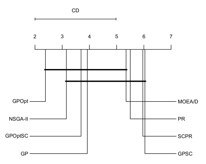
(a) CD plot on noise level 0%

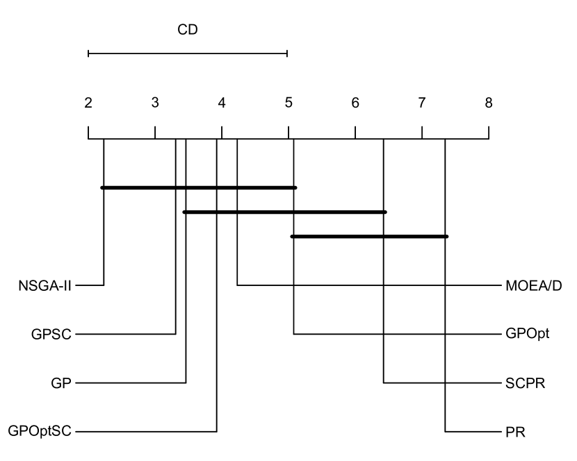
(b) CD plot on noise level 100%

Figure 2: Critical difference plots in-domain performance

The critical difference (CD) plots in Figure 2 show the average rank of the different algorithms. As we can see in Figure 2(a) GPOpt has the best overall rank and is significantly better than PR, SCPR and GPSC. All other algorithms do not have a significant difference to each other and GPSC performs worst without noise. In Figure 2(b) the CD plot for highest noise level shows, that the algorithms with shape constraints rank better than for the instances without noise. For the highest noise level NSGA-II performs best overall and GPSC has the second best rank.

PR and SCPR do not perform well compared to the evolutionary algorithms. The CD plots in Figure 2 show that PR and SCPR rank significant worse than the best algorithms. This is in contrast to [18] where we observed that SCPR produced the best results for no noise or low-noise problem instances. The reason for this difference is that in the new experiments we tuned hyper-parameters for the evolutionary algorithms using a grid search and achieved better prediction errors. At the same time hyper-parameter selection for PR and SCPR was changed to improve results for high-noise problem instances which lead to increased prediction errors for the low noise experiments.

7 Analysis of Out-of-domain Performance

The results above show that shape constraints can help to find SR models that conform to expected behavior especially for high noise settings. However, we did not detect a significant difference to the best algorithms without shape constraints. Shape constraints may also improve the prediction error for extrapolation when new observations lie outside of the domain of the training error. In this second set of experiments we try to find evidence for this hypothesis.

7.1 Problem instances

For analysing the out-of-domain prediction errors, we use three additional problem instances: Kotanchek and UnwrappedBall from [37], and a problem instance from [26] in the following called Pagie. The first two problem instances are chosen because they were also used for analysing extrapolation capabilities of SR in [37] and additionally because they are monotonic in large subsets of the input space.

Table 7 shows the generating expressions for the three additional problem instances, Table 8 shows the definition of the input space and the shape constraints. For these three instances we use different constraints on non-overlapping subspaces of the input space whereby we split the input spaces at the extrema of the three functions which are located at $(0,0)$ for Pagie, $(1,2.5)$ for Kotanchek and $(3,3,3,3,3)$ for UnwrappedBall.

For the extrapolation instances, we generate samples within the input domain until the training, validation and test partitions had $100$ samples each. To split the data into training and test sets we use the condition that all samples that lie in the first $x\%$ or the last $x\%$ of the domain range, are assigned to the test set. For the Feynman, Kotanchek and UnwrappedBall instances we use $10\%$ for the test set and for Pagie we increase the fraction to $30\%$. This procedure ensures that the test samples are located in the outer hull of the data set. We add noise to the target values in the training sets as described above.

Table 7: Expressions for the additional problem instances

Instance	Expression
Pagie [26]	$\frac{1}{1+{{x}^{-4}}}+\frac{1}{1+{{y}^{-4}}}$
Kotanchek [37]	$\frac{\operatorname{exp}\left((x1-1)^{2}\right)}{1.2+(x2-2.5)^{2}}$
UnwrappedBall [37]	$\frac{10}{5+\sum_{n=1}^{5}(x_{i}-3)^{2}}$

Table 8: Shape constraints used for additional problem instances taken from [26] and [37]

Instance	Input space	Constraints
Pagie	$\left(x,y\right)\in[-5\ldots 5]^{2}$	$f(x,y)\in[0..2]$
		$\frac{\partial}{\partial x}f(x,y)\leq 0,x<0$
		$\frac{\partial}{\partial x}f(x,y)\geq 0,x>0$
		$\frac{\partial}{\partial y}f(x,y)\leq 0,y<0$
		$\frac{\partial}{\partial y}f(x,y)\geq 0,y>0$
Kotanchek	$\left(x_{1},x_{2}\right)\in[-0.2\ldots 4.2]^{2}$	$f(x_{1},x_{2})\in[0\ldots 1]$
		$\frac{\partial}{\partial x_{1}}f(x_{1},x_{2})\geq 0,x_{1}<1$
		$\frac{\partial}{\partial x_{1}}f(x_{1},x_{2})\leq 0,x_{1}>1$
		$\frac{\partial}{\partial x_{2}}f(x_{1},x_{2})\geq 0,x_{2}<2.5$
		$\frac{\partial}{\partial x_{2}}f(x_{1},x_{2})\leq 0,x_{2}>2.5$
UnwrappedBall	$\left(x_{1},x_{2},x_{3},x_{4},x_{5}\right)$	$f(\textbf{x})\in[0\ldots 2]$
	$\in[-0.25\ldots 6.35]^{5}$	$\forall_{i\in\{1\ldots 5\}}:$
		$\frac{\partial}{\partial x_{i}}f(\textbf{x})\geq 0,x_{i}<3$
		$\frac{\partial}{\partial x_{i}}f(\textbf{x})\leq 0,x_{i}>3$

7.2 Experimental setup

We use the same algorithms and parameter settings as for the first set of experiments. We re-run the grid-search for the best configuration because in this set of experiments the input space for the training set is smaller than before and may have an effect on the optimal parameter settings. Again 30 independent runs are executed for each problem instance using the best settings from the grid-search.

7.3 Results: Effect on Extrapolation

Figures 3 and 4 show the effect of shape constraints using the Pagie problem as an example. The four panels show partial dependence plots for GP and GPOpt and their extensions with shape constraints (GPSC and GPOptSC). Each partial dependence plot shows the outputs of models found in 30 independent runs over x (with $y=0$) and over y (with $x=0$).

Figure 3 shows the results without noise, here GPOpt shows best performance as it identified the optimal solution in all runs and correspondingly the extrapolation is perfect even without shape constraints. GP produces the worst models whereby the algorithm has high variance especially for the extrapolation region. The introduction of shape constraints into GP significantly improves the models and produces better predictions for the extrapolation region. However, for GPOptSC the results are slightly worse which indicates that the introduction of shape constraints makes it harder to identify optimal solutions.

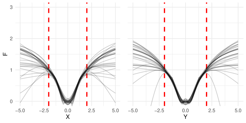
(a) GP

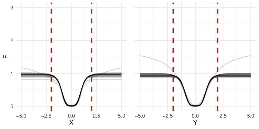
(b) GPSC

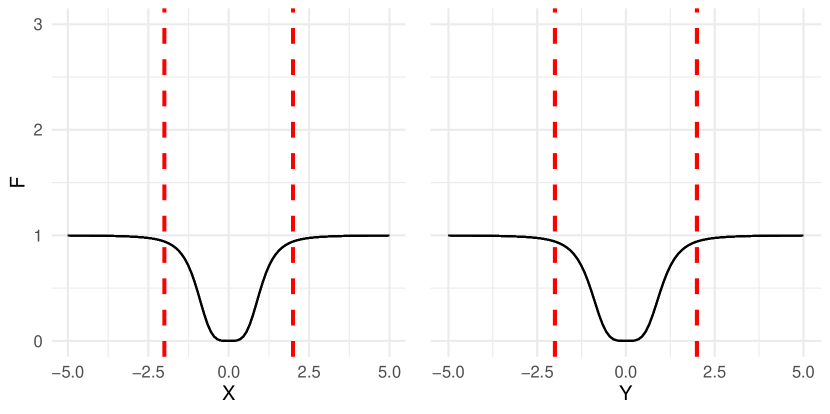
(c) GPOpt

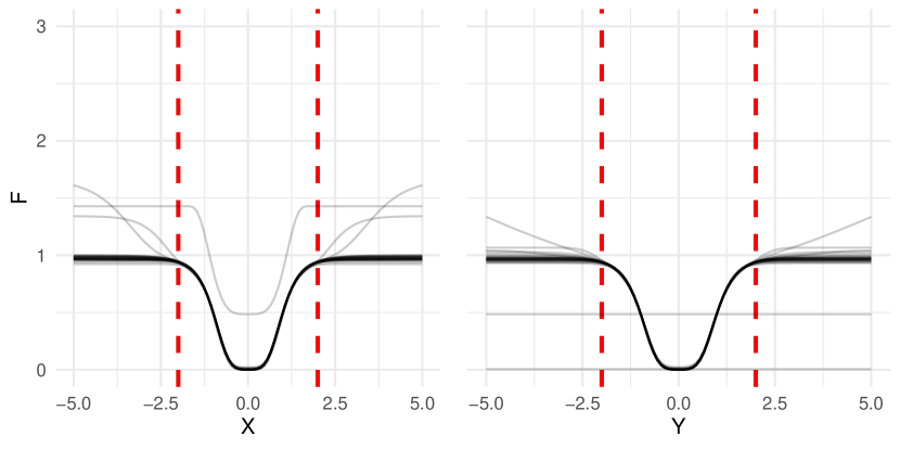
(d) GPOptSc

Figure 3: Partial dependence plots for the 30 models identified for the Pagie problem without noise.

Figure 4 shows the same plots with $10\%$ noise. GP again produces the worst models and has high variance in the extrapolation region. GPSC is again much better and produces very similar results as without noise. With noise, GPOpt is not able to identify the optimal solution anymore and tends to overfit, leading to extreme extrapolation (especially over input variable X). GPOptSC is again much better than GPOpt and similar to GPSC.

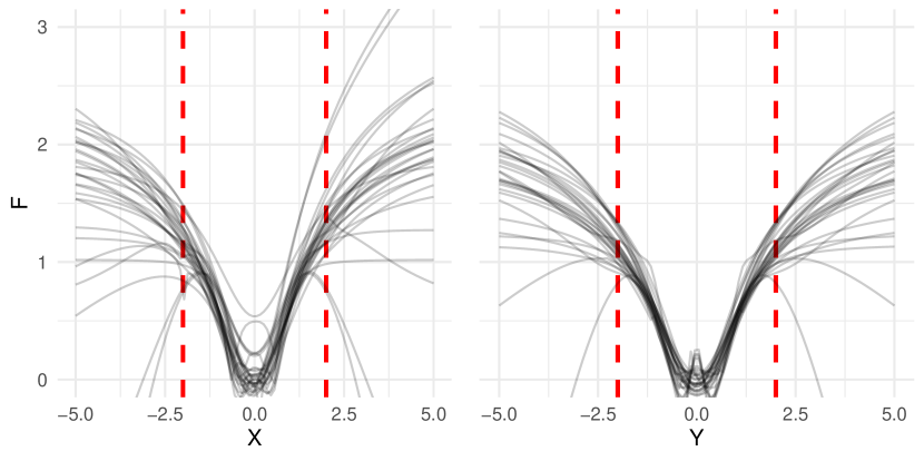
(a) GP

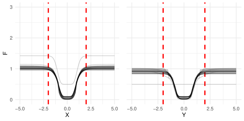
(b) GPSC

(c) GPOpt

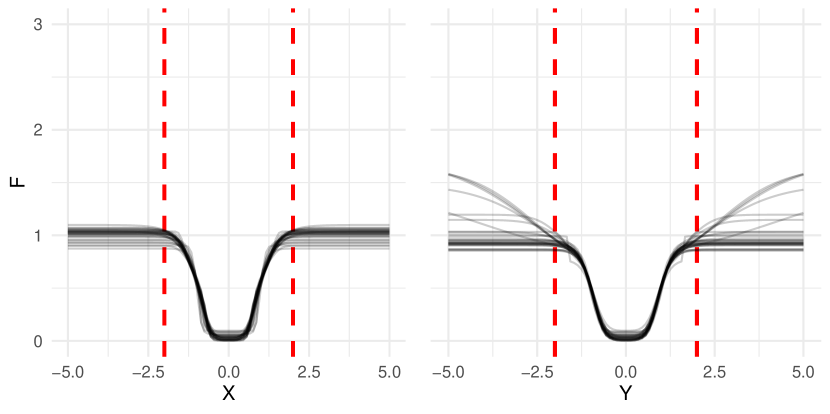
(d) GPOptSc

Figure 4: Partial dependence plots for the models identified for the Pagie problem with 10% noise.

These results highlight that shape constraints can improve prediction errors for noisy problems especially for extrapolation and that overfitting can be reduced. However, when it is possible to reliably find the optimal solution then shape constraints may hamper the search.

Figure 5 shows Box plots over all extrapolation instances with 100% noise. On the y-axis the NMSE is plotted and on the x-axis the different algorithms are plotted. For better visualization we have limited the range of the y-axis for some plots and cut off a few outliers. We can also see that there is no algorithm which performs best over all instances.

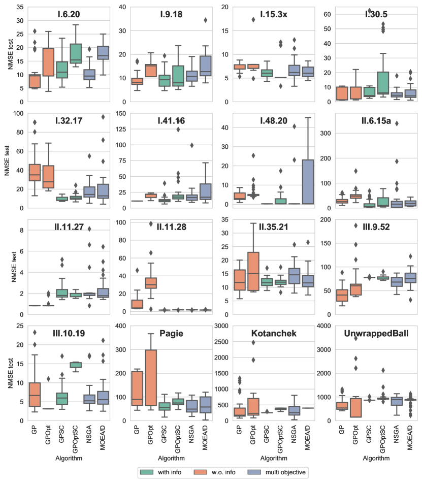
Figure 5: NMSE of extrapolation datasets with high noise. The optimal achievable NMSE is zero. Following outliers are cut off: I.6.20: GPOpt(1); I.15.3x: NSGA-II(1); I.30.5: NSGA-II(1); I.32.17: NSGA-II(1); I.41.16: GPOptSC(1); II.6.15a: NSGA-II(1), GPOptSC(2); II.35.21: NSGA-II(1); III.9.52: GP(3); Pagie: GPOpt(2); Kotanchek: GPOptSC(4), GPOpt(2); UnwrappedBall: GPOptSC(1), GPOpt(2)

Table 9 shows the NMSE over all instances on the extrapolation dataset for the no noise and $10\%$ noise level. Table 10 shows the high noise levels $30\%$ and $100\%$. Each of the tables is separated into two section. The left section shows the error values of the algorithms without using shape constraints and the right section shows the algorithms with shape constraints. The best result for each row is highlighted.

Table 9: Median NMSE values for extrapolation datasets with no noise and 10% noise

		w/o. info			w. info
		GP	GPOpt	PR	GPSC	GPOptSc	SCPR	NSGA-II	MOEA/D
no noise	I.6.20	$1.30$	0.00	$0.08$	$7.20$	$0.32$	$0.04$	$3.49$	$11.26$
	I.9.18	$0.91$	0.50	$0.81$	$17.78$	$0.79$	$0.62$	$1.68$	$1.54$
	I.15.3x	$0.18$	0.00	$0.04$	$0.27$	$0.03$	$0.04$	$0.27$	$0.42$
	I.30.5	$0.01$	0.00	$0.41$	$0.39$	$0.05$	$0.53$	$0.81$	$1.32$
	I.32.17	$0.13$	0.05	$12.79$	$0.74$	$0.50$	$7.14$	$1.62$	$1.52$
	I.41.16	$1.44$	0.25	$1.94$	$7.74$	$4.58$	$2.78$	$6.23$	$6.94$
	I.48.20	0.00	0.00	0.00	0.00	0.00	0.00	0.00	0.00
	II.6.15a	$1.07$	0.19	$27.03$	$5.19$	$1.73$	$14.26$	$2.11$	$7.75$
	II.11.27	0.00	0.00	0.00	0.00	0.00	0.00	0.00	0.00
	II.11.28	0.00	0.00	0.00	0.00	0.00	0.00	0.00	0.00
	II.35.21	$3.10$	0.01	$1.63$	$5.44$	$1.44$	$1.28$	$4.45$	$7.18$
	III.9.52	$7.34$	0.48	$194.32$	$44.67$	$22.25$	$194.37$	$50.40$	$61.42$
	III.10.19	$0.38$	0.00	0.00	$0.71$	$0.02$	0.00	$0.76$	$0.75$
	Pagie	$47.49$	0.00	$4.62e8$	$3.91$	$1.06$	$64.36$	$3.01$	$3.75$
	Kotanchek	$28.47$	0.00	$2.72e5$	$265.58$	$266.22$	$6.60$	$266.22$	$266.22$
	UnwrappedBall	$185.11$	25.02	$919.27$	$804.25$	$895.51$	$775.13$	$805.21$	$807.69$
noise 10%	I.6.20	$2.17$	1.54	$4.81$	$5.75$	$6.29$	$3.85$	$4.23$	$12.10$
	I.9.18	$28.24$	$26.92$	$9.12$	$17.78$	$13.85$	$6.08$	2.73	$3.40$
	I.15.3x	$1.49$	1.47	$1.99$	$1.50$	$1.49$	$1.99$	$1.49$	$1.58$
	I.30.5	0.31	$0.57$	$8.79$	$1.53$	$1.40$	$7.04$	$0.99$	$1.29$
	I.32.17	1.85	$5.36$	$29.39$	$3.39$	$4.17$	$17.19$	$3.07$	$3.22$
	I.41.16	3.62	$9.04$	$25.61$	$5.32$	$7.24$	$5.64$	$5.53$	$7.41$
	I.48.20	$0.32$	$1.35$	$2.63$	0.13	0.13	$2.00$	$2.00$	0.13
	II.6.15a	1.99	$8.22$	$62.56$	$4.04$	$5.02$	$40.89$	$2.74$	$7.45$
	II.11.27	$0.19$	$0.61$	$4.89$	0.10	$0.20$	$2.41$	$0.11$	$0.11$
	II.11.28	$0.92$	$1.97$	$2.72$	0.02	0.02	$3.44$	0.02	0.02
	II.35.21	5.42	$5.80$	$9.10$	$9.11$	$5.80$	$7.51$	$7.83$	$9.87$
	III.9.52	8.23	$9.58$	$89.44$	$50.50$	$22.70$	$75.46$	$33.08$	$62.23$
	III.10.19	$0.92$	$0.98$	$2.05$	$0.83$	0.86	$2.06$	$0.87$	$0.87$
	Pagie	$79.11$	$32.41$	$3.88e5$	$20.44$	$22.52$	$63.47$	18.63	$20.01$
	Kotanchek	$38.63$	$15.19$	$91.83$	$265.25$	$265.25$	14.46	$265.25$	$265.25$
	UnwrappedBall	$219.3$	78.2	$105.99$	$836.42$	$919.98$	$561.10$	$821.39$	$843.12$

Table 10: Median NMSE values for extrapolation datasets with 30% noise and 100% noise

		w/o. info			w. info
		GP	GPOpt	PR	GPSC	GPOptSC	SCPR	NSGA-II	MOEA/D
noise 30%	I.6.20	8.95	$9.56$	$13.41$	$10.42$	$10.65$	$12.68$	$10.03$	$12.23$
	I.9.18	$29.23$	$14.32$	$11.02$	$17.95$	$15.58$	$8.95$	5.95	$6.16$
	I.15.3x	$5.64$	$5.00$	1.44	$4.39$	$1.79$	1.44	$2.88$	$3.25$
	I.30.5	1.20	$5.72$	$20.36$	$3.84$	$5.31$	$12.29$	$4.14$	$3.33$
	I.32.17	5.45	$20.88$	$46.22$	$7.91$	$7.64$	$24.09$	$8.47$	$6.44$
	I.41.16	2.94	$14.21$	$29.83$	$7.69$	$11.61$	$12.31$	$9.87$	$10.07$
	I.48.20	$2.97$	$3.57$	$16.66$	0.81	0.81	$16.32$	0.81	0.81
	II.6.15a	$12.60$	$14.71$	$60.99$	$5.32$	$13.63$	$48.23$	2.87	$6.63$
	II.11.27	1.94	1.94	$6.89$	$2.10$	$2.05$	$5.39$	$2.19$	$1.96$
	II.11.28	$2.22$	$4.08$	$3.68$	$0.46$	$0.40$	$4.10$	0.37	0.37
	II.35.21	8.34	$9.69$	$10.18$	$9.41$	$9.21$	$14.86$	$9.15$	$9.33$
	III.9.52	13.25	$15.77$	$67.50$	$51.96$	$42.88$	$46.88$	$54.98$	$69.48$
	III.10.19	$6.12$	3.81	$8.72$	$4.97$	$6.01$	$3.47$	$4.88$	$5.20$
	Pagie	$377.15$	$90.07$	$2.44e5$	9.44	$13.92$	$60.48$	$9.56$	$10.21$
	Kotanchek	$96.11$	12.39	$608.18$	$287.85$	$287.85$	$16.71$	$287.85$	$287.85$
	UnwrappedBall	$385.89$	82.75	$208.41$	$724.45$	$835.37$	$431.90$	$821.01$	$825.21$
noise 100%	I.6.20	$9.59$	$19.71$	$30.36$	$10.95$	$15.45$	$30.36$	8.87	$17.02$
	I.9.18	$14.13$	$15.16$	$21.23$	$13.19$	$13.79$	$19.34$	12.69	$12.72$
	I.15.3x	$6.91$	$7.06$	$48.39$	$6.05$	$5.13$	$48.39$	5.41	$6.03$
	I.30.5	1.47	$2.04$	$40.17$	$4.35$	$6.15$	$52.04$	$4.66$	$4.11$
	I.32.17	$15.89$	$27.8$	$100.01$	8.38	$10.61$	$59.07$	$11.47$	$12.90$
	I.41.16	11.27	$22.01$	$58.91$	$12.05$	$17.46$	$28.68$	$16.23$	$16.12$
	I.48.20	$2.95$	$4.64$	$14.74$	0.25	0.25	$27.65$	0.25	0.25
	II.6.15a	$26.14$	$48.11$	$85.30$	$6.62$	$10.61$	$87.42$	5.40	$18.05$
	II.11.27	0.83	0.83	$26.93$	$1.80$	$1.99$	$21.54$	$1.79$	$1.78$
	II.11.28	$4.06$	$30.05$	$24.77$	1.66	$1.97$	$4.58$	$1.99$	1.66
	II.35.21	$11.78$	$15.08$	$19.09$	$11.72$	$11.89$	$12.30$	11.04	$11.81$
	III.9.52	40.90	$60.28$	$78.22$	$77.72$	$75.60$	$73.26$	$73.01$	$75.81$
	III.10.19	$6.67$	3.14	$10.45$	$5.97$	$14.04$	$10.45$	$6.18$	$7.14$
	Pagie	$90.07$	$63.33$	$1.06e5$	$55.66$	$74.72$	$55.84$	54.21	$55.12$
	Kotanchek	$174.67$	$234.35$	$457$	$252.06$	$387.16$	40.06	$387.16$	$387.16$
	UnwrappedBall	$539.40$	153.52	$287.91$	$864.29$	$934.47$	$1016.75$	$854.92$	$867.21$

The number of rows where the algorithms with shape constraints are better/equal/worse than without shape constraints are: $(0,4,12)$ without noise, $(7,0,9)$ with 10% noise, $(5,1,10)$ with 30% noise, and $(10,0,6)$ with 100% noise. Without noise the results are again worse with shape constraints. For the noisy problems the disadvantage is smaller, but the results do not show that shape constraints improve the results as strongly as observed for the in-domain problem instances.

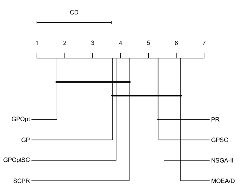
(a) CD plot on noise level 0%

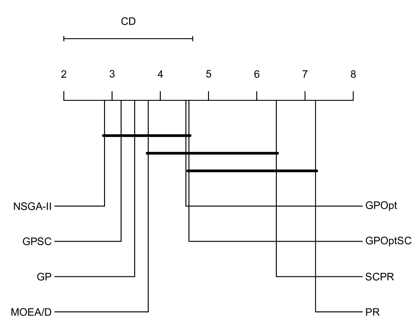
(b) CD plot on noise level 100%

Figure 6: Critical difference plots for out-of-sample (extrapolation) performance

Figure 6(a) shows that GPOpt has the best rank overall and has significantly better ranking than PR, GPSC, NSGA-II and MOEA/D. The CD plot for 100% noise in Figure 6(b) shows that again NSGA-II has the overall best rank and is significantly better than PR and SCPR. The CD plots for in-sample and out-of-sample performance are similar.

8 Discussion

NSGA-II produced on average the best results for the highest noise, but we found no statistically significant difference between multi-objective algorithms and the best single-objective algorithm. However, multi-objective algorithms offer the possibility to handle each constraint violation separately by using different solutions from the resulting Pareto front. For the comparison with the single-objective results, we took the solution with best NMSE from the Pareto front.

We did not find a significant difference between MOEA/D and NSGA-II. MOEA/D may have an advantage with more constraints but we have not analyzed this in detail so far. SPEA2 and NSGA-III are potentially also interesting alternatives that could be tried to improve SCSR results.

Inclusion of shape constraints has a small effect on the runtime. Checking constraint bounds using interval arithmetic is only slightly more costly than evaluation of the model for one data point. The calculation of partial derivatives for each solution candidate is an additional computational burden which depends mainly on the size of candidate models. We only consider first or second derivatives, so the additional computational effort is rather small.

Our experiments are focused on synthetic datasets where the underlying model can be expressed as a short mathematical formula. All problem instances that we have used have low dimensionality. We do not know yet how well SCSR works for high-dimensional problem instances.

We have so far only analyzed a pessimistic approach because we believe it scales better to high-dimensional problems. However, the problem instances from the Feynman Symbolic Regression Database are all low-dimensional. For these models an optimistic approach based on sampling is also computationally feasible. We have not yet compared the optimistic approach with IA and leave this for future work.

9 Conclusion

Our results show that including shape constraints into genetic programming via interval arithmetic leads to solutions with higher prediction error for low-noise settings. We have already observed this in our previous experiments [18]. The new results including other problem instances, and multi-objective algorithms again support this conclusion. With shape constraints we found better models for the higher noise levels, but we found no statistically significant difference to single-objective genetic programming without shape constraints.

Multi-objective algorithms for shape-constrained symbolic regression which do not reject infeasible solutions immediately produce similar results as single-objective algorithms. On average we found the best results with NSGA-II but the difference to the other shape-constrained algorithms was small. We found no significant difference between overall rankings of NSGA-II and the best algorithm without constraints.

The results for in-domain predictions and out-of-domain predictions are similar. We did not find convincing evidence for our hypothesis that shape constraints are more helpful for extrapolation (out-of-domain predictions) in general. However, we could show for a single problem instance that shape constraints produced much better out-of-domain predictions. The effect is very problem specific.

For the selected problem instances the evolutionary algorithms for shape-constrained symbolic regression produced better models on average than shape-constrained polynomial regression which is a deterministic approach with a strong mathematical background. However, this requires a computationally costly grid-search to optimize hyper-parameters for each problem instance.

Still an open topic are the overly wide bounds produced by interval arithmetic. Alternative methods which produce tighter bounds could improve evolutionary dynamics and better prediction results. Another interesting idea for future work is to limit the functional complexity of regression models via shape constraints to limit the maximum slope or curvature of models.

References

- Abu-Mostafa [1992] Abu-Mostafa, Y., 1992. A method for learning from hints. Advances in Neural Information Processing Systems 5, 73–80.