Uncertainty Relations for the Relativistic Jackiw-Nair Anyon:
A First Principles Derivation

Abstract

joydeepmjh@gmail.com (Joydeep Majhi), subirghosh20@gmail.com (Subir Ghosh)

In this paper we have explicitly computed the $position-position$ and $position-momentum$ (Heisenberg) Uncertainty Relations for the model of relativistic particles with arbitrary spin, proposed by Jackiw and Nair jn as a model for Anyon, in a purely quantum mechanical framework. This supports (via Schwarz inequality) the conjecture that anyons live in a 2-dimensional noncommutative space. We have computed the non-trivial uncertainty relation between anyon coordinates, ${\sqrt{\Delta x^{2}\Delta y^{2}}}=\hbar\bar{\Theta}_{xy}$, using the recently constructed anyon wave function jan , in the framework of bel . We also compute the Heisenberg (position-momentum) uncertainty relation for anyons. Lastly we show that the identical formalism when applied to electrons, yield a trivial position uncertainty relation, consistent with their living in a 3-dimensional commutative space.

Introduction: Consider $x,y$ to be the spatial coordinates for excitations in a $2+1$-dimensional field theoretic model, proposed by Jackiw and Nair jn (see also p248 ), that describes relativistic particles of arbitrary spin, purportedly referred to as Anyons lm ; wan1 ; wan2 , (although its arbitrary statistics was not shown). In this paper we explicitly show, in a quantum mechanical framework, that the position uncertainty relation ${\sqrt{\Delta x^{2}\Delta y^{2}}}=\bar{\Theta}_{xy}$ for these anyons has a non-zero lower bound for $\bar{\Theta}_{xy}$, where ${\sqrt{\Delta A^{2}}}$ is the uncertainty (dispersion or fluctuation from the mean value i.e. standard deviation) of a generic hermitian operator $A$. Our result agrees with the commonly used assumption that anyons live in Non-Commutative (NC) space. The Schwarz inequality

$${\sqrt{\Delta A^{2}~{}\Delta B^{2}}}\geq\frac{1}{2}<[A,B]>,$$ (1)

if considered for $x,y$, indicates $<[x,y]>\neq 0$. An interesting observation is that $\bar{\Theta}_{xy}$ is the minimum effective spatial area occupied by an anyon. We tentatively claim the $(length)^{2}$-dimensional NC-parameter $\bar{\Theta}_{xy}$ to be a new physical constant. We also compute the Heisenberg Uncertainty Relation (HUR) for anyon ${\sqrt{\Delta r^{2}\Delta p^{2}}}=\hbar$ where $r={\sqrt{x^{2}+y^{2}}},~{}p={\sqrt{p_{x}^{2}+p_{y}^{2}}}$. These results for anyons are new.

In deriving the above, we have used a technique, recently formulated by Bialynicki-Birula and Bialynicka-Birula bel , who compute HUR for free electrons, using spinor wave functions (see also bph1 ; bph2 ; bbos ). We follow the same procedure to derive the above uncertainty relations for anyons, making use of the recently constructed anyon wavefunction from a work involving the present authors jan .

Since our demonstration of the counter intuitive non-zero result $\bar{\Theta}_{xy}$ for anyons is new, we need to show that the result is not a spurious artifact of our formalism. Thus we use the same formalism bel to calculate spatial uncertainty relation for conventional $3+1$-dimensional electrons; this turns out to be zero (as expected) thus establishing robustness of the formalism.

It is to be noted that noncommutativity of $x,y$ and non-zero $\bar{\Theta}_{xy}$ are two completely different issues and here we are directly concerned only with the latter. We stress that possible noncommutative nature of the $x-y$-plane of anyon does not play any role in our study. In fact our result of non-zero $\bar{\Theta}_{xy}$ is (possibly a necessary but) not a sufficient condition condition for noncommutative $x-y$; proving noncommutativity is beyond the scope of our work. It needs to be duly emphasized that the present analysis is done purely in a quantum mechanical framework using anyon wave functions in calculating expectation values $<A>$ because so far, in modelling anyons, an NC algebra (or non-canonical algebra) between anyon dynamical variables were simply posited in a semi-classical formalism. In some variants a generalized (spinning) point particle model was constructed which had constraints that yielded Dirac brackets, to be identified with the NC algebra (see for example spinan ; ghosh ; duval ; nair ; chou ; ghosh2 ; c11 ). The NC algebra was geared to generate the arbitrary anyon spin. A non-relativistic limit of the Jackiw-Nair anyon, as suggested in jn2 , also yields a non-commutative spatial algebra, as proved in h595 . In the present work we have provided a totally quantum mechanical treatment for the anyon, based on the Jackiw-Nair anyon model.

The impact of anyons in theoretical and applied physics is easily established from its ubiquitous role in High Energy (via Chern-Simons theory aa01 ; aa02 ) to Condensed Matter (quantum Hall effect aa1 , high $T_{c}$ superconductivity aa2 ) to the exciting arena of non-Abelian anyons (in fault tolerant quantum computation aa3 ; aa4 ). The posssibility of noncommutative space and its effect on modern physics can be seen in ncrev ; szabo ; ban . Thus a thorough understanding of anyon theory and its living in a noncommutative space is necessary.

The quantum mechanical Jackiw-Nair model of jn was extended in jan to the full construction of anyon wave function. The scheme of bel is well-suited for our purpose since the Jackiw-Nair equation for anyon is structurally similar to the Dirac equation for electron, both being first order in derivatives. Crucial difference in solutions is that anyon wave function is an infinite component one although constraints are imposed to reduce it to a single polarization jn ; jan . Apart from the anyonic position UR we also compute;
(i) ${\sqrt{\Delta r^{2}\Delta p^{2}}}=\hbar$ HUR for anyons and (ii) show in the framework of bel that $\Delta x^{2}\Delta y^{2}=0$ for electron in $3+1$-dimensions which is indeed reassuring.

Outline of the formalism:

The probability densities in position and momentum space, for a generic system, are defined as $\rho_{r}(\boldsymbol{r})=|\psi(\boldsymbol{r})|^{2}=\sum_{\beta}|\psi_{\beta}(\boldsymbol{r})|^{2},~{}\rho_{p}(\boldsymbol{p})=|\tilde{\psi}(\boldsymbol{p})|^{2}=\sum_{\beta}|\tilde{\psi}_{\beta}(\boldsymbol{p})|^{2}$, where $\tilde{\psi}(p)$ is the Fourier transform of $\psi(r)$ and $\psi_{\beta}$ are the components of the column vector $\psi$. Now $\psi_{\beta}(\boldsymbol{r},t)$ can be expressed as

$$\psi_{\beta}(\boldsymbol{r},t)=\int\frac{d^{2}p}{2\pi}~{}F_{\beta}(\boldsymbol{p})v_{\beta}(\boldsymbol{p})e^{i(\boldsymbol{p}.\boldsymbol{r}-iE_{p}t)}$$ (2)

where $F_{\beta}(\boldsymbol{p})$ is orthonormalized free particle solution and $v_{\beta}(\boldsymbol{p})$ is an arbitrary function with $\beta$ referring to components of the column vector.

The standard expressions for the dispersions $\Delta r^{2}$ and $\Delta p^{2}$ in terms of the probability densities in position and momentum space

$$\Delta r^{2}=\frac{1}{N^{2}}\int d^{3}r(\vec{r}-\langle\boldsymbol{r}\rangle)^{2}\rho_{r}(\boldsymbol{r})$$ (3)

$$\Delta p^{2}=\frac{1}{N^{2}}\int d^{3}p(\vec{p}-\langle\boldsymbol{p}\rangle)^{2}\rho_{p}(\boldsymbol{p})$$ (4)

are calculated, where $N^{2}$ is the normalization constant,

$$N^{2}=\int d^{3}r~{}\rho_{r}(\boldsymbol{r})=\int d^{3}p~{}\rho_{p}(\boldsymbol{p}).$$ (5)

Uncertainty relations are always formulated at a fixed time. Without loss of generality, $<\boldsymbol{r}>,~{}<\boldsymbol{p}>$ can be dropped from (3,4) bel . In terms of the wavefunctions, we find

$$N^{2}=\int d^{3}p\mid v(\boldsymbol{p})\mid^{2}$$ (6)

where the function $v(\boldsymbol{p})$ of momentum variable represents the independent degrees of freedom of an anyon moving in free space.

$\Delta p^{2}$ is trivially given by

$$\Delta p^{2}=\frac{1}{N^{2}}\int d^{3}p~{}\boldsymbol{p}^{2}\mid v(\boldsymbol{p})\mid^{2}$$ (7)

whereas $\Delta r^{2}$ can be found by using the following identity bel ,

$$\boldsymbol{r}\psi_{\alpha}(\boldsymbol{r})=\int\frac{d^{3}p}{(2\pi)^{3/2}}i\boldsymbol{\nabla}_{p}(F_{\alpha}v(\boldsymbol{p}))e^{i\boldsymbol{p}\cdot\boldsymbol{r}},$$ (8)

using (2) with $v(\boldsymbol{p})$ being an arbitrary weight function as mentioned above.

Anyon wavefunction: Let us start with the anyon wave function for an anyon of arbitrary spin $s=1-\lambda$. The dynamical equation for a spin one particle in $2+1$-dimension) in co-ordinate and momentum space $(i\partial_{a}=p_{a})$ is given by jn

$$\partial_{a}\epsilon^{abc}F_{c}\pm mF^{b}=0;~{}~{}~{}(\boldsymbol{p}\cdot\boldsymbol{j})^{a}_{b}F^{b}+msF^{a}=0$$ (9)

with $\boldsymbol{j}$ being the angular momentum operator and m is the mass term. If $\boldsymbol{J}$ is the total spin contribution to the Lorentz generators $\boldsymbol{K}$, then $\boldsymbol{J}=\boldsymbol{K}+\boldsymbol{j}$.

The solution of the three vector $F^{a}$, $a=1,2,3$ in the Minkowski metric $\eta_{\mu\nu}=\textrm{diag}(1,-1,-1)$ is given by

$$F^{a}(p)=\frac{m}{\sqrt{2}E}\left[\begin{bmatrix}0\\ 1\\ i\end{bmatrix}+\frac{p^{x}+ip^{y}}{m(E+m)}\begin{bmatrix}E+m\\ p^{x}\\ p^{y}\end{bmatrix}\right].$$ (10)

This construction has been extended in an elegant way to the Jackiw-Nair anyon equation jn to describe an anyon of arbitrary spin $s=1-\lambda$, whose momentum space dynamics is given by,

$$P.(K+j)_{an\hskip 2.84544pta^{\prime}n^{\prime}}f^{\lambda,a^{\prime}}_{n^{\prime}}+ms{f}^{\lambda}_{an}=0,~{}~{}(D_{a}f^{\lambda,a})_{n}=0,$$ (11)

($D^{a}_{nn^{\prime}}=\epsilon^{a}_{~{}bc}P^{b}K^{c}_{nn^{\prime}}$) where the second equation is the subsidiary (constraint) relation and $n$ runs from 0 to $\infty$. For $\lambda=0$ the anyon reduces to spin one model discussed earlier. The notation and other details can be found in jan (see also jn ). $K^{a}$ are the Lorentz generators with action defined as

$$K^{0}{f}^{\lambda+}_{n}F^{a} =(\lambda+n){f}^{\lambda+}_{n}F^{a}$$ (12)

$$K^{+}{f}^{\lambda+}_{n}F^{a} =\sqrt{(2\lambda+n)(n+1)}{f}^{\lambda+}_{n+1}F^{a}$$

$$K^{-}{f}^{\lambda+}_{n}F^{a} =\sqrt{(2\lambda+n-1)n}{f}^{\lambda+}_{n-1}F^{a}$$

where ”$+$” superscript denotes representations bounded below. There is an analogous bounded above representation and $K^{\pm}=K^{x}\mp iK^{y}$ jn . Thus explicit form of the free anyon solution, ($\infty\geq n\geq 0$) is given by jan

$$f_{n}^{\lambda,a+}= \left(\frac{2m}{E+m}\right)^{\lambda}\sqrt{\frac{\Gamma(2\lambda+n)}{n!\Gamma(2\lambda)}}\left(\frac{p^{x}+ip^{y}}{E+m}\right)^{n}$$ (13)

$$\times F^{a}(p)e^{-ipx}$$

where $F^{a}(p)$ is same as the spin-$1$ case defined in (10).

Before proceeding further let us ensure: (i) The probability distribution thus generated is conserved; (ii) The Lorentz generators defined earlier are self-adjoint. Complications can stem from the sum over index $n$ running from $zero$ to $infinity$ and possible appearance of null or negative norm states. These issues are addressed in val in detail. Furthermore, in val an alternative and more compact anyon model was proposed where, the spin one base used here jn ; jan , was replaced by a Majorana-Dirac spin $1/2$ base.

(i) Anyon current conservation: We will explicitly derive the conservation law for probability current $\partial^{\mu}j_{\mu}^{(s=1-\lambda)}=0$, where $j_{0}^{s}$ denotes the probability density (computational steps are provided in Supplemental Material of jan ). Using explicit form of Anyon wave function (13) a long calculation yields jan ,

$$\partial^{0}\sum_{n=0}^{\infty}\left[\left(f_{n}^{0\dagger}f_{n}^{0}+f_{n}^{x\dagger}f_{n}^{x}+f_{n}^{y\dagger}f_{n}^{y}\right)\right.$$

$$-i\left(f_{n}^{y\dagger}K_{nn^{\prime}}^{0}f_{n^{\prime}}^{x}-f_{n}^{x\dagger}K_{nn^{\prime}}^{0}f_{n^{\prime}}^{y}\right)-\partial^{x}\sum_{n=0}^{\infty}\left[\left(f_{n}^{0\dagger}f_{n}^{x}+f_{n}^{x\dagger}f_{n}^{0}\right)\right.$$

$$\left.-i\left(f_{n}^{y\dagger}K_{nn^{\prime}}^{x}f_{n^{\prime}}^{x}-f_{n}^{x\dagger}K_{nn^{\prime}}^{x}f_{n^{\prime}}^{y}\right)\right]-\partial^{y}\sum_{n=0}^{\infty}\left[\left(f_{n}^{0\dagger}f_{n}^{y}+f_{n}^{y\dagger}f_{n}^{0}\right)\right.$$

$$\left.-i\left(f_{n}^{y\dagger}K_{nn^{\prime}}^{y}f_{n^{\prime}}^{x}-f_{n}^{x\dagger}K_{nn^{\prime}}^{y}f_{n^{\prime}}^{y}\right)\right]=0$$ (14)

where the sum over $n$ has been carried out in jan .

Self-adjointness of Lorentz generators $K^{a}$: We have to check whether the following matrix elements are equal holds for arbitrary $f$ for a specific value of $\lambda$,

$$\left\langle f^{\lambda}(p_{\mu}^{\prime}),K^{a}f^{\lambda}(p_{\mu}\right\rangle=\left\langle K^{a}f^{\lambda}(p_{\mu}),f^{\lambda}(p_{\mu})\right\rangle.$$ (15)

Since $K^{a}$ acts only on the index $n$, the non-trivial part of the matrix element is written following the convention,

$$K_{nn^{\prime}}^{0} =\left\langle\lambda,n\left|K^{0}\right|\lambda,n^{\prime}\right\rangle=(\lambda+n)\delta_{nn^{\prime}}$$ (16)

$$K_{nn^{\prime}}^{+} =\left\langle\lambda,n\left|K^{+}\right|\lambda,n^{\prime}\right\rangle$$

$$=\left\langle\lambda,n\left|\sqrt{\left(2\lambda+n^{\prime}\right)\left(n^{\prime}+1\right)}\right|\lambda,n^{\prime}+1\right\rangle$$

$$=\sqrt{(2\lambda+n-1)n}\delta_{n,n^{\prime}+1}\quad$$

$$K_{nn^{\prime}}^{-} =\left\langle\lambda,n\left|K^{-}\right|\lambda,n^{\prime}\right\rangle$$

$$=\left\langle\lambda,n\left|\sqrt{\left(2\lambda+n^{\prime}-1\right)n^{\prime}}\right|\lambda,n^{\prime}-1\right\rangle$$

$$=\sqrt{(2\lambda+n)(n+1)}\delta_{n,n^{\prime}-1}\quad$$

We recover

$$K^{x}=\frac{1}{2}\left(K^{+}+K^{-}\right);~{}~{}K^{y}=\frac{i}{2}\left(K^{+}-K^{-}\right)$$

and obtain in a straightforward way

$$\therefore\quad K^{0}_{nn^{\prime}}= (\lambda+n)\delta_{nn^{\prime}}$$ (17a)

$$K^{x}_{nn^{\prime}}= \frac{1}{2}\left[\sqrt{(2\lambda+n-1)n}\delta_{n,n^{\prime}+1}\right.$$

$$\left.+\sqrt{(2\lambda+n)(n+1)}\delta_{n,n^{\prime}-1}\right]$$ (17b)

$$K^{y}_{nn^{\prime}}= \frac{i}{2}\left[\sqrt{(2\lambda+n-1)n}\delta_{n,n^{\prime}+1}\right.$$

$$\left.-\sqrt{(2\lambda+n)(n+1)}\delta_{n,n^{\prime}-1}\right]$$ (17c)

The volume integral in the matrix element introduces $\delta(p^{\prime}_{\mu}-p_{\mu})$. To calculate $\left\langle f^{\lambda}(p_{\mu}^{\prime}),K^{a}f^{\lambda}(p_{\mu}\right\rangle$, once again we invoke the $n$-summation identities jan and get, for $K^{0}$

$$\sum_{n,n^{\prime}=0}^{\infty}\left(f_{n}^{a+}\right)^{\dagger}K^{0}_{nn^{\prime}}f_{n^{\prime}}^{a+}$$ (18)

$$=\sum_{n=0}^{\infty}(\lambda+n)\left(f_{n}^{a+}\right)^{\dagger}\left(f_{n}^{a+}\right)=\frac{E\lambda}{m}$$

for $K^{x}$

$$\sum_{n=0}^{\infty}\left(f_{n}^{a+}\right)^{\dagger}K^{x}f_{n^{\prime}}^{a+}=\sum_{n=0}^{\infty}\left[\left(f_{n}^{a+}\right)^{\dagger}\frac{1}{2}\sqrt{(2\lambda+n-1)n}f_{n-1}^{a+}\right.$$ (19)

$$+\left.\left(f_{n}^{a+}\right)^{\dagger}\frac{1}{2}\sqrt{(2\lambda+n)(n+1)}\left(f_{n+1}^{a+}\right)\right]=\frac{p_{x}\lambda}{m}$$

and for $K^{y}$

$$\sum_{n=0}^{\infty}\left(f_{n}^{a+}\right)^{\dagger}K^{y}f_{n^{\prime}}^{a+}$$ (20)

$$=\sum_{n=0}^{\infty}\left[\left(f_{n}^{a+}\right)^{\dagger}\frac{i}{2}\sqrt{(2\lambda+n-1)n}f_{n-1}^{a+}\right.$$

$$-\left.\left(f_{n}^{a+}\right)^{\dagger}\frac{i}{2}\sqrt{(2\lambda+n)(n+1)}\left(f_{n+1}^{a+}\right)\right]=\frac{P_{y}\lambda}{m}.$$

In exactly similar manner we calculate $\left\langle K^{a}f^{\lambda}(p_{\mu}),f^{\lambda}(p_{\mu})\right\rangle$;

$$\sum_{n,n^{\prime}=0}^{\infty}\left(K^{0}_{nn^{\prime}}f_{n}^{a+}\right)^{\dagger}k^{0}f_{n^{\prime}}^{a+}=\sum_{n=0}^{\infty}(\lambda+n)\left(f_{n}^{a+}\right)^{\dagger}\left(f_{n}^{a+}\right)=\frac{E\lambda}{m}$$ (21)

$$\left(K^{x}_{nn^{\prime}}f_{n}^{a+}\right)^{\dagger}f_{n^{\prime}}^{a+}$$ (22)

$$= \sum_{n^{\prime}=0}^{\infty}\left[\left(f_{n^{\prime}-1}^{a+}\right)^{\dagger}\left(\frac{1}{2}\right)\sqrt{(2\lambda+n^{\prime}-1)n^{\prime}}f_{n^{\prime}}^{a+}\right.$$

$$\left.+\left(f_{n^{\prime}+1}^{a+}\right)^{\dagger}\frac{1}{2}\sqrt{(2\lambda+n^{\prime})(n^{\prime}+1)}\left(f_{n^{\prime}}^{a+}\right)\right]=\frac{P_{x}\lambda}{m}$$

$$\left(K^{y}_{nn^{\prime}}f_{n}^{a+}\right)^{\dagger}f_{n^{\prime}}^{a+}$$ (23)

$$= \sum_{n^{\prime}=0}^{\infty}\left[\left(f_{n^{\prime}-1}^{a+}\right)^{\dagger}\left(-\frac{i}{2}\right)\sqrt{(2\lambda+n^{\prime}-1)n^{\prime}}f_{n^{\prime}}^{a+}\right.$$

$$\left.+\left(f_{n^{\prime}+1}^{a+}\right)^{\dagger}\frac{i}{2}\sqrt{(2\lambda+n^{\prime})(n^{\prime}+1)}\left(f_{n^{\prime}}^{a+}\right)\right]=\frac{P_{y}\lambda}{m}$$

We arrive at identical results as the ones derived above in (18,19,20). This proves the self-adjointness of the Lorentz generators $K^{a}$.

Spatial uncertainty relation for anyon: To settle this critical issue, let us consider $\Delta x^{2}\Delta y^{2}=\hbar^{2}\bar{\Theta}_{xy}^{2}$. Computations with anyon wave functions (13) yields (in polar coordinates)

$$\Delta x^{2}=\frac{1}{N^{2}}\int_{0}^{\infty}p~{}dp\int_{0}^{2\pi}d\theta$$

$$\left[\mid\cos\theta\partial_{p}v(p,\theta)-\frac{1}{p}\sin\theta\partial_{\theta}v(p,\theta)\mid^{2}+\right.$$

$$\frac{1}{2}\left(\frac{\cos^{2}\theta(m^{2}+\lambda E^{2})}{E^{4}}+\frac{\sin^{2}\theta}{p^{2}}\left(3+4\lambda(\lambda-2)\right.\right.$$

$$\left.\left.+4(\lambda-1)\left(\frac{m}{E}-\frac{\lambda E}{m}\right)+\frac{\lambda(1+2\lambda)p^{2}}{m^{2}}\right)\right)$$

$$\times\mid v(p,\theta)\mid^{2}+\frac{im(\lambda-1)(m-E)+\lambda p^{2}}{mEp}\sin\theta$$

$$\left.\times v^{*}(p,\theta)\left(\cos\theta\overleftrightarrow{\partial_{p}}-\frac{1}{p}\sin\theta\overleftrightarrow{\partial_{\theta}}\right)v(p,\theta)\right]$$ (24)

Similar results are obtained for $\Delta y^{2}$, as given in Supplemental Material (III). Following bel we simplify the system by invoking spherical symmetry $v(p,\theta)=v(p)$, to obtain

$$\Delta x^{2} =\frac{\pi}{N^{2}}\int_{0}^{\infty}dp~{}p~{}\left[|\partial_{p}v(p)|^{2}\right.$$ (25)

$$+\frac{1}{2}\left(\frac{m^{2}+\lambda E^{2}}{E^{4}}\right.+\frac{1}{p^{2}}\left(3+4\lambda(\lambda-2)+4(\lambda-1)\right.$$

$$\left.\left.\left.\times\left(\frac{m}{E}-\frac{\lambda E}{m}\right)+\frac{\lambda(1+2\lambda)p^{2}}{m^{2}}\right)\right)\mid v(\boldsymbol{p})\mid^{2}\right].$$

One can check that $\Delta y^{2}$ is also given by the above relation, a consequence of spherical symmetry. Note that we are interested only in the minimum value for $\bar{\Theta}_{xy}$. Hence it is justified to restrict to $v(p)$ only bel since angular contributions can only increase $\bar{\Theta}_{xy}$.

Our aim is to compute $\Delta x^{2}\Delta y^{2}$ and show that it has a non-zero minimum. It needs to be emphasized that only as far as numerical numbers are involved, spherical symmetry dictates that $\Delta x^{2}=\Delta y^{2}$ whereas in reality $\Delta x^{2}$ and $\Delta y^{2}$ are two distinct and independent entities, each pertaining to two coordinate directions that are mutually orthogonal. Hence we define $\Delta x^{2}\Delta y^{2}=\hbar^{2}\bar{\Theta}_{xy}^{2}$ keeping in mind that there are two independent parameters involved and the naive equality between $\Delta x^{2}$ and $\bar{\Theta}_{xy}$ is not to be considered. We obtain a Schrodinger-like variational equation for $v(\boldsymbol{p})$ whose minimum eigenvalue will provide the cherished value of $\bar{\Theta}_{xy}^{2}$ bel ;

$$\left[-\partial_{q}^{2}-\frac{1}{q}\partial_{q}+U^{(x,y)}_{(d,\lambda)}(q)\right]v_{(d,\lambda)}(q) =\frac{\bar{\Theta}_{xy}}{2}v_{(d,\lambda)}(q)$$ (26)

$$=\Theta_{xy}v_{(d,\lambda)}(q)~{}~{}~{}$$

where, at this stage we are allowed to use the numerical equality, $\bar{\Theta}_{xy}/(1+\frac{\Delta y^{2}}{\Delta x^{2}})=\bar{\Theta}_{xy}/2={\Theta}_{xy}$ and the potential is

$$2U^{(x,y)}_{(d,\lambda)}(q)=\frac{(1+\lambda(1+d^{2}q^{2}))d^{2}}{(1+d^{2}q^{2})^{2}}+\frac{1}{q^{2}}\{3+4\lambda(\lambda-2)$$

$$~{}~{}~{}+4(\lambda-1)\frac{1-\lambda(1+d^{2}q^{2}))}{{\sqrt{1+d^{2}q^{2}}}}+\lambda(1+2\lambda)d^{2}q^{2}\}$$ (27)

Rescaled variables used are $q=\frac{p}{mcd},~{}d=\frac{1}{mc}\left(\frac{\hbar^{2}\Delta x^{2}}{\Delta y^{2}}\right)^{1/4}$ ib . Following bel one can consider a non-relativistic limit $m\rightarrow\infty$ or $c\rightarrow\infty$ leading to $d\rightarrow 0$ (keeping $\Theta_{xy}$ fixed) when there is a surprising cancellation of $\lambda$ terms yielding $U^{(x,y)}_{(0,0)}(q)=-1/(2q^{2})$,

$$\left[-\partial_{q}^{2}-\frac{1}{q}\partial_{q}-\frac{1}{2q^{2}}\right]v_{0}(q)=\Theta_{xy(0)}v_{0}(q).$$ (28)

We are only interested in finding the lowest positive eigenvalue $\Theta_{xy(0)}$. The dependence of the potential profile on $d$ and $\lambda$ are shown in in Fig.(1). Few of the lowermost eigenvalues of $\Theta_{xy}$ are shown in each of the panels. The numerically computed eigenvalues for $\Theta_{xy}$ are revealed in the $\Theta_{xy}-d-\lambda$ diagram in the lowest positive eigenvalues on the parameters $d$ and $\lambda$ is shown in Fig.(2). Notice that the minimum value $\Theta_{xy}\approx 0.002~{}(time/mass)$, the dimension comes from the definition $\Delta x^{2}\Delta y^{2}=\hbar^{2}\bar{\Theta}^{2}_{xy}$ and also agrees with the dimension coming from (28) and above, $dimension~{}|1/q^{2}|=dimension~{}\bar{\Theta}_{xy}$ . As explained above, this corresponds to $d=0$ which can be contrasted to the commutative space for electron discussion, (see below (43)). This is our most significant result showing that, thanks to the Schwarz inequality, the claim that anyons live in a noncommutative space is mathematically consistent.

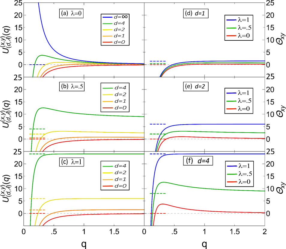
Figure 1: Variation of potential $U^{(x,y)}_{(d,\lambda)}(q)$ with $q$ for different values of $d$ and $\lambda$. Heights of the dashed short horizontal lines in each figure indicate the lowest eigenvalues for $\Theta_{xy}$ for the corresponding (color matched) potential.

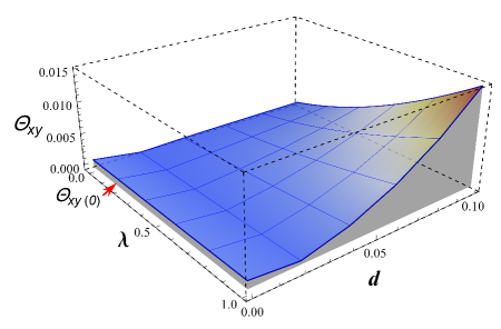
Figure 2: $\Theta-d-\lambda$ diagram shows a non-zero minimum value $\Theta_{xy(0)}\approx 0.002$ .

Heisenberg Uncertainty Relation for anyon: The details of the computation of $\Delta r^{2}$ are provided in Supplemental Material. As before, we exploit the spherical symmetry by introducing polar coordinates,

$$N^{2}=\int^{\infty}_{0}dp~{}p\int^{2\pi}_{0}d\theta~{}\mid v(p,\theta)\mid^{2}d\theta$$ (29)

$$\Delta p^{2}=\frac{1}{N^{2}}\int^{\infty}_{0}dp~{}p\int^{2\pi}_{0}d\theta~{}p^{2}\mid v(p,\theta)\mid^{2}$$ (30)

$$\Delta r^{2} =\frac{1}{N^{2}}\int^{\infty}_{0}dp~{}p\int^{2\pi}_{0}d\theta$$ (31)

$$\left[p\mid\partial_{p}v(p,\theta)\mid^{2}+\frac{1}{p}\mid\partial_{\theta}v(p,\theta)\mid^{2}\right.$$

$$+\left(-\frac{p^{3}}{E^{4}}+\lambda~{}p\left(\frac{1}{E^{2}}+\frac{2\lambda+1}{m^{2}}\right)\right.$$

$$\left.-\frac{4(\lambda-1)(E-m)(E\lambda+m)}{mEp}\right)\mid v(p,\theta)\mid^{2}$$

$$-i\frac{m(\lambda-1)(m-E)+\lambda p^{2}}{mEp}v^{*}(p,\theta)\overleftrightarrow{\partial_{\theta}}v(p,\theta)].$$

Following bel we define $\bar{\Theta}_{xp}=\sqrt{\Delta r^{2}\Delta p^{2}}/\hbar$ and try to find the minimum value of $\bar{\Theta}_{xp}$ by varying $v^{*}$ and equating it to zero. For the same reasons mentioned earlier we invoke spherical symmetry since angular contributions can only increase the eigen value bel . The variational equation for $\Delta r^{2}\Delta p^{2}$ with respect to $v^{*}$ reduces to

$$\left[\Delta p^{2}\left(-\partial^{2}_{p}-\frac{1}{p}\partial_{p}-\frac{p^{2}}{E^{4}}-\frac{4(\lambda-1)(E-m)(E\lambda+m)}{Emp^{2}}\right.\right.$$

$$\left.\left.+\lambda\left(\frac{1}{E^{2}}+\frac{2\lambda+1}{m^{2}}\right)\right)+p^{2}\Delta r^{2}-2\bar{\Theta}_{xp}^{2}\right]v(p)=0.$$ (32)

Shifting to dimensionless variables bel $q=\frac{p}{mcd},~{}d=\frac{1}{mc}\left(\frac{\hbar^{2}\Delta p^{2}}{\Delta r^{2}}\right)^{1/4}$ we recover a Schrodinger-like equation for $v_{(d,\lambda)}(q)$

$$\frac{1}{2}\left[-\partial_{q}^{2}-\frac{1}{q}\partial_{q}+2U^{(r,p)}_{d,\lambda}(q)\right]v_{(d,\lambda)}(q)=\bar{\Theta}_{xp}v_{(d,\lambda)}(q)~{}~{}~{}~{}~{}$$ (33)

where the potential is

$$2U^{(r,p)}_{(d,\lambda)}(q)=-\frac{q^{2}d^{4}}{(1+q^{2}d^{2})^{2}}+\lambda d^{2}\left(\frac{1}{q^{2}d^{2}+1}+2\lambda+1\right)$$

$$-\frac{4(\lambda-1)(\sqrt{q^{2}d^{2}+1}-1)(\lambda\sqrt{q^{2}d^{2}+1}+1)}{q^{2}\sqrt{q^{2}d^{2}+1}}+q^{2}$$ (34)

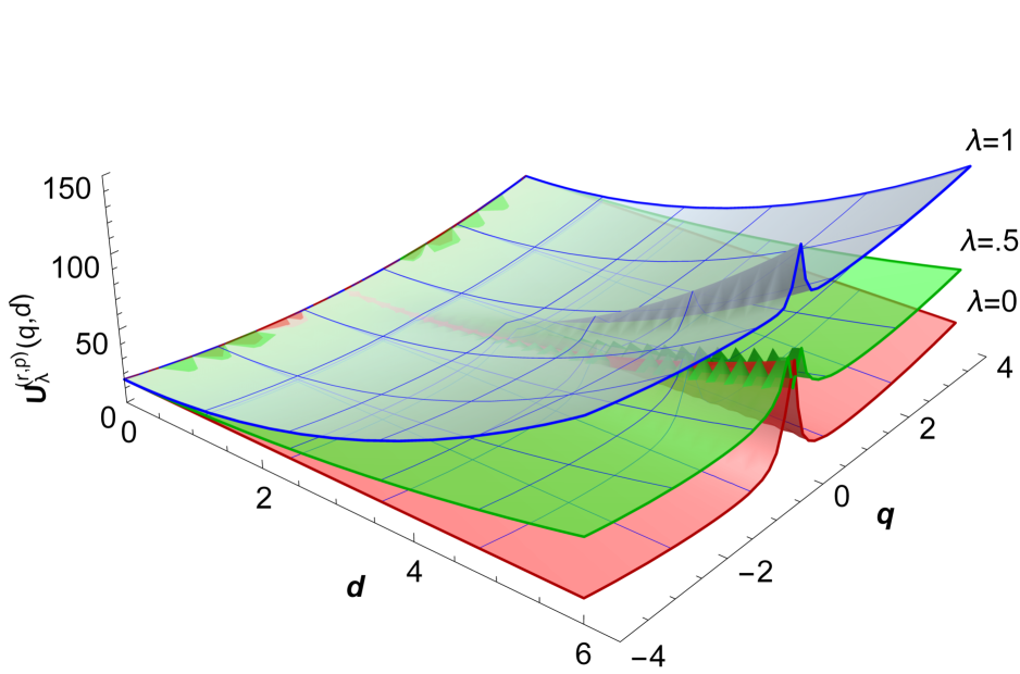
Figure 3: Variation of $U^{(r,p)}_{(d,\lambda)}(q)$ with $q$ and $d$ for different values of $\lambda$ .

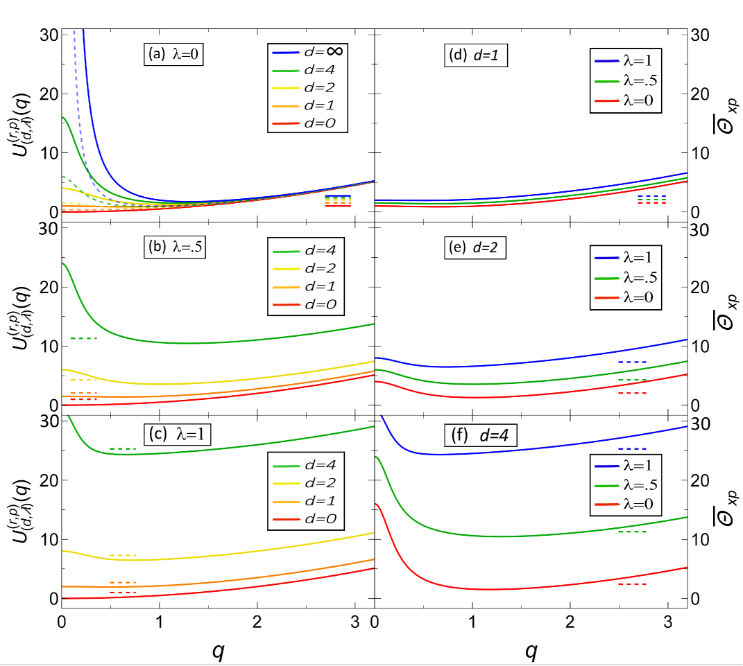
Figure 4: Potential $U^{(r,p)}_{(d,\lambda)}$ vs. $q$ is plotted for different values of $d$ and $\lambda$. Heights of the dashed short horizontal lines in each figure indicate the lowest eigenvalues for $\bar{\Theta}_{xp}$ for the corresponding (color matched) potential. In Fig. (a), the eigenvalues for the limiting cases $d=0$ and $d=\infty$ for $\lambda=0$ are denoted by solid lines. Dotted curves in (a) represent the potential term for electron, as given in Ref.bel , for the same values of $d$.

Notice that $d\rightarrow 0$ yields the non-relativistic limit, for which (33) becomes independent of $\lambda$,

$$\frac{1}{2}\left[-\partial_{q}^{2}-\frac{1}{q}\partial_{q}+q^{2}\right]v_{0}(q)=\bar{\Theta}_{xp(0)}v_{0}(q)$$ (35)

Incidentally (35) is identical to the corresponding equation for electron in bel apart from a factor of $2$ in the $\partial_{q}/q$ term for space dimensional mismatch. The solution of the above equation is a Gaussian $v_{0}(q)=exp(-q^{2}/2)$ with the lowest eigenvalue $\bar{\Theta}_{xp(0)}=1$. We recover the HUR for anyon as $\sqrt{\Delta r^{2}\Delta p^{2}}=\hbar$, due to the two (spatial) dimensional nature of the system. This is one of our major results.

It is interesting to note that the relativistic limit $d\rightarrow\infty$ exists only for $\lambda=0$ (i.e. for spin $s=1-\lambda=1$, otherwise some $\lambda$-dependent terms diverge) leading to

$$\frac{1}{2}\left[-\partial_{q}^{2}-\frac{1}{q}\partial_{q}+q^{2}+\frac{3}{q^{2}}\right]v_{(\infty,0)}(q)=\bar{\Theta}_{xp(\infty,0)}v_{(\infty,0)}(q)$$

(36)

The solution of the above differential equation is $v_{(\infty,0)}(q)=q^{\sqrt{3}}e^{-q^{2}/2}$ and $\bar{\Theta}_{xp(\infty,0)}=1+\sqrt{3}$. A few representative results are given in tabular form

	$\lambda=0$	$\lambda=0.5$	$\lambda=1.0$
d=0	1.0	1.0	1.0
d=1	1.54	2.08	2.69
d=2	2.05	4.29	7.29
d=4	2.41	11.29	25.31
d=$\infty$	2.73	-	-

Table 1: Lowest eigen values for different values of $d$ and $\lambda$

In Fig.(3) a three dimensional plot for $U^{(rp)}_{(d,\lambda)}(q)-q-d$ for different $\lambda$ shows how the potential separates in to sheets for each $\lambda$. In Fig.(4) variations of $U^{(rp)}_{(d,\lambda)}$ with $d$ and $\lambda$ are shown along with corresponding eigenvalues $\bar{\Theta}_{xp}$. The anyon results are new and can be compared with similar results for electron bel . These constitute our second major result for anyon.

Anyon equation of state and the NC parameter $\Theta_{xy}$ : Using the relations derived above let us consider

$$\frac{\Theta_{xy}}{\Delta x^{2}}=\frac{\Theta_{xy}\hbar^{2}}{\Delta p^{2}}\approx\frac{\Theta_{xy}\hbar^{2}}{mkT}.$$ (37)

One might identify the above with the thermal de Broglie wavelength $\lambda={\sqrt{(2\pi\hbar^{2})/(mkT)}}$. This can play a part in the discussion below.

In statistical mechanics, ideal gases where particles are treated as non-interacting, play an important role. In the quantum version, the Fermi/Bose statics effect is taken in to account in the otherwise non-interacting Fermi/Bose gas. These analysis require the multiparticle wave functions that are simply products of single particle wave functions for Fermions/Bosons. However, following the same procedure for anyons is not possible because single anyon wave functions do not yield the multi-anyon wave function in any simple way. Thus, one considers an ideal anyon gas as an interacting Bose/Fermi gas. The generic equation of state of an ideal gas in two space dimensions, is $(PA)/(NkT)=ln{\cal{Z}}$. $P,A$ are the pressure and area respectively, $N$ the particle number and $T$ the temperature. ${\cal{Z}}$ is the grand partition function. However, for anyons, considering an interacting system of Boson/Fermion the equation of motion is expressed as a series

$$\frac{P}{\nu kT}=1+a_{2}(\nu\lambda^{2})+a_{3}(\nu\lambda^{2})^{2}+~{}....$$ (38)

where $\nu=N/A$ is the number density, $\lambda$ the thermal wavelength and $a_{i}$ the (dimensionless) virial coefficients, leading to

$$\frac{P}{\nu kT}=1+a_{2}(\nu\Theta_{xy})+a_{3}(\nu\Theta_{xy})^{2}+~{}....~{}.$$ (39)

(For a detailed discussion see khare .) The above is a heuristic presentation of a possible significance of $\Theta_{xy}$, the anyonic spatial uncertainty parameter.

Commutative space for electrons: Let us check the consistency of our scheme by recovering the commutative space for electrons, in the framework of bel . Using free spinor solutions $F_{\alpha}^{+}$ for electron, the dispersion for $x$ and $y$ are straightforward to obtain. The expression simplifies considerably by invoking spherical symmetry $(f(p,\theta,\phi)=f(p))$,

$$\Delta x^{2}=\Delta y^{2} =\frac{4\pi}{3N^{2}}\int_{0}^{\infty}dp~{}\sum_{s}\left[p^{2}\mid\partial_{p}f(p)\mid^{2}\right.$$ (40)

$$\left.+\left(1+\frac{m}{E}+\frac{m^{2}p^{2}}{4E^{4}}\right)\mid f(p)\mid^{2}\right]$$

Let us define

$$\Delta x^{2}\Delta y^{2}=\hbar^{2}\bar{\Theta}_{xy(e)}^{2}$$ (41)

where $\bar{\Theta}_{xy(e)}$ is the NC parameter of dimension $(length)^{2}$ (if it turns out to be non-zero) and $e$ stands for electron. Integrating over $\theta$ and $\phi$ and considering the variation with respect to $f^{*}$ we have

$$\left[\Delta x^{2}\left(-\partial_{p}^{2}-\frac{2}{p}\partial_{p}+\left(\frac{1}{p^{2}}-\frac{m}{Ep^{2}}\right.\right.\right. \left.\left.\left.+\frac{m^{2}}{4E^{4}}\right)\right)\right]f(p)$$ (42)

$$=\Theta_{xy(e)}^{2}f(p)$$

where, $\Theta_{xy(e)}=\frac{\bar{\Theta}_{xy(e)}}{2}$ Introducing the dimensionless variable $q=\frac{p}{mcd}$ and parameter $d=\frac{1}{mc}\left(\frac{\hbar^{2}\Delta x^{2}}{\Delta y^{2}}\right)^{1/4}$, the above equation reduces to

$$\left[-\partial_{q}^{2}-\frac{2}{q}\partial_{q}+V^{(x,y)}_{d}(q)\right]f_{d}(q)=\Theta_{xy(e)}f_{d}(q)~{}~{}~{}$$ (43)

$$V^{(x,y)}_{d}(q)=\frac{1}{q^{2}}-\frac{1}{q^{2}\sqrt{1+d^{2}q^{2}}}+\frac{d^{2}}{4(1+q^{2}d^{2})^{2}}~{}~{}$$ (44)

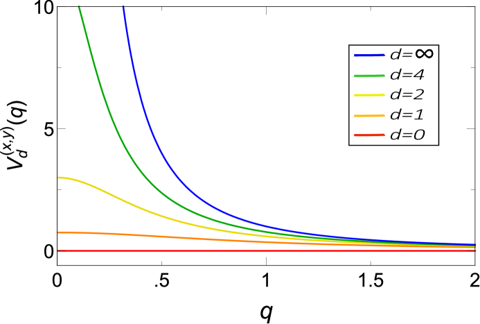
Figure 5: Variation of the potential $V^{(x,y)}_{d}(q)$ with $q$ for different values of $d$.

In Fig.(5), the profile of $q~{}vs.~{}V^{(x,y)}_{d}(q)$ for different values of $d$ is shown. For $\infty\geq d\geq 0$, the potential approaches zero for large $q$.

In the two limits of $d$, Eq.(43) reduces to

$$\left[-\partial_{q}^{2}-\frac{2}{q}\partial_{q}\right]f_{0}(q)=\Theta_{xy(e,0)}f_{0}(q),~{}~{}d\rightarrow 0~{}~{}~{}~{}~{}~{}~{}~{}~{}~{}~{}~{}~{}~{}~{}~{}$$ (45)

$$\left[-\partial_{q}^{2}-\frac{2}{q}\partial_{q}+\frac{1}{q^{2}}\right]f_{\infty}(q)=\Theta_{(e,\infty)}f_{\infty}(q),~{}d\rightarrow\infty.$$ (46)

We are interested in the smallest eigenvalue and clearly $\Theta_{xy(e,0)}<\Theta_{xy(e,\infty)}$ (due to the positive contribution from $1/q^{2}$ in (46) and the lowest possible value for $\sigma_{0}$ is zero consistent with free particle solution $f_{0}\sim exp[-i\sqrt{\Theta_{xy(e,0)}}q]$ for large $q$. Comparison with electron $\Delta r^{2}\Delta p^{2}$ HUR results in bel reveals that the presence of $q^{2}$ (harmonic oscillator) term in the overall potential that induced a non-zero minimum eigenvalue, is absent here in $\Delta x^{2}\Delta y^{2}$ HUR for electron. Thus $3+1-dim$ electrons live in a commutative space. Indeed, this is not a new result but rederived in the present framework, to be contrasted with the anyon result, derived earlier.

Conclusion and future prospects: To summarise, we have computed minimum values of products of dispersions between coordinates $x,y$ and between coordinate and momentum $r,p$ for $2+1$-dimensional arbitrary spin particles, referred to as anyons, utilising explicit form of anyon wavefunction jan , in the framework of bel . Non-zero value for the former yields the spatial uncertainty relation for anyon and strongly suggests that anyons live in noncommutative space. Incidentally we also show, in the same formalism, that Dirac electrons live in commutative space, which is reassuring. We have briefly indicated how $\Theta_{xy}$ might appear in anyon equation of state.

Indeed more research is required but still, it is tempting to interpret the noncommutativity parameter $\bar{\Theta}_{xy}$ as a new and independent constant for planar quantum physics, similar to $\hbar$ in phase space. It might be interesting to consider Zitterbewegung effect for anyons and also introduce Foldy-Wouthuysen or Newton-Wigner coordinates in the study of anyon.

More and more applications of anyons in modern physics, (especially in the area of quantum computing), makes it necessary to grasp the underpinnings of anyon theory at the microscopic level. We plan to extend our work to model an action principle for anyon that can be generalized to non-abelian anyons, the ultimate goal of this project.

Acknowledgements: It is indeed a pleasure to thank Professor Iwo Bialynicki-Birula for patiently explaining many subtleties of their work.
Data Availability Statement: No Data associated in the manuscript.

References

(1) R.Jackiw and V.P.Nair, Phys.Rev.D 43,1933(1991).
(2) M.S. Plyushchay, Phys.Lett.B 248,107(1990).
(3) J.Leinaas and J.Myrheim,
Nuovo Cimento Soc.Ital.Fis.37B,1(1977).
(4)F.Wilczek, Phys.Rev.Lett. 49,957(1982).
(5)Fractional Statistics and Anyon Superconductivity, F.Wilczek, Editor.
(6) J.Majhi, S.Ghosh and S.K.Maiti, Phys.Rev.Lett.123, 164801(2019).
(7) I.Bialynicki-Birula and Z.Bialynicka-Birula,
New J.Phys.21,07306(2019).
(8)I.Bialynicki-Birula and A.Prystupiuk,
Phys.Rev.A103,052211(2021).
(9) I.Bialynicki-Birula and Z.BialynickaBirula,
Phys.Rev.Lett.108,140401(2012).
(10) I.Bialynicki-Birula and Z.Bialynicka-Birula,
Phys.Rev.A 86,022118 (2012).
(11) M.Chaichian, R.G.Felipe, and D.L.Martinez,
Phys.Rev.Lett.71,3405 (1993);Erratum ibid.73,2009(1994).
(17) J.L.Cortes and M.S.Plyushchay, Int.J.Mod.Phys. A 11,3331(1996).
(18)R.Jackiw and V.P.Nair, Phys.Lett B551,166(2003).
(19) P.A.Horvathy and M.S.Plyushchay, Phys.Lett.B 595,547(2004).
(20)S.Deser, R.Jackiw and S.Templeton, Phys.Rev. Lett.48,975 (1982).
(21) A.J.Niemi and G.W.Semenoff, Phys.Rev.Lett. 51, 2077(1983).
(22) A.Stern, Anyons and the quantum Hall effect - a pedagogical review, cond-mat/0711.4697.
(23)E.J.ferrer, R.Hurka, V.de la Incera, Mod.Phys.Lett.B 11,1(1997).
(24)A.Yu.Kitaev, Ann. Phys.(N.Y.)303, 2 (2003).
(25)S. Rao, (2017) Introduction to abelian and non-abelian anyons; In S.Bhattacharjee, M.Bandyopadhyay (eds) Topology and Condensed Matter Physics. Texts and Readings in Physical Sciences, vol 19. Springer, Singapore.
(26) M.R.Douglas and N.A. Nekrasov, Rev.Mod.Phys.73,977 (2001).
(27) R.J.Szabo, Phys.Rep. 378,207(2003).
(28) R.Banerjee, B.Chakraborty, S.Ghosh, P.Mukherjee and S.Samanta, Found.Phys.39, 1297(2009).
(29) P.A.Horváthy, M.S. Plyushchay, M.Valenzuela, Ann.Phys. 325 (2010)1931.
(30) A.Khare, Fractional Statistics and Quantum Theory, 2005 World Scientific Publishing Co.
(31) Professor I.Bialynicki-Birula, private correspondence