StreamBlocks: A compiler for heterogeneous dataflow computing (Technical Report)

Abstract

To increase performance and efficiency, systems use FPGAs as reconfigurable accelerators. A key challenge in designing these systems is partitioning computation between processors and an FPGA. An appropriate division of labor may be difficult to predict in advance and require experiments and measurements. When an investigation requires rewriting part of the system in a new language or with a new programming model, its high cost can retard the study of different configurations. A single-language system with an appropriate programming model and compiler that targets both platforms simplifies this exploration to a simple recompile with new compiler directives.

This work introduces StreamBlocks, an open-source compiler and runtime that uses the Cal dataflow programming language to partition computations across heterogeneous (CPU/accelerator) platforms. Because of the dataflow model’s semantics and the Cal language, StreamBlocks can exploit both thread parallelism in multi-core CPUs and the inherent parallelism of FPGAs. StreamBlocks supports exploring the design space with a profile-guided tool that helps identify the best hardware-software partitions.

I Introduction

The slowdown in performance gain of general-purpose processors has increased interest in using FPGAs as reconfigurable accelerators, particularly for cloud computing [1, 2, 3, 4, 5].

A key challenge in designing these accelerators is partitioning computation between processors and an FPGA. An appropriate division of labor may be difficult to predict and only be revealed by experiments and measurements. When such an experiment requires rewriting part of a system in a new language, or with a new programming model, to run on the other platform, the high cost of exploration may retard studies of different configurations and limit the evaluation. A possible solution is a single-language system with an appropriately portable programming model and a compiler to generate code for both platforms. In this case, exploring a new system configuration just entails recompiling with new compiler directives.

A fundamental aspect is the programming model, which must allow parts of a program to run on either a CPU or an FPGA and interact transparently, regardless of where they execute.

The widely used accelerator model fails in two aspects. The different programming models for the CPU and FPGA make retargeting and design-space exploration costly and asymmetric. It requires rewriting a function in a new language or dialect to reimplement it for hardware. Also, it only supports a limited control transfer and communication model in which the CPU passes tasks to the accelerator. A component running on an FPGA cannot use the CPU as a coprocessor. However, industry flagship tools such as Xilinx SDAccel/Vitis and Intel OpenCL for FPGAs support this model for FPGA accelerators and MPSoCs.

Hardware could support more general models, such as concurrently processing multiple requests with pipelining or even out-of-order execution. However, these models integrate poorly with sequential programming languages such as C/C++ that natively support only sequential function calls.

One approach adopted by High-Level Synthesis (HLS) tools [6, 7, 8] to support other models is to introduce streaming or dataflow programming through a library. The hardware synthesized from C functions (C-HLS) runs concurrently with the software components and communicates through FIFO channels. The sequential semantics of C/C++, however, imposes limitations on the streaming functions [9]: (i) streams can only be single-producer, single-consumer [10], (ii) streaming functions cannot be bypassed, (iii) no backward links (feedback) between functions, and (iv) conditional reading of a stream may prevent concurrent execution. In other words, some patterns of execution that are natural for hardware are not expressible in a C function.

A workaround is to independently synthesize multiple streaming C-HLS functions with an HLS tool and manually connect the generated RTL modules with queues. Each design requires a custom script to produce its streaming network, and this script must evolve in step with the design. Moreover, because the network of streaming functions may not have an explicit enter (call) or exit (return) point, unlike a C-HLS function, code must be rewritten to handle end-of-stream marks.

This work introduces an alternative approach based on StreamBlocks, a compiler suite for heterogeneous dataflow programs. It enables the seamless hardware or software execution of streaming functions written in a single source language.

StreamBlocks starts with a dynamic dataflow programming language (Cal [11]). A dataflow program is a directed graph (cyclic or acyclic) whose nodes are operators called actors and edges are streams. A dataflow program specifies a partial order of computation, in which sequencing constraints arise only from data dependencies. As a result, actors can execute concurrently.

A dataflow program can be compiled to run on a processor, FPGA, or a combination of the two. In addition, dataflow semantics do not constrain an FPGA to operate only as a simple call-respond accelerator. It allows the FPGA to operate as a streaming coprocessor that executes concurrently with the processor and possibly invokes operations implemented in software. This generality allows the direct migration of part of a computation from software to hardware without rewriting the (dataflow) program, a essential step in developing, evaluating, or evolving a heterogeneous system.

However, the design space of possible partitions of functionality between the two platforms can be large and complex. StreamBlocks includes a profile-guided tool to help identify the best-performing ones.

The contributions of this work are:

• An open-source dataflow compiler for the Cal programming language that targets heterogeneous platforms.

• An automatic partitioning methodology for placing computations on heterogeneous platforms without rewriting code.

• A tool that uses this flexibility to find high-performing hardware-software partitions of a system.

• Experimental results demonstrating that our compiler can efficiently use the resources of a heterogeneous platform.

The paper is organized as follows. Section II provides an overview of dataflow programming and the actor machine. Section III presents the StreamBlocks compiler, heterogeneous code generation, and partitioning. Section IV compares StreamBlocks with other systems. Section V evaluates the compiler and partitioning. The paper concludes with Section VI.

II Dataflow, actors, and actor machines

Dataflow is a computation model used to express concurrent algorithms operating on streams of data. It has a rich history with many variants (e.g., [12, 13, 14, 15]) often targeted at a specific application domain or designed to facilitate efficient analysis or implementation. In our work, we use a general form of dataflow, in which a program is a network of computational kernels, called actors, that are connected via input and output ports by directed, point-to-point connections or channels (e.g., Fig. 1). Actors may have an internal state that is invisible to other actors. They interact exclusively by sending packets of data called tokens along the channels. Channels are lossless and preserve the order in which tokens are sent. They are also buffered (conceptually with unbounded capacity) so that the producer and consumer of a token need not synchronize during a transfer. A token may be consumed any time after it is produced.

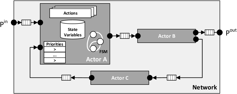
Figure 1: Structure of a Cal dataflow program.

Similar to the model introduced by Jack Dennis [12], the actors considered in this paper execute in a sequence of atomic steps or firings. During each step, an actor may (a) consume input token(s), (b) produce output token(s), and (c) modify its internal state. Instead of being written as a sequential process (e.g., Kahn processes [13]), languages such as Cal are structured around the steps an actor may perform. In Cal, an actor is a collection of actions, each describing a step that the actor can perform, along with the conditions under which the step should execute.

II-A Cal Actor Language

The Cal actor language [11] is a programming language for expressing actors with firing, the subject of this paper. It permits the description of actors for a wide range of dataflow models, ranging from Kahn process networks [13], dataflow process networks [14], and synchronous and cyclo-static dataflow [17, 15, 18], among others. Parts of the language have been standardized by the ISO/IEC committees RVC-CAL [19] as one of the languages used to write the reference implementations of MPEG video decoders.

⬇

namespace example:

external function rand(int x) --> int end

actor Source() int IN ==> int OUT:

int x := 0;

action ==> OUT:[rand(x)]

guard

x < 4096

do

x := x + 1;

end

end

actor Filter(int param) int IN ==> int OUT:

function pred(int param, int value) --> bool :

if (param > value) then true else false end

end

t0: action IN:[t] ==> OUT:[t] guard pred(param, t) end

t1: action IN:[t] ==> end

priority

t0 > t1;

end

end

actor Sink() int IN ==> :

action IN:[x] ==> do println(x) end

end

network TopFilter(int param) ==>:

entities

source = Source();

filter = Filter(param=param);

sink = Sink();

structure

source.OUT --> filter.IN;

filter.OUT --> sink.OUT;

end

end

Listing 1: A simple network of two actors in Cal.

Listing 1 contains a Cal dataflow program composed of four entities: three actors and a network. Actor Source has a single output port OUT. Its single action describes the only step it takes, incrementing a state variable x up to 4096 and producing a token to be sent to its output port. The token contains value from invoking the external function (rand) on x. External functions provide access to libraries and legacy code in a dataflow program.

The Filter actor’s parameter, param, is a number used by the local function pred. Filter uses an input port IN and an output port OUT. It comprises two actions. The first, labeled t0, includes a guard condition, a logical expression that must be true (in addition to an input token being available) for the actor to be able to take the action—copying the input token to the output. The second action, labeled t1, also consumes an input token but has no guard and produces no output. A priority rule specifies that action t0 has a higher priority than action t1. This means that whenever conditions for both are satisfied, action t0 executes. In this way, action t0 copies to the output all input tokens that satisfy its guard, while action t1 “swallows” the other tokens. Finally, Actor Sink consumes a token from its input port IN and prints it to the console.

The TopFilter network connects the three actor instances. The dataflow network in TopFilter has no input and output ports. It has three entities source, filter, and sink, which are instantiations of actors Source, Filter, and Sink, respectively. The filter instance is instantiated with a parameter received from the network.

The TopFilter network connects the IN input port of the network to the input IN of the rand instance. The output port OUT of instance source is connected to the input port IN of filter instance. The filter output port OUT is connected to the input port IN of the instance sink. This paper will use this Cal example to explain our work.

II-B Actor Machines

Executing an actor such as Filter alternates between two phases: (1) selecting the next action to execute and (2) executing it. In general, the choice of the next action can depend on many conditions (i.e., availability of input tokens, satisfiability of action guards, and availability of space in the output buffers) and might be ordered by priorities. At each point in time, zero, one, or more actions can be executed. If zero, action selection waits for an external event (arrival of input or freeing of output buffer space) to make an action executable. If more than one action can be executed, any can be chosen.

The actor machine (AM) [20] is an abstract machine model for actors that codifies the action selection process in a state machine called its controller. While an action’s execution is a single atomic step of an actor, it usually requires several microsteps of an AM to evaluate and test (and possibly re-evaluate and re-test) conditions until it can finally select and execute an action.

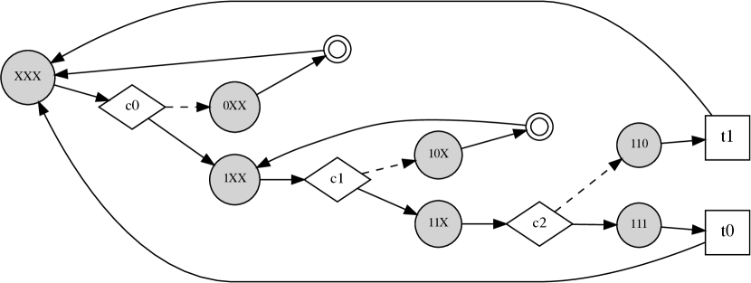
Figure 2: Controller state machine for the Filter actor in Listing 1. The gray circle, diamond, square, and ring respectively represent state, TEST, EXEC, and WAIT.

Fig. 2 shows a controller for the Filter actor from Listing 1. Its execution depends on three conditions: $c_{0}$, the availability of a token on the input port, $c_{1}$, the availability of space on the output port, and $c_{2}$, the guard of the first action. In the figure, the shaded circles represent the controller states, while the diamonds, boxes, and rings represent the three kinds of controller instructions that transition the controller from one state to another:

1. TEST: tests a condition (either presence of input, availability of output space, or a guard condition) and takes the controller to one of two states depending on whether the condition is true or false,

2. EXEC: executes an action and transitions to a new controller state,

3. WAIT: transitions to a new controller state.

Only an EXEC microstep changes the program-defined state of an actor machine (i.e., the internal state variable assignments and the streams connected to its ports).

Every state of an AM controller corresponds to a specific configuration of knowledge about the conditions, each of which may be true, false, or unknown (represented by $1$, $0$, and $X$, respectively). In the example, each controller state is labeled with a triple of values from $\{0,1,X\}$, corresponding to what is known about $c_{0}$, $c_{1}$, and $c_{2}$ at that point in the controller’s execution. For example, the initial controller state, when nothing is known, is labeled $XXX$. Once the first condition, $c_{0}$ is tested and it is known whether there is an input token, the controller transitions to either $0XX$ (no input token) or $1XX$ (input token available). If in the process of checking conditions, the controller ends up in a state in which it can perform an EXEC instruction, it has successfully selected an action. The EXEC instruction then executes the action, and the selection process begins anew.

If the controller ends up in a state such as $0XX$, nothing can be done until an input token arrives. When something outside of the AM changes, the AM condition needs to be re-tested. This means the AM controller needs to “forget” that there was no input token and return to the initial state $XXX$ to re-test. This is the role of the WAIT instruction, which “throws away” knowledge about transient conditions (i.e., conditions that can change through things happening outside of the AM, such as tokens arriving or output space becoming available), so they can be re-assessed. A WAIT instruction is typically used when the controller comes to a point at which it cannot execute an action or test additional conditions that would enable it to perform an action. In other words, the controller is stuck until some external occurrence changes one of its transient conditions.

The AM in Fig. 2 contains exactly one instruction in each state (a so-called single instruction AM, or SIAM). In general, AMs that allow a choice of multiple instructions to proceed from a controller state (multiple instruction Actor Machine, or MIAM) makes the controller non-deterministic. In this paper, the actor machines of a CAL actor use only a single instruction (SIAM) for each state to reduce the number of tests needed at runtime. A detailed discussion of the relationship between single instruction and multiple instruction machines can be found elsewhere [21]. All that matters for this paper is that any MIAM can be reduced to a SIAM that maintains the actor’s original semantics while possibly reducing the behaviors it may exhibit.

II-C AM Network and Idleness

AMs can be connected to create a network of AMs. The TopFilter actor in Listing 1 is an AM network expressed in CAL, with two actors rand and filter. As apparent in Listing 1, so long as the Filter actor has input, it continues to take actions. In fact, this actor never terminates but simply waits when its input stream is empty. It resumes taking actions when additional tokens are fed into its input. If an actor stops working due to an absence of external events, we say the actor became idle.

With a single AM, the controller state machine can check for idleness. An AM is idle if its controller state machine can only perform sequence of TEST steps ending with a WAIT in absence of external events. However, reasoning about idleness in a network of AMs is more subtle, especially in presence of cycles in the network and unpredictable token production/consumption, a characteristic of AMs.

Idleness is an important property because if a hardware AM network can autonomously detect its idleness, then software need not continuously poll to see if hardware has completed an operation. Since, in general, a hardware network can produce a (statically) unknown number of output tokens, without a method to detect when the hardware is finished (idle), software must continually poll for results or end-of-streams be explicitly baked into the code by programmers. The StreamBlocks compiler implements a run-time mechanism to efficiently detect idleness on hardware without software intervention.

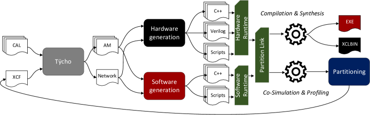
Figure 3: StreamBlocks heterogeneous compilation flow. The compilation and synthesis results in a multi-threaded executable that asynchronously launches an OpenCL RTL kernel (XCLBIN). The XCF configuration file can either be specified by a user or generated automatically by the partitioning tool..

III StreamBlocks

StreamBlocks is a suite of tools for designing, compiling, and optimizing streaming dataflow applications. The framework consists of three parts: Cal compiler front-end, back-end code generators, and a partitioning tool. The Cal front-end comes from Tÿcho [16] and supports a common representation based on the AM machine model on which to perform transformations and optimizations. Both imperative and action-based kernels can be translated to this representation, making the same optimizations applicable to different types of kernels and across language boundaries. StreamBlocks extended Tÿcho with a type system that supports Product and Sum types similar to those in functional programming languages.

Tÿcho produces an AM representation, which is fed to the homogeneous/heterogeneous StreamBlocks back-ends to apply platform-specific transformations (Section III-B and III-C). Each platform supports a runtime responsible for actor scheduling. Hardware actors are scheduled in parallel whereas software actors are scheduled on cores following a user-provided, actor-to-core mapping. An XML configuration file specifies these actor-to-core or actor-to-FPGA mappings.

The final aspect of StreamBlocks is partitioning (Section III-F). Each runtime supplies methods for profiling a dataflow application on its platform (Section III-E). Profiling uses either hardware cycle timers for CPUs or cycle counts from a cycle-accurate RTL simulation. Also, StreamBlocks provides tools for profiling inter-actor communication on a heterogeneous platform. The StreamBlocks partitioning uses profiling information to map actor instances to the processing cores in a homogeneous platform or across processing cores and FPGA on a heterogeneous platform.

Finally, this paper focuses on software and hardware code generation for heterogeneous platforms that support the Xilinx OpenCL runtime, i.e., any Xilinx PCIe accelerator board or MPSoC.

Listing 2: Configuration file for the TopFilter network.

⬇

<?xml version="1.0" encoding="UTF-8" standalone="yes"?>

<configuration>

<network id="example.TopFilter"/>

<partitioning>

<partition id="0" pe="x86_64"

code-generator="sw">

<instance id="sink"/>

</partition>

<partition id="1" pe="xczu7ev-ffvc1156-2-e"

code-generator="hw">

<instance id="source"/>

<instance id="filter"/>

</partition>

</partitioning>

<code-generators>

<code-generator id="sw" platform="multicore"/>

<code-generator id="hw" platform="vivado-hls"/>

</code-generators>

<connections>

<fifo-connection source="source" source-port="OUT"

target="filter" target-port="IN"

size="1"/>

<fifo-connection source="filter" source-port="OUT"

target="sink" target-port="IN"

size="4096"/>

</connections>

</configuration>

III-A Configuration File

A developer can use source-code annotations to force the placement of Cal actors on either hardware or software. It is also possible to partition actors between hardware and software using a StreamBlocks XML Configuration File (XCF). For example, Listing 2 shows a mapping of the TopFilter network from Listing 1. Source and Filter execute on the FPGA and Sink on the CPU. Most actors can run on either platform, but some cannot be placed on hardware, for example, an actor that reads a file.

The configuration file specifies the Cal network partitioning, code generators, and connections. Each partition has an name (id), the id of the code generator to use, and the names of the Cal instances it contains. A code generator can be configured with platform-specific settings (i.e., desired clock frequency, maximum BRAM size, …). If these are not specified, the compiler uses a default value. There are two types of connections: FIFO connections and external memory connections. If the depth of a FIFO connection is not declared, the code generator is free to choose any value. External memory connections are used to hold large actor state variables, which do not fit in BRAM, in a memory bank on the FPGA PCIe accelerator board.

III-B Hardware Code Generation

The StreamBlocks compiler generates a C++ class for each Hardware AM (HAM). Listing 3 contains a class definition for actor Filter in Listing 1. The top function for HLS is operator(), which implements the AM controller state machine. The transition and condition functions implement the EXEC and TEST steps. The scope function sets variable assignments for actions and is invoked before the transition or condition functions.

We use Vivado HLS’s streaming library, hls::stream class, to implement the input and output ports for AMs. To execute an action, a controller state machine checks if (i) input tokens are available, (ii) there is space for the output, (iii) and guard conditions are satisfied. hls::stream does not offer appropriate functionality since its API does not allow reading the size of a stream or peeking at values without consuming them. To avoid these limitations, we created a custom Verilog First-Word Fall-Through (FWFT) FIFO whose outputs are its size, count, and head queue element and that is compatible with the hls::stream RTL input/output interface. To use these output values, a unique IO structure for each AM is generated and the count, size and queue are passed by value (io argument of the top HLS function) as shown in Listing 3.

The HLS implementation of a controller state machine follows its definition in Section II-B. At each invocation of operator(), the actor can take multiple steps or instructions. Its state is recorded in the variable program_counter to allow execution to continue between invocations.

Listing 3: C++ class and top HLS function for the Filter AM (Vivado/Vitis HLS).

⬇

struct IO{

int32_t IN_peek;

int32_t IN_count;

int32_t OUT_size;

int32_t OUT_count;

};

class class_filter {

private:

// -- State Variables

bool pred_1(int32_t l_param, int32_t l_value);

int32_t a_param, a_t__1, program_counter;

// -- Scopes

void scope_1(IO io);

// -- Conditions

bool condition_0(hls::stream< int32_t > &IN, IO io);

bool condition_1(hls::stream< int32_t > &OUT, IO io);

bool condition_2();

// -- Transitions

void transition_0(hls::stream< int32_t > &IN,

hls::stream< int32_t > &OUT);

void transition_1(hls::stream< int32_t > &IN);

public:

// -- For static instatiation

class_filter(int32_t param){ a_param = param; }

// -- Controller

int32_t operator()(hls::stream< int32_t > &IN,

hls::stream< int32_t > &OUT, IO io);

};

// -----------------------------------------------

// -- HLS Top Function, instantiated with param=10

int32_t filter(hls::stream< int32_t > &IN,

hls::stream< int32_t > &OUT,

IO io){

static class_filter i_filter(10);

return i_filter(IN, OUT, io);

}

Fig. 2 depicts the example’s controller state machine. This controller has two entry points, state $XXX$ and $1XX$, and 4 exit points, when the controller reaches the two wait states and after executing $t_{0}$ or $t_{1}$. Suppose that on invocation, the controller is in state XXX and all conditions $c_{0}$ to $c_{2}$ are true. Then, the controller performs TEST steps for $c_{0}$, $c_{1}$, and $c_{2}$, changing state accordingly to 1XX, 11X, 111. At state 111, it performs the EXEC step $t_{0}$, transitions to state XXX, returns a code that indicates its last step was an EXEC, and exits. The controller is acyclic; it does not execute the same step multiple times in a single invocation. Because the steps are bounded, the HLS scheduler (i.e., Vivado HLS) can schedule all TEST steps, $c_{0}$ to $c_{2}$, at the first clock cycle of invocation. To improve performance, the controller takes the maximum number of steps possible (without cycling) before it exits.

StreamBlocks automatically inserts some HLS directives (i.e., pragma) in appropriate places to optimize the hardware. For instance, all scope, condition, and transition methods are inlined in the controller. Also, loops with fewer than 64 iterations are unrolled to accelerate repeat expressions without incurring an unreasonable resource cost. A developer can also directly annotate the source code with other directives. For example, @loop_merge can be used to merge input-read and output-write loops, and @external can place an actor variable in an off-chip memory (e.g., DDR or HBM). In the latter case, the compiler produces appropriate HLS pragmas to add an AXI master interface to the actor.

FIFOs that cross the hardware/software boundary are connected to Input and Output Stage actors. These special actors transparently pass tokens between hardware and software without developer involvement (Section III-D).

Vivado HLS compiles each actor to RTL. The corresponding RTL actor is instantiated in a Verilog network along with its trigger module. The trigger is a hardware scheduler that enables or disables its actor. In hardware, ideally, all actors should execute asynchronously to maximize performance. However, hardware should also detect when forward progress is no longer possible (idleness) and inform software that computation is complete and output data is available.

We use the triggers to detect idleness. Detecting idleness in an actor network requires synchronized coordination. The triggers continually monitor network state and eventually perform a synchronized idleness check. Fig. 4 illustrates an example. ID, AT, and ST correspond to idle, asynchronous triggering, and synchronous triggering, respectively. In the normal state, AT, actors are repeatedly and asynchronously activated until all triggers in the network observe their actors are idle. When that happens, the triggers synchronously execute ST to check idleness and disable the network if it is the case. For conciseness, we omit details of our hardware idleness detection algorithm.

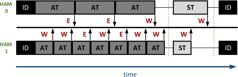
Figure 4: An example trace of the execution of two hypothetical HAMs. ID, AT, ST corresponds to idle, asynchronous trigger and synchronous triggering. E, W corresponds to EXEC, WAIT return codes from a HAM. Vertical green lines represent synchronization points.

In the Verilog network, actors communicate through FWFT queues. When the first token is written into a queue, it immediately appears on the output, thus it allows the token to be read on the next clock cycle. The FIFO’s data width is set automatically from the width of the outgoing and incoming ports of the connected actors. If the outgoing and incoming ports’ width differ, the compiler reports an error. The depth of all queues in the network is set to a compiler-defined value if the XCF configuration file does not specify it.

III-C Software Code Generation

Similar to hardware code generation, the StreamBlocks compiler translates a software AM (SAM) to a C++ class that runs on a processor. Our multi-threaded runtime instantiates each actor class. Conceptually, it seems appropriate to allocate a thread to each actor since they execute independently. However, the relatively high cost of context switches leads to sub-optimal performance since an actor’s controller may not run for long before it determines that the actor is still idle. A better use of resources is to map several actors onto a thread and run them sequentially such that the cost of a context switch can be amortized over a larger computation. However, if several of these actors could run concurrently, then the opportunity to improve performance by running in parallel is lost. The actor-to-thread mapping is specified in the XCF file. The threads are assigned to dedicated physical cores. Each pinned thread has an independent, round-robin scheduling loop for its actors. If no thread mapping is specified in the XCF, a single thread runs all actors.

Unlike hardware execution, in which the controller state machine cannot have cycles in a single invocation, to reduce scheduling overhead, the software controller state machine performs as many steps as possible. It may execute the same step multiple times, before yielding to the scheduler. The compiler has a default maximum threshold for iterating in the controller, which can be overridden by command-line arguments. In the case that an actor reaches a WAIT instruction before the threshold is hit, it yields earlier.

FIFOs are implemented as ring buffers. A structure attached to every AM output port holds global and local FIFO counters. The global counters are visible to all partition threads, but a local one is visible only to its thread. Global and local counters do not change while the actors are running. Updates are cached internally and synchronously applied after full iteration of the round-robin scheduling. This allows the FIFO ring buffers to be lock-less, as threads only see newly written/read-and-freed tokens after this step.

Fig. 5 shows the three steps of executing a thread in the software runtime. Pre-fire determines how much data can be read and written and stores the local FIFO counters’ values in its thread. Fire runs all SAMs in the partition in a round-robin scheduling iteration and makes visible all FIFO writes from the SAMs that fired during the iteration. Post-fire checks if a SAM executed in the Fire step, so other threads should wake up. If no SAMs executed in the Fire step, then the thread sleeps. If all other threads are asleep and all have had a “quiescent” round in which no tokens are produced or consumed, the threads terminate.

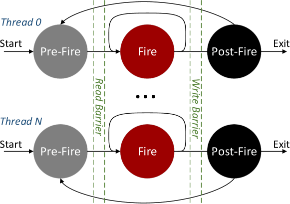
Figure 5: Pre-Fire, Fire, and Post-Fire steps for scheduling actors on a thread. Pre-Fire checks if a thread has sufficient data to execute. Fire runs the actors in the partition with a round-robin schedule, and Post-Fire checks if the thread should iterate, sleep or terminate.

The software runtime provides the threading mechanism and FIFO implementation. In addition, it supports system operations—such as file operations, image/video visualization, and other functionality—and links with library and legacy functions.

III-D Input/Output Stages and Partition Link

To enable actors to run on hardware or software, the compiler generates appropriate hardware/software interfaces. Fig. 6 depicts the interface architecture.

Figure 6: The hardware/software interface. Circles represent application actors. Arrows show communication paths. Input stage, output stage, and PLink are special actors that are instantiated depending on hardware/software actor placement.

PLink (Partition Link) is a special actor that (1) transfers software FIFOs to FPGA DDR memory, (2) starts the execution of hardware, and (3) receives data from the FPGA memory when the FPGA network becomes idle. A PLink treats the hardware network like a coprocessor and is its software controller. It invokes the coprocessor so long as the software continues to provide input values. Underneath, PLink takes advantage of OpenCL’s API [23], basically treating the hardware coprocessor as a kernel.

On the FPGA partition, for every incoming communication channel from software, we instantiate an input stage actor. These actors read data from the FPGA DDR memory in bursts which are then streamed to a BRAM FIFO connected to consumer actors. The output stage actor in Fig. 6 carries out a similar task and reads an FPGA FIFO corresponding to an outgoing communication paths and writes its values to DDR memory for the PLink to read. The input stage, output stage, and hardware actors constitute the dynamic region in Xilinx terminology. The dynamic region has multiple AXI memory ports with a single AXI slave port. The AXI slave port receives a start command from the PLink through OpenCL APIs (clEnqueueTask) and notifies it when the hardware execution becomes idle which is captured by the OpenCL runtime. The dynamic region is automatically wrapped by a static shell which connects all the AXI ports to appropriate blocks through the RTL kernel compilation flow of Vitis [24]. Bear in mind that the dynamic region changes by the hardware partition.

Additionally, when an FPGA actor requires DDR memory for object storage (e.g., an actor that uses a large array as an internal variable), the compiler instantiates appropriate memory interfaces. The PLink allocates the DDR memory on startup and passes the pointer to the hardware actor. Fig. 6 omits these details for clarity.

The PLink takes advantage of OpenCL events and an out-of-order command queue for nonblocking operations. All buffer transfers through clEnqueueWrite and clEnqueueRead and the starting of the kernel through clEnqueueTask have corresponding events. Consequently, the PLink never blocks the software thread it is scheduled on so that other actors can perform useful work.

III-E Testing & Profiling

The compiler provides a co-simulation solution that runs software actors on the software runtime and instantiates hardware actors as cycle-accurate SystemC models. A developer can test their heterogeneous application by simply specifying a compiler switch. We rely on Verilator to translate Verilog to SystemC. PLink transparently establishes the interface between the software and SystemC simulation domains. We do not yet model off-chip memory accesses, but will implement this feature in the future.

Co-simulation is also important for profiling hardware actors, which provides the basis for automatic hardware-software partitioning. The triggers in the SystemC network can optionally profile individual hardware actors. A trigger logs the minimum, maximum, and average clock cycles that an actor spends executing actions.

Likewise, the software runtime can profile similar information. The runtime uses the rdtscp time counter for x86 code, whereas ARM code uses the virtual cntvct counter scaled by clock frequency.

III-F Heterogeneous Partitioning

Finding an appropriate balance between hardware and software execution is a design space exploration problem part of hardware-software partitioning or hardware-software co-design. StreamBlocks facilitates this exploration process since an actor written in Cal can run in hardware or software with no code changes. In general, the design space is very large and raises several practical questions: (1) Which mapping of actors to software and FPGA produces the best performance? (2) Is it practical to find such partition(s) automatically?

Hardware/software partitioning can be modeled as a graph partitioning problem with a cost function. In this paper, we focus on execution time as the single metric to optimize, but a practical design must also balance resource usage, power, and other considerations. The cost function used in design space exploration should estimate the execution time for a given partitioning. Performance prediction is difficult for a variety of reasons: actors in Cal exhibit dynamic (sometimes even non-deterministic) behavior, the multi-threaded runtime can behave unpredictably, software-hardware crossings are difficult to model, and actors’ behavior is data-dependent because of dynamic data dependencies in and among actors.

To estimate multi-threaded software-hardware performance, we used a mixed integer linear programming (MILP) model. A model’s structure reflects the corresponding actor network graph. It is parameterized by profiling data (Section III-E) and measurements of software FIFO throughput and OpenCL host-to-device and device-to-host transfers.

We briefly present our model here, for more details refer to Section VII. Given a set of $n$ threads $P_{thread}=\{p_{1},p_{2},...,p_{n}\}$, an FPGA partition ${accel}$, and a set of actors $A$, we define the decision variables $d^{a}_{p}$ with the following constraints:

$$\forall a\in A,\forall p\in P_{thread}\cup\{{accel}\}:d^{a}_{p}\in\{0,1\}$$

$$\forall a\in A:\sum_{p\in P_{thread}\cup\{{accel}\}}d^{a}_{p}=1$$

The first constraint states that the decision variables are boolean and the second ensures that each actor $a$ maps to exactly one partition $p$.

The execution time of an actor $a$ on partition $p$ is given by $exec(a,p)$, which is obtained through software or hardware profiling. The time spent on a thread partition is the sum of all actor execution times since actors run sequentially on a thread:

$$\forall p\in P_{thread}:T_{p}=\sum_{a\in A}d^{a}_{p}\times exec(a,p)$$ (1)

We delegate the performance modeling of a hardware actor to the PLink actor described in Section III-D. We assume that all PLink operations are asynchronous and, without loss of generality, we assume PLink is always scheduled by $p_{1}$.

$$\begin{split}T_{plink}&=max(\{d^{a}_{accel}\times exec(a,accel)\})\\ &+T^{read}_{plink}+T^{write}_{plink}\end{split}$$ (2)

The first term models hardware execution time as the maximum of actor execution times since actors can run concurrently on the FPGA. The other two terms model OpenCL read and write transfers, which depend on the number of tokens and the OpenCL cost information. Note that although PLink’s operations are asynchronous, because there a logical dependence between write, execution and read, their total time is their sum.

Similar to the hardware performance, we model the multi-threaded execution time as the maximum of individual thread execution times:

$$\begin{split}T_{exec}&=max(\{T_{p}:p\in P_{thread}\}\cup\{T_{plink}\})\\ &+T_{intra}+T_{inter}\end{split}$$ (3)

Observe that $T_{plink}$ is not added to $T_{p1}$ since it operates asynchronously, however, if the hardware is slower than all software threads, then execution time is determined by hardware, hence the $max$ operation. The $max$ term models pure actor execution time with no regard for communication cost between actors. Actors that communicate heavily can exploit fast caches if they are assigned to the same thread. Actors on different threads will communicate through the shared (e.g., L3) cache or main memory. $T_{intra}$ and $T_{inter}$ model the latency of intra- and inter-core communication. The latter two terms help ensure that actors that communicate heavily reside on the same thread.

The terms $T_{intra}$ and $T_{inter}$ are MILP formulas that depend on the software FIFO bandwidth and the number of tokens that are transferred on each FIFO. Our software runtime provides this profiling information.

Using a MILP formulation enables us to incorporate other constraints into the search. For instance, we can constraint the solutions to have fewer than $m$ FIFOs crossing the hardware-software boundary. This might be important when an FPGA platform has a limited number of AXI master ports to off-chip memory.

IV Related work

Cal has been used in many studies that produce both software and hardware code. The earliest publication on hardware code generation is [25]. It used OpenDF and Forge HLS from Xilinx. Orcc [26] is another framework for RVC-CAL that focused on video streaming applications.

Another tool, Xronos [27], used an open-source version of Forge HLS to translate Cal to HDL, again using the Orcc compiler. Compared to OpenDF, Xronos completely supports the RVC-CAL language for hardware synthesis.

Exelixi [28] and the tool in [29] are also based on the Orcc compiler but use Vivado HLS instead of Forge as a target. Authors in [30] directly generated VHDL from the Orcc intermediate representation.

Listing 4: Action selection controller used in Orcc.

⬇

void Filter(int param, InputStream IN, OutputStream OUT){

if(IN.available_token(1) && pred(param, IN.peek_token(1))){

if(OUT.available_space(1))

t0();

} else {

if( IN.available_token(1) )

t1();

}

}

A key difference of this work from other dataflow-to-hardware efforts is our use of the AM model to select actions for execution. Other Cal tools use a “basic” controller model that checks each consecutive execution of an actor against all of its firing conditions to select the action to execute. Consider the actor Filter from Listing 1. Listing 4 shows how other Cal-to-hardware tools implement action selection. If an actor has many actions, the number of firing conditions increases, and the cost of action selection increases. As a consequence, the latency of the actor increases too. For example, consider when the Filter actor has an input token in its input port, but no space to write the output, and the pred function is true. The controller on Listing 4 will always check first if there is input and if the result of pred is true. If so, it fails because there is no output space and exits, thus, losing a cycle (or more depending on pred’s latency) by retesting these conditions when the controller is next started. By comparison, the AM controller remembers the conditions that were checked and so can execute action t1 when output space is available.

SysteMoC is an actor language [31] based on SystemC that facilitates classification of models of computation for hardware-software co-synthesis. SystemCoDesigner [32] is a fully automated hardware-software design space exploration framework for SysteMoC programs on single-core SoCs with an embedded FPGA. Our work targets a broader range of platforms, from heterogeneous, multi-core SoCs to datacenter FPGA-accelerated platforms.

TornadoVM [33] is a virtual machine for managing Java-based streaming tasks on heterogeneous platforms incorporating CPUs, GPUs, and FPGAs. It can dynamically reconfigure tasks written in Java on available hardware resources. It precompiles each task to an FPGA bistream and then dynamically reconfigures programs on different hardware based on run-time information and program input size. We perform a static partitioning in which multiple tasks can be offloaded to the FPGA, while their work only accelerates a single task at a time.

LINQits [34] takes a program written in LINQ and accelerates query operation with a template library of hardware accelerators for an embedded heterogeneous MPSoC. User-defined anonymous functions are plugged into the template libraries through HLS synthesis. Unlike our work, LINQits focuses on accelerating the whole program (or kernel) while StreamBlocks provides a flexible boundary for acceleration.

SCORE [35] pioneers time-domain multiplexing to fit applications that require more resources than what is available on FPGAs and uses loadtime and runtime techniques for scheduling and placement. However, SCORE does not envision multi-threaded heterogeneous execution.

Finally, TURNUS [36] is a design space exploration and optimization tool that uses a different methodology for partitioning a dataflow program. TURNUS uses post-mortem execution traces of a dataflow application and profiling information to find partitions for homogeneous platforms. StreamBlocks supports both homogeneous and heterogeneous partitioning.

V Evaluating Partitioning

			Throughput
Benchmark	Actors	FIFOs	hardware	single	many	unit	speedup	Domain
JPEG Blur	104	210	881.96	161.33	127.06	frames/second	5.47	Decoding/format conversion/stencil
RVC-MPEG4SP	60	123	1858.62	868.61	472.44	frames/second	2.14	Video Decoding
Smith-Waterman	8	30	12911.56	3967.07	204.39	alignments/second	3.25	Sequence alignment
SHA1	20	26	130.64	53.75	177.66	MiB/second	0.74	Encryption
Bitonic Sort	28	57	6443K	5215K	5477K	sort/second	1.23	Hardware sorting
FIR	34	45	56	7.2	0.16	MiB/second	7.8	1D convolution
IDCT	7	9	1612K	979K	2039K	macroblock/second	1.64	Inverse cosine transform

TABLE I: An overview of the benchmarks on Intel Xeon 6234 + Alveo U250.

We performed our experiments on two systems. The first was a single node in the ETH Zurich XACC cluster that contains an Intel Xeon Gold 6234 8-core (16-thread) 3.3GHz processor and an Alveo U250 accelerator card connected to the system through a Gen3 PCIe x16 slot. This system is representative of data center accelerator platforms, with a high-end processor and a large FPGA. To evaluate our approach for embedded systems, we used the ZCU106 development board containing an MPSoC with 4 ARM64 cores running at 1.2GHz and a medium-size FPGA.

V-A Benchmarks

We used a suite of benchmarks of varying complexity from different application domains. Table I summarizes these benchmarks, with performance on the U250 platform. The benchmarks differ widely:

• JPEG Blur performs 8 coarse tasks: parsing, Huffman decoding, dequantization, cosine transform, macro block to raster conversion, Gaussian blur filter, and raster to macro block conversion. The Gaussian blur kernel implementation is based on the work of Cong et al [37].

• RVC-MPEG4SP video decoder is a reference implementation of the RVC-MPEG4SP ISO/IEC 14496-2 MPEG-4 standard. This design has been used in many Cal-related publications. The decoder is composed of 7 sub-networks: parser, 3 texture decoding networks, and 3 motion compensation networks.

• Smith-Waterman is an implementation of the Smith-Waterman string matching algorithm for DNA alignment [38].

• SHA1 is a straightforward implementation of the SHA1 algorithm with eight SHA1 compute engines. Each engine has a padding actor and a compute actor.

• Bitonic sort is an eight-element bitonic sort implementation.

• FIR a 64-tap pipelined FIR filter.

• IDCT Inverse cosine discrete transformation used in video and image decoding.

The throughput numbers in Table I reflect three scenarios:

• hardware. All actors are placed on the FPGA with the exception of 2 or 3 actors that perform file and IO operations.

• single. All actors are placed on a single software thread.

• many. Each actor runs on its own thread, e.g., if there are 104 actors in a system, then 104 threads are spawned.

As evident in Table I, using a thread per actor frequently degrades performance because of the cost of thread scheduling and inter-thread communication. Furthermore, placing all actors in hardware does not necessarily result in the best performance. The three throughput measurements in Table I represent the three corners of the design space, but not necessarily the best performing points. In fact, we demonstrate that when multiple software threads work in tandem with the FPGA better performance is achieved.

Below, we focus only on JPEG Blur and RVC-MPEG4SP, as they are fairly large and contain a set of computational kernels with dynamic behavior.

V-B Design Space Exploration

In this section, we use the MILP formulation presented in Section III-F to automatically explore the design space of the JPEG Blur and RVC-MPEG4SP benchmarks on both platforms. To do so, we solve the MILP formulation for a fixed number of threads, with and without an FPGA. We vary the number of threads from 2-8 on the datacenter platform and 2-4 on the embedded platform the Xeon processor has 8 cores and the ARM processor has 4. This produces many multi-threaded software and multi-threaded heterogeneous partitions. To effectively utilize OpenCL read and write bandwidth, in the heterogeneous solutions we allocate 1-4 MiB OpenCL buffers. Inside the FPGA, FIFO sizes are set by the values in the Cal code or set to 4096 on Alveo U250 and 512 on ZCU106 (default value) if unspecified. Likewise, for multi-threaded software, we do not override the buffer configuration since buffers that do not span software and hardware are not as sensitive to payload size. The selection of buffer size is reflected in the in the MILP formulation. Without this design choice, hardware performance is severely bottlenecked by poor hardware-software data transfers and, in fact, the MILP optimizer fails to find meaningful hardware partitions.

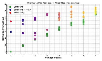
(a)

(b)

Figure 7: Evaluated JPEG Blur design points on (a) Alveo U250 and (b) ZCU106 platforms, each hardware partition has a unique color.

The MILP optimizer takes four inputs: (i) SystemC profile with per-actor clock cycle count obtained through co-simulation, (ii) software profile with per-actor timing information measured with CPU hardware counters, (iii) software FIFO bandwidth measured with CPU hardware counters, and (iv) OpenCL read and write bandwidth for a range of buffer sizes measured with OpenCL event counters. Observe that (i) is FPGA clock cycles, (ii) and (iii) are CPU cycles, and (iv) is nanoseconds. We convert all these numbers to nanoseconds by “guessing” a final FPGA operating frequency and using the advertised processor clock speed. The outcome of our experiments are summarized in Table II.

Benchmark			JPEG Blur	RVC-MPEG4SP
U250	baseline (fps)		161.33	868.61
	software	partitions	63	70
		speedup	6.90	4.78
	software + FPGA	partitions	67	66
		bitstreams	34	38
		speedup	7.68	4.40
ZCU106	baseline (fps)		22.13	109.87
	software	partitions	30	30
		speedup	3.83	3.92
	software + FPGA	partitions	17	14
		bitstreams	12	8
		speedup	27.14	14.44

TABLE II: Design space exploration summary of the JPEG Blur and RVC-MPEG4SP benchmarks on the U250 data-center and the ZCU106 embedded platforms. Speedup numbers correspond to the maximum performance achieved with and without hardware. Bitstreams counts the number of unique hardware partitions (which may have multiple software-thread partitions).

V-B1 JPEG Blur

Fig. 7 illustrates the various evaluated design points of the JPEGBlur benchmark on the Alveo U250 and ZCU106 platforms. On Alveo U250, there are 34 hardware partitions (i.e., one or more actors on hardware – bitstreams in Table II). Since the remaining software actors can be further partitioned across threads, there is a total of 67 heterogeneous partitions. Furthermore, we found 63 multi-threaded partitions that do not use hardware at all. On ZCU106, design space exploration yielded 30 software-only partitions and 12 hardware partitions resulting in 17 heterogeneous partitions.

The heterogeneous points in Fig. 7 are colored based on the hardware partition used at each point. The throughput is also normalized to the baselines reported in Table II.

Evidently, JPEG Blur can scale almost linearly with number of cores without hardware acceleration on both platforms. When an FPGA is used, scaling is not as well-behaved. We see a sub-linear speedup on Alveo U250 (Fig. 7a) where heterogeneous performance is better, in general. Conversely, heterogeneous performance slightly degrades with additional cores on the embedded ZCU106 platform (Fig. 7b). The best performance is the hardware-only design. Note that all of these alternatives were explored without code-rewriting or refactoring.

Fig. 7a demonstrates our claim that the optimum design point is not necessarily a hardware-only or software-only configuration, but rather a mixture. Without a common programming model to facilitate exploration of many partitions, exploring these design points would be a tedious process of code rewriting. Note, however, that due to the heuristic partitioning method, the discovered design points are not necessarily the global optimum either. Our claim is reinforced by Fig. 8, which depicts the best performing partition (on Alveo U250). This partition places a substantial number of actors on 6 software threads and boosts the speedup from about 5.5x (all hardware) to 7.7x. This non-trivial partition can be easily overlooked when partitioning takes place early in the implementation.

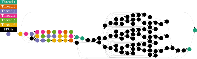
Figure 8: JPEG Blur configuration with the highest throughput.

V-B2 RVC-MPEG4SP

We discovered 66 heterogeneous partitions on Alveo U250, among which 38 correspond to a unique subset of actors on hardware. Without the FPGA, software partitioning yielded 70 configurations with 2-8 threads. With the ZCU106 platform, we found 30 software partitions and 14 heterogeneous partitions based on 8 unique hardware partitions. This experiment is summarized in Fig. 9, where the throughput is normalized to the single-thread execution in Table II.

RVC-MPEG4SP scales differently than the JPEG Blur benchmark on Alveo U250. Software enjoys linear acceleration up to 7 cores but then the performance drops, marking the limit of scalability. Similar to software scaling, the sub-linear heterogeneous scaling experiences a down-turn at 4 cores and eventually software performance surpasses heterogeneous performance.

On the ZCU106 platform, software scaling is almost perfectly linear for the 4 available cores. The heterogeneous performance sees a marginal increase with additional cores, unlike Fig. 7b, where heterogeneous performance experiences a slight dip with more cores.

We found a single-core heterogeneous partition that is 1.5x faster than an all-hardware solution, a point in the design space that could be easily overlooked.

The best heterogeneous Alveo U250 partition is outlined in Fig. 10. Such a valuable configuration may be simply left out in a manual development process.

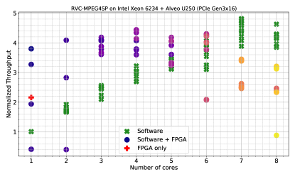
(a)

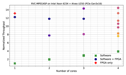
(b)

Figure 9: Evaluated RVC-MPEG4SP design points on (a) Alveo U250 and (b) ZCU106 platforms, each hardware partition has a unique color.

V-C Multi-Objective Optimization

We showed that given some cores, our methodology can find meaningful heterogeneous partitions that perform better. Of course, with performance and resource objectives, a developer seeks a point in the design space that just about satisfies his or her objectives. For instance, if the target performance is 4.8x the baseline, then a software-only partition should be used for the RVC-MPEG4SP on Alveo U250. Alternatively, if a 4.0x acceleration is enough, one would naturally choose the highest point with 2 cores on Fig. 9a. The design objective can be many-fold, namely, one can limit the number of cores or the resources used on the FPGA.

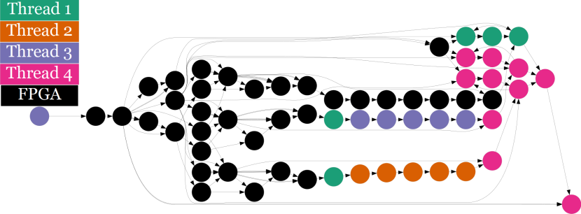
Figure 10: Best performing heterogeneous partition for the RVC-MPEG4SP benchmark.

Multi-objective optimization is a future direction of our work. The constraint-based formulation that we used to solve the partitioning problem can be extended to handle other objectives as well. A common approach is to define the optimization metric as a linear combination of individual objectives. Concretely, if it is desired to minimize execution time and FPGA resource usage simultaneously, we can minimize $T+\alpha R$, where $T$ is execution time, $R$ is the resource utilization and $\alpha$ is a scaling factor that assigns a relative weight to the objectives.

V-D Exploration Time

There are three stages in our design space exploration methodology: (i) profiling, (ii) solving the MILP formulation, and (iii) evaluating through synthesis and implementation. Not surprisingly, most of the time is spent in the last step.

With the current FPGA tools, synthesis and implementation time takes up to several hours. In our experiments with the U250 board and Vitis 2020.1 tool chain, each heterogeneous point in the Fig. 7a and 9a required 3-5 hours to compile—essentially a week of compilation for each benchmark.

Fortunately, all of points discovered by the MILP formulation can be compiled in parallel. In this evaluation, we distributed compilation to three 24-core (48-thread) servers with 256 GiB of RAM, which enabled us to compile 20 points concurrently (before running out of memory), essentially turning a week into a single day.

Hardware profiling time is highly dependent on the actor network and the input size. In both benchmarks, we used down-sampled inputs to keep the profiling time below 1 hour. Software profiling, on the other hand, takes only seconds.

We use a fast industrial MILP solver and constrained the run time to be less than 5 minutes per core configuration (e.g., 40 minutes with 8 cores). We plan to evaluate an open-source solver back-end as well.

VI Conclusion

This work presents a new dataflow compiler for FPGA-based heterogeneous platforms. With the Cal programming language and its efficient translation to the actor machine model and with our compiler, it is possible to express and compile complex streaming programs for both software and hardware targets. Seamless hardware-software execution of streaming functions written in a single source language opens up new avenues in the design space exploration of a heterogeneous application. In addition, automated partitioning significantly reduces the manual effort required to rewrite and optimize complex programs.

We described how the StreamBlocks compiler generates and interconnects the computation on software and hardware heterogeneous platforms. Moreover, the StreamBlocks partitioning tool uses profiling information to efficiently map the computations onto both software or hardware. Our experiments demonstrate this approach’s potential by exploring multiple partitionings of two large programs.

Our future work includes 1) platform-specific code optimization such as automated HLS directive injection and post-partitioning optimization and 2) multi-objective design space exploration.

VII Appendix

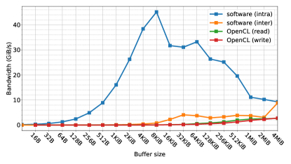
(a)

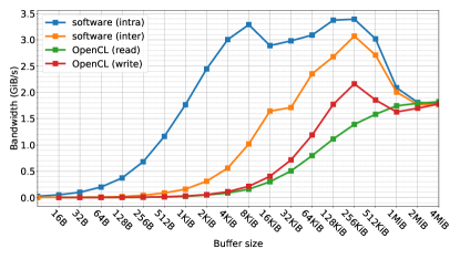
(b)

Figure 11: Measured FIFO communication bandwidth on (a) Alveo U250 and (b) ZCU106.

VII-A MILP Formulation Details

$T_{plink}^{write}$ and $T_{plink}^{read}$ are upper bound estimates of the runtime cost of transferring data between host and FPGA. We represent the set of all connection as the set $C$ and such that $(s,t)\in C$ denotes a connection from source port $s$ to target port $t$. Furthermore, $s.a$ and $t.a$ denote the actor that the port belongs to.

We obtain the number of tokens traversed a connection $(s,t)$ through profiling and denote it as $n_{(s,t)}$. Every connection also has an associated buffer size $b_{(s,t)}$. OpenCL read and write operations are most efficient if a full buffer (i.e., $b_{(s,t)}$ tokens) are transferred.

We measured the OpenCL transfer operation times from queueing to completion using OpenCL event counters to obtain a function $\xi_{r}(b)$ and $\xi_{w}(b)$ that models OpenCL read and write time given a buffer configuration $b$. Using this function we can estimate the best case time required to write $n$ tokens over buffers with capacity $b$ as:

$$\tau_{w}(n,b)=\begin{cases}\xi_{w}(n)&n\leq b\\ \xi_{w}(b)\times\lfloor\frac{n}{b}\rfloor+\xi_{w}(n\bmod{b})&n>b\end{cases}$$ (4)

Here, $\lfloor.\rfloor$ and $mod$ are the floor and modulo operators. To estimate read times, a function $\tau_{r}(n,b)$ is similarly defined by replacing $\xi_{w}(b)$ with $\xi_{r}(b)$. Now we can estimate PLink read and write times as follows:

$$\begin{split}T_{plink}^{write}=&\sum_{(s,t)\in C}(\neg d^{s.a}_{accel}\land d^{t.a}_{accel})\tau_{w}(n_{(s,t)},b_{(s,t)})\\ T_{plink}^{read}=&\sum_{(s,t)\in C}(d^{s.a}_{accel}\land\neg d^{t.a}_{accel})\tau_{r}(n_{(s,t)},b_{(s,t)})\end{split}$$ (5)

Where $\land$ and $\neg$ are the logical conjunction and negation operators respectively. The conjunction expressions ensure that read and write times are only accounted for connections with one port on the FPGA and the other on the CPU.

Similarly, for every partition $p\in P_{thread}$, we define

$$t^{p}_{intra}=\sum_{(s,t)\in C}(d^{s.a}_{p}\land d^{t.a}_{p})\tau_{intra}(n_{(s,t)},b_{(s,t)})$$ (6)

Where $\tau_{intra}$ is models the intra-core communication time and is obtained by profiling software FIFO read and write bandwidth. To do this, we measure the roundtrip times of sending a token from one port and receiving in from another port going through a pass-through actor. Therefore, we use the same bandwidth value for both read and write (i.e., time for read or write is round-trip time divided by 2).

However, notice that if a connection $(s,t)$ has its source actor on the first partition (i.e., $p_{1}$ which also contains the PLink) and its target actor is on the FPGA, the data should first be copied to the PLink and then to the device. This can be modeled by $t^{plink}_{intra}$ as follows:

$$\begin{split}t^{plink}_{intra}&=\\ \sum_{(s,t)\in C}\left((d^{s.a}_{p_{1}}\land d^{t.a}_{accel})\lor(d^{s.a}_{accel}\right.&\left.\land d^{t.a}_{p_{1}})\right)\tau_{intra}(n_{(s,t)},b_{(s,t)})\end{split}$$ (7)

Where $\lor$ is the logical disjunction operator. We can now define the local core communication cost for each partition $p\in P_{thread}$ as:

$$T^{p}_{intra}=\begin{cases}t^{p}_{intra}&p\in P_{thread}\setminus\{p_{1}\}\\ t^{p}_{intra}+t^{plink}_{intra}&p=p_{1}\end{cases}$$ (8)

Since all the threads operate in parallel, then the total intra-core communication time is obtained as the maximum of individual ones:

$$T_{intra}=max(\{T_{intra}^{p}:p\in P_{thread}\})$$ (9)

Finally, we estimate the core to core communication cost as follows:

$$T_{inter}=\sum_{(s,t)\in C}\Biggl{(}\Biggr{.}\\ \sum_{q\in P_{thread}\setminus\{p_{1}\}}\left(\left((d^{s.a}_{p_{1}}\lor d^{s.a}_{accel})\land d_{q}^{t.a}\right)\lor\right.\\ \left.\left(d_{q}^{s.a}\land(d^{t.a}_{p_{1}}\lor d^{t.a}_{accel})\right)\right)\\ +\sum_{p\in P_{thread}\setminus\{p_{1}\}}\sum_{q\in P_{thread}\setminus\{p,p_{1}\}}\left(\left(d^{s.a}_{p}\land d^{t.a}_{q}\right)\lor\left(d^{s.a}_{q}\land d^{t.a}_{p}\right)\right)\\ \Biggl{.}\Biggr{)}\tau_{inter}(n_{(s,t)},b_{(s,t)})$$ (10)

This formula includes a cost for all of the connection that cross a thread. Notice how the first partition $p_{1}$ which contains the PLink is treated slightly differently to handle connections from a thread $q\neq p_{1}$ to $accel$ or $p_{1}$ and vice versa.

With the derivation of $T_{inter}$, $T_{intra}$ and $T_{plink}^{read}$ and $T_{plink}^{write}$ our formulation is complete.

VII-B MILP Model Accuracy

The MILP formulation is a crude and optimistic model for performance. It tries to model a data-dependent and dynamic system with a series of linear equations. To better understand the quality of our modelling, we first describe its sources of inaccuracy.

1. Assuming perfect dataflow The hardware and multi-threaded execution times (excluding communication cost) is modeled as the maximum of individual hardware actor and software thread execution times respectively (see Section III-F). This oversimplified model then inherently disregards any data-dependent behavior and assumes a perfect task-pipelined execution on hardware and no data-starvation on software.

2. Assuming perfect transfers The communication cost model included in the appendix assumes that the FIFOs in software and those that cross the PCIe bus operate at full efficiency. This means our model does not capture executions in which data-dependence leads to poor communication efficiency. In fact, in Fig. 9a there are 3 heterogeneous points that perform poorly. In the single-core heterogeneous point at the lower left of the Fig. 9a, on average 25.12 OpenCL kernel calls are made to decode 10 frames while for the best heterogeneous point (which uses 4 threads) this number is 1.9 OpenCL kernel calls. We have also measured the runtime bandwidth of the output ports of the poorly performing configuration using OpenCL event counters and observed that the PCIe bus was underutilized. Notice that such discrepancies between our model leads to design points with undesirable quality.

3. Profiling errors The $exec(\_,\_)$ and $\xi(\_)$ functions in the formulation come from profiling which entails some inherent error from measurement.

4. Clock period approximation When solving the MILP, we should ”guess” a final operating frequency for the FPGA, and assume a ”fixed” clock speed for the host. The compiled FPGA bitsream may end up operating at a clock speed different from the guessed value and the fixed clock speed can not capture the effects of frequency scaling present on the host.

Considering all of the possible sources of errors described, the end-to-end median execution time prediction accuracy for RVC-MPEG4SP is 22.66% in Fig. 9a and 20.294% in Fig. 9b. The JPEG Blur benchmarks has a 12.84% median error in Fig. 7a on Alveo and a 34.03% median error in Fig. 7b on ZCU106.

Simulation can model data-dependent behavior and therefore will give better performance prediction than “static formulation” but simulating a single design point can take hours. An effective design space exploration would require exploring not one, but maybe tens to hundreds of points which makes simulation unattractive.

VII-C Communication Cost Measurements

In the MILP formulation, the communication cost is parameterized as a function $\xi(b)$ that represents the measured read or write times. If we plot the communication bandwidth as $b/\xi(b)$, then we obtain the Fig. 11a and Fig. 11b for the Alveo U250 and ZCU106 platforms respectively.

Notice the large difference between inter- and intra-core communication bandwidth in Fig 11a. This is because when the two ends of a FIFO are on the same core (i.e., pinned thread), then the communication goes through the private caches (e.g., L1 and L2) without coherence traffic. When the two ends of a FIFO are on two different cores, the tokens travel at least to the shared last-level cache (i.e., L3), which incurs a coherence cost.

As expected, the intra-core bandwidth increases with larger buffer transfers But there is an inflection point at 4KiB (the L1 data size on x86), and at 8KiB the bandwidth starts to descend.

Furthermore, you can observe that OpenCL read and write operations are considerably slower than software FIFO operations and they only partially catch up around 1MiB.

The communication cost terms in the MILP formulation penalize using too many threads or placing everything in hardware without accounting for the considerable overhead of OpenCL read and write operations or inter-core communication.

References

- [1] Andrew Putnam, Adrian M. Caulfield, Eric S. Chung, Derek Chiou, Kypros Constantinides, John Demme, Hadi Esmaeilzadeh, Jeremy Fowers, Gopi Prashanth Gopal, Jan Gray, and et al., “A reconfigurable fabric for accelerating large-scale datacenter services,” SIGARCH Comput. Archit. News, vol. 42, no. 3, pp. 13–24, June 2014.
- [2] A. M. Caulfield, E. S. Chung, A. Putnam, H. Angepat, J. Fowers, M. Haselman, S. Heil, M. Humphrey, P. Kaur, J. Kim, D. Lo, T. Massengill, K. Ovtcharov, M. Papamichael, L. Woods, S. Lanka, D. Chiou, and D. Burger, “A cloud-scale acceleration architecture,” in 2016 49th Annual IEEE/ACM International Symposium on Microarchitecture (MICRO), Oct 2016, pp. 1–13.
- [3] S. Byma, J. G. Steffan, H. Bannazadeh, A. L. Garcia, and P. Chow, “Fpgas in the cloud: Booting virtualized hardware accelerators with openstack,” in 2014 IEEE 22nd Annual International Symposium on Field-Programmable Custom Computing Machines, May 2014, pp. 109–116.
- [4] J. Weerasinghe, F. Abel, C. Hagleitner, and A. Herkersdorf, “Enabling fpgas in hyperscale data centers,” in 2015 IEEE 12th Intl Conf on Ubiquitous Intelligence and Computing and 2015 IEEE 12th Intl Conf on Autonomic and Trusted Computing and 2015 IEEE 15th Intl Conf on Scalable Computing and Communications and Its Associated Workshops (UIC-ATC-ScalCom), Aug 2015, pp. 1078–1086.
- [5] J. Weerasinghe, R. Polig, F. Abel, and C. Hagleitner, “Network-attached fpgas for data center applications,” in 2016 International Conference on Field-Programmable Technology (FPT), Dec 2016, pp. 36–43.
- [6] Mentor Graphics Inc., “Google develops webm video decompression hardware ip using technology independent sources and high-level synthesis,” White paper, 2015.
- [7] Yongfeng Gu Kiran Kintali and Eric Cigan, “Model-based design using simulink, hdl coder, and dsp builder for intel fpgas,” White paper, Matlab Inc., 2014.
- [8] Sassan Ahmadi, “Toward 5g xilinx solutions and enablers for next-generation wireless systems,” White paper, Xilinx Inc., 2016.
- [9] Xilinx, Vivado Design Suite User Guide - High-Level Synthesis, Xilinx Inc.
- [10] J. Choi, Ruo Long Lian, S. Brown, and J. Anderson, “A unified software approach to specify pipeline and spatial parallelism in fpga hardware,” in 2016 IEEE 27th International Conference on Application-specific Systems, Architectures and Processors (ASAP), July 2016, pp. 75–82.
- [11] J. Eker and J. Janneck, “CAL Language Report,” Tech. Rep. ERL Technical Memo UCB/ERL M03/48, University of California at Berkeley, Dec. 2003.
- [12] Jack B. Dennis, “First version of a data flow procedure language,” in Symposium on Programming, 1974, pp. 362–376.
- [13] Gilles Kahn, “The Semantics of Simple Language for Parallel Programming,” in IFIP Congress, 1974, pp. 471–475.
- [14] E.A. Lee and T.M. Parks, “Dataflow process networks,” Proceedings of the IEEE, vol. 83, no. 5, pp. 773 –801, May 1995.
- [15] G. Bilsen, M. Engels, R. Lauwereins, and J.A. Peperstraete, “Cyclo-static data flow,” in Acoustics, Speech, and Signal Processing, 1995. ICASSP-95., 1995 International Conference on, May 1995, vol. 5, pp. 3255 –3258 vol.5.
- [16] Gustav Cedersjö and Jörn W. Janneck, “Tÿcho: A framework for compiling stream programs,” ACM Trans. Embed. Comput. Syst., vol. 18, no. 6, Dec. 2019.
- [17] E.A. Lee and D.G. Messerschmitt, “Synchronous data flow,” Proceedings of the IEEE, vol. 75, no. 9, pp. 1235–1245, Sept 1987.
- [18] J. T. Buck and E. A. Lee, “Scheduling dynamic dataflow graphs with bounded memory using the token flow model,” in 1993 IEEE International Conference on Acoustics, Speech, and Signal Processing, April 1993, vol. 1, pp. 429–432 vol.1.
- [19] ISO/IEC 23001-4:2011, “Information technology - MPEG systems technologies - Part 4: Codec configuration representation,” 2011.
- [20] J.W. Janneck, “A machine model for dataflow actors and its applications,” in Signals, Systems and Computers (ASILOMAR), 2011 Conference Record of the Forty Fifth Asilomar Conference on, Nov 2011, pp. 756–760.
- [21] G. Cedersjö and J. W. Janneck, “Toward efficient execution of dataflow actors,” in 2012 Conference Record of the Forty Sixth Asilomar Conference on Signals, Systems and Computers (ASILOMAR), Nov 2012, pp. 1465–1469.
- [22] J. Eker, J. W. Janneck, E. A. Lee, Jie Liu, Xiaojun Liu, J. Ludvig, S. Neuendorffer, S. Sachs, and Yuhong Xiong, “Taming heterogeneity - the ptolemy approach,” Proceedings of the IEEE, vol. 91, no. 1, pp. 127–144, 2003.
- [23] J. E. Stone, D. Gohara, and G. Shi, “Opencl: A parallel programming standard for heterogeneous computing systems,” Computing in Science Engineering, vol. 12, no. 3, pp. 66–73, 2010.
- [24] Xilinx, Vitis Unified Software Platform User Documentation: Application Acceleration Development, Xilinx Inc., 2019.2 edition, 2019 2019.
- [25] Jörn Janneck, Ian Miller, David Parlour, Ghislain Roquier, Matthieu Wipliez, and Mickaël Raulet, “Synthesizing Hardware from Dataflow Programs: An MPEG-4 Simple Profile Decoder Case Study,” Journal of Signal Processing Systems, vol. 63, no. 2, pp. 241–249, 2009, 10.1007/s11265-009-0397-5.
- [26] Herve Yviquel, Antoine Lorence, Khaled Jerbi, Gildas Cocherel, Alexandre Sanchez, and Mickael Raulet, “Orcc: Multimedia development made easy,” in Proceedings of the 21st ACM International Conference on Multimedia. 2013, MM ’13, pp. 863–866, ACM.
- [27] E. Bezati, M. Mattavelli, and J.W. Janneck, “High-level synthesis of dataflow programs for signal processing systems,” in Image and Signal Processing and Analysis (ISPA), 2013 8th International Symposium on, Sept 2013, pp. 750–754.
- [28] E. Bezati, S. Casale-Brunet, R. Mosqueron, and M. Mattavelli, “An heterogeneous compiler of dataflow programs for zynq platforms,” in ICASSP 2019 - 2019 IEEE International Conference on Acoustics, Speech and Signal Processing (ICASSP), May 2019, pp. 1537–1541.
- [29] K. Jerbi, M. Raulet, O. Deforges, and M. Abid, “Automatic generation of synthesizable hardware implementation from high level RVC-CAL description,” in Acoustics, Speech and Signal Processing (ICASSP), 2012 IEEE International Conference on, March 2012, pp. 1597–1600.
- [30] N. Siret, M. Wipliez, J.-F. Nezan, and A. Rhatay, “Hardware code generation from dataflow programs,” in Design and Architectures for Signal and Image Processing (DASIP), 2010 Conference on, Oct 2010, pp. 113–120.
- [31] Joachim Falk, Christian Haubelt, Jürgen Teich, and Christian Zebelein, “SysteMoC: A Data-Flow Programming Language for Codesign,” in Handbook of Hardware/Software Codesign, Teich J Ha S, Ed., vol. 1, pp. 59 – 97. Springer, Dordrecht, The Netherlands, 2017.
- [32] Joachim Keinert, Martin Streubūhr, Thomas Schlichter, Joachim Falk, Jens Gladigau, Christian Haubelt, Jūrgen Teich, and Michael Meredith, “SystemCoDesigner—an automatic esl synthesis approach by design space exploration and behavioral synthesis for streaming applications,” ACM Trans. Des. Autom. Electron. Syst., vol. 14, no. 1, Jan. 2009.
- [33] Juan Fumero, Michail Papadimitriou, Foivos S. Zakkak, Maria Xekalaki, James Clarkson, and Christos Kotselidis, “Dynamic application reconfiguration on heterogeneous hardware,” in Proceedings of the 15th ACM SIGPLAN/SIGOPS International Conference on Virtual Execution Environments, New York, NY, USA, 2019, VEE 2019, p. 165–178, Association for Computing Machinery.
- [34] Eric S. Chung, John D. Davis, and Jaewon Lee, “Linqits: Big data on little clients,” in Proceedings of the 40th Annual International Symposium on Computer Architecture, New York, NY, USA, 2013, ISCA ’13, p. 261–272, Association for Computing Machinery.
- [35] Eylon Caspi, Michael Chu, Randy Huang, Joseph Yeh, John Wawrzynek, and André DeHon, “Stream computations organized for reconfigurable execution (SCORE),” in Proceedings of the The Roadmap to Reconfigurable Computing, 10th International Workshop on Field-Programmable Logic and Applications, Berlin, Heidelberg, 2000, FPL ’00, p. 605–614, Springer-Verlag.
- [36] Simone Casale-Brunet, Abdallah Elguindy, Endri Bezati, Richard Thavot, Ghislain Roquier, Marco Mattavelli, and Jorn W Janneck, “Methods to explore design space for mpeg rmc codec specifications,” Signal Processing: Image Communication, vol. 28, no. 10, pp. 1278–1294, 2013.
- [37] Jason Cong, Peng Li, Bingjun Xiao, and Peng Zhang, “An optimal microarchitecture for stencil computation acceleration based on non-uniform partitioning of data reuse buffers,” in Proceedings of the 51st Annual Design Automation Conference, New York, NY, USA, 2014, DAC ’14, p. 1–6, Association for Computing Machinery.
- [38] S. Casale-Brunet, E. Bezati, and M. Mattavelli, “Design space exploration of dataflow-based smith-waterman fpga implementations,” in 2017 IEEE International Workshop on Signal Processing Systems (SiPS), Oct 2017, pp. 1–6.