\newconstantfamily

Nsymbol=N

Single-exponential bounds for the smallest singular value of Vandermonde matrices in the sub-Rayleigh regime

Dmitry Batenkov Department of Applied Mathematics, School of Mathematical Sciences, Tel Aviv University, P.O. Box 39040, Tel Aviv 6997801, Israel dbatenkov@tauex.tau.ac.il Β andΒ  Gil Goldman Department of Mathematics, The Weizmann Institute of Science, Rehovot 76100, Israel gil.goldman@weizmann.ac.il
Abstract.

Following recent interest by the community, the scaling of the minimal singular value of a Vandermonde matrix with nodes forming clusters on the length scale of Rayleigh distance on the complex unit circle is studied. Using approximation theoretic properties of exponential sums, we show that the decay is only single exponential in the size of the largest cluster, and the bound holds for arbitrary small minimal separation distance. We also obtain a generalization of well-known bounds on the smallest eigenvalue of the generalized prolate matrix in the multi-cluster geometry. Finally, the results are extended to the entire spectrum.

Key words and phrases:
Vandermonde matrices with nodes on the unit circle, nonuniform Fourier matrices, sub-Rayleigh resolution, singular values, super-resolution, condition number.
2010 Mathematics Subject Classification:
Primary 15A18, 65T40, 65F20.
D.B. was supported by the ISRAEL SCIENCE FOUNDATION (grant No. 1793/20)

1. Introduction

For an ordered set of distinct nodes $\mathcal{X}=\{x_{1},\ldots,x_{s}\}$ with $x_{j}\in(-\pi,\pi]$, and $N\geq s-1$, consider the $(N+1)\times s$ Vandermonde matrix

$$\mathbf{V}_{N}(\mathcal{X}):=\left[e^{\imath kx_{j}}\right]_{0\leq k\leq N}^{1\leq j\leq s}.$$ (1.1)

This class of matrices is the subject of numerous recent investigations in the applied harmonic analysis community, e.g. [1, 4, 5, 14, 17, 18, 19, 20, 21, 22]. While interesting in their own right, the spectral properties of $\mathbf{V}_{N}$ are closely related to the problem of super-resolution (SR) under sparsity constraints, which also received a lot of attention in recent years [6, 8, 9, 11]. In the SR context, the smallest singular value $\sigma_{\min}(\mathbf{V}_{N}):=\min_{\boldsymbol{\mathrm{c}}\in\mathbb{C}^{s},\|\boldsymbol{\mathrm{c}}\|_{2}=1}\|\mathbf{V}_{N}\boldsymbol{\mathrm{c}}\|_{2}$ controls the limit of stable recovery of a superposition of Dirac masses supported on $\mathcal{X}$ from its first $N+1$ Fourier coefficients, while the singular subspaces play a major role in various SR algorithms (e.g. MUSIC and ESPRIT) [13, 19, 20, 21].

Let $\Delta$ denote the minimal separation (in the wrap-around sense) between the elements of $\mathcal{X}$. With $s$ fixed, two distinct asymptotic regimes are known:

  1. (1)

    When $N\Delta\gtrapprox O(1)$, the matrix $\mathbf{V}_{N}$ is well-conditioned, and $\sigma_{\min}(\mathbf{V}_{N})=O(\sqrt{N})$.

  2. (2)

    When $N\Delta\ll 1$, $\sigma_{\min}(\mathbf{V}_{N})$ can be as small as $O\left(\sqrt{N}(N\Delta)^{s-1}\right)$.

The well-conditioned case 1) has been studied in [1, 16, 22, 23, 25], by various tools from harmonic analysis and analytic number theory. The separation condition $\Delta\gtrapprox{1\over N}$ plays a major role in the analysis of the convex relaxations of the SR problem [7, 8].

Case 2) corresponds to the so-called β€œsub-Rayleigh” regime, where $N=2\pi\Delta^{-1}$ is precisely the Rayleigh resolution limit. The possibility to resolve closely spaced point sources from low-frequency measurements with arbitrary precision was already established by G.Β deΒ Prony in 1795 [26]111English translation of the original Prony’s paper can be found in [2]., providing the symbolic-algebraic basis for many other reconstruction algorithms that followed. However, without additional prior information regarding the geometry of $\mathcal{X}$, the sensitivity to noise (β€œcondition number”) of the SR problem in the sub-Rayleigh regime may be as large as $\operatorname{SRF}^{2s-1}$, where $\operatorname{SRF}:=(N\Delta)^{-1}$ is the β€œsuper-resolution factor”. This quickly becomes prohibitive already for moderate values of $s$. The exponent $2s-1$ corresponds to the worst-case scenario where all the nodes of $\mathcal{X}$ are clustered together and approximately equispaced, e.g. $x_{j+1}=x_{j}+\Delta_{j}$ with $\Delta_{j}\approx\Delta$, $j=1,\dots,s-1$.

When $\Delta_{j}=\Delta$ for all $1\leq j\leq s-1$, $\mathbf{V}_{N}$ is a contiguous submatrix of the DFT matrix (also known as the β€œprolate matrix” in the literature [29]), and the scaling of $\sigma_{\min}(\mathbf{V}_{N})$, in the asymptotic regime $N\to\infty,\;N\Delta<c$ directly follows from the β€œBell Labs theory” of the spectral concentration problem [27] (see also [3]). See Section 3 for further discussion.

Now suppose that an a-priori information is available, according to which only a small number of nodes can be clustered, with the different clusters separated by $\theta\gtrapprox{1\over N}$ (see Definition 2.3 below). It has been recently shown by several groups that in this case, $\sigma_{\min}(\mathbf{V}_{N})\asymp\sqrt{N}(N\Delta)^{\ell-1}$ where $\ell$ is the largest multiplicity of any such cluster. Accordingly, the SR condition number will scale as $\operatorname{SRF}^{2\ell-1}$ [4, 5, 6, 10, 17, 18, 19].

The scaling of the proportionality constants in the order estimates above, in particular, their dependence on $\ell$ and $s$, are a subject of ongoing research. This question is of importance in the regime where $\ell\ll s$, so that the factor $\operatorname{SRF}^{2\ell-1}$ is significantly smaller than $\operatorname{SRF}^{2s-1}$.

In this paper we prove a single-exponential in $\ell$ and linear in $s$ lower bound for $\sigma_{\min}(\mathbf{V}_{N}(\mathcal{X}))$ in the multi-cluster geometry (Theorem 2.2), of the form

$$\sigma_{\min}(\mathbf{V}_{N}(\mathcal{X}))\geq c_{1}\sqrt{N}(N\Delta/c_{2})^{\ell-1},$$ (1.2)

where $c_{1},c_{2}$ are absolute constants, independent of $\ell,s,N,\Delta$, (and in fact, $c_{2}=32\pi e$), holding whenever

c3​(β„“)​s/θ≀N≀c4​(β„“)/(τ​Δ​s).subscript𝑐3β„“π‘ πœƒπ‘subscript𝑐4β„“πœΞ”π‘ c_{3}(\ell)s/\theta\leq N\leq c_{4}(\ell)/(\tau\Delta s). (1.3)

Relative to prior works on the subject, in particular [18, 19] (see Section 3 below), our single-exponential in $\ell$ bound (1.2) holds for a fixed $N$ and all sufficiently small $\Delta$. Applying a simple limiting argument, in Theorem 2.3 we also generalize Slepian’s bound for the smallest eigenvalue of the prolate matrix (see above) in the non-equispaced multi-cluster case.

The main technical contribution of this paper is a new method of proof of the bound (1.2) for a single cluster (Theorem 2.1), which was previously shown in this setting in [18, Example 4.8] (again, see details in Section 3). The proof is based on applying the classical Turan’s inequality for exponential sums and Salem’s inequality to the analysis of stability of Vandermonde matrices with nodes on the unit circle. The extension of this result to Vandermonde matrices with multiple sets of clustered nodes separated by $\theta\gtrsim{1\over N}$, is done by invoking our recent result [5, Theorem 2.2], which, in turn, shows that the column subspaces in $\mathbb{C}^{N+1}$ corresponding to each cluster are nearly orthogonal.

Our results can easily be extended to show single-exponential scaling for all the singular values of $\mathbf{V}_{N}$ (resp. eigenvalues of the prolate matrix). We present some details of these extensions in Section 7, however for the sake of brevity we do not provide the full derivations.

2. Main results

Definition 2.1 (Wrap-around distance).

For $x,y\in\mathbb{R}$, we define the wrap-around distance

$$d(x,y):=\bigl{|}\operatorname{Arg}\exp{\imath(x-y)}\bigr{|}=\bigl{|}x-y\mod(-\pi,\pi]\bigr{|}\in\left[0,\pi\right],$$

where for $z\in{\mathbb{C}}\backslash\{0\}$, $\operatorname{Arg}(z)$ is the principal value of the argument of $z$, taking values in $\left(-\pi,\pi\right]$.

We denote by $\mathbb{T}=\mathbb{R}\mod(-\pi,\pi]$ the periodic interval of length $2\pi$.

Definition 2.2 (Single cluster configuration).

The node set $\mathcal{X}=\left\{x_{1},\dots,x_{\ell}\right\}\subset(-\pi,\pi]$ is said to form a $(\Delta,\ell,\tau)_{\mathbb{T}}$-cluster, for some $\ell-1\leq\tau\leq{\pi\over\Delta}$, if

βˆ€x,yβˆˆπ’³,xβ‰ y:Δ≀d(x,y)≀τΔ.\forall x,y\in\mathcal{X},x\neq y:\quad\Delta\leq d(x,y)\leq\tau\Delta.

Below we write $C_{k}(\ell)$, for some indexes $k=1,\ldots$, to indicate constants that depend only on $\ell$.

Our first main result is the following.

Theorem 2.1.

Let $\mathcal{X}$ form a $(\Delta,\ell,\tau)_{\mathbb{T}}$-clustered configuration. Then there exist a constant \Cl​s​i​n​g​l​e.c​l​u​s​t​e​r.N​(β„“)formulae-sequence\Clπ‘ π‘–π‘›π‘”π‘™π‘’π‘π‘™π‘’π‘ π‘‘π‘’π‘Ÿπ‘β„“\Cl{single.cluster.N}(\ell) and absolute constants \Cl​s​i​n​g​l​e.c​l​u​s​t​e​r.l​o​w​e​r=32​π​e,\Cl​s​i​n​g​l​e.c​l​u​s​t​e​r.m​u​l​tformulae-sequence\Clπ‘ π‘–π‘›π‘”π‘™π‘’π‘π‘™π‘’π‘ π‘‘π‘’π‘Ÿπ‘™π‘œπ‘€π‘’π‘Ÿ32πœ‹π‘’\Clπ‘ π‘–π‘›π‘”π‘™π‘’π‘π‘™π‘’π‘ π‘‘π‘’π‘Ÿπ‘šπ‘’π‘™π‘‘\Cl{single.cluster.lower}=32\pi e,\Cl{single.cluster.mult}, such that for any $N$ satisfying \Cr​s​i​n​g​l​e.c​l​u​s​t​e​r.N​(β„“)≀N≀2​πτ​Δformulae-sequence\Crπ‘ π‘–π‘›π‘”π‘™π‘’π‘π‘™π‘’π‘ π‘‘π‘’π‘Ÿπ‘β„“π‘2πœ‹πœΞ”\Cr{single.cluster.N}(\ell)\leq N\leq\frac{2\pi}{\tau\Delta},

$$\sigma_{\min}(\mathbf{V}_{N}(\mathcal{X})))\geq\Cr{single.cluster.mult}\sqrt{N}\biggl{(}\frac{N\Delta}{\Cr{single.cluster.lower}}\biggr{)}^{\ell-1}.$$ (2.1)
Definition 2.3 (Multi-cluster configuration, periodic interval).

The node set 𝒳={x1,…,xs}βŠ‚(βˆ’Ο€,Ο€]𝒳subscriptπ‘₯1…subscriptπ‘₯π‘ πœ‹πœ‹\mathcal{X}=\left\{x_{1},\dots,x_{s}\right\}\subset(-\pi,\pi] is said to form a (Ξ”,ΞΈ,s,β„“,Ο„)𝕋subscriptΞ”πœƒπ‘ β„“πœπ•‹\left(\Delta,\theta,s,\ell,\tau\right)_{\mathbb{T}}-clustered configuration for some $\Delta>0$, $1\leq\ell\leq s$, $\ell-1\leq\tau\leq{\pi\over\Delta}$ and $\theta>0$, if for each $x_{j}$, there exist at most $\ell$ distinct nodes

$$\mathcal{X}^{(j)}=\{x_{j,k}\}_{k=1,\dots,r_{j}}\subset\mathcal{X},\;1\leq r_{j}\leq\ell,\quad x_{j,1}\equiv x_{j},$$

such that the following conditions are satisfied:

  1. (1)

    For any $y\in\mathcal{X}^{(j)}\setminus\{x_{j}\}$, we have

    $$\Delta\leq d(y,x_{j})\leq\tau\Delta.$$
  2. (2)

    For any $y\in\mathcal{X}\setminus\mathcal{X}^{(j)}$, we have

    $$d(y,x_{j})\geq\theta.$$
Theorem 2.2.

There exist constants \Cl​m​u​l​t​i.c​l​u​s​t​e​r.N.t​h​e​t​a​(β„“)formulae-sequence\Clπ‘šπ‘’π‘™π‘‘π‘–π‘π‘™π‘’π‘ π‘‘π‘’π‘Ÿπ‘π‘‘β„Žπ‘’π‘‘π‘Žβ„“\Cl{multi.cluster.N.theta}(\ell), \Cl​m​u​l​t​i.c​l​u​s​t​e​r.N.d​e​l​t​a​(β„“)formulae-sequence\Clπ‘šπ‘’π‘™π‘‘π‘–π‘π‘™π‘’π‘ π‘‘π‘’π‘Ÿπ‘π‘‘π‘’π‘™π‘‘π‘Žβ„“\Cl{multi.cluster.N.delta}(\ell) and absolute constants \Cl​m​u​l​t​i.c​l​u​s​t​e​r.l​o​w​e​r.i​n=32​π​e,\Cl​m​u​l​t​i.c​l​u​s​t​e​r.m​u​l​tformulae-sequence\Clπ‘šπ‘’π‘™π‘‘π‘–π‘π‘™π‘’π‘ π‘‘π‘’π‘Ÿπ‘™π‘œπ‘€π‘’π‘Ÿπ‘–π‘›32πœ‹π‘’\Clπ‘šπ‘’π‘™π‘‘π‘–π‘π‘™π‘’π‘ π‘‘π‘’π‘Ÿπ‘šπ‘’π‘™π‘‘\Cl{multi.cluster.lower.in}=32\pi e,\Cl{multi.cluster.mult}, such that for any $\mathcal{X}$ forming a (Ξ”,ΞΈ,s,β„“,Ο„)𝕋subscriptΞ”πœƒπ‘ β„“πœπ•‹\left(\Delta,\theta,s,\ell,\tau\right)_{\mathbb{T}}-clustered configuration and $N$ satisfying \Cr​m​u​l​t​i.c​l​u​s​t​e​r.N.t​h​e​t​a​sθ≀N≀\Cr​m​u​l​t​i.c​l​u​s​t​e​r.N.d​e​l​t​as​τ​Δformulae-sequence\Crπ‘šπ‘’π‘™π‘‘π‘–π‘π‘™π‘’π‘ π‘‘π‘’π‘Ÿπ‘π‘‘β„Žπ‘’π‘‘π‘Žπ‘ πœƒπ‘formulae-sequence\Crπ‘šπ‘’π‘™π‘‘π‘–π‘π‘™π‘’π‘ π‘‘π‘’π‘Ÿπ‘π‘‘π‘’π‘™π‘‘π‘Žπ‘ πœΞ”\frac{\Cr{multi.cluster.N.theta}s}{\theta}\leq N\leq\frac{\Cr{multi.cluster.N.delta}}{s\tau\Delta},

$\displaystyle\sigma_{\min}\left(\mathbf{V}_{N}\left(\mathcal{X}\right)\right)$ β‰₯\Cr​m​u​l​t​i.c​l​u​s​t​e​r.m​u​l​t​N​(N​Δ\Cr​m​u​l​t​i.c​l​u​s​t​e​r.l​o​w​e​r.i​n)β„“βˆ’1.formulae-sequenceabsent\Crπ‘šπ‘’π‘™π‘‘π‘–π‘π‘™π‘’π‘ π‘‘π‘’π‘Ÿπ‘šπ‘’π‘™π‘‘π‘superscript𝑁Δformulae-sequence\Crπ‘šπ‘’π‘™π‘‘π‘–π‘π‘™π‘’π‘ π‘‘π‘’π‘Ÿπ‘™π‘œπ‘€π‘’π‘Ÿπ‘–π‘›β„“1\displaystyle\geq\Cr{multi.cluster.mult}\sqrt{N}\left(\frac{N\Delta}{\Cr{multi.cluster.lower.in}}\right)^{\ell-1}. (2.2)
Definition 2.4 (Generalized prolate matrix).

Let $\mathcal{X}=\left\{x_{1},\dots,x_{s}\right\}\subset\mathbb{R}$ be a collection of $s$ pairwise distinct points on the real line. We define the generalized prolate matrix as follows:

$$\mathbf{G}(\mathcal{X})=\biggl{[}\frac{1}{2}\int_{-1}^{1}e^{\imath\omega(x_{j}-x_{k})}\biggr{]}_{j,k=1}^{s}\in\mathbb{R}^{s\times s}.$$

Note that $\mathbf{G}(\mathcal{X})$ is symmetric and positive definite (see e.g. [4, Proposition 2.6]).

In a manner completely analogous to Definition 2.2, we define the notion of a clustered configuration appropriate for this setting.

Definition 2.5 (Multi-cluster configuration, real line).

The node set $\mathcal{X}=\left\{x_{1},\dots,x_{s}\right\}\subset\mathbb{R}$ is said to form a (Ξ”,ΞΈ,s,β„“,Ο„)ℝsubscriptΞ”πœƒπ‘ β„“πœβ„\left(\Delta,\theta,s,\ell,\tau\right)_{\mathbb{R}}-clustered configuration for some $\Delta>0$, $1\leq\ell\leq s$, $\ell-1\leq\tau$ and $\theta>0$, if for each $x_{j}$, there exist at most $\ell$ distinct nodes

$$\mathcal{X}^{(j)}=\{x_{j,k}\}_{k=1,\dots,r_{j}}\subset\mathcal{X},\;1\leq r_{j}\leq\ell,\quad x_{j,1}\equiv x_{j},$$

such that the following conditions are satisfied:

  1. (1)

    For any $y\in\mathcal{X}^{(j)}\setminus\{x_{j}\}$, we have

    $$\Delta\leq\left|y-x_{j}\right|\leq\tau\Delta.$$
  2. (2)

    For any $y\in\mathcal{X}\setminus\mathcal{X}^{(j)}$, we have

    $$\left|y-x_{j}\right|\geq\theta.$$

The next theorem is a direct corollary of Theorem 2.2, and it should be compared to (3.1).

Theorem 2.3.

There exist absolute constants \Cl​m​u​l​t​i.c​l​u​s​t​e​r.p​r​o​l​a​t​e.l​o​w​e​rformulae-sequence\Clπ‘šπ‘’π‘™π‘‘π‘–π‘π‘™π‘’π‘ π‘‘π‘’π‘Ÿπ‘π‘Ÿπ‘œπ‘™π‘Žπ‘‘π‘’π‘™π‘œπ‘€π‘’π‘Ÿ\Cl{multi.cluster.prolate.lower}, \Cl​m​u​l​t​i.c​l​u​s​t​e​r.l​o​w​e​r.O=16​π​eformulae-sequence\Clπ‘šπ‘’π‘™π‘‘π‘–π‘π‘™π‘’π‘ π‘‘π‘’π‘Ÿπ‘™π‘œπ‘€π‘’π‘Ÿπ‘‚16πœ‹π‘’\Cl{multi.cluster.lower.O}=16\pi e and constants \Cl​m​u​l​t​i.c​l​u​s​t​e​r.O.t​h​e​t​a​(β„“)formulae-sequence\Clπ‘šπ‘’π‘™π‘‘π‘–π‘π‘™π‘’π‘ π‘‘π‘’π‘Ÿπ‘‚π‘‘β„Žπ‘’π‘‘π‘Žβ„“\Cl{multi.cluster.O.theta}(\ell), \Cl​m​u​l​t​i.c​l​u​s​t​e​r.O.d​e​l​t​a​(β„“)formulae-sequence\Clπ‘šπ‘’π‘™π‘‘π‘–π‘π‘™π‘’π‘ π‘‘π‘’π‘Ÿπ‘‚π‘‘π‘’π‘™π‘‘π‘Žβ„“\Cl{multi.cluster.O.delta}(\ell), such that for any $\mathcal{X}$ forming a (Ξ”,ΞΈ,s,β„“,Ο„)ℝsubscriptΞ”πœƒπ‘ β„“πœβ„\left(\Delta,\theta,s,\ell,\tau\right)_{\mathbb{R}}-clustered configuration with ΞΈβ‰₯\Cr​m​u​l​t​i.c​l​u​s​t​e​r.O.t​h​e​t​a​sformulae-sequenceπœƒ\Crπ‘šπ‘’π‘™π‘‘π‘–π‘π‘™π‘’π‘ π‘‘π‘’π‘Ÿπ‘‚π‘‘β„Žπ‘’π‘‘π‘Žπ‘ \theta\geq\Cr{multi.cluster.O.theta}s and s​τ​Δ≀\Cr​m​u​l​t​i.c​l​u​s​t​e​r.O.d​e​l​t​aformulae-sequenceπ‘ πœΞ”\Crπ‘šπ‘’π‘™π‘‘π‘–π‘π‘™π‘’π‘ π‘‘π‘’π‘Ÿπ‘‚π‘‘π‘’π‘™π‘‘π‘Žs\tau\Delta\leq\Cr{multi.cluster.O.delta},

$\displaystyle\lambda_{\min}\left(\mathbf{G}\left(\mathcal{X}\right)\right)$ β‰₯\Cr​m​u​l​t​i.c​l​u​s​t​e​r.p​r​o​l​a​t​e.l​o​w​e​r​(Ξ”\Cr​m​u​l​t​i.c​l​u​s​t​e​r.l​o​w​e​r.O)2​(β„“βˆ’1).formulae-sequenceabsent\Crπ‘šπ‘’π‘™π‘‘π‘–π‘π‘™π‘’π‘ π‘‘π‘’π‘Ÿπ‘π‘Ÿπ‘œπ‘™π‘Žπ‘‘π‘’π‘™π‘œπ‘€π‘’π‘ŸsuperscriptΞ”formulae-sequence\Crπ‘šπ‘’π‘™π‘‘π‘–π‘π‘™π‘’π‘ π‘‘π‘’π‘Ÿπ‘™π‘œπ‘€π‘’π‘Ÿπ‘‚2β„“1\displaystyle\geq\Cr{multi.cluster.prolate.lower}\left(\frac{\Delta}{\Cr{multi.cluster.lower.O}}\right)^{2(\ell-1)}. (2.3)
Remark 2.1.

Frequently the definition of the prolate matrix contains an additional bandwidth parameter $\Omega>0$, so that the inner products are considered in an interval $[-\Omega,\Omega]$ [4]. In the present paper we do not lose any generality by rescaling $\Omega$ to 1.

3. Prior art

In this section only, $c,c_{1},\dots,c^{\prime},\dots,C,\dots$ denote generic constants which might be different in different formulas, and which do not depend on $N,\Delta$.

Let us start with the setting $\ell=s$. Recalling Definition 2.4, we have, as $N\to\infty$, that

$$(2N)^{-1}\sigma_{\min}^{2}\left(\mathbf{V}_{N}(\mathcal{X}/N)\right)\to\lambda_{\min}\left(\mathbf{G}(\mathcal{X})\right).$$

In the equispaced setting $x_{j+1}=x_{j}+\Delta$, $j=1,\dots,s-1$, the matrix $\mathbf{G}$ is precisely the β€œprolate matrix” [27, 29], and it holds that

$$\begin{split}\lambda_{\min}(\mathbf{G}(\mathcal{X}))&=C_{EQ}(s)\Delta^{2s-2}\left\{1+O(\Delta)\right\},\quad\Delta\ll 1;\\ C_{EQ}(s)&:=\frac{2^{2s-2}}{(2s-1){2s-2\choose s-1}^{3}}\asymp_{s}\left(1\over 4\right)^{2s-2}.\end{split}$$ (3.1)

Here $\asymp_{s}$ means β€œup to polynomial in $s$ and $1/s$ factors”. This gives

$$\sigma_{\min}(\mathbf{V}_{N})\asymp_{s}\sqrt{N}\biggl{(}\frac{N\Delta}{4}\biggr{)}^{s-1}\left\{1+O(\sqrt{N\Delta})\right\}.$$

Non-asymptotic bounds for the case of node configurations $\mathcal{X}$ with minimal separation of at least $\Delta$ are available as well. An explicit construction in [19, Proposition 3] (following [11]) gives

$$\min_{\mathcal{X}}\sigma_{\min}(\mathbf{V}_{N}(\mathcal{X}))\lessapprox_{s}\sqrt{N}\biggl{(}\frac{N\Delta}{2}\biggr{)}^{s-1},\quad N\Delta<\frac{2\pi}{{C}_{LL}(s)\sqrt{N}},\quad{C}_{LL}(s)=2\pi\sum_{j=0}^{s-1}{s-1\choose j}\frac{j^{s}}{s!}.$$

For a single cluster setting $\ell=s$, Theorem 2.1 has been proven in [18, Example 4.8] with the better constant \Cr​s​i​n​g​l​e.c​l​u​s​t​e​r.l​o​w​e​r=4​π​eformulae-sequence\Crπ‘ π‘–π‘›π‘”π‘™π‘’π‘π‘™π‘’π‘ π‘‘π‘’π‘Ÿπ‘™π‘œπ‘€π‘’π‘Ÿ4πœ‹π‘’\Cr{single.cluster.lower}=4\pi e (in the earlier work [19] this constant was not explicit). The reduction in the tightness of constant in our work might be related to the fact that our constant is also valid for all the singular values, see Theorem 7.1 below.

Turning to the more general case $\ell\leq s$ and cluster separation $\theta$ (as in Definition 2.3), in [19] and later [18, Corollary 4.2] it was shown that

$$\sigma_{\min}(\mathbf{V}_{N}(\mathcal{X}))\geq\frac{5}{9}\sqrt{N}\biggl{(}\frac{N\Delta}{4\pi e}\biggr{)}^{\ell-1},\quad N\Delta<1.$$

However, the above holds under the condition $N\theta>c_{\gamma}(N\Delta)^{-\gamma}$ with any $\gamma>0$ and $c_{\gamma}\to\infty$ as $\gamma\to 0$. For fixed $N,\theta$, this prevents $\Delta\to 0$ in order for the bound to continue to hold. In contrast, assuming $N\theta>c^{\prime}$ and $N\Delta<c^{\prime\prime}$ with $c^{\prime},c^{\prime\prime}$ depending only on $s,\ell$, it was shown in [5, Theorem 2.3, Corollary 2.1] that for all $\mathcal{X}$ satisfying the clustering geometric assumptions, we have

$$C^{\prime}\sqrt{N}(N\Delta)^{\ell-1}\leq\sigma_{\min}(\mathbf{V}_{N}(\mathcal{X}))\leq\frac{1}{2}\sqrt{N\ell e}(\tau N\Delta)^{\ell-1}.$$ (3.2)

Here $\tau\geq(\ell-1)$ is a uniformity parameter, controlling the overall extent of any cluster (see Definition 2.3). However, the constant $C^{\prime}$ was not explicit. In [4] the same scaling for the lower bound was shown with $C^{\prime}=\frac{\sqrt{\pi/2}}{(s\sqrt{2\pi})^{2s-1}}$, albeit under the additional assumption that $x_{j}\in\frac{\pi}{2s^{2}}(-1,1]$ for all $j=1,\dots,s$.

More details on the above developments are available in [5, Section 1.4], [18, Examples 4.7,4.8], [4, Remarks 3.5,3.7] and [19, Remark 4].

Our single-exponential in $\ell$ bound of Theorem 2.2, which holds for a fixed $N$ and all sufficiently small $\Delta$, thus provides an improvement upon the above mentioned results (except, possibly, for the value of the absolute constant \Cr​m​u​l​t​i.c​l​u​s​t​e​r.l​o​w​e​r.i​nformulae-sequence\Crπ‘šπ‘’π‘™π‘‘π‘–π‘π‘™π‘’π‘ π‘‘π‘’π‘Ÿπ‘™π‘œπ‘€π‘’π‘Ÿπ‘–π‘›\Cr{multi.cluster.lower.in}, see Section 4).

4. Numerical experiments

In this section we estimate the exponential dependence of $\sigma_{\min}(\mathbf{V}_{N}(\mathcal{X}))$ on $\ell$ numerically, by computing

$$\Lambda(\mathcal{X},N):=\sigma_{\min}(\mathbf{V}_{N}(\mathcal{X})/(\sqrt{N}(N\Delta)^{\ell-1}).$$

Varying $\ell,\tau$ and $N,\Delta$ fixed, we expect that

$$(1/c_{2})^{\ell-1}\lessapprox\Lambda(\mathcal{X},N)\lessapprox(1/c_{2}^{\prime})^{\ell-1}.$$

Our theoretical results indicate that the above holds with $c_{2}\leq 16\pi e$ and $c_{2}^{\prime}\geq{1/\tau}$ (see resp. (6.10) and (3.2)).

As can be seen from Fig. 1, both the upper and lower bounds are correct, although the corresponding constants $16\pi e$ and $1/\tau$ are not tight.

Refer to caption
Figure 1. Single cluster - dependence of $\sigma_{\min}$ on $\ell$. We plot $\ell$ vs $\log_{10}\Lambda(\mathcal{X},N)$. $N$ is varying between 60 and 300, $\Delta$ is varying between $10^{-25}$ and $10^{-4}$, while $\ell$ varies from 2 to 40 and $\tau$ varies from $\ell-1$ to $\tau_{\max}=80$. The lower and upper bounds are shown as dashed lines.

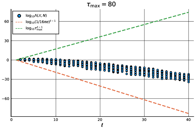
All numerical tests were performed in arbitrary precision arithmetic.

5. Discussion

It is an interesting open question whether a bound of the type (1.2) should hold in the multi-cluster geometry, for $N\theta>c^{\prime},N\Delta<c^{\prime\prime}$ where $c^{\prime},c^{\prime\prime}$ do not depend on $s$ and with no essential further restrictions on $\mathcal{X}$. If this is the case, then it is plausible that the super-resolution problem for a practically infinite spike train ($s\gg 1$) with small sub-Rayleigh clusters (a model analogous to Donoho’s Rayleigh regular measures, [11]) can be essentially decoupled into treating each cluster separately.

There is a room for further refinement regarding the bounds themselves, as there is a relatively large gap in the constants between the upper bound in (3.2) and (1.2).

6. Proofs

6.1. Preliminaries on exponential sums

We review some preliminary results about exponential sums and their implications to the problem at hand.

Definition 6.1.

Given a vector $\boldsymbol{\mathrm{c}}\in\mathbb{C}^{\ell}$ and $\mathcal{X}=\{x_{1},\ldots,x_{\ell}\}\subset\mathbb{R}$, we define the exponential sum

$$P(t)=P_{\boldsymbol{\mathrm{c}},\mathcal{X}}(t):=\sum_{j=1}^{\ell}c_{j}e^{\imath tx_{j}}.$$

The number of nonzero $c_{j}$’s is called the degree of $P$. The set of all exponential sums of degree at most $\ell$ is denoted by $\mathfrak{I}_{\ell}$.

Remark 6.1.

Our definition of exponential sums covers the case of purely imaginary exponents only to simplify the presentation. More general results for arbitrary complex exponents are available in e.g. [24, 12].

We denote by $\mu$ the Lebesgue measure on $\mathbb{R}$.

Given an interval $I$ and a (complex valued) continuous function $f\in C(I)$, $1\leq p\leq\infty$, we denote

$$\|f\|_{L^{p}(I)}:=\begin{cases}\biggl{(}\frac{1}{\mu(I)}\int_{I}|f(t)|^{p}dt\biggr{)}^{1/p},&1\leq p<\infty;\\ \sup_{t\in I}|f(t)|,&p=\infty.\end{cases}$$

Exponential sums satisfy many classical inequalities from approximation theory. In particular, we have the following estimates.

Proposition 6.1 (Turan’s inequality).

Let $P\in\mathfrak{I}_{\ell}$, and let $\Omega\subset I$ be intervals with positive Lebesgue measure. Then

$$\|P\|_{L^{\infty}(I)}\leqslant\left(\frac{4e\mu(I)}{\mu(\Omega)}\right)^{\ell-1}\|P\|_{L^{\infty}(\Omega)}.$$
Proof.

See a review on Turan’s lemma on p.7 of [24] (and Turan’s original result [28], in German).

∎

Proposition 6.2 (Nikolskii-type inequality).

Let $P\in\mathfrak{I}_{\ell}$, then

$$\|P\|_{L^{p}[0,1]}\leqslant\left(\frac{\pi\ell}{2}\right)^{2/q-2/p}\|P\|_{L^{q}[0,1]},\quad 0<q<p\leqslant\infty,\quad q\leqslant 2.$$
Proof.

This is Theorem 2.5 in [12]. ∎

Applying the above with $I=\left[0,\frac{4\pi}{\Delta}\right]$, $\Omega=\left[0,N\right]$, $p=\infty$ and $q=2$ yields the following.

Corollary 6.1.

Let $\mathcal{X}$ form an $(\Delta,\ell,\tau)_{\mathbb{T}}$-clustered configuration and let $N\leq\frac{4\pi}{\Delta}$, then for any $\boldsymbol{\mathrm{c}}\in\mathbb{C}^{\ell}$

$$\|P_{\boldsymbol{\mathrm{c}},\mathcal{X}}\|_{L^{2}\left(\left[0,N\right]\right)}\geq\frac{2}{\pi\ell}\biggl{(}\frac{N\Delta}{16\pi e}\biggr{)}^{\ell-1}\|P_{\boldsymbol{\mathrm{c}},\mathcal{X}}\|_{L^{2}\left(\left[0,\frac{4\pi}{\Delta}\right]\right)}.$$ (6.1)
Proof.

Indeed, we have

$\displaystyle\|P_{\boldsymbol{\mathrm{c}},\mathcal{X}}\|_{L^{2}\left(\left[0,\frac{4\pi}{\Delta}\right]\right)}$ $\displaystyle\leq\|P_{\boldsymbol{\mathrm{c}},\mathcal{X}}\|_{L^{\infty}\left(\left[0,\frac{4\pi}{\Delta}\right]\right)}\leq\biggl{(}\frac{4e\cdot 4\pi}{N\Delta}\biggr{)}^{\ell-1}\|P_{\boldsymbol{\mathrm{c}},\mathcal{X}}\|_{L^{\infty}[0,N]}\leq\frac{\pi\ell}{2}\biggl{(}\frac{16\pi e}{N\Delta}\biggr{)}^{\ell-1}\|P_{\boldsymbol{\mathrm{c}},\mathcal{X}}\|_{L^{2}[0,N]}.$

∎

Now consider an exponential sum $P_{\boldsymbol{\mathrm{c}},\mathcal{X}}$ where $\Delta$ is the minimal separation of the nodes in $\mathcal{X}$. The next result states that for intervals $I$ with length of the order of $\frac{1}{\Delta}$ or more, the coefficients norm $\|\boldsymbol{\mathrm{c}}\|_{2}$ and $\|P_{\boldsymbol{\mathrm{c}},\mathcal{X}}\|_{L^{2}(I)}$ are related by an absolute constant. This is contrary to the case when the length of $I$ is smaller than $\frac{1}{\Delta}$, in which case the constant will depend on $\Delta\cdot\mu(I)$ and $\ell$, as we will show below.

Proposition 6.3.

Let $\mathcal{X}$ form an $(\Delta,\ell,\tau)_{\mathbb{T}}$-clustered configuration and let $\boldsymbol{\mathrm{c}}\in\mathbb{C}^{\ell}$. Then, there exists an absolute constant \Cl​s​a​l​e​m\Clπ‘ π‘Žπ‘™π‘’π‘š\Cl{salem} such that

β€–P𝐜,𝒳‖L2​([0,4​πΔ])2β‰₯\Cr​s​a​l​e​mβ€‹β€–πœβ€–22.subscriptsuperscriptnormsubscriptπ‘ƒπœπ’³2superscript𝐿204πœ‹Ξ”\Crπ‘ π‘Žπ‘™π‘’π‘šsuperscriptsubscriptnorm𝐜22\|P_{\boldsymbol{\mathrm{c}},\mathcal{X}}\|^{2}_{L^{2}\left(\left[0,\frac{4\pi}{\Delta}\right]\right)}\geq\Cr{salem}\|\boldsymbol{\mathrm{c}}\|_{2}^{2}.
Proof.

It directly follows from [30, Vol.I, Chapter V, Th. 9.1] 222Nazarov calls this type of inequality Salem’s Inequality, see [24, page 8]. stating that for an interval $I$ such that $\mu(I)=\frac{2\pi(1+\delta)}{\Delta}$, $\delta>0$, there exists an absolute constant $C$ such that

$$\|\boldsymbol{\mathrm{c}}\|_{2}^{2}\leq C(1-\delta^{-1})\|P_{\boldsymbol{\mathrm{c}},\mathcal{X}}\|^{2}_{L^{2}(I)}.$$

∎

Finally we require the following Bernstein type inequality bounding the maximum absolute value of the derivative of an exponential sum on $[0,1]$, by its maximum absolute value on $[0,1]$. See proof in [12, Theorem 2.20]

Proposition 6.4.

Let $P_{\boldsymbol{\mathrm{c}},\mathcal{X}}$ be an exponential sum, $\boldsymbol{\mathrm{c}}\in\mathbb{C}^{\ell}$ and $\mathcal{X}=\{x_{1},\ldots,x_{\ell}\}\subset\mathbb{R}$, then

β€–P𝐜,𝒳′‖Lβˆžβ€‹([0,1])≀\Cl​b​e​r​n​s​t​e​i​n​(108​ℓ5+βˆ‘j=1β„“xj2)12​‖P𝐜,𝒳‖Lβˆžβ€‹([0,1]).subscriptnormsuperscriptsubscriptπ‘ƒπœπ’³β€²superscript𝐿01\Clπ‘π‘’π‘Ÿπ‘›π‘ π‘‘π‘’π‘–π‘›superscript108superscriptβ„“5superscriptsubscript𝑗1β„“superscriptsubscriptπ‘₯𝑗212subscriptnormsubscriptπ‘ƒπœπ’³superscript𝐿01\|P_{\boldsymbol{\mathrm{c}},\mathcal{X}}^{\prime}\|_{L^{\infty}([0,1])}\leq\Cl{bernstein}\left(108\ell^{5}+\sum_{j=1}^{\ell}x_{j}^{2}\right)^{\frac{1}{2}}\|P_{\boldsymbol{\mathrm{c}},\mathcal{X}}\|_{L^{\infty}([0,1])}.

6.2. Proof of Theorem 2.1

Let $\mathcal{X}$ form $(\Delta,\ell,\tau)_{\mathbb{T}}$-clustered configuration as in Theorem 2.1 and assume, without loss of generality, that $\mathcal{X}$ is centered around the origin, i.e. $\min_{j}x_{j}+\max_{j}x_{j}=0$, which implies that $\mathcal{X}\subset[-\tau\Delta/2,\tau\Delta/2]$.

Let

$$\|P\|_{2,N}:=\left(\sum_{k=0}^{N}\left|P(k)\right|^{2}\right)^{1/2}.$$

Then

$$\sigma_{\min}(\mathbf{V}_{N}(\mathcal{X}))=\min_{\|\boldsymbol{\mathrm{c}}\|_{2}=1}\|P_{\boldsymbol{\mathrm{c}},\mathcal{X}}\|_{2,N}.$$ (6.2)

Fix some $\boldsymbol{\mathrm{c}}\in\mathbb{C}^{\ell}$ such that $\|\boldsymbol{\mathrm{c}}\|_{2}=1$ and $N\leq\frac{2\pi}{\tau\Delta}\leq\frac{4\pi}{\Delta}$. Combining Corollary 6.1 and Proposition 6.3 we obtain

β€–P𝐜,𝒳‖L2​([0,N])β‰₯2π​ℓ​(N​Δ16​π​e)β„“βˆ’1​‖P𝐜,𝒳‖L2​([0,4​πΔ])β‰₯2π​ℓ​(N​Δ16​π​e)β„“βˆ’1​\Cr​s​a​l​e​mβ€‹β€–πœβ€–2=\Cl​t​e​m​p​.1ℓ​(N​Δ16​π​e)β„“βˆ’1.subscriptnormsubscriptπ‘ƒπœπ’³superscript𝐿20𝑁2πœ‹β„“superscript𝑁Δ16πœ‹π‘’β„“1subscriptnormsubscriptπ‘ƒπœπ’³superscript𝐿204πœ‹Ξ”2πœ‹β„“superscript𝑁Δ16πœ‹π‘’β„“1\Crπ‘ π‘Žπ‘™π‘’π‘šsubscriptnorm𝐜2\Clπ‘‘π‘’π‘šπ‘.1β„“superscript𝑁Δ16πœ‹π‘’β„“1\|P_{\boldsymbol{\mathrm{c}},\mathcal{X}}\|_{L^{2}\left(\left[0,N\right]\right)}\geq\frac{2}{\pi\ell}\biggl{(}\frac{N\Delta}{16\pi e}\biggr{)}^{\ell-1}\|P_{\boldsymbol{\mathrm{c}},\mathcal{X}}\|_{L^{2}\left(\left[0,\frac{4\pi}{\Delta}\right]\right)}\geq\frac{2}{\pi\ell}\biggl{(}\frac{N\Delta}{16\pi e}\biggr{)}^{\ell-1}\sqrt{\Cr{salem}}\|\boldsymbol{\mathrm{c}}\|_{2}=\frac{\Cl{temp.1}}{\ell}\biggl{(}\frac{N\Delta}{16\pi e}\biggr{)}^{\ell-1}. (6.3)

At this point, we β€œalmost” have the required result, what is left is to relate $\|P\|_{2,N}$ and the norm $\|P_{\boldsymbol{\mathrm{c}},\mathcal{X}}\|_{L^{2}\left(\left[0,N\right]\right)}$, as follows.

Define

$$Q_{\boldsymbol{\mathrm{c}},\mathcal{X},N}(u):=\sum_{j=1}^{\ell}c_{j}e^{\imath Nux_{j}}.$$

Then $Q_{\boldsymbol{\mathrm{c}},\mathcal{X},N}(u)=P_{\boldsymbol{\mathrm{c}},\mathcal{X}}(Nu)$ and

$$\|P_{\boldsymbol{\mathrm{c}},\mathcal{X}}\|_{L^{2}\left(\left[0,N\right]\right)}=\|Q_{\boldsymbol{\mathrm{c}},\mathcal{X},N}\|_{L^{2}\left([0,1]\right)}.$$

Put

$$T_{\boldsymbol{\mathrm{c}},\mathcal{X},N}(u):=Q_{\boldsymbol{\mathrm{c}},\mathcal{X},N}(u)\widebar{Q}_{\boldsymbol{\mathrm{c}},\mathcal{X},N}(u)=\left|Q_{\boldsymbol{\mathrm{c}},\mathcal{X},N}(u)\right|^{2}.$$

We have that

$\displaystyle\begin{split}\|P_{\boldsymbol{\mathrm{c}},\mathcal{X}}\|_{L^{2}\left(\left[0,N\right]\right)}^{2}&=\|T_{\boldsymbol{\mathrm{c}},\mathcal{X},N}\|_{L^{1}\left([0,1]\right)}=\int_{0}^{1}T_{\boldsymbol{\mathrm{c}},\mathcal{X},N}(u)du,\\ \|P_{\boldsymbol{\mathrm{c}},\mathcal{X}}\|_{2,N}^{2}&=\sum_{k=0}^{N}T_{\boldsymbol{\mathrm{c}},\mathcal{X},N}\left({k\over N}\right).\end{split}$ (6.4)

$T_{\boldsymbol{\mathrm{c}},\mathcal{X},N}=\sum_{j=1}^{w}b_{j}e^{iu\lambda_{j}}$ is an exponential sum of maximal degree $w:=\ell^{2}-\ell+1$, with the frequencies satisfying $|\lambda_{j}|\leq{\tau N\Delta}$. Consequently by Proposition 6.4

β€–T𝐜,𝒳,Nβ€²β€–Lβˆžβ€‹([0,1])≀\Cr​b​e​r​n​s​t​e​i​n​(108​w5+w​(τ​N​Δ)2)1/2​‖T𝐜,𝒳,Nβ€–Lβˆžβ€‹([0,1]).subscriptnormsuperscriptsubscriptπ‘‡πœπ’³π‘β€²superscript𝐿01\Crπ‘π‘’π‘Ÿπ‘›π‘ π‘‘π‘’π‘–π‘›superscript108superscript𝑀5𝑀superscriptπœπ‘Ξ”212subscriptnormsubscriptπ‘‡πœπ’³π‘superscript𝐿01\|T_{\boldsymbol{\mathrm{c}},\mathcal{X},N}^{\prime}\|_{L^{\infty}([0,1])}\leq\Cr{bernstein}(108w^{5}+w(\tau N\Delta)^{2})^{1/2}\|T_{\boldsymbol{\mathrm{c}},\mathcal{X},N}\|_{L^{\infty}([0,1])}. (6.5)

Approximating the integral by a Riemann sum and using equation (6.5) we have

$\displaystyle\biggl{|}\int_{0}^{1}T_{\boldsymbol{\mathrm{c}},\mathcal{X},N}(u)du-{1\over N}\sum_{k=0}^{N}T_{\boldsymbol{\mathrm{c}},\mathcal{X},N}\left({k\over N}\right)\biggr{|}$ $\displaystyle\leq{1\over 2N}\|T_{\boldsymbol{\mathrm{c}},\mathcal{X},N}^{\prime}\|_{L^{\infty}([0,1])}+{1\over N}T_{\boldsymbol{\mathrm{c}},\mathcal{X},N}(0)$
≀12​N​\Cr​b​e​r​n​s​t​e​i​n​(108​w5+w​(τ​N​Δ)2)1/2​‖T𝐜,𝒳,Nβ€–Lβˆžβ€‹([0,1])absent12𝑁\Crπ‘π‘’π‘Ÿπ‘›π‘ π‘‘π‘’π‘–π‘›superscript108superscript𝑀5𝑀superscriptπœπ‘Ξ”212subscriptnormsubscriptπ‘‡πœπ’³π‘superscript𝐿01\displaystyle\leq{1\over{2N}}\Cr{bernstein}(108w^{5}+w(\tau N\Delta)^{2})^{1/2}\|T_{\boldsymbol{\mathrm{c}},\mathcal{X},N}\|_{L^{\infty}([0,1])}
$\displaystyle\;\;\;\;\;+{1\over N}T_{\boldsymbol{\mathrm{c}},\mathcal{X},N}(0)$
≀1N​(12​\Cr​b​e​r​n​s​t​e​i​n​(108​w5+w​(τ​N​Δ)2)1/2+1)​‖T𝐜,𝒳,Nβ€–Lβˆžβ€‹([0,1]).absent1𝑁12\Crπ‘π‘’π‘Ÿπ‘›π‘ π‘‘π‘’π‘–π‘›superscript108superscript𝑀5𝑀superscriptπœπ‘Ξ”2121subscriptnormsubscriptπ‘‡πœπ’³π‘superscript𝐿01\displaystyle\leq{1\over N}\biggl{(}{1\over 2}\Cr{bernstein}(108w^{5}+w(\tau N\Delta)^{2})^{1/2}+1\biggr{)}\|T_{\boldsymbol{\mathrm{c}},\mathcal{X},N}\|_{L^{\infty}([0,1])}.

By assumption $N\leq\frac{2\pi}{\tau\Delta}$, therefore for an absolute constant $\Cl{AAA}$

$\displaystyle\biggl{|}\int_{0}^{1}T_{\boldsymbol{\mathrm{c}},\mathcal{X},N}(u)du-{1\over N}\sum_{k=0}^{N}T_{\boldsymbol{\mathrm{c}},\mathcal{X},N}\left({k\over N}\right)\biggr{|}$ $\displaystyle\leq\frac{\Cr{AAA}\ell^{5}}{N}\|T_{\boldsymbol{\mathrm{c}},\mathcal{X},N}\|_{L^{\infty}([0,1])}.$ (6.6)

In addition, using Proposition 6.2 with $p=\infty,q=1$ and $n=w$, we have

$$\|T_{\boldsymbol{\mathrm{c}},\mathcal{X},N}\|_{L^{\infty}([0,1])}\leq\left({\pi w}\over 2\right)^{2}\|T_{\boldsymbol{\mathrm{c}},\mathcal{X},N}\|_{L^{1}([0,1])}.$$ (6.7)

Therefore, substituting (6.7) into (6.6), we obtain

$\displaystyle\biggl{|}\|T_{\boldsymbol{\mathrm{c}},\mathcal{X},N}\|_{L^{1}([0,1])}-{1\over N}\sum_{k=0}^{N}T_{\boldsymbol{\mathrm{c}},\mathcal{X},N}\left({k\over N}\right)\biggr{|}\leq\frac{\Cr{AAA}\ell^{5}}{N}\left({\pi w}\over 2\right)^{2}\|T_{\boldsymbol{\mathrm{c}},\mathcal{X},N}\|_{L^{1}([0,1])}\leq\Cl{BBB}\frac{\ell^{9}}{N}\|T_{\boldsymbol{\mathrm{c}},\mathcal{X},N}\|_{L^{1}([0,1])}$ (6.8)

For $N\geq 2\Cr{BBB}\ell^{9}$, we get from (6.8) that

$\displaystyle{1\over N}\sum_{k=0}^{N}T_{\boldsymbol{\mathrm{c}},\mathcal{X},N}\left({k\over N}\right)$ $\displaystyle\geq\frac{1}{2}\|T_{\boldsymbol{\mathrm{c}},\mathcal{X},N}\|_{L^{1}([0,1])}.$

By (6.4) we conclude that

$\displaystyle\|P_{\boldsymbol{\mathrm{c}},\mathcal{X}}\|_{2,N}^{2}\geq\frac{N}{2}\|P_{\boldsymbol{\mathrm{c}},\mathcal{X}}\|^{2}_{L^{2}(\left[0,N\right])}.$ (6.9)

Finally substituting (6.9) into (6.3) we get that

$$\|P_{\boldsymbol{\mathrm{c}},\mathcal{X}}\|_{2,N}\geq\frac{\Cr{temp.1}}{\ell}\sqrt{\frac{N}{2}}\biggl{(}\frac{N\Delta}{16\pi e}\biggr{)}^{\ell-1}.$$ (6.10)

Note that for all $\ell\geq 1$ we have $2^{\ell-1}\geq\ell$. Since $\boldsymbol{\mathrm{c}}$ was arbitrary, using the relation (6.2) completes the proof of Theorem 2.1 with \Cr​s​i​n​g​l​e.c​l​u​s​t​e​r.N​(β„“)=2​\Cr​B​B​B​ℓ9formulae-sequence\Crπ‘ π‘–π‘›π‘”π‘™π‘’π‘π‘™π‘’π‘ π‘‘π‘’π‘Ÿπ‘β„“2\Cr𝐡𝐡𝐡superscriptβ„“9\Cr{single.cluster.N}(\ell)=2\Cr{BBB}\ell^{9}, \Cr​s​i​n​g​l​e.c​l​u​s​t​e​r.l​o​w​e​r=32​π​eformulae-sequence\Crπ‘ π‘–π‘›π‘”π‘™π‘’π‘π‘™π‘’π‘ π‘‘π‘’π‘Ÿπ‘™π‘œπ‘€π‘’π‘Ÿ32πœ‹π‘’\Cr{single.cluster.lower}=32\pi e and \Cr​s​i​n​g​l​e.c​l​u​s​t​e​r.m​u​l​t=\Cr​t​e​m​p​.1/2formulae-sequence\Crπ‘ π‘–π‘›π‘”π‘™π‘’π‘π‘™π‘’π‘ π‘‘π‘’π‘Ÿπ‘šπ‘’π‘™π‘‘\Crπ‘‘π‘’π‘šπ‘.12\Cr{single.cluster.mult}=\Cr{temp.1}/\sqrt{2}. ∎

6.3. Proof of Theorem 2.2

Let $\mathcal{X}$ form a (Ξ”,ΞΈ,s,β„“,Ο„)𝕋subscriptΞ”πœƒπ‘ β„“πœπ•‹\left(\Delta,\theta,s,\ell,\tau\right)_{\mathbb{T}}-clustered configuration. Then there exists an $M$-partition $\mathcal{X}=\biguplus_{j=1}^{M}\mathcal{C}^{(j)}$ such that for each $j\in\left\{1,\dots,M\right\}$:

  1. (1)

    $\mathcal{C}^{(j)}$ form a $(\Delta,\ell^{(j)},\tau)_{\mathbb{T}}$-cluster according to Definition 2.2, where $\ell^{(j)}\leq\ell$;

  2. (2)

    $d(x,y)\geq\theta,\quad\forall x\in\mathcal{C}^{(j)},\;\forall y\in\mathcal{X}\setminus\mathcal{C}^{(j)}$.

By (2.1), we have that for each $j=1,\dots,M$

Οƒmin​(𝐕N​(π’ž(j)))β‰₯\Cr​s​i​n​g​l​e.c​l​u​s​t​e​r.m​u​l​t​N​(N​Δ\Cr​s​i​n​g​l​e.c​l​u​s​t​e​r.l​o​w​e​r)β„“βˆ’1,\Cr​s​i​n​g​l​e.c​l​u​s​t​e​r.N​(β„“)≀N≀2​πτ​Δ.formulae-sequencesubscript𝜎subscript𝐕𝑁superscriptπ’žπ‘—\Crπ‘ π‘–π‘›π‘”π‘™π‘’π‘π‘™π‘’π‘ π‘‘π‘’π‘Ÿπ‘šπ‘’π‘™π‘‘π‘superscript𝑁Δformulae-sequence\Crπ‘ π‘–π‘›π‘”π‘™π‘’π‘π‘™π‘’π‘ π‘‘π‘’π‘Ÿπ‘™π‘œπ‘€π‘’π‘Ÿβ„“1\Crπ‘ π‘–π‘›π‘”π‘™π‘’π‘π‘™π‘’π‘ π‘‘π‘’π‘Ÿπ‘β„“π‘2πœ‹πœΞ”\sigma_{\min}(\mathbf{V}_{N}(\mathcal{C}^{(j)}))\geq\Cr{single.cluster.mult}\sqrt{N}\biggl{(}\frac{N\Delta}{\Cr{single.cluster.lower}}\biggr{)}^{\ell-1},\quad\Cr{single.cluster.N}(\ell)\leq N\leq\frac{2\pi}{\tau\Delta}. (6.11)

We now apply Theorem 2.2 in [5], whose reduced version reads as follows.

Proposition 6.5.

Let $\mathcal{X}$ form a (Ξ”,ΞΈ,s,β„“,Ο„)𝕋subscriptΞ”πœƒπ‘ β„“πœπ•‹\left(\Delta,\theta,s,\ell,\tau\right)_{\mathbb{T}}-clustered configuration. Then there exist constants \Cl​m​u​l​t​i.c​l​u​s​t​e​r.N.t​h​e​t​a.u​n​i​o​n​(β„“),\Cl​m​u​l​t​i.c​l​u​s​t​e​r.N.d​e​l​t​a.u​n​i​o​n​(β„“)formulae-sequence\Clπ‘šπ‘’π‘™π‘‘π‘–π‘π‘™π‘’π‘ π‘‘π‘’π‘Ÿπ‘π‘‘β„Žπ‘’π‘‘π‘Žπ‘’π‘›π‘–π‘œπ‘›β„“\Clπ‘šπ‘’π‘™π‘‘π‘–π‘π‘™π‘’π‘ π‘‘π‘’π‘Ÿπ‘π‘‘π‘’π‘™π‘‘π‘Žπ‘’π‘›π‘–π‘œπ‘›β„“\Cl{multi.cluster.N.theta.union}(\ell),\Cl{multi.cluster.N.delta.union}(\ell), depending only on $\ell$, such that whenever

\Cr​m​u​l​t​i.c​l​u​s​t​e​r.N.t​h​e​t​a.u​n​i​o​n​sθ≀N≀\Cr​m​u​l​t​i.c​l​u​s​t​e​r.N.d​e​l​t​a.u​n​i​o​ns​τ​Δ,formulae-sequence\Crπ‘šπ‘’π‘™π‘‘π‘–π‘π‘™π‘’π‘ π‘‘π‘’π‘Ÿπ‘π‘‘β„Žπ‘’π‘‘π‘Žπ‘’π‘›π‘–π‘œπ‘›π‘ πœƒπ‘formulae-sequence\Crπ‘šπ‘’π‘™π‘‘π‘–π‘π‘™π‘’π‘ π‘‘π‘’π‘Ÿπ‘π‘‘π‘’π‘™π‘‘π‘Žπ‘’π‘›π‘–π‘œπ‘›π‘ πœΞ”\frac{\Cr{multi.cluster.N.theta.union}s}{\theta}\leq N\leq\frac{\Cr{multi.cluster.N.delta.union}}{s\tau\Delta}, (6.12)

we have

$$\sigma_{\min}(\mathbf{V}_{N}(\mathcal{X}))\geq\frac{1}{2}\min_{j=1,\dots,M}\sigma_{\min}(\mathbf{V}_{N}(\mathcal{C}^{(j)})).$$

Since $\theta\leq\pi$ and $s\geq 1$, both lower bounds on $N$ in (6.11) and (6.12) are satisfied whenever $N\theta\geq s\max\left(\Cr{single.cluster.N}(\ell)\pi,\Cr{multi.cluster.N.theta.union}\right)$. On the other hand, $N\tau\Delta<\min(2\pi,\Cr{multi.cluster.N.delta.union})$ implies the corresponding upper bounds on $N$. This completes the proof of Theorem 2.2 with \Cr​m​u​l​t​i.c​l​u​s​t​e​r.m​u​l​t=\Cr​s​i​n​g​l​e.c​l​u​s​t​e​r.m​u​l​t/2formulae-sequence\Crπ‘šπ‘’π‘™π‘‘π‘–π‘π‘™π‘’π‘ π‘‘π‘’π‘Ÿπ‘šπ‘’π‘™π‘‘\Crπ‘ π‘–π‘›π‘”π‘™π‘’π‘π‘™π‘’π‘ π‘‘π‘’π‘Ÿπ‘šπ‘’π‘™π‘‘2\Cr{multi.cluster.mult}=\Cr{single.cluster.mult}/2, $\Cr{multi.cluster.N.theta}(\ell)=\max(\Cr{multi.cluster.N.theta.union},\Cr{single.cluster.N}(\ell)\pi)$, $\Cr{multi.cluster.N.delta}(\ell)=\min(2\pi,\Cr{multi.cluster.N.delta.union}(\ell))$ and \Cr​m​u​l​t​i.c​l​u​s​t​e​r.l​o​w​e​r.i​n=\Cr​s​i​n​g​l​e.c​l​u​s​t​e​r.l​o​w​e​r=32​π​eformulae-sequence\Crπ‘šπ‘’π‘™π‘‘π‘–π‘π‘™π‘’π‘ π‘‘π‘’π‘Ÿπ‘™π‘œπ‘€π‘’π‘Ÿπ‘–π‘›\Crπ‘ π‘–π‘›π‘”π‘™π‘’π‘π‘™π‘’π‘ π‘‘π‘’π‘Ÿπ‘™π‘œπ‘€π‘’π‘Ÿ32πœ‹π‘’\Cr{multi.cluster.lower.in}=\Cr{single.cluster.lower}=32\pi e. ∎

6.4. Proof of Theorem 2.3

Proof.

Let ΞΈβ‰₯\Cr​m​u​l​t​i.c​l​u​s​t​e​r.N.t​h​e​t​a​s2πœƒformulae-sequence\Crπ‘šπ‘’π‘™π‘‘π‘–π‘π‘™π‘’π‘ π‘‘π‘’π‘Ÿπ‘π‘‘β„Žπ‘’π‘‘π‘Žπ‘ 2\theta\geq\frac{\Cr{multi.cluster.N.theta}s}{2} and s​τ​Δ≀\Cr​m​u​l​t​i.c​l​u​s​t​e​r.N.d​e​l​t​a2π‘ πœΞ”formulae-sequence\Crπ‘šπ‘’π‘™π‘‘π‘–π‘π‘™π‘’π‘ π‘‘π‘’π‘Ÿπ‘π‘‘π‘’π‘™π‘‘π‘Ž2s\tau\Delta\leq\frac{\Cr{multi.cluster.N.delta}}{2}, where the constants \Cr​m​u​l​t​i.c​l​u​s​t​e​r.N.t​h​e​t​a=\Cr​m​u​l​t​i.c​l​u​s​t​e​r.N.t​h​e​t​a​(β„“)formulae-sequence\Crπ‘šπ‘’π‘™π‘‘π‘–π‘π‘™π‘’π‘ π‘‘π‘’π‘Ÿπ‘π‘‘β„Žπ‘’π‘‘π‘Ž\Crπ‘šπ‘’π‘™π‘‘π‘–π‘π‘™π‘’π‘ π‘‘π‘’π‘Ÿπ‘π‘‘β„Žπ‘’π‘‘π‘Žβ„“\Cr{multi.cluster.N.theta}=\Cr{multi.cluster.N.theta}(\ell), \Cr​m​u​l​t​i.c​l​u​s​t​e​r.N.d​e​l​t​a=\Cr​m​u​l​t​i.c​l​u​s​t​e​r.N.d​e​l​t​a​(β„“)formulae-sequence\Crπ‘šπ‘’π‘™π‘‘π‘–π‘π‘™π‘’π‘ π‘‘π‘’π‘Ÿπ‘π‘‘π‘’π‘™π‘‘π‘Ž\Crπ‘šπ‘’π‘™π‘‘π‘–π‘π‘™π‘’π‘ π‘‘π‘’π‘Ÿπ‘π‘‘π‘’π‘™π‘‘π‘Žβ„“\Cr{multi.cluster.N.delta}=\Cr{multi.cluster.N.delta}(\ell), are the same as in Theorem 2.2. Now let $\mathcal{X}$ form a (Ξ”,ΞΈ,s,β„“,Ο„)ℝsubscriptΞ”πœƒπ‘ β„“πœβ„\left(\Delta,\theta,s,\ell,\tau\right)_{\mathbb{R}}-clustered configuration.

For any $N\in\mathbb{N}$ and $j\in\{1,\ldots,s\}$ put $\xi_{j}=\xi_{j,N}:=\frac{x_{j}}{N}$ and 𝝃=𝝃(N):={ΞΎ1,…,ΞΎs}𝝃superscript𝝃𝑁assignsubscriptπœ‰1…subscriptπœ‰π‘ \boldsymbol{\xi}=\boldsymbol{\xi}^{(N)}:=\{\xi_{1},\ldots,\xi_{s}\}, and define the following shifted in frequency and normalized Vandermonde like matrix

$$\widetilde{\mathbf{V}}_{N}\left(\boldsymbol{\xi}\right):=\frac{1}{\sqrt{2N}}\bigl{[}\exp\left(\imath k\xi_{j}\right)\bigr{]}_{k=-N,\dots,N}^{j=1,\dots,s}\;.$$

We have

$$\frac{1}{2}\int_{-1}^{1}\exp(\imath\omega t)d\omega=\lim_{N\to\infty}\frac{1}{2N}\sum_{k=-N}^{N}\exp\left(\imath\frac{k}{N}t\right).$$

Consequently $\mathbf{G}(\mathcal{X})=\lim_{N\to\infty}\widetilde{\mathbf{V}}_{N}(\boldsymbol{\xi})^{H}\widetilde{\mathbf{V}}_{N}(\boldsymbol{\xi})$, and so by continuity of eigenvalues [15, Section 2.4.9] we have that

$$\lambda_{\min}\left(\mathbf{G}(\mathcal{X})\right)=\lim_{N\to\infty}\lambda_{\min}\left(\widetilde{\mathbf{V}}_{N}(\boldsymbol{\xi})^{H}\widetilde{\mathbf{V}}_{N}(\boldsymbol{\xi})\right)=\lim_{N\to\infty}\sigma^{2}_{\min}\left(\widetilde{\mathbf{V}}_{N}(\boldsymbol{\xi})\right).$$ (6.13)

For $N$ large enough we have {ΞΎ1,N,…,ΞΎs,N}βŠ‚(βˆ’Ο€,Ο€]subscriptπœ‰1𝑁…subscriptπœ‰π‘ π‘πœ‹πœ‹\{\xi_{1,N},\ldots,\xi_{s,N}\}\subset(-\pi,\pi] and we can write $\widetilde{\mathbf{V}}_{N}\left(\boldsymbol{\xi}\right)$ as

𝐕~N​(𝝃)=12​N​𝐕2​N​(𝝃)β‹…diag⁑(eβˆ’Δ±β€‹N​ξ1,…,eβˆ’Δ±β€‹N​ξs),subscript~𝐕𝑁𝝃⋅12𝑁subscript𝐕2𝑁𝝃diagsuperscript𝑒italic-ı𝑁subscriptπœ‰1…superscript𝑒italic-ı𝑁subscriptπœ‰π‘ \widetilde{\mathbf{V}}_{N}\left(\boldsymbol{\xi}\right)=\frac{1}{\sqrt{2N}}\mathbf{V}_{2N}(\boldsymbol{\xi})\cdot\operatorname{diag}\left(e^{-\imath N\xi_{1}},\ldots,e^{-\imath N\xi_{s}}\right), (6.14)

where diag⁑(eβˆ’Δ±β€‹N​ξ1,…,eβˆ’Δ±β€‹N​ξs)diagsuperscript𝑒italic-ı𝑁subscriptπœ‰1…superscript𝑒italic-ı𝑁subscriptπœ‰π‘ \operatorname{diag}\left(e^{-\imath N\xi_{1}},\ldots,e^{-\imath N\xi_{s}}\right) is the $s\times s$ diagonal matrix with (eβˆ’Δ±β€‹N​ξ1,…,eβˆ’Δ±β€‹N​ξs)superscript𝑒italic-ı𝑁subscriptπœ‰1…superscript𝑒italic-ı𝑁subscriptπœ‰π‘ \left(e^{-\imath N\xi_{1}},\ldots,e^{-\imath N\xi_{s}}\right) as its main diagonal. By (6.14) clearly

$$\sigma_{\min}\left(\widetilde{\mathbf{V}}_{N}\left(\boldsymbol{\xi}\right)\right)=\frac{1}{\sqrt{2N}}\sigma_{\min}(\mathbf{V}_{2N}(\boldsymbol{\xi})).$$ (6.15)

One can validate that for each $N$, $\{\xi_{j,N}\}_{j=1}^{s}$ form a (Ξ”N,ΞΈN,s,β„“,Ο„)𝕋subscriptΞ”π‘πœƒπ‘π‘ β„“πœπ•‹\left(\frac{\Delta}{N},\frac{\theta}{N},s,\ell,\tau\right)_{\mathbb{T}}-clustered configuration and, on the other hand, the assumptions ΞΈβ‰₯\Cr​m​u​l​t​i.c​l​u​s​t​e​r.N.t​h​e​t​a​s2πœƒformulae-sequence\Crπ‘šπ‘’π‘™π‘‘π‘–π‘π‘™π‘’π‘ π‘‘π‘’π‘Ÿπ‘π‘‘β„Žπ‘’π‘‘π‘Žπ‘ 2\theta\geq\frac{\Cr{multi.cluster.N.theta}s}{2} and s​τ​Δ≀\Cr​m​u​l​t​i.c​l​u​s​t​e​r.N.d​e​l​t​a2π‘ πœΞ”formulae-sequence\Crπ‘šπ‘’π‘™π‘‘π‘–π‘π‘™π‘’π‘ π‘‘π‘’π‘Ÿπ‘π‘‘π‘’π‘™π‘‘π‘Ž2s\tau\Delta\leq\frac{\Cr{multi.cluster.N.delta}}{2} imply that \Cr​m​u​l​t​i.c​l​u​s​t​e​r.N.t​h​e​t​a​s(ΞΈN)≀2​N≀\Cr​m​u​l​t​i.c​l​u​s​t​e​r.N.d​e​l​t​as​τ​(Ξ”N)formulae-sequence\Crπ‘šπ‘’π‘™π‘‘π‘–π‘π‘™π‘’π‘ π‘‘π‘’π‘Ÿπ‘π‘‘β„Žπ‘’π‘‘π‘Žπ‘ πœƒπ‘2𝑁formulae-sequence\Crπ‘šπ‘’π‘™π‘‘π‘–π‘π‘™π‘’π‘ π‘‘π‘’π‘Ÿπ‘π‘‘π‘’π‘™π‘‘π‘Žπ‘ πœΞ”π‘\frac{\Cr{multi.cluster.N.theta}s}{\left(\frac{\theta}{N}\right)}\leq 2N\leq\frac{\Cr{multi.cluster.N.delta}}{s\tau\left(\frac{\Delta}{N}\right)}. Now we apply Theorem 2.2 and obtain Οƒmin​(𝐕2​N​(𝝃))β‰₯\Cr​m​u​l​t​i.c​l​u​s​t​e​r.m​u​l​t​2​N​(2​Δ\Cr​m​u​l​t​i.c​l​u​s​t​e​r.l​o​w​e​r.i​n)β„“βˆ’1formulae-sequencesubscript𝜎subscript𝐕2𝑁𝝃\Crπ‘šπ‘’π‘™π‘‘π‘–π‘π‘™π‘’π‘ π‘‘π‘’π‘Ÿπ‘šπ‘’π‘™π‘‘2𝑁superscript2Ξ”formulae-sequence\Crπ‘šπ‘’π‘™π‘‘π‘–π‘π‘™π‘’π‘ π‘‘π‘’π‘Ÿπ‘™π‘œπ‘€π‘’π‘Ÿπ‘–π‘›β„“1\sigma_{\min}\left(\mathbf{V}_{2N}(\boldsymbol{\xi})\right)\geq\Cr{multi.cluster.mult}\sqrt{2N}\left(\frac{2\Delta}{\Cr{multi.cluster.lower.in}}\right)^{\ell-1} and therefore using (6.15) we have

Οƒmin​(𝐕~N​(𝝃))β‰₯\Cr​m​u​l​t​i.c​l​u​s​t​e​r.m​u​l​t​(2​Δ\Cr​m​u​l​t​i.c​l​u​s​t​e​r.l​o​w​e​r.i​n)β„“βˆ’1.formulae-sequencesubscript𝜎subscript~𝐕𝑁𝝃\Crπ‘šπ‘’π‘™π‘‘π‘–π‘π‘™π‘’π‘ π‘‘π‘’π‘Ÿπ‘šπ‘’π‘™π‘‘superscript2Ξ”formulae-sequence\Crπ‘šπ‘’π‘™π‘‘π‘–π‘π‘™π‘’π‘ π‘‘π‘’π‘Ÿπ‘™π‘œπ‘€π‘’π‘Ÿπ‘–π‘›β„“1\sigma_{\min}\left(\widetilde{\mathbf{V}}_{N}\left(\boldsymbol{\xi}\right)\right)\geq\Cr{multi.cluster.mult}\left(\frac{2\Delta}{\Cr{multi.cluster.lower.in}}\right)^{\ell-1}.

Finally using (6.13) we get that Ξ»min​(𝐆​(𝒳))β‰₯\Cr​m​u​l​t​i.c​l​u​s​t​e​r.m​u​l​t2​(2​Δ\Cr​m​u​l​t​i.c​l​u​s​t​e​r.l​o​w​e​r.i​n)2β€‹β„“βˆ’2formulae-sequencesubscriptπœ†π†π’³\Crπ‘šπ‘’π‘™π‘‘π‘–π‘π‘™π‘’π‘ π‘‘π‘’π‘Ÿπ‘šπ‘’π‘™superscript𝑑2superscript2Ξ”formulae-sequence\Crπ‘šπ‘’π‘™π‘‘π‘–π‘π‘™π‘’π‘ π‘‘π‘’π‘Ÿπ‘™π‘œπ‘€π‘’π‘Ÿπ‘–π‘›2β„“2\lambda_{\min}\left(\mathbf{G}(\mathcal{X})\right)\geq\Cr{multi.cluster.mult}^{2}\left(\frac{2\Delta}{\Cr{multi.cluster.lower.in}}\right)^{2\ell-2}. This proves Theorem 2.3 with \Cr​m​u​l​t​i.c​l​u​s​t​e​r.p​r​o​l​a​t​e.l​o​w​e​r=\Cr​m​u​l​t​i.c​l​u​s​t​e​r.m​u​l​t2formulae-sequence\Crπ‘šπ‘’π‘™π‘‘π‘–π‘π‘™π‘’π‘ π‘‘π‘’π‘Ÿπ‘π‘Ÿπ‘œπ‘™π‘Žπ‘‘π‘’π‘™π‘œπ‘€π‘’π‘Ÿ\Crπ‘šπ‘’π‘™π‘‘π‘–π‘π‘™π‘’π‘ π‘‘π‘’π‘Ÿπ‘šπ‘’π‘™superscript𝑑2\Cr{multi.cluster.prolate.lower}=\Cr{multi.cluster.mult}^{2}, \Cr​m​u​l​t​i.c​l​u​s​t​e​r.l​o​w​e​r.O=\Cr​m​u​l​t​i.c​l​u​s​t​e​r.l​o​w​e​r.i​n2=16​π​eformulae-sequence\Crπ‘šπ‘’π‘™π‘‘π‘–π‘π‘™π‘’π‘ π‘‘π‘’π‘Ÿπ‘™π‘œπ‘€π‘’π‘Ÿπ‘‚formulae-sequence\Crπ‘šπ‘’π‘™π‘‘π‘–π‘π‘™π‘’π‘ π‘‘π‘’π‘Ÿπ‘™π‘œπ‘€π‘’π‘Ÿπ‘–π‘›216πœ‹π‘’\Cr{multi.cluster.lower.O}=\frac{\Cr{multi.cluster.lower.in}}{2}=16\pi e, \Cr​m​u​l​t​i.c​l​u​s​t​e​r.O.t​h​e​t​a=\Cr​m​u​l​t​i.c​l​u​s​t​e​r.N.t​h​e​t​a2formulae-sequence\Crπ‘šπ‘’π‘™π‘‘π‘–π‘π‘™π‘’π‘ π‘‘π‘’π‘Ÿπ‘‚π‘‘β„Žπ‘’π‘‘π‘Žformulae-sequence\Crπ‘šπ‘’π‘™π‘‘π‘–π‘π‘™π‘’π‘ π‘‘π‘’π‘Ÿπ‘π‘‘β„Žπ‘’π‘‘π‘Ž2\Cr{multi.cluster.O.theta}=\frac{\Cr{multi.cluster.N.theta}}{2} and \Cr​m​u​l​t​i.c​l​u​s​t​e​r.O.d​e​l​t​a=\Cr​m​u​l​t​i.c​l​u​s​t​e​r.N.d​e​l​t​a2formulae-sequence\Crπ‘šπ‘’π‘™π‘‘π‘–π‘π‘™π‘’π‘ π‘‘π‘’π‘Ÿπ‘‚π‘‘π‘’π‘™π‘‘π‘Žformulae-sequence\Crπ‘šπ‘’π‘™π‘‘π‘–π‘π‘™π‘’π‘ π‘‘π‘’π‘Ÿπ‘π‘‘π‘’π‘™π‘‘π‘Ž2\Cr{multi.cluster.O.delta}=\frac{\Cr{multi.cluster.N.delta}}{2}. ∎

7. Entire spectrum

As mentioned in the Introduction, our proofs can be extended to provide scaling for all the singular values of $\mathbf{V}_{N}$ (resp. eigenvalues of $\mathbf{G}$.)

For a single cluster, we have the following more general result from which Theorem 2.1 immediately follows as a corollary.

Theorem 7.1.

Let $\mathcal{X}$ form a $(\Delta,\ell,\tau)_{\mathbb{T}}$-clustered configuration. Denote the singular values of $\mathbf{V}_{N}(\mathcal{X})$ by

$$\sigma_{1}\geq\sigma_{2}\geq\dots\geq\sigma_{\ell}\equiv\sigma_{\min}.$$

Then for any $N$ satisfying \Cr​s​i​n​g​l​e.c​l​u​s​t​e​r.N​(β„“)≀N≀2​πτ​Δformulae-sequence\Crπ‘ π‘–π‘›π‘”π‘™π‘’π‘π‘™π‘’π‘ π‘‘π‘’π‘Ÿπ‘β„“π‘2πœ‹πœΞ”\Cr{single.cluster.N}(\ell)\leq N\leq\frac{2\pi}{\tau\Delta}, there holds

Οƒm​(𝐕N​(𝒳))β‰₯\Cr​s​i​n​g​l​e.c​l​u​s​t​e​r.m​u​l​t​N​(N​Δ\Cr​s​i​n​g​l​e.c​l​u​s​t​e​r.l​o​w​e​r)mβˆ’1,m=1,2,…,β„“.formulae-sequencesubscriptπœŽπ‘šsubscript𝐕𝑁𝒳\Crπ‘ π‘–π‘›π‘”π‘™π‘’π‘π‘™π‘’π‘ π‘‘π‘’π‘Ÿπ‘šπ‘’π‘™π‘‘π‘superscript𝑁Δformulae-sequence\Crπ‘ π‘–π‘›π‘”π‘™π‘’π‘π‘™π‘’π‘ π‘‘π‘’π‘Ÿπ‘™π‘œπ‘€π‘’π‘Ÿπ‘š1π‘š12…ℓ\sigma_{m}(\mathbf{V}_{N}(\mathcal{X}))\geq\Cr{single.cluster.mult}\sqrt{N}\biggl{(}\frac{N\Delta}{\Cr{single.cluster.lower}}\biggr{)}^{m-1},\qquad m=1,2,\dots,\ell. (7.1)

All the constants are the same as in Theorem 2.1.

Proof outline.

Fix $m=1,2,\dots,\ell$, and let $\boldsymbol{\mathrm{c}}\in\mathbb{C}^{m}$ with $\|\boldsymbol{\mathrm{c}}\|_{2}=1$ be arbitrary. Furthermore, denote by $\mathcal{X}_{m}$ the ordered set $\{x_{1},\dots,x_{m}\}\subseteq\mathcal{X}$. By the Courant-Fischer minmax principle we have, extending (6.2), that

$$\sigma_{m}(\mathbf{V}_{N}(\mathcal{X}))\geq\min_{\boldsymbol{\mathrm{c}}\in\mathbb{C}^{m},\;\|\boldsymbol{\mathrm{c}}\|_{2}=1}\|P_{\boldsymbol{\mathrm{c}},\mathcal{X}_{m}}\|_{2,N},\qquad m=1,2,\dots,\ell.$$ (7.2)

Now we can repeat the computation from Section 6.2, replacing $\ell$ with $m$ and $\mathcal{X}$ with $\mathcal{X}_{m}$. ∎

In order to provide appropriate extensions of Theorem 2.2 and Theorem 2.3, recall the construction of the $M$-partition of $\mathcal{X}$ from Section 6.3. Now for each $m=1,2,\dots,\ell$ let $q_{m}$ be the number of clusters among the $\mathcal{C}^{(j)}$ of multiplicity at least $m$:

$$q_{m}:=\#\{1\leq j\leq M:m\leq\ell^{(j)}\}.$$ (7.3)

The extension of Theorem 2.2 to include all the singular values is the following.

Theorem 7.2.

Let $\mathcal{X}$ form a (Ξ”,ΞΈ,s,β„“,Ο„)𝕋subscriptΞ”πœƒπ‘ β„“πœπ•‹\left(\Delta,\theta,s,\ell,\tau\right)_{\mathbb{T}} as in Theorem 2.2. Then for $N$ as in Theorem 2.2, for each $m=1,2,\dots,\ell$ there are precisely $q_{m}$ singular values of $\mathbf{V}_{N}(\mathcal{X})$ bounded from below by

\Cr​m​u​l​t​i.c​l​u​s​t​e​r.m​u​l​t​N​(N​Δ\Cr​m​u​l​t​i.c​l​u​s​t​e​r.l​o​w​e​r.i​n)mβˆ’1.formulae-sequence\Crπ‘šπ‘’π‘™π‘‘π‘–π‘π‘™π‘’π‘ π‘‘π‘’π‘Ÿπ‘šπ‘’π‘™π‘‘π‘superscript𝑁Δformulae-sequence\Crπ‘šπ‘’π‘™π‘‘π‘–π‘π‘™π‘’π‘ π‘‘π‘’π‘Ÿπ‘™π‘œπ‘€π‘’π‘Ÿπ‘–π‘›π‘š1\displaystyle\Cr{multi.cluster.mult}\sqrt{N}\left(\frac{N\Delta}{\Cr{multi.cluster.lower.in}}\right)^{m-1}. (7.4)

To prove this result, we repeat the proof from Section 6.3, replacing Proposition 6.5 with its β€œfull” version from [5] which reads as follows.

Proposition 7.1 (Theorem 2.2 in [5]).

Let $\mathcal{X}$ form a (Ξ”,ΞΈ,s,β„“,Ο„)𝕋subscriptΞ”πœƒπ‘ β„“πœπ•‹\left(\Delta,\theta,s,\ell,\tau\right)_{\mathbb{T}}-clustered configuration. Let Οƒ~1β‰₯Οƒ~2β‰₯β‹―β‰₯Οƒ~ssubscript~𝜎1subscript~𝜎2β‹―subscript~πœŽπ‘ \tilde{\sigma}_{1}\geq\tilde{\sigma}_{2}\geq\dots\geq\tilde{\sigma}_{s} denote the union of all the singular values of the matrices $\mathbf{V}_{N}(\mathcal{C}^{(j)})$ in non-increasing order, and Οƒ1β‰₯β‹―β‰₯Οƒssubscript𝜎1β‹―subscriptπœŽπ‘ \sigma_{1}\geq\dots\geq\sigma_{s} denote the singular values of $\mathbf{V}_{N}(\mathcal{X})$. Then whenever (6.12) holds, we have

$$\sigma_{j}\geq\frac{1}{2}\tilde{\sigma}_{j},\quad j=1,\dots,s.$$

As for Theorem 2.3, we can define the numbers $q_{m}$ in a similar manner with respect to the clustered configurations on $\mathbb{R}$, and then we have the following.

Theorem 7.3.

For any $\mathcal{X}$ forming a (Ξ”,ΞΈ,s,β„“,Ο„)ℝsubscriptΞ”πœƒπ‘ β„“πœβ„\left(\Delta,\theta,s,\ell,\tau\right)_{\mathbb{R}}-clustered configuration as in Theorem 2.3, for each $m=1,2,\dots,\ell$ there are precisely $q_{m}$ eigenvalues of $\mathbf{G}\left(\mathcal{X}\right)$ bounded from below by

\Cr​m​u​l​t​i.c​l​u​s​t​e​r.p​r​o​l​a​t​e.l​o​w​e​r​(Ξ”\Cr​m​u​l​t​i.c​l​u​s​t​e​r.l​o​w​e​r.O)2​(mβˆ’1).formulae-sequence\Crπ‘šπ‘’π‘™π‘‘π‘–π‘π‘™π‘’π‘ π‘‘π‘’π‘Ÿπ‘π‘Ÿπ‘œπ‘™π‘Žπ‘‘π‘’π‘™π‘œπ‘€π‘’π‘ŸsuperscriptΞ”formulae-sequence\Crπ‘šπ‘’π‘™π‘‘π‘–π‘π‘™π‘’π‘ π‘‘π‘’π‘Ÿπ‘™π‘œπ‘€π‘’π‘Ÿπ‘‚2π‘š1\Cr{multi.cluster.prolate.lower}\left(\frac{\Delta}{\Cr{multi.cluster.lower.O}}\right)^{2(m-1)}.

The proof is identical to that of Theorem 2.3, noting that (6.13) and (6.15) hold for all the singular values, and using Theorem 7.2 in place of Theorem 2.2.

References

  • [1] CΓ©line Aubel and Helmut BΓΆlcskei. Vandermonde matrices with nodes in the unit disk and the large sieve. Applied and Computational Harmonic Analysis, August 2017. doi:10.1016/j.acha.2017.07.006.
  • [2] J.R. Auton. Investigation of Procedures for Automatic Resonance Extraction from Noisy Transient Electromagnetics Data. Volume III. Translation of Prony’s Original Paper and Bibliography of Prony’s Method. Technical report, Effects Technology Inc., Santa Barbara, CA, 1981.
  • [3] AlexΒ H. Barnett. How exponentially ill-conditioned are contiguous submatrices of the Fourier matrix? arXiv:2004.09643 [cs, math], April 2020. arXiv:2004.09643.
  • [4] Dmitry Batenkov, Laurent Demanet, Gil Goldman, and Yosef Yomdin. Conditioning of Partial Nonuniform Fourier Matrices with Clustered Nodes. SIAM Journal on Matrix Analysis and Applications, 44(1):199–220, January 2020. doi:10/ggjwzb.
  • [5] Dmitry Batenkov, Benedikt Diederichs, Gil Goldman, and Yosef Yomdin. The spectral properties of Vandermonde matrices with clustered nodes. Linear Algebra and its Applications, August 2020. doi:10.1016/j.laa.2020.08.034.
  • [6] Dmitry Batenkov, Gil Goldman, and Yosef Yomdin. Super-resolution of near-colliding point sources. Information and Inference: A Journal of the IMA, 10(2):515–572, June 2021. doi:10.1093/imaiai/iaaa005.
  • [7] EmmanuelΒ J. CandΓ¨s and Carlos Fernandez-Granda. Super-Resolution from Noisy Data. Journal of Fourier Analysis and Applications, 19(6):1229–1254, December 2013. doi:10.1007/s00041-013-9292-3.
  • [8] EmmanuelΒ J. CandΓ¨s and Carlos Fernandez-Granda. Towards a Mathematical Theory of Super-resolution. Communications on Pure and Applied Mathematics, 67(6):906–956, June 2014. doi:10.1002/cpa.21455.
  • [9] Laurent Demanet and Nam Nguyen. The recoverability limit for superresolution via sparsity. 2014.
  • [10] Benedikt Diederichs. Well-Posedness of Sparse Frequency Estimation. arXiv:1905.08005 [math], May 2019. arXiv:1905.08005.
  • [11] D.L. Donoho. Superresolution via sparsity constraints. SIAM Journal on Mathematical Analysis, 23(5):1309–1331, 1992.
  • [12] TΒ ErdΓ©lyi. Inequalities for exponential sums. Sbornik: Mathematics, 208(3):433–464, March 2017. doi:10.1070/SM8670.
  • [13] Albert Fannjiang. Compressive Spectral Estimation with Single-Snapshot ESPRIT: Stability and Resolution. arXiv:1607.01827 [cs, math], July 2016. arXiv:1607.01827.
  • [14] PJSG Ferreira. Super-resolution, the recovery of missing samples and vandermonde matrices on the unit circle. In Proceedings of the Workshop on Sampling Theory and Applications, Loen, Norway, 1999.
  • [15] RogerΒ A. Horn and CharlesΒ R. Johnson. Matrix Analysis. Cambridge University Press, Cambridge ; New York, 2nd ed edition, 2012.
  • [16] A.Β E. Ingham. Some trigonometrical inequalities with applications to the theory of series. Mathematische Zeitschrift, 41(1):367–379, December 1936. doi:10.1007/BF01180426.
  • [17] Stefan Kunis and Dominik Nagel. On the condition number of Vandermonde matrices with pairs of nearly-colliding nodes. Numerical Algorithms, July 2020. doi:10.1007/s11075-020-00974-x.
  • [18] Stefan Kunis and Dominik Nagel. On the smallest singular value of multivariate Vandermonde matrices with clustered nodes. Linear Algebra and its Applications, 604:1–20, November 2020. doi:10.1016/j.laa.2020.06.003.
  • [19] Weilin Li and Wenjing Liao. Stable super-resolution limit and smallest singular value of restricted Fourier matrices. Applied and Computational Harmonic Analysis, 51:118–156, March 2021. doi:10.1016/j.acha.2020.10.004.
  • [20] Weilin Li, Wenjing Liao, and Albert Fannjiang. Super-resolution limit of the ESPRIT algorithm. IEEE Transactions on Information Theory, pages 1–1, 2020. doi:10/ggrnpw.
  • [21] Wenjing Liao and Albert Fannjiang. MUSIC for single-snapshot spectral estimation: Stability and super-resolution. Applied and Computational Harmonic Analysis, 40(1):33–67, January 2016. doi:10.1016/j.acha.2014.12.003.
  • [22] Ankur Moitra. Super-resolution, Extremal Functions and the Condition Number of Vandermonde Matrices. In Proceedings of the Forty-Seventh Annual ACM on Symposium on Theory of Computing, STOC ’15, pages 821–830, New York, NY, USA, 2015. ACM. doi:10.1145/2746539.2746561.
  • [23] H.Β L. Montgomery and R.Β C. Vaughan. Hilbert’s Inequality. Journal of the London Mathematical Society, s2-8(1):73–82, May 1974. doi:10.1112/jlms/s2-8.1.73.
  • [24] F.L. Nazarov. Local estimates of exponential polynomials and their applications to inequalities of uncertainty principle type. St Petersburg Mathematical Journal, 5(4):663–718, 1994.
  • [25] M.Β Negreanu and E.Β Zuazua. Discrete Ingham Inequalities and Applications. SIAM Journal on Numerical Analysis, 44(1):412–448, January 2006. doi:10.1137/050630015.
  • [26] R.Β Prony. Essai experimental et analytique. J. Ec. Polytech.(Paris), 2:24–76, 1795.
  • [27] D.Β Slepian. Prolate spheroidal wave functions, fourier analysis, and uncertainty – V: The discrete case. Bell System Technical Journal, The, 57(5):1371–1430, May 1978. doi:10.1002/j.1538-7305.1978.tb02104.x.
  • [28] Paul TurΓ‘n. Eine neue Methode in der Analysis und deren Anwendungen. AkadΓ©miai KiadΓ³, 1953.
  • [29] J.M. Varah. The prolate matrix. Linear Algebra and its Applications, 187:269–278, July 1993. doi:10.1016/0024-3795(93)90142-B.
  • [30] A.Β Zygmund. Trigonometric Series. Vols. I, II. Cambridge University Press, New York, 1959.