Gravitino thermal production

Abstract

In this talk we present a new calculation of the gravitino production rate, using its full one-loop corrected thermal self-energy, beyond the hard thermal loop approximation. Gravitino production $2\to 2$ processes, that are not related to its self-energy have been taken properly into account. Our result, compared to the latest estimation, differs by almost 10%. In addition, we present a handy parametrization of our finding, that can be used to calculate the gravitino thermal abundance, as a function of the reheating temperature.

1 INTRODUCTION

Gravitino, the superpartner of graviton, naturally belongs to the spectrum of models that extend the Standard Model (SM) in the context of supergravity (SUGRA). This particle can play the role of the dark matter (DM) candidate particle and since it interacts purely gravitationally with the rest of the spectrum, naturally escapes direct or indirect detection, as the current experimental and observational data on DM searches suggest. Therefore, the precise knowledge of its cosmological abundance is essential to apply cosmological constraints on these models. Gravitinos can be produced: (i) nonthermally, from the inflaton decays Kallosh:1999jj ; Giudice:1999am ; Nilles:2001ry ; Kawasaki:2006gs ; Endo:2006qk ; Ellis:2015jpg ; Dudas:2017rpa ; Kaneta:2019zgw ; Garcia:2020wiy , (ii) much later around the big bang nucleosynthesis epoch, through the decays of unstable particles Kawasaki:2008qe ; Kawasaki:2017bqm ; Cyburt:2006uv ; Cyburt:2012kp and (iii) thermally, using a freeze-in production mechanism, as the Universe cools down from the reheating temperature ($T_{\mathrm{reh}}$) until now Weinberg:1982zq ; Ellis:1984eq ; Khlopov:1984pf ; Moroi:1993mb ; Kawasaki:1994af ; Moroi:1995fs ; Ellis:1995mr ; Bolz:1998ek ; Bolz:2000fu ; Bolz:2000xi ; Steffen:2006hw ; Pradler:2006qh ; Pradler:2006hh ; Rychkov:2007uq ; Pradler:2007ne ; Ellis:2015jpg ; Eberl:2020fml . Assuming gauge mediated supersymmetry breaking, a different production mechanism (freeze-out) is possible Giudice:1998bp ; Choi:1999xm ; Asaka:2000zh ; Jedamzik:2005ir . Recently, an alternative scenario, where the so-called “catastrophic” non-thermal production of slow gravitinos has attracted attention Kolb:2021xfn ; Kolb:2021nob ; Dudas:2021njv ; Terada:2021rtp ; Cribiori:2021gbf ; Castellano:2021yye .

The first attempt to calculate the gravitino thermal abundance, is already almost forty years old. Since the gravitinos are thermally produced at very high temperatures, the effective theory of light gravitinos, the so-called nonderivative approach, involving only the spin 1/2 goldstino components, was initially used. In this context, as some of the production amplitudes exhibit infrared (IR) divergences, they were regularized by introducing either a finite thermal gluon mass or an angular cutoff. Thus, in Ellis:1984eq the basic $2\to 2$ gravitino production processes had been tabulated and calculated for the first time, see Table 2. Afterwards, this calculation was further improved in Moroi:1993mb ; Kawasaki:1994af . Since the Braaten, Pisarski, Yuan (BPY) method Braaten:1989mz ; Braaten:1991dd succeeded in calculating the axion thermal abundance, in Ellis:1995mr it was also applied to the gravitino, motivated by the fact that the gravitino like axion, interacts extremely weakly with the rest of the spectrum. Although in Bolz:1998ek the previous IR regularization technique was used, in Bolz:2000fu ; Pradler:2006qh the BPY method was employed, calculating also the contribution of the spin 3/2 pure gravitino components. In Rychkov:2007uq a different calculation method was used. In this paper it was argued that the basic requirement to apply the BPY prescription, i.e. $g\ll 1$, where $g$ is the gauge coupling constant, can not be fulfilled in the whole temperature range of the calculation, especially if $g$ is the strong coupling constant $g_{3}$. Therefore, the authors calculated the one-loop thermal gravitino self-energy numerically beyond the hard thermal loop approximation. It is important to note that that calculation incorporates in addition the $1\to 2$ processes. It was also noticed that the so-called subtracted part, i.e. pieces of the $2\to 2$ squared amplitudes for which the self-energy may not account for, are IR finite. The main numerical result in Rychkov:2007uq on the gravitino production rate differs significantly, almost by a factor of 2, with respect to the previous works Pradler:2006qh ; Pradler:2007ne , see Fig. 5. Unfortunately, in Rychkov:2007uq basic equations appear to be inconsistent, in particular in Sec. IV A the equations on the self-energy contribution for the gravitino production. Moreover, the numerical estimation of this self-energy was computed only inside the light cone due to the limited computation resources at that time. In addition, two out of the four nonzero subtracted parts in the corresponding Table I in Rychkov:2007uq , turn out to be zero.

Motivated by these, in this talk we present a new calculation of the thermally corrected gravitino self-energy. Eventually, for our final result for the gravitino production rate we present an updated handy parametrization of this. Our result differs from that shown in Rychkov:2007uq approximately by 10%. Finally, we present the gravitino thermal abundance and discuss possible phenomenological consequences.

2 The calculation of the thermal rate

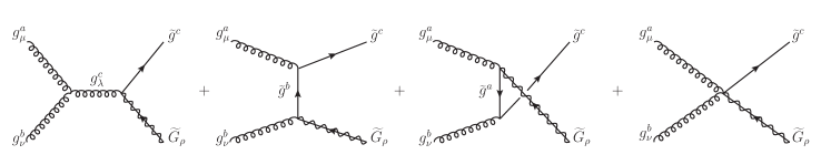
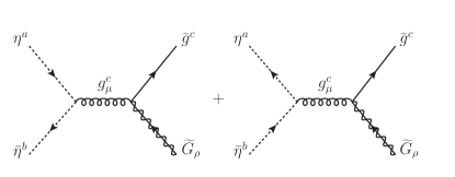
Figure 1: The relevant diagrams for the process $gg\to{\tilde{g}}{\widetilde{G}}$. In the top row are displayed in turn the $s$, $t$, $u$ channels and the quartic vertex $x$. In the bottom row the Faddeev–Popov ghosts diagrams are shown. Although here we present only the $SU(3)_{c}$ case, the same diagrams appear also for the $SU(2)_{L}$ gauge group, but not for the $U(1)_{Y}$.

As the gravitino is the superpartner of the graviton, its interactions are suppressed by the inverse of the reduced Planck mass $M_{\text{P}}=(8\pi\,G)^{-1/2}$. Hence, the dominant contributions to its production, in leading order of the gauge group couplings, are processes of the form $a\,b\rightarrow c\,\widetilde{G}$, where $\widetilde{G}$ stands for gravitino and $a$, $b$, $c$ can be three superpartners or one superpartner and two SM particles. The possible processes and the corresponding squared amplitudes in $SU(3)_{c}$ are given in Table 2, where for their denotation by the letters A-J we follow the “historical” notation of Ellis:1984eq .

Squared matrix elements for gravitino production in $SU(3)_{c}$ in terms of $g_{3}^{2}\,Y_{3}/M_{\text{P}}^{2}$ assuming massless particles, with $Y_{3}=1+m^{2}_{{\tilde{g}}}/(3m^{2}_{\tiny 3/2})$. The Casimir operators are $C_{3}=24$ and $C^{\prime}_{3}=48$. $X$ Process $|{\cal M}_{X,\rm full}|^{2}$ $|{\cal M}_{X,\rm sub}|^{2}$ A $gg\to{\tilde{g}}{\widetilde{G}}$ $4C_{3}(s+2t+2t^{2}/s)$ $-2sC_{3}$ B $g{\tilde{g}}\to g{\widetilde{G}}$ $-4C_{3}(t+2s+2s^{2}/t)$ $2tC_{3}$ C ${\tilde{q}}g\to q{\widetilde{G}}$ $2sC^{\prime}_{3}$ $0$ D $gq\to{\tilde{q}}{\widetilde{G}}$ $-2tC^{\prime}_{3}$ $0$ E ${\tilde{q}}q\to g{\widetilde{G}}$ $-2tC^{\prime}_{3}$ $0$ F ${\tilde{g}}{\tilde{g}}\to{\tilde{g}}{\widetilde{G}}$ $8C_{3}(s^{2}+t^{2}+u^{2})^{2}/(stu)$ $0$ G $q{\tilde{g}}\to q{\widetilde{G}}$ $-4C^{\prime}_{3}(s+s^{2}/t)$ $0$ H ${\tilde{q}}{\tilde{g}}\to{\tilde{q}}{\widetilde{G}}$ $-2C^{\prime}_{3}(t+2s+2s^{2}/t)$ $0$ I $q{\tilde{q}}\to{\tilde{g}}{\widetilde{G}}$ $-4C^{\prime}_{3}(t+t^{2}/s)$ $0$ J ${\tilde{q}}{\tilde{q}}\to{\tilde{g}}{\widetilde{G}}$ 2 $C^{\prime}_{3}(s+2t+2t^{2}/s)$ $0$

In $SU(3)_{c}$, the particles $a$, $b$, and $c$ could be gluons $g$, gluinos ${\tilde{g}}$, quarks $q$, or/and squarks ${\tilde{q}}$. Analogous processes happen in $SU(2)_{L}$ or $U(1)_{Y}$, where the gluino mass $m_{\tilde{g}}\equiv M_{3}$ becomes $M_{2}$ or $M_{1}$, respectively. In the factor $Y_{N}\equiv 1+{m_{\lambda_{N}}^{2}/(3m^{2}_{\tiny 3/2})}$, where $m_{\lambda_{N}}=\{M_{1},M_{2},M_{3}\}$ and $m_{\tiny 3/2}$ is the gravitino mass, the unity is related to the 3/2 gravitino components and the rest to the 1/2 goldstino part. As an example in Fig. 1 we present the relevant diagrams for the process A of table 2. For the calculation of the spin 3/2 part in the amplitudes, following Rychkov:2007uq , we have employed the gravitino polarization sum

$$\Pi^{\tiny 3/2}_{\mu\nu}(P)=\sum_{i=\pm 3/2}\Psi^{(i)}_{\mu}\,\overline{\Psi}^{(i)}_{\nu}=-\frac{1}{2}\gamma_{\mu}\mathchoice{\ooalign{$\hfil\displaystyle\mkern 0.0mu/\hfil$\crcr$\displaystyle P$}}{\ooalign{$\hfil\textstyle\mkern 0.0mu/\hfil$\crcr$\textstyle P$}}{\ooalign{$\hfil\scriptstyle\mkern 0.0mu/\hfil$\crcr$\scriptstyle P$}}{\ooalign{$\hfil\scriptscriptstyle\mkern 0.0mu/\hfil$\crcr$\scriptscriptstyle P$}}\gamma_{\nu}-\mathchoice{\ooalign{$\hfil\displaystyle\mkern 0.0mu/\hfil$\crcr$\displaystyle P$}}{\ooalign{$\hfil\textstyle\mkern 0.0mu/\hfil$\crcr$\textstyle P$}}{\ooalign{$\hfil\scriptstyle\mkern 0.0mu/\hfil$\crcr$\scriptstyle P$}}{\ooalign{$\hfil\scriptscriptstyle\mkern 0.0mu/\hfil$\crcr$\scriptscriptstyle P$}}g_{\mu\nu}\,,$$ (1)

where $\Psi_{\mu}$ is the gravitino spinor and $P$ its momentum. As in Rychkov:2007uq , for the goldstino spin 1/2 part the nonderivative approach is used Moroi:1995fs ; Pradler:2007ne . The result for the full squared amplitude has been proved to be the same, either in the derivative or the nonderivative approach Lee:1998aw .

The Casimir operators in Table 2 are $C_{N}=\sum_{a,b,c}|f^{abc}|^{2}=N(N^{2}-1)=\{0,6,24\}$ and $C_{N}^{\prime}=\sum^{\phi}_{a,i,j}|T^{a}_{ij}|^{2}=\{11,21,48\}$, where $\sum^{\phi}_{a,i,j}$ denotes the sum over all involved chiral multiplets and group indices. $f^{abc}$ and $T^{a}$ are the group structure constants and generators, respectively. Processes A, B and F are not present in $U(1)_{Y}$ because $C_{1}=0$. The masses for the particles $a$, $b$ and $c$ are assumed to be zero. In the third column of Table 2 we present for each process the square of the full amplitude, which is the sum of individual amplitudes,

$$|{\cal M}_{X,\rm full}|^{2}=|{\cal M}_{X,s}+{\cal M}_{X,t}+{\cal M}_{X,u}+{\cal M}_{X,x}|^{2}\,,$$ (2)

where the indices $s$, $t$, $u$ indicate the diagrams which are generated by the exchange of a particle in the corresponding channel and the index $x$ stands for the diagram involving a quartic vertex. The so-called $D-$graph, following the terminology of Rychkov:2007uq , is illustrated in Fig. 2 for the case of the gluino-gluon loop. Its contribution is the sum of the squared amplitudes for the $s$, $t$ and $u$ channel graphs,

$$|{\cal M}_{X,D}|^{2}=|{\cal M}_{X,s}|^{2}+|{\cal M}_{X,t}|^{2}+|{\cal M}_{X,u}|^{2}\,,$$ (3)

plus $1\to 2$ processes. This can be understood by applying the optical theorem. Hence, from the imaginary part of the loop graphs one computes the sum of the decays ($1\to 2$) and the scattering amplitudes ($2\to 2$). In our case, we use resummed thermal propagators for the gauge boson and gaugino and by applying cutting rules one sees that a $D-$graph describes both the scattering amplitudes appearing in (3) and decay amplitudes.

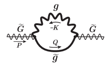
Figure 2: The one-loop thermally corrected gravitino self-energy ($D-$graph) for the case of $SU(3)_{c}$. The thick gluon and gluino lines denote resummed thermal propagators. The $SU(2)_{L}$ and $U(1)_{Y}$ cases have been also taken into account in our calculation.

The subtracted part of the squared amplitudes is the difference between the full amplitudes (2) and the amplitudes already included in the $D-$graph (3), i.e.

$$|{\cal M}_{X,\rm sub}|^{2}=|{\cal M}_{X,\rm full}|^{2}-|{\cal M}_{X,D}|^{2}\,.$$ (4)

For the processes B, F, G, and H, the corresponding amplitudes are IR divergent. For this reason we follow the more elegant method comprising the separation of the total scattering rate into two parts, the subtracted and the $D-$graph part. It is worth to mention that for the processes with incoming or/and outgoing gauge bosons, we have checked explicitly the gauge invariance for $|{\cal M}_{X,\rm full}|^{2}$. On the other hand, we note that $|{\cal M}_{X,\rm sub}|^{2}$ is gauge dependent. As it has been pointed out in Rychkov:2007uq the splitting of the amplitudes in resummed and non-resummed contributions violates the gauge invariance. Therefore a gauge dependence of the result is expected.

To sum up, the gravitino production rate $\gamma_{\tiny 3/2}$ consists of three parts: (i) the subtracted rate $\gamma_{\rm sub}$ (ii) the $D-$graph contribution $\gamma_{\rm D}$ and (iii) the top Yukawa rate $\gamma_{\rm top}$,

$$\gamma_{\tiny 3/2}=\gamma_{\rm sub}+\gamma_{\rm D}+\gamma_{\rm top}\,.$$ (5)

Below, these three contributions are discussed in detail.

2.1 The subtracted rate

In the fourth column of Table 2 we present the so-called subtracted part (4), which is the sum of the interference terms among the four types of diagrams ($s$, $t$, $u$, $x$), plus the $x$-diagram squared, for each process. The subtracted part is nonzero only for the processes A and B. Note that in Rychkov:2007uq the subtracted part for the processes H and J is also nonzero; we assume that the authors had used the squark-squark-gluino-goldstino Feynman rule as given in Bolz:2000xi , where a factor $\gamma_{5}$ is indeed missing. In contrast, we are using the correct Feynman rule as given in Pradler:2007ne .

To calculate the subtracted rate for the processes $a\,b\rightarrow c\,\widetilde{G}$, we use the general form

$$\gamma=\frac{1}{(2\pi)^{8}}\int \frac{{\rm d^{3}}\mathbf{p}_{a}}{2E_{a}}\,\frac{{\rm d^{3}}\mathbf{p}_{b}}{2E_{b}}\,\frac{{\rm d^{3}}\mathbf{p}_{c}}{2E_{c}}\,\frac{{\rm d^{3}}\mathbf{p}_{\widetilde{G}}}{2E_{\widetilde{G}}}\,\,|{\cal M}|^{2}\,f_{a}\,f_{b}\,(1\pm f_{c})\,\,\delta^{4}(P_{a}+P_{b}-P_{c}-P_{\widetilde{G}})\,,$$ (6)

where $f_{i}$ stands for the usual Bose and Fermi statistical densities

$$f_{B|F}={1\over e^{E\over T}\mp 1}\,.$$ (7)

In the temperature range of interest, all particles but the gravitino are in thermal equilibrium. For the gravitino the statistical factor $f_{\tiny{\widetilde{G}}}$ is negligible. Thus, $1-f_{\tiny{\widetilde{G}}}\simeq 1$, as it is already used in (6). Furthermore, backward reactions are neglected. In addition, the simplification $1\pm f_{c}\simeq 1$ is usually applied, making the analytic calculation of (6) possible. In our case there is no such reason. We keep the factor $1\pm f_{c}$ and consequently we proceed calculating the subtracted rate numerically. As it was argued in Bolz:2000xi and we have checked numerically the effect of taking into account the statistical factor $f_{c}$ can be around $-10$% ($+20$%) if $c$ is a fermion (boson).

The contribution of the processes A and B, for each gauge group, can be read from Table 2 as

$$|{\cal M}_{A,\rm sub}|^{2}+|{\cal M}_{B,\rm sub}|^{2}=\frac{g_{N}^{2}}{M_{\text{P}}^{2}}\left(1+\frac{m^{2}_{\lambda_{N}}}{3m^{2}_{\tiny 3/2}}\right)C_{N}(-s+2t)\,.$$ (8)

In (8), a factor $1/2$ is already included for the process A due to the two identical incoming particles. Substituting  (8) in  (6), the subtracted rate is obtained as

$$\gamma_{\mathrm{sub}}=\frac{T^{6}}{M_{\text{P}}^{2}}\sum_{N=1}^{3}g_{N}^{2}\left(1+\frac{m^{2}_{\lambda_{N}}}{3m^{2}_{\tiny 3/2}}\right)C_{N}\left(-{\cal C}_{\scriptscriptstyle\rm BBF}^{s}+2\,{\cal C}_{\scriptscriptstyle\rm BFB}^{t}\right)\,.$$ (9)

The numerical factors, calculated by using the Cuba library Hahn:2004fe , are ${\cal C}_{\scriptscriptstyle\rm BBF}^{s}=0.25957\times 10^{-3}$ and ${\cal C}_{\scriptscriptstyle\rm BFB}^{t}=-0.13286\times 10^{-3}\,.$ The subscripts B and F specify if the particles are bosons or fermions, respectively, and the superscripts determine if the squared amplitude is proportional to $s$ or $t$. It is easy to see that our result for the subtracted part unlike in Rychkov:2007uq is negative. This is not unphysical, since the total rate and not the subtracted one is bound to be positive.

2.2 The $D-$graph contribution

As it has been discussed above, Eq. (3) describes the relation between the $D-$graph and the sum of the squared amplitudes for the $s$, $t$, and $u$ channels. In the $D-$graph contribution, we will implement the resummed thermal corrections to the gauge boson and gaugino propagators. Like in Rychkov:2007uq using the gravitino polarization sum (1), we nullify the corresponding quark-squark $D-$graph. Although in Fig. 2 the gluino-gluon thermal loop is displayed, the contributions of all the gauge groups have been included in our analysis. The momentum flow used to calculate the $D-$graph can be depicted in Fig. 2. That is ${\widetilde{G}}(P)\to g(K)+{\tilde{g}}(Q)$, with $P=(p,p,0,0)\,,\,K=(k_{0},k\cos\theta_{k},k\sin\theta_{k},0)\,\,\text{and}\,\,Q=(q_{0},q\cos\theta_{q},q\sin\theta_{q},0)$, where $\theta_{k,q}$ are the polar angles of the corresponding 3-momenta $\mathbf{k},\mathbf{q}$ in spherical coordinates.

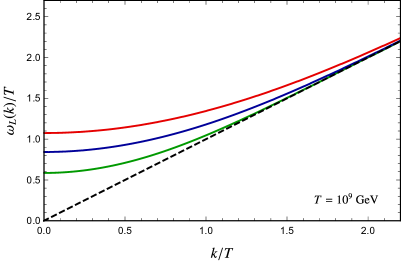
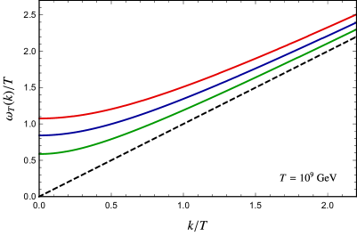
Figure 3: Dispersion relations for longitudinal (left) and transverse (right) vector bosons. The colored curves represent the $SU(3)_{c}$ (red), $SU(2)_{L}$ (blue), and $U(1)_{Y}$ (green) cases respectively. The dashed black line is the light-cone boundary. In both cases we have chosen $T=10^{9}\,\;\mathrm{GeV}$.

The non-time-ordered gravitino self-energy $\Pi^{<}(P)$ can be expressed in terms of the thermally resummed gaugino ${}^{*}S^{<}(Q)$ and gauge boson ${}^{*}D^{<}_{\mu\nu}(K)$ propagators as Bolz:2000fu ; Rychkov:2007uq

$$\Pi^{<}(P) = {1\over 16M^{2}_{P}}\sum_{N=1}^{3}n_{N}\left(1+{m^{2}_{\lambda_{N}}\over 3m^{2}_{\tiny 3/2}}\right)\int{{\rm d}^{4}K\over(2\pi)^{4}}\,{\rm Tr}\left[\mathchoice{\ooalign{$\hfil\displaystyle\mkern 0.0mu/\hfil$\crcr$\displaystyle P$}}{\ooalign{$\hfil\textstyle\mkern 0.0mu/\hfil$\crcr$\textstyle P$}}{\ooalign{$\hfil\scriptstyle\mkern 0.0mu/\hfil$\crcr$\scriptstyle P$}}{\ooalign{$\hfil\scriptscriptstyle\mkern 0.0mu/\hfil$\crcr$\scriptscriptstyle P$}}[\mathchoice{\ooalign{$\hfil\displaystyle\mkern 0.0mu/\hfil$\crcr$\displaystyle K$}}{\ooalign{$\hfil\textstyle\mkern 0.0mu/\hfil$\crcr$\textstyle K$}}{\ooalign{$\hfil\scriptstyle\mkern 0.0mu/\hfil$\crcr$\scriptstyle K$}}{\ooalign{$\hfil\scriptscriptstyle\mkern 0.0mu/\hfil$\crcr$\scriptscriptstyle K$}},\gamma^{\mu}]\,{}^{*}S^{<}(Q)[\mathchoice{\ooalign{$\hfil\displaystyle\mkern 0.0mu/\hfil$\crcr$\displaystyle K$}}{\ooalign{$\hfil\textstyle\mkern 0.0mu/\hfil$\crcr$\textstyle K$}}{\ooalign{$\hfil\scriptstyle\mkern 0.0mu/\hfil$\crcr$\scriptstyle K$}}{\ooalign{$\hfil\scriptscriptstyle\mkern 0.0mu/\hfil$\crcr$\scriptscriptstyle K$}},\gamma^{\nu}]\,{}^{*}D^{<}_{\mu\nu}(K)\right]\,,$$ (34)

where

$${}^{*}S^{<}(Q) = {f_{F}(q_{0})\over 2}\left[(\gamma_{0}-{\boldsymbol{\gamma}}\cdot\mathbf{q}/q)\,\rho_{+}(Q)+(\gamma_{0}+{\boldsymbol{\gamma}}\cdot\mathbf{q}/q)\,\rho_{-}(Q)\right]\,,$$ (35)

$${}^{*}D^{<}_{\mu\nu}(K) = f_{B}(k_{0})\left[\Pi_{\mu\nu}^{T}\,\rho_{T}(K)+\Pi_{\mu\nu}^{L}{k^{2}\over K^{2}}\,\rho_{L}(K)+\xi{K_{\mu}K_{\nu}\over K^{4}}\right]\,,$$

with $\xi$ being the gauge parameter, taken $\xi=1$ in our calculation and $n_{N}=\{1,3,8\}$. The spectral densities for longitudinal and transverse bosons are given by

$$\rho_{L}(K)=-2{\rm Im}\frac{K^{2}}{k^{2}}\frac{1}{K^{2}-\pi_{0}-\pi_{L}}\quad\quad\quad\text{and}\quad\quad\quad\rho_{T}(K)=-2{\rm Im}\frac{1}{K^{2}-\pi_{0}-\pi_{T}}\,,$$ (36)

while the fermionic ones are

$$\rho_{\pm}(Q)=-{\rm Im}\left\{\frac{q_{0}\mp q}{2}\left(1+\frac{1}{2\pi^{2}}\Big{[}{m_{F}^{2}\over T^{2}}\Big{(}2-\ln{-Q^{2}\over\mu^{2}}\Big{)}\Big{]}\right)+{m_{F}^{2}\over T^{2}}F_{\pm}\right\}^{-1}\,.$$ (37)

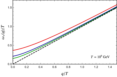
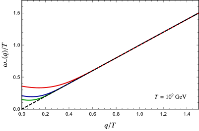
Figure 4: Dispersion relations for fermions (left) and fermion holes (right). The colored curves represent the $SU(3)_{c}$ (red), $SU(2)_{L}$ (blue), and $U(1)_{Y}$ (green) cases respectively. The dashed black line is the light-cone boundary. In both cases we have chosen $T=10^{9}\,\;\mathrm{GeV}$.

The longitudinal and the transverse projectors $\Pi_{\mu\nu}^{L}$, $\Pi_{\mu\nu}^{T}$, as well as the functions $\pi_{L}$, $\pi_{T}$, $\pi_{0}$, $F_{\pm}$ and the thermal mass $m_{F}$ can be found in Appendices B and C of Rychkov:2007uq . The spectral densities (36),(37) contain Landau damping contributions stemming from the imaginary part of the self-energies below and above the light-cone and also quasi-particles contributions for $k_{0}^{2}>k^{2}$ (and $q_{0}^{2}>q^{2}$). The quasi-particles contributions have the form $\delta(k_{0}\pm\omega_{L,T})$ for the bosons and $\delta(q_{0}\pm\omega_{\pm})$ for the fermions, and are multiplied by suitable residues (see Bellac:2011kqa for the analytical expressions of the residues in the HTL approximation). The positions of the poles $\omega_{L,T}$ and $\omega_{\pm}$ can be very well approximated using the HTL limit, as it is discussed in Rychkov:2007uq ; Peshier:1998dy . This argument is indeed true as we have seen numerically, but in order to be completely accurate, in Figs. 3 and 4 we display the dispersion relations for bosons and fermions, for the three gauge groups, beyond the HTL approximation.

To compute the production rate related to the $D-$graph $\gamma_{D}$, we will use its definition Bellac:2011kqa

$$\gamma_{D}=\int{{\rm d^{3}\mathbf{p}}\over 2p_{0}(2\pi)^{3}}\,\,\Pi^{<}(p)\,$$ (38)

and after appropriate manipulations , we obtain

$$\gamma_{\rm D} = {1\over 4(2\pi)^{5}M_{\text{P}}^{2}}\sum_{N=1}^{3}n_{N}\left(1+{m^{2}_{\lambda_{N}}\over 3m^{2}_{\tiny 3/2}}\right)\int_{0}^{\infty}{\rm d}p\int_{-\infty}^{\infty}{\rm d}k_{0}\int_{0}^{\infty}{\rm d}k\int_{|k-p|}^{k+p}{\rm d}q\,\,k\,f_{B}(k_{0})\,f_{F}(q_{0})$$

$$\times\Big{[}\rho_{L}(K)\,\rho_{-}(Q)\,(p-q)^{2}\big{(}(p+q)^{2}-k^{2}\big{)}+\rho_{L}(K)\,\rho_{+}(Q)\,(p+q)^{2}\big{(}k^{2}-(p-q)^{2}\big{)}$$

$$+\,\,\rho_{T}(K)\,\rho_{-}(Q)\,\big{(}k^{2}-(p-q)^{2}\big{)}\Big{(}(1+k_{0}^{2}/k^{2}\big{)}\big{(}k^{2}+(p+q)^{2}\big{)}-4k_{0}(p+q)\Big{)}$$

$$+\,\,\rho_{T}(K)\,\rho_{+}(Q)\,\big{(}(p+q)^{2}-k^{2}\big{)}\Big{(}(1+k_{0}^{2}/k^{2})\big{(}k^{2}+(p-q)^{2}\big{)}-4k_{0}(p-q)\Big{)}\Big{]}\,,$$

where $q_{0}=p-k_{0}\,.$ The spectral functions $\rho_{L,T}$ and $\rho_{\pm}$ can be found in Eq. (3.7) in Rychkov:2007uq . The thermally corrected one-loop self-energy for gauge bosons, scalars and fermions that we have used in calculating these spectral functions can be found in Weldon:1982aq ; Weldon:1982bn ; Weldon:1989ys ; Weldon:1996kb ; Peshier:1998dy ; Weldon:1999th . Comparing (2.2) with the corresponding analytical result given in Eqs. (4.6) and (4.7) in Rychkov:2007uq , one can notice that they differ on the overall factor and on the number of independent phase-space integrations. Our analytical result has been checked using various frames for the momenta flow into the loop.

2.3 The top Yukawa rate

The production rate resulting from the top-quark Yukawa coupling $\lambda_{t}$ is given by Rychkov:2007uq

$$\gamma_{\mathrm{top}}=\frac{T^{6}}{M_{\text{P}}^{2}}\,72\,\,{\cal C}_{\scriptscriptstyle\rm BBF}^{s}\,\lambda_{t}^{2}\left(1+\frac{A_{t}^{2}}{3m^{2}_{\tiny 3/2}}\right)\,,$$ (40)

where $A_{t}$ is the trilinear stop supersymmetry breaking soft parameter and ${\cal C}_{\scriptscriptstyle\rm BBF}^{s}=0.25957\times 10^{-3}$. Since this contribution stems from the process squark-squark $\rightarrow$ Higgsino-gravitino, only the numerical factor ${\cal C}_{\rm BBF}^{s}$ is involved.

The values of the constants $c_{N}$ and $k_{N}$ that parametrize our result (17). Each line corresponds in turn to the particular gauge group, $U(1)_{Y}$, $SU(2)_{L}$ or $SU(3)_{c}$.   Gauge group  $c_{N}$     $k_{N}$  $U(1)_{Y}$  41.937     0.824  $SU(2)_{L}$  68.228     1.008  $SU(3)_{c}$  21.067     6.878

3 Parameterizing the result

Following Ellis:2015jpg we parametrize the results (9) and (2.2) using the gauge couplings $g_{1},g_{2}$ and $g_{3}\,.$ Thus

$$\gamma_{\mathrm{sub}}+\gamma_{\mathrm{D}}={3\zeta(3)\over 16\pi^{3}}\,\frac{T^{6}}{M_{\text{P}}^{2}}\sum_{N=1}^{3}c_{N}\,g_{N}^{2}\left(1+{m^{2}_{\lambda_{N}}\over 3m^{2}_{\tiny 3/2}}\right)\ln\left({k_{N}\over g_{N}}\right),$$ (17)

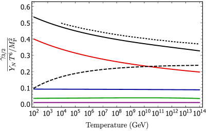
Figure 5: The gravitino production rates in units of $Y_{N}\,T^{6}/M_{\text{P}}^{2}$. The solid curves represent in order the total rate (black) given by (5), the $SU(3)_{c}$ (red), $SU(2)_{L}$ (blue), and $U(1)_{Y}$ (green) rates given by (17), and the top Yukawa rate (purple) given by (40). The upper short dashed curve is the total production rate obtained in Rychkov:2007uq , while the lower long dashed curve obtained in Pradler:2006hh . The top Yukawa coupling $\lambda_{t}$ has been taken equal to 0.7 and the trilinear coupling $A_{t}$ has been ignored so that our result can be directly compared with that in Rychkov:2007uq .

where the constants $c_{N}$ and $k_{N}$ depend on the gauge group and their values are given in Table 2.3. In Fig. 5 we summarize our numerical results for the gravitino production rates divided by $Y_{N}\,T^{6}/M_{\text{P}}^{2}$. Especially, for the case of the top Yukawa contribution, in $Y_{N}$ the $m^{2}_{\lambda_{N}}$ has to be replaced by $A_{t}^{2}$. The colored solid curves represent the $SU(3)_{c}$ (red), $SU(2)_{L}$ (blue), and $U(1)_{Y}$ (green) rates given by (17) and the top Yukawa rate (purple) given by (40), while the black solid curve is the total result given by (5). The dashed black curve corresponds to the total result from Rychkov:2007uq . For an easy comparison, we have chosen $\lambda_{t}=0.7$. The framework of our calculation is the Minimal Supersymmetric Standard Model (MSSM) gauge group structure $SU(3)_{c}\times SU(2)_{L}\times U(1)_{Y}$. It is interesting that our result for the total gravitino production rate is only $5\%-11\%$ smaller than that in Rychkov:2007uq . We are not able to provide a detailed quantitative explanation.

For convenience, in Fig. 5, universal gauge coupling unification is assumed at the Grand Unification (GUT) scale $\simeq 2\times 10^{16}\,\;\mathrm{GeV}$, but the result in (17) can be used in a more general framework. Equation (17) along with the numbers in Table 2.3 are the main results of this talk.

4 Thermal Abundance of Gravitino

The relevant Boltzmann equation for the gravitino number density $n_{\tiny 3/2}$ can be written as

$$\frac{d{n}_{\tiny 3/2}}{dt}+3Hn_{\tiny 3/2}=\gamma_{\tiny 3/2}\,,$$ (18)

where $H$ is the expansion rate of the Universe. The gravitino abundance $Y_{\tiny 3/2}$ is defined as the ratio of $n_{\tiny 3/2}$ to the number density of any single bosonic degree of freedom (DOF), $n_{\rm rad}=\zeta(3)T^{3}/\pi^{2}$. That is

$$Y_{\tiny 3/2}={n_{\tiny 3/2}\over n_{\rm rad}}\,,$$ (19)

From (18) and (19) we obtain that the gravitino abundance for temperatures much lower than the reheating temperature, i.e. $T\ll T_{\rm reh}$ is given by Ellis:2015jpg

$$Y_{\tiny 3/2}(T)\simeq{\gamma_{\tiny 3/2}(T_{\rm reh})\over H(T_{\rm reh})\,\,n_{\rm rad}(T_{\rm reh})}\,\,{g_{*s}(T)\over g_{*s}(T_{\rm reh})}\,,$$ (20)

where $g_{*s}$ are the entropy density DOFs in the MSSM. Notice that Eq. (20) is consistent with the assumption that the inflaton decays are instantaneous, as the Universe is thermalizing. The case of not instantaneous inflaton decay has been also studied in Ellis:2015jpg ; Garcia:2017tuj .

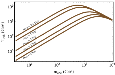
Figure 6: The thick show the $3\sigma$ regions where $\Omega_{\mathrm{DM}}$ is equal to the gravitino abundance for various values of $m_{\tiny 1/2}$. As previously the top Yukawa coupling is $\lambda_{t}=0.7$ and the trilinear coupling $A_{t}$ has been ignored.

According to the latest data from the Planck satellite Aghanim:2018eyx , the cosmological accepted value for the DM density in the Universe is $\Omega_{\mathrm{DM}}h^{2}=0.1198\pm 0.0012$. Assuming that the entire thermal gravitino abundance is the observed DM, we obtain that

$$\Omega_{\mathrm{DM}}h^{2}={\rho_{\tiny 3/2}(t_{0})\,h^{2}\over\rho_{\rm cr}}\simeq 1.33\times 10^{24}\,{m_{\tiny 3/2}\,\,\gamma_{\tiny 3/2}(T_{\rm reh})\over T_{\rm reh}^{5}}\,,$$ (21)

where $\rho_{\tiny 3/2}$ is the gravitino mass density, $\rho_{\rm cr}=3\,H_{0}^{2}M_{\text{P}}^{2}$ is the critical energy density, $H_{0}=100\,h\,{\rm km/(s\,Mpc)}$ is the Hubble constant today, and $T_{0}=2.725\,K$ the temperature of the cosmic microwave background in the current epoch. Assuming the MSSM content, the entropy DOFs at the relevant temperatures are $g_{*s}(T_{0})=43/11$ and $g_{*s}(T_{\rm reh})=915/4$. Figure 6 illustrates the $3\sigma$ regions resulting from (21) for various values of $m_{\tiny 1/2}$ between $750\;\mathrm{GeV}$ and $4\;\mathrm{TeV}$. In this, the top Yukawa coupling has been choosen to have the value $\lambda_{t}=0.7$ as previously, and the trilinear coupling $A_{t}$ has been ignored. As before, a gauge coupling unification and a universal gaugino mass $m_{\tiny 1/2}$ are assumed at the GUT scale $\simeq 2\times 10^{16}\,\;\mathrm{GeV}$.

In the large gravitino mass limit, $m_{\tiny 1/2}\ll m_{\tiny 3/2}$, the characteristic factor $m_{\lambda_{N}}^{2}/(3m^{2}_{\tiny 3/2})$ becomes negligible and so the reheating temperature is $m_{\tiny 1/2}$ independent as it is shown in Fig. 6. The recent LHC data on gluino searches Aaboud:2017hrg ; Sirunyan:2019ctn , suggest that $m_{\tiny 1/2}\gtrsim\textit{}750\,\;\mathrm{GeV}$, and thus according to Fig. 6 the maximum reheating temperature $T_{\mathrm{reh}}\simeq 10^{9}\,\;\mathrm{GeV}$ corresponds to a gravitino mass $m_{\tiny 3/2}\simeq 550\,\;\mathrm{GeV}$. For the same gravitino mass, $m_{\tiny 1/2}$ can go up to $3-4\;\mathrm{TeV}$, for a reheating temperature an order of magnitude smaller $T_{\mathrm{reh}}\simeq 10^{8}\;\mathrm{GeV}$.

5 Conclusions

In this talk, we have presented a calculation of the gravitino thermal abundance, using the full one-loop thermally corrected gravitino self-energy Eberl:2020fml . Having amended the main analytical formulas for the gravitino production rate, we have computed it numerically without any approximation. In addition we provide a simple and useful parametrization of our final result. Moreover, in the context of minimal supergravity models, assuming gaugino mass unification, we have updated the bounds on the reheating temperature for certain gravitino masses. In particular, saturating the current LHC gluino mass limit $m_{\tilde{g}}\gtrsim 2100\;\mathrm{GeV}$, we find that a maximum reheating temperature $T_{\mathrm{reh}}\simeq 10^{9}\;\mathrm{GeV}$ is compatible to a gravitino mass $m_{\tiny 3/2}\simeq 500-600\,\;\mathrm{GeV}$.

As for the constraints on the reheating temperature, we have applied the cosmological data on gravitino DM scenarios. This tells us whether thermal leptogenesis is a possible mechanism for generating baryon asymmetry of the Universe. Successful thermal leptogenesis requires high temperature, $T_{\mathrm{reh}}\gtrsim 2\times 10^{9}\,\;\mathrm{GeV}$ Giudice:2003jh ; Antusch:2006gy ; Buchmuller:2005eh , which is marginally bigger than the maximum reheating temperature obtained in our model using the lowest $m_{\tiny 1/2}$ mass demonstrated in the recent LHC data Aaboud:2017hrg ; Sirunyan:2019ctn . In any case, there are many alternative models for baryogenesis. In addition, as it has been pointed out before, the thermal gravitino abundance is in general a part of the whole DM density and the inclusion of other components will affect the phenomenological analysis.

References

- (1) H. Eberl, I. D. Gialamas and V. C. Spanos, “Gravitino thermal production revisited”, Phys. Rev. D 103, no.7, 075025 (2021), arXiv:2010.14621 [hep-ph].
- (2) R. Kallosh, L. Kofman, A. D. Linde and A. Van Proeyen, “Gravitino production after inflation”, Phys. Rev. D 61, 103503 (2000), arXiv:hep-th/9907124.
- (3) G. F. Giudice, A. Riotto and I. Tkachev, “Thermal and nonthermal production of gravitinos in the early universe”, JHEP 11, 036 (1999), arXiv:hep-ph/9911302.
- (4) H. P. Nilles, M. Peloso and L. Sorbo, “Nonthermal production of gravitinos and inflatinos”, Phys. Rev. Lett. 87, 051302 (2001), arXiv:hep-ph/0102264.
- (5) M. Kawasaki, F. Takahashi and T. T. Yanagida, “Gravitino overproduction in inflaton decay”, Phys. Lett. B 638, 8-12 (2006), arXiv:hep-ph/0603265.
- (6) M. Endo, M. Kawasaki, F. Takahashi and T. T. Yanagida, “Inflaton decay through supergravity effects”, Phys. Lett. B 642, 518-524 (2006), arXiv:hep-ph/0607170.
- (7) J. Ellis, M. A. G. Garcia, D. V. Nanopoulos, K. A. Olive and M. Peloso, “Post-Inflationary Gravitino Production Revisited”, JCAP 03, 008 (2016), arXiv:1512.05701 [astro-ph.CO].
- (8) E. Dudas, Y. Mambrini and K. Olive, “Case for an EeV Gravitino”, Phys. Rev. Lett. 119, no.5, 051801 (2017), arXiv:1704.03008 [hep-ph].
- (9) K. Kaneta, Y. Mambrini and K. A. Olive, “Radiative production of nonthermal dark matter”, Phys. Rev. D 99, no.6, 063508 (2019), arXiv:1901.04449 [hep-ph].
- (10) M. A. G. Garcia, K. Kaneta, Y. Mambrini and K. A. Olive, “Inflaton Oscillations and Post-Inflationary Reheating”, JCAP 04, 012 (2021), arXiv:2012.10756 [hep-ph].
- (11) M. Kawasaki, K. Kohri, T. Moroi and A. Yotsuyanagi, “Big-Bang Nucleosynthesis and Gravitino”, Phys. Rev. D 78, 065011 (2008), arXiv:0804.3745 [hep-ph].
- (12) M. Kawasaki, K. Kohri, T. Moroi and Y. Takaesu, “Revisiting Big-Bang Nucleosynthesis Constraints on Long-Lived Decaying Particles”, Phys. Rev. D 97, no.2, 023502 (2018), arXiv:1709.01211 [hep-ph].
- (13) R. H. Cyburt, J. R. Ellis, B. D. Fields, K. A. Olive and V. C. Spanos, “Bound-State Effects on Light-Element Abundances in Gravitino Dark Matter Scenarios”, JCAP 11, 014 (2006), arXiv:astro-ph/0608562.
- (14) R. H. Cyburt, J. Ellis, B. D. Fields, F. Luo, K. A. Olive and V. C. Spanos, “Metastable Charged Sparticles and the Cosmological Li7 Problem”, JCAP 12, 037 (2012), arXiv:1209.1347 [astro-ph.CO].
- (15) S. Weinberg, “Cosmological Constraints on the Scale of Supersymmetry Breaking”, Phys. Rev. Lett. 48, 1303 (1982).
- (16) J. R. Ellis, J. E. Kim and D. V. Nanopoulos, “Cosmological Gravitino Regeneration and Decay”, Phys. Lett. B 145, 181-186 (1984).
- (17) M. Y. Khlopov and A. D. Linde, “Is It Easy to Save the Gravitino?”, Phys. Lett. B 138, 265-268 (1984).
- (18) T. Moroi, H. Murayama and M. Yamaguchi, “Cosmological constraints on the light stable gravitino”, Phys. Lett. B 303, 289-294 (1993).
- (19) M. Kawasaki and T. Moroi, “Gravitino production in the inflationary universe and the effects on big bang nucleosynthesis”, Prog. Theor. Phys. 93, 879-900 (1995), arXiv:hep-ph/9403364.
- (20) T. Moroi, “Effects of the gravitino on the inflationary universe”, PhD thesis, Tohoku U., 1995, arXiv:hep-ph/9503210 .
- (21) J. R. Ellis, D. V. Nanopoulos, K. A. Olive and S. J. Rey, “On the thermal regeneration rate for light gravitinos in the early universe”, Astropart. Phys. 4, 371-386 (1996), arXiv:hep-ph/9505438.
- (22) M. Bolz, W. Buchmuller and M. Plumacher, “Baryon asymmetry and dark matter”, Phys. Lett. B 443, 209-213 (1998), arXiv:hep-ph/9809381.
- (23) M. Bolz, A. Brandenburg and W. Buchmuller, “Thermal production of gravitinos”, Nucl. Phys. B 606, 518-544 (2001), [erratum: Nucl. Phys. B 790, 336-337 (2008)]
- (24) M. Bolz, “Thermal Production of Gravitinos”, PhD thesis, Hamburg U., 2000.
- (25) F. D. Steffen, “Gravitino dark matter and cosmological constraints”, JCAP 09, 001 (2006), arXiv:hep-ph/0605306.
- (26) J. Pradler and F. D. Steffen, “Thermal gravitino production and collider tests of leptogenesis”, Phys. Rev. D 75, 023509 (2007), arXiv:hep-ph/0608344.
- (27) J. Pradler and F. D. Steffen, “Constraints on the Reheating Temperature in Gravitino Dark Matter Scenarios”, Phys. Lett. B 648, 224-235 (2007), arXiv:hep-ph/0612291.
- (28) V. S. Rychkov and A. Strumia, “Thermal production of gravitinos”, Phys. Rev. D 75, 075011 (2007), arXiv:hep-ph/0701104.
- (29) J. Pradler, “Electroweak Contributions to Thermal Gravitino Production”, Diploma thesis, U. Vienna, 2006, arXiv:0708.2786 [hep-ph].
- (30) G. F. Giudice and R. Rattazzi, “Theories with gauge mediated supersymmetry breaking”, Phys. Rept. 322 (1999), 419-499, arXiv:hep-ph/9801271.
- (31) K. Choi, K. Hwang, H. B. Kim and T. Lee, “Cosmological gravitino production in gauge mediated supersymmetry breaking models”, Phys. Lett. B 467, 211-217 (1999), arXiv:hep-ph/9902291.
- (32) T. Asaka, K. Hamaguchi and K. Suzuki, “Cosmological gravitino problem in gauge mediated supersymmetry breaking models”, Phys. Lett. B 490, 136-146 (2000), arXiv:hep-ph/0005136.
- (33) K. Jedamzik, M. Lemoine and G. Moultaka, “Gravitino dark matter in gauge mediated supersymmetry breaking”, Phys. Rev. D 73, 043514 (2006), arXiv:hep-ph/0506129 .
- (34) E. W. Kolb, A. J. Long and E. Mcdonough, “Catastrophic Production of Slow Gravitinos”, [arXiv:2102.10113 [hep-th]].
- (35) E. W. Kolb, A. J. Long and E. Mcdonough, “The Gravitino Swampland Conjecture”, [arXiv:2103.10437 [hep-th]].
- (36) E. Dudas, M. A. G. Garcia, Y. Mambrini, K. A. Olive, M. Peloso and S. Verner, “Slow and Safe Gravitinos”, [arXiv:2104.03749 [hep-th]].
- (37) T. Terada, “Minimal Supergravity Inflation without Slow Gravitino”, [arXiv:2104.05731 [hep-th]].
- (38) N. Cribiori, D. Lüst and M. Scalisi, “The Gravitino and the Swampland”, [arXiv:2104.08288 [hep-th]].
- (39) A. Castellano, A. Font, A. Herráez and L. E. Ibáñez, “A Gravitino Distance Conjecture”, [arXiv:2104.10181 [hep-th]].
- (40) E. Braaten and R. D. Pisarski, “Soft Amplitudes in Hot Gauge Theories: A General Analysis”, Nucl. Phys. B 337, 569-634 (1990).
- (41) E. Braaten and T. C. Yuan, “Calculation of screening in a hot plasma”, Phys. Rev. Lett. 66, 2183-2186 (1991).
- (42) T. Lee and G. H. Wu, “Interactions of a single goldstino”, Phys. Lett. B 447, 83-88 (1999), arXiv:hep-ph/9805512.
- (43) T. Hahn, “CUBA: A Library for multidimensional numerical integration”, Comput. Phys. Commun. 168, 78-95 (2005), arXiv:hep-ph/0404043.
- (44) M. L. Bellac, “Thermal Field Theory”, Cambridge Monographs on Mathematical Physics, Cambridge.
- (45) H. Eberl, I. D. Gialamas and V. C. Spanos, In preparation.
- (46) H. A. Weldon, “Covariant Calculations at Finite Temperature: The Relativistic Plasma”, Phys. Rev. D 26, 1394 (1982).
- (47) H. A. Weldon, “Effective Fermion Masses of Order in High Temperature Gauge Theories with Exact Chiral Invariance”, Phys. Rev. D 26, 2789 (1982).
- (48) H. A. Weldon, “Dynamical Holes in the Quark–Gluon Plasma”, Phys. Rev. D 40, 2410 (1989).
- (49) H. A. Weldon, “Structure of the gluon propagator at finite temperature”, Annals Phys. 271, 141-156 (1999), arXiv:hep-ph/9701279.
- (50) A. Peshier, K. Schertler and M. H. Thoma, “One loop selfenergies at finite temperature”, Annals Phys. 266, 162-177 (1998), arXiv:hep-ph/9708434.
- (51) H. A. Weldon, “Structure of the quark propagator at high temperature”, Phys. Rev. D 61, 036003 (2000), arXiv:hep-ph/9908204.
- (52) J. Ellis, M. A. G. Garcia, N. Nagata, D. V. Nanopoulos and K. A. Olive, “Superstring-Inspired Particle Cosmology: Inflation, Neutrino Masses, Leptogenesis, Dark Matter & the SUSY Scale,” JCAP 01, 035 (2020), arXiv:1910.11755 [hep-ph].
- (53) M. A. G. Garcia, Y. Mambrini, K. A. Olive and M. Peloso, “Enhancement of the Dark Matter Abundance Before Reheating: Applications to Gravitino Dark Matter”, Phys. Rev. D 96, no.10, 103510 (2017), arXiv:1709.01549 [hep-ph].
- (54) N. Aghanim et al. [Planck], “Planck 2018 results. VI. Cosmological parameters”, Astron. Astrophys. 641, A6 (2020), arXiv:1807.06209 [astro-ph.CO].
- (55) M. Aaboud et al. [ATLAS], “Search for supersymmetry in final states with missing transverse momentum and multiple -jets in proton-proton collisions at TeV with the ATLAS detector”, JHEP 06, 107 (2018), arXiv:1711.01901 [hep-ex].
- (56) A. M. Sirunyan et al. [CMS], “Search for supersymmetry in proton-proton collisions at 13 TeV in final states with jets and missing transverse momentum”, JHEP 10, 244 (2019), arXiv:1908.04722 [hep-ex].
- (57) G. F. Giudice, A. Notari, M. Raidal, A. Riotto and A. Strumia, “Towards a complete theory of thermal leptogenesis in the SM and MSSM”, Nucl. Phys. B 685, 89-149 (2004), arXiv:hep-ph/0310123.
- (58) W. Buchmuller, R. D. Peccei and T. Yanagida, “Leptogenesis as the origin of matter”, Ann. Rev. Nucl. Part. Sci. 55, 311-355 (2005), arXiv:hep-ph/0502169 .
- (59) S. Antusch and A. M. Teixeira, “Towards constraints on the SUSY seesaw from flavour-dependent leptogenesis”, JCAP 02, 024 (2007), arXiv:hep-ph/0611232.