Electric and Magnetic Responses of Two-dimensional Dirac Electrons in Organic Conductor $\alpha$-(BETS)₂I₃

Abstract

Effect of spin-orbit coupling (SOC) on Dirac electrons in the organic conductor $\alpha$-(BETS)₂I₃ [BETS = bis(ethylenedithio)tetraselenafulvalene] has been examined by calculating electric conductivity and spin magnetic susceptibility. A tight-binding (TB) model with real and imaginary transfer energies is derived using first-principles density-functional theory method. The conductivity without the SOC depends on both anisotropies of the velocity of the Dirac cone and the tiling of the cone. Such conductivity is suppressed by the SOC, which gives rise to the imaginary part of the transfer energy. Due to the SOC, we find at low temperatures that the reduction of the conductivity becomes large and that the anisotropy of the conductivity is reduced. A nearly constant conductivity at high temperatures is obtained by an electron–phonon (e–p) scattering. Further, the property of the Dirac cone is examined for the spin susceptibility, which is mainly determined by the density of states (DOS). The result is compared with the case of the organic conductor $\alpha$-(BEDT-TTF)₂I₃ [BEDT-TTF=bis(ethylenedithio)tetrathiafulvalene], which provides the Dirac cone without the SOC. The relevance to experiments is discussed.

1 Introduction

Since the discovery in the graphene[1], massless Dirac fermion has been studied extensively. Especially the Dirac electron in an organic conductor, $\alpha$-(BEDT-TTF)₂I₃ [BEDT-TTF=bis(ethylenedithio)tetrathiafulvalene], was found as a bulk system.[2, 3, 4] The two-dimensional Dirac cone provides the density of states (DOS) vanishing linearly at the Fermi energy and a zero-gap state (ZGS). The energy band was calculated using a tight-binding (TB) model, where transfer energies are estimated from the extended Hückel method.[5] Such a Dirac cone was verified by a first-principles density functional theory (DFT) calculation.[6]

The ZGS has been studied in some organic conductors with isostructural salts, $\alpha$-D₂I₃ (D = ET, STF, and BETS), where ET = BEDT-TTF, STF = bis(ethylenedithio)diselenadithiafuluvalene), and BETS = bis(ethylenedithio)tetraselenafulvalene. These salts display an energy band with a Dirac cone, [3, 7, 8, 9] and the resistivity at high temperatures shows a nearly constant behavior. [10, 11, 12, 13, 14, 15] Such a constant resistivity behavior at high temperatures suggests a common feature of Dirac electrons in organic conductors. In contrast, the resistivity at low temperatures shows a different behavior depending on the salts. For $\alpha$-(ET)₂I₃, the insulating state is obtained by the charge ordering (CO), where A and A’ molecules in the unit cell become inequivalent due to breaking the inversion symmetry. [16, 17, 18] Under high pressures, the CO is absent. The resistivity shows only a slight enhancement with a minimum,[14] and the equivalence of A and A’ due to the inversion symmetry is shown from the spin susceptibility.[19, 20, 21] For $\alpha$-(BETS)₂I₃, the CO is absent, and the resistivity shows an enhancement but not an insulating state at ambient pressure, and an almost constant behavior under pressure.

The physical properties of Dirac electrons have been studied in terms of an effective Hamiltonian of the two-band model. [22, 23, 24] The conductivity with zero doping has been studied theoretically using a two-band model with a simple Dirac cone. The static conductivity at absolute zero temperature remains finite with a universal value, i.e., independent of the magnitude of impurity scattering owing to a quantum effect.[25] The effect of Dirac cone tilting shows the anisotropic conductivity and the deviation of the current from an applied electric field. [26] At finite temperatures, on the other hand, the conductivity depends on the magnitude of the impurity scattering, $\Gamma$, which is proportional to the inverse of the life time by the disorder. With increasing $T$, the conductivity remains unchanged for $T\ll\Gamma$, whereas it increases for $\Gamma\ll T$.[27] Noting that $\Gamma\sim$ 0.0003 eV for organic conductors,[4] a monotonic increase in the conductivity at finite temperature $T>0.0005$ eV is expected. However, the measured conductivity (or resistivity) of the above organic conductor shows an almost constant behavior at high temperatures. To comprehend such an exotic phenomenon, the acoustic phonon scatterings have been proposed as a possible mechanism, which was studied using a simple two-band model of the Dirac cone without tilting.  [28] Such a mechanism reasonably explains the conductivity in $\alpha$-(ET)₂I₃, described by the TB model.  [29] However, electric conductivity for $\alpha$-(BETS)₂I₃ has yet to be clarified theoretically.

The selenium-substituted analog $\alpha$-(BETS)₂I₃ has recently attracted attention as a possible Dirac electron at ambient pressure. The temperature crossover from the metal to insulating behavior around 50 K ($T_{MI}$) is lower than the CO transition temperature in $\alpha$-(ET)₂I₃.[10] To understand the origin of the increased resistivity at low temperatures, several groups studied whether the presence or absence of the CO transition at ambient pressure. At high temperatures, the spin susceptibility is similar between $\alpha$-(ET)₂I₃ and $\alpha$-(BETS)₂I₃.[30] However, the NMR suggests the inversion symmetry, which would indicate the absence of the CO in $\alpha$-(BETS)₂I₃.[31] Structural analysis based on x-ray diffraction also suggests no breaking the inversion symmetry around the $T_{MI}$ [32].

First-principles calculation for the low-temperature structure reveals a pair of anisotropic Dirac cones at a general $\bm{k}$-point, when the spin-orbit coupling (SOC) effect is ignored [32]. The Dirac cone band structure is robust, which is different from a previous DFT band structure for the 0.7 GPa structure, where Dirac point and electron-hole pockets coexist [33].

In contrast, when we consider the SOC effect, an indirect gap of $\sim$2 meV is opened at the Dirac points. The band gap size is generally consistent with the $T_{MI}$, since (semi) local density approximation in DFT slightly underestimates the experimental energy gap. The calculated $\mathbb{Z}_{2}$ topological invariant suggests the system is a weak topological insulator [32]. Shubnikov-de Haas oscillation measurement verified the absence of massless Dirac electrons at ambient pressure and low temperature, and the Dirac fermion phase appears under pressure [34]. Since the width of linear band dispersion is wider than the band gap, this system can exhibit the behavior of a Dirac electron at finite temperature. Moreover, it is not clear how the velocity anisotropy of the Dirac cone affects the electrical conductivity.

To derive a TB model from DFT band dispersions is crucial to comprehend the Dirac electrons properly.[35] However, efficient methods for extracting effective TB models, including the SOC, have not been fully established for molecular solids.[36, 37] In our previous work, it is found that the delocalized character of Se $p$ orbitals constrains the eigenvalues close to the Dirac points in a quite-narrow energy window, compared with the electronic state of $\alpha$-(ET)₂I₃ [38]. Therefore, the result of fitting to the DFT bands indicates that the number of relevant transfer integrals is significant. [38] To develop a reliable low-energy model Hamiltonian with a moderate number of transfer energies, we introduce site-potentials, which reasonably reproduce the spectrum of the DFT eigenvalues at several time-reversal invariant momenta (TRIM), and propose a precise TB model for the insulating state in $\alpha$-(BETS)₂I₃.

In this paper, we study the effect of the SOC on the anisotropic conductivity using the TB model of $\alpha$-(BETS)₂I₃,[38] which contains both real and imaginary parts in the transfer energy. By using such a TB model, we clarify the origin of the insulating behavior at low temperatures. It is also shown that the presence of acoustic phonons gives rise to the conductivity being nearly constant at high temperatures. The paper is organized as follows. In Sect. 2, the model and formulation are given for $\alpha$-(BETS)₂I₃. In Sect. 3, after examining the chemical potential and density of states (DOS), the conductivity and spin susceptibility are calculated, and the characteristics are demonstrated by comparing with those of $\alpha$-(ET)₂I₃.  [29] Section 4 is devoted to a summary and discussion of the relevance to experiments.

2 Model and Formulation

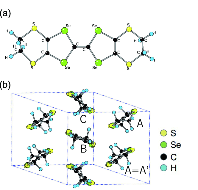
Figure 1: (Color online) (a) Molecular structure of BETS (= bis(ethylenedithio)tetraselenafulvalene), which has a glide symmetry to the center of the C=C bond. (b) Crystal structure of $\alpha$-(BETS)₂I₃ with four molecules of A, A’, B, and C in the unit cell forming a square lattice. The inversion center exists at the middle of A and A’, which are equivalent molecules. Transfer energies taken for nearest neighbor (NN) and next-nearest neighbor (NNN) sites are estimated using the Wannier function with the center set at the center of the C=C double bond of each molecule.

We consider a two-dimensional Dirac electron system, which is given by

$$H_{\rm total}=H_{0}+H_{1}+H_{\rm p}+H_{\rm e-p}+H_{\rm imp}\;.$$ (1)

$H_{0}$ describes a TB model of the organic conductor $\alpha$-(BETS)₂I₃  consisting of four molecules per unit cell (Fig. 1). $H_{1}$ represents a site potential,[38] which originates from the Hartree term of the Coulomb interaction. $H_{\rm p}$ and $H_{\rm e-p}$ denote an acoustic phonon and an electron-phonon (e–p) interaction, respectively. $H_{\rm imp}$ is the impurity potential. The unit of the energy is taken as eV. The lattice constant is taken as unity.

2.1 Energy band

First, we calculate the energy band for $H=H_{0}+H_{1}$ and the associated quantities. A TB model, $H_{0}$, is expressed as

$$H_{0} = \sum_{i,j=1}^{N}\sum_{\alpha,\beta=1}^{4}\sum_{s,s^{\prime}=\pm}t_{i,j;\alpha s,\beta s^{\prime}}a^{\dagger}_{i,\alpha,s}a_{j,\beta,s^{\prime}}$$ (2)

$$= \sum_{\bm{k}}\sum_{\alpha,\beta=1}^{4}\sum_{s,s^{\prime}=\pm}t_{\alpha s,\beta s^{\prime}}(\bm{k})a^{\dagger}_{\alpha s}(\bm{k})a_{\beta s^{\prime}}(\bm{k})\;,$$

where $a^{\dagger}_{i,\alpha,s}$ denotes a creation operator of an electron of molecule $\alpha$ [= A(1), A’(2), B(3), and C(4)] with spin $s=\pm$ in the unit cell at the $i$-th lattice site. $s=+$ and $s=-$ denote $\uparrow$ and $\downarrow$ spins. $N$ is the total number of square lattice sites and $t_{i,j;\alpha s,\beta s^{\prime}}$ are the transfer energies for the nearest neighbor (NN) and next-nearest neighbor (NNN) sites. [38] A Fourier transform for the operator $a_{j,\alpha,s}$ is given by $a_{j,\alpha,s}=1/N^{1/2}\sum_{\bm{k}}a_{\alpha s}(\bm{k})\exp[i\bm{k}\cdot\bm{r}_{j}]$. The wave vector $\bm{k}=(k_{x},k_{y})$ is taken within $\bm{G}$, which denotes a reciprocal lattice vector of the square lattice. The quantity $\bm{G}$/2 corresponds to the vector of the time-reversal invariant momentum (TRIM). The quantity $H_{1}$ corresponds to a site potential, $V_{\alpha}$, acting on the electron at the $\alpha$ site, where $V_{\rm A}=V_{\rm A^{\prime}}$ due to an inversion symmetry around the middle point between A and A’ molecules in Fig. 1. The Hamiltonian $H_{1}$ is obtained as (Appendix A)

$$H_{1} = \sum_{\alpha}(V_{\alpha}-V_{\rm A})\hat{n}_{\alpha}$$ (3)

$$= \Delta{V}_{\rm B}\hat{n}_{\rm B}+\Delta{V}_{\rm C}\hat{n}_{\rm C}\;,$$

where $\Delta{V}_{\alpha}$ denotes a potential measured from that of the A-site and $\hat{n}_{\alpha}=\sum_{\bm{k}}\sum_{s}a^{\dagger}_{\alpha s}(\bm{k})a_{\alpha s}(\bm{k})$. From Eqs. (2) and (3), $H$ is written as[19]

$$H=\sum_{\bm{k}}\sum_{\alpha,\beta}\sum_{s,s^{\prime}}a^{\dagger}_{\alpha s}(\bm{k})h_{\alpha s,\beta s^{\prime}}a_{\beta s^{\prime}}(\bm{k})\;,$$ (4)

where $h_{\alpha s,\beta s^{\prime}}$ denotes the matrix element (Appendix A). Noting that eigenvalues are degenerate with respect to spin, Eq. (4) is diagonalized as

$$H=\sum_{\bm{k}}\sum_{\gamma}\sum_{s}c_{\gamma s}^{\dagger}(\bm{k})E_{\gamma}(\bm{k})c_{\gamma s}(\bm{k})\;,$$ (5a)

where $$E_{1}(\bm{k})>E_{2}(\bm{k})>E_{3}(\bm{k})>E_{4}(\bm{k})$$ and

$$\sum_{\beta}\sum_{s^{\prime}}h_{\alpha s,\beta s^{\prime}}(\bm{k})d_{\beta s^{\prime}\gamma}(\bm{k})=E_{\gamma}(\bm{k})d_{\alpha s\gamma}(\bm{k})\;,$$

$$c_{\gamma s}(\bm{k})=\sum_{\alpha}d_{\alpha s\gamma}(\bm{k})a_{\alpha s}(\bm{k})\;.$$ (5b)

The Dirac point ($\bm{k}_{\rm D}$) is calculated from

$$E_{1}(\bm{k}_{\rm D})=E_{2}(\bm{k}_{\rm D})=\epsilon_{\rm D}\;.$$ (6)

The ZGS is obtained when $\epsilon_{\rm D}$ becomes equal to the chemical potential at $T=0$.

From $E_{\gamma}$, the local density $n_{\alpha}$ including both spin $\uparrow$ and $\downarrow$ is calculated as

$$n_{\alpha} = \frac{1}{N}\sum_{\bm{k}}\sum_{s}\left<\hat{n}_{\alpha}(\bm{k})\right>_{H}$$

$$= \frac{1}{N}\sum_{\bm{k}}\sum_{\gamma}\sum_{s}d^{*}_{\alpha s\gamma}(\bm{k})d_{\alpha s\gamma}(\bm{k})f(E_{\gamma}(\bm{k})-\mu)\;,$$

which is determined self-consistently. $n_{\rm A}=n_{\rm A^{\prime}}$ owing to transfer energies being symmetric as for the inversion center between A and A’ in Fig. 1. In Eq. (LABEL:eq:local_charge), $f(\epsilon)=1/(\exp[\epsilon/T]+1)$ with $T$ being temperature in the unit of eV and $k_{\rm B}=1$. The chemical potential $\mu$ is determined from the three-quarter-filled condition, which is given by

$$\frac{1}{N}\sum_{\bm{k}}\sum_{\gamma}f(E_{\gamma}(\bm{k})-\mu)=\int_{-\infty}^{\infty}{\rm d}\omega D(\omega)f(\omega)=3\;,$$ (8)

where

$$D(\omega) = \frac{1}{N}\sum_{\bm{k}}\sum_{\gamma}\delta(\omega-E_{\gamma}(\bm{k}))\;.$$ (9)

$D(\omega)$ denotes DOS per spin and per unit cell, which satisfies $\int{\rm d}\omega D(\omega)=4$. Note that $n_{\rm A}+n_{\rm A^{\prime}}+n_{\rm B}+n_{\rm C}=6$ from Eq. (8). We use $\mu(T)$ at finite $T$ and $\mu$ = $\mu(0)$ at $T$=0.

2.2 Conductivity

By using the component of the wave function $d_{\alpha\gamma}$ in Eq. (5b), we calculate the conductivity per spin as[39]

$$\sigma_{\nu\nu^{\prime}}(T) = \frac{e^{2}}{\pi\hbar N}\sum_{\bm{k}}\sum_{\gamma,\gamma^{\prime},s}v^{\nu}_{\gamma\gamma^{\prime}s}(\bm{k})^{*}v^{\nu^{\prime}}_{\gamma^{\prime}\gamma s}(\bm{k})$$

$$\int_{-\infty}^{\infty}d\epsilon\left(-\frac{\partial f(\epsilon)}{\partial\epsilon}\right)$$

$$\times \frac{\Gamma_{\gamma}}{(\epsilon-\xi_{\bm{k}\gamma})^{2}+\Gamma_{\gamma}^{2}}\times\frac{\Gamma_{\gamma^{\prime}}}{(\epsilon-\xi_{\bm{k}\gamma^{\prime}})^{2}+\Gamma_{\gamma^{\prime}}^{2}}\;,$$

$$v^{\nu}_{\gamma\gamma^{\prime}s}(\bm{k}) = \sum_{\alpha\beta}d_{\alpha\gamma s}(\bm{k})^{*}\frac{\partial h_{\alpha s,\beta s}}{\partial k_{\nu}}d_{\beta\gamma^{\prime}s}(\bm{k})\;,$$ (11)

where $\xi_{\bm{k}\gamma}=E_{\gamma}(\bm{k})-\mu$, $\nu=x$ and $y$. $h=2\pi\hbar$ and $e$ denote Planck’s constant and electric charge, respectively. The quantity $\Gamma_{\gamma}$ indicates the damping of the electron of the $\gamma$ band given by

$$\Gamma_{\gamma}=\Gamma+\Gamma_{\rm ph}^{\gamma}\;,$$ (12)

where the first term comes from the impurity scattering and the second term corresponding to the phonon scattering is given by [28] (Appendix B)

$$\Gamma_{\rm ph}^{\gamma} = C_{0}R\times T|\xi_{\bm{k}\gamma s}|\;,$$ (13a)

$$R = \frac{\lambda}{\lambda_{0}}\;,$$ (13b)

with $C_{0}=25\lambda_{0}/(2\pi v^{2})$ with freedom of spin and valley. For $v\simeq 0.05$ and $\lambda_{0}/2\pi v=0.1$, we obtain $C_{0}\simeq$ 50 (eV)^-1. $R$ denotes a normalized e–p coupling constant.

Here we note the damping by the Coulomb interaction, which can be calculated in a way similar to Eq. (30). Although the Coulomb interaction, especially the forward scattering, has a significant effect of suppressing the spin susceptibility of $\alpha$-(ET)₂I₃ [21] due to the unscreening of the interaction for the undoped Dirac cone, [40] the effect for the case of $\alpha$-(BETS)₂I₃ is considered to be small from the behavior of the susceptibility as shown at the end of Sect. 3. Furthermore, since the Coulomb interaction is an internal force, such an interaction is usually ignored for the conductivity.

In the following, we denote $\sigma_{x}$, $\sigma_{y}$, and $\sigma_{xy}$ instead of $\sigma_{xx}(T)$, $\sigma_{yy}(T)$, and $\sigma_{xy}(T)$ for simplicity. In terms of $\sigma_{x}$, $\sigma_{y}$, and $\sigma_{xy}$, the current $(j_{x},j_{y})$ obtained from a response to an external electric field $(E_{x},E_{y})$ is written as

$$\begin{pmatrix}j_{x}\\ j_{y}\end{pmatrix}=\begin{pmatrix}\sigma_{x}&\sigma_{xy}\\ \sigma_{xy}&\sigma_{y}\end{pmatrix}\begin{pmatrix}E_{x}\\ E_{y}\end{pmatrix}\;.$$ (14)

The principal axis of the Dirac cone has an angle $\phi$ measured from the $k_{y}$ axis, where $-\pi/2<\phi<\pi/2$. When we denote the current and electric field in this axis direction as $j_{x}^{\prime}$ and $E_{x}^{\prime}$, we obtain

$$\begin{pmatrix}j_{x}^{\prime}\\ j_{y}^{\prime}\end{pmatrix}=\begin{pmatrix}\sigma_{-}&0\\ 0&\sigma_{+}\end{pmatrix}\begin{pmatrix}E_{x}^{\prime}\\ E_{y}^{\prime}\end{pmatrix}\;,$$ (15a)

where

$$\begin{pmatrix}j_{x}^{\prime}\\ j_{y}^{\prime}\end{pmatrix}=\begin{pmatrix}\cos\phi&\sin\phi\\ -\sin\phi&\cos\phi\end{pmatrix}\begin{pmatrix}j_{x}\\ j_{y}\end{pmatrix}\;,$$ (15b)

$$\begin{pmatrix}E_{x}^{\prime}\\ E_{y}^{\prime}\end{pmatrix}=\begin{pmatrix}\cos\phi&\sin\phi\\ -\sin\phi&\cos\phi\end{pmatrix}\begin{pmatrix}E_{x}\\ E_{y}\end{pmatrix}\;.$$ (15c)

Quantities $\phi$, $\sigma_{-}$, and $\sigma_{+}$ are obtained as

$$\tan 2\phi = \frac{2\sigma_{xy}}{\sigma_{x}-\sigma_{y}}\;,$$ (16a)

$$\sigma_{-} = \frac{1}{2}[\sigma_{x}+\sigma_{y}-\sqrt{(\sigma_{x}-\sigma_{y})^{2}+4\sigma_{xy}^{2}}]\;,$$

(16b)

$$\sigma_{+} = \frac{1}{2}[\sigma_{x}+\sigma_{y}+\sqrt{(\sigma_{x}-\sigma_{y})^{2}+4\sigma_{xy}^{2}}]\;.$$

Note that $\sigma_{xy}$ is not a Hall conductivity and $\sigma_{xy}=\sigma_{yx}$ holds as in Eq. (14) in the case of zero magnetic field.[41] $\sigma_{xy}$ is finite when $\sigma_{-}\neq\sigma_{+}$. The sign of $\phi$ is chosen such that $\phi<0$ for $\sigma_{xy}>0$ and $\phi>0$ for $\sigma_{xy}<0$, where $0<|\phi|<\pi/4$ for $\sigma_{y}>\sigma_{x}$ and $\pi/4<|\phi|<\pi/2$ for $\sigma_{x}>\sigma_{y}$.

In terms of the conductivity , the resistivity is given by

$$\begin{pmatrix}\rho_{x}&\rho_{xy}\\ \rho_{xy}&\rho_{y}\end{pmatrix}=\frac{1}{\sigma_{x}\sigma_{y}-\sigma_{xy}^{2}}\begin{pmatrix}\sigma_{y}&\sigma_{xy}\\ \sigma_{xy}&\sigma_{x}\end{pmatrix}\;.$$ (17)

2.3 Spin susceptibility

The magnetic (spin) susceptibility by the Zeeman effect is calculated as follows. Using the component of the wave function $d_{\alpha\gamma}$ in Eq. (5b), the spin response function per spin is calculated as[19]

$$\chi_{\alpha\beta} = -\frac{1}{N}\sum_{k_{x},k_{y}}\sum_{\gamma=1}^{4}\sum_{\gamma^{\prime}=1}^{4}\frac{f(E_{\gamma}(\bm{k}))-f(E_{\gamma^{\prime}}(\bm{k}))}{E_{\gamma}(\bm{k})-E_{\gamma^{\prime}}(\bm{k})}$$ (18)

$$\times d_{\alpha\gamma}(\bm{k})^{*}d_{\beta\gamma}(\bm{k})d_{\beta\gamma^{\prime}}(\bm{k})^{*}d_{\alpha\gamma^{\prime}}(\bm{k})\;.$$

The local magnetic susceptibility at the $\alpha$ site, $\chi_{\alpha}$, is obtained as

$$\chi_{\alpha}(T) = \sum_{\beta}\chi_{\alpha\beta}$$ (19)

$$= -\frac{1}{N}\sum_{\bm{k}}\sum_{\gamma}\left(\frac{\partial f(E_{\gamma}(\bm{k}))}{\partial E_{\gamma}(\bm{k})}\right)d_{\alpha\gamma}(\bm{k})d_{\alpha\gamma}(\bm{k})^{*}$$

$$= -\int_{-\infty}^{\infty}{\rm d}\omega\frac{\partial f(\omega)}{\partial\omega}D(\omega)d_{\alpha\gamma}(\bm{k})d_{\alpha\gamma}(\bm{k})^{*}\;.$$

The total magnetic susceptibility $\chi^{\rm total}(T)$, is obtained as

$$\chi^{\rm total}(T)=\sum_{\alpha}\chi_{\alpha}(T)=-\int_{-\infty}^{\infty}{\rm d}\omega\frac{\partial f(\omega)}{\partial\omega}D(\omega)\;,$$ (20)

where $\sum_{\alpha}d_{\alpha\gamma}(\bm{k})d_{\alpha\gamma}(\bm{k})^{*}=1$ Note that the difference between Eqs. (19) and (20) is a factor $d_{\alpha\gamma}(\bm{k})d_{\alpha\gamma}(\bm{k})^{*}$, which projects $\chi^{\rm total}(T)$ into the respective molecular site.

3 Results

We calculate the conductivity for the TB model with transfer energies shown in Table 1. The direction of molecular stacking is given by the $y$ ($a$) axis, and that perpendicular to the stacking is given by the $x$ ($b$) axis (Fig. 1), where the configurations of NN and NNN transfer energies are shown in Ref. EPJB2020. Table 1 shows the transfer energy $w_{h,s=\pm s^{\prime}}$, which becomes complex in the presence of SOC, while it was treated as a real quantity for simplicity in the previous work.[38] The transfer energies were obtained from overlaps between maximally localized Wannier functions (MLWF) at each molecule, generated using the wannier90 code [42]. To construct MLWF, we selected eight bands close to the Fermi level (four bands made up of HOMO of BEDT-TTF molecule with up and down spins), calculated using full-relativistic pseudopotentials with plane-wave basis sets, implemented in  Quantum ESPRESSO [43]. The computational details are shown in Ref. [38].

In Fig. 2, the energy spectrum is shown, suggesting a good agreement between the DFT calculation (solid curves) and the TB calculation (symbols at TRIM). As shown later, the imaginary part gives a significant contribution to the conductivity, although the real part is enough for the DOS. In the following calculations, the conductivity is normalized by $e^{2}/\hbar$.

Table 1: Effective transfer energies and site-dependent potential energies in eV for $\alpha$-(BETS₂)I₂. $\Delta V_{B}$ and $\Delta V_{C}$ are the difference of site-potential energies of B and C molecular sites relative to the $A$ (and $A^{\prime}$) sites, respectively. The definitions for transfer energies are shown in Appendix A, where $t_{\alpha s,\beta,s^{\prime}}\rightarrow w_{h,s=\pm s^{\prime}}$ and $h=a1,\cdots,s4.$ [38],

$w_{h}$, $s=s^{\prime}$	Re($w_{h}$)	Im($w_{h})$
$a1$	0.0053	0.001302
$a2$	-0.0201	0
$a3$	0.0463	0
$b1$	0.1389	0.00674
$b2$	0.1583	0.007319
$b3$	0.0649	0002037
$b4$	0.0190	-0.001202
$a1^{\prime}$	0.0135	0
$a3^{\prime}$	0.0042	0
$a4^{\prime}$	0.0217	0
$c1$	-0.0024	-0.000564
$c2$	0.0063	-0.000104
$c3$	-0.0036	-0.00040
$c4$	0.0013	0.00027
$d0$	-0.0009	0
$d1$	0.0104	0
$d2$	0.0042	-0000098
$d3$	0.0059	-0.000039
$s1$	-0.0016	-0.000172
$s3$	-0.0014	0
$s4$	0.0023	0
$\Delta$$V_{B}$	-0.0047
$\Delta$$V_{C}$	- 0.0092

$w_{h}$,$s=-s^{\prime}$
$b1_{so1}$	-0.0020
$b1_{so2}$	0.0020
$b2_{so1}$	-0.0019
$b2_{so2}$	0.0019
$b4_{so1}$	-0.0008
$b4_{so2}$	0.0008
$c1_{so1}$	0.0007
$c1_{so2}$	-0.0007
$c2_{so1}$	0.0003
$c2_{so2}$	-0.0003
$c3_{so1}$	0.0006
$c3_{so2}$	-0.0006
$c4_{so1}$	0.0001
$c4_{so2}$	-0.0001

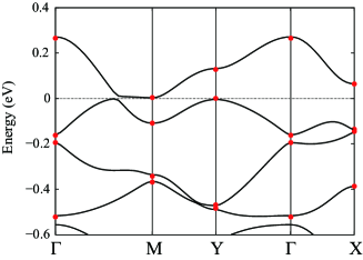
Figure 2: (Color online) Band structures including SOC effect along with the symmetric points in the first Brillouin zone, which denote time-reversal invariant momenta (TRIM) given by $\Gamma$ = (0,0,0), S (M) =$(\pi,\pi,0)$, Y=$(0,-\pi,0)$, and X =$(\pi,0,0)$. The 2D vector is defined as $\bm{k}=k_{x}(1,0)+k_{y}(0,1)$ = ($k_{x}$, $k_{y}$). The solid curves are obtained by the first-principles DFT method, while the symbols are obtained from the TB model with Table 1.  [38] The symbols agree with those from the DFT calculations (solid curves) within an energy scale of 0.01 eV. The energy zero is set to be the top of the valence bands [$\tilde{E}^{\rm SO}_{3}$($\bm{k}$) and $\tilde{E}^{\rm SO}_{4}$($\bm{k}$)].

Figure 3(a) shows two bands of $E_{1}(\bm{k})$ and $E_{2}(\bm{k})$ as the function of $\delta\bm{k}=\bm{k}-\bm{k}_{\rm D}$, where Dirac points are given by $\pm\bm{k}_{\rm D}=\pm(0.72,-0.58)\pi$ with an energy $\epsilon_{\rm D}$ = $\mu=0.1684$ corresponding to the three-quarter-filled band. The ranges of the energy of the conduction and valence bands $E_{1}(\bm{k})$ and $E_{2}(\bm{k})$ are given by $0<E_{1}(\bm{k})-\epsilon_{\rm D}<0.17$ and $-0.074<E_{2}(\bm{k})-\epsilon_{\rm D}<0$, respectively. Such ZGS shows the relation $E_{2}(Y)<\epsilon_{\rm D}<E_{1}(M)$, where $\Gamma$, X, Y, and M are TRIMs given by $\Gamma=(0,0)\pi$, $X=(1,0)\pi$, $Y=(0,1)\pi$, and $M=(1,1)\pi$, respectively. Figure 3(b) shows contour plots of $E_{1}(\bm{k})-E_{2}(\bm{k})$ around $\bm{k}_{\rm D}$. The contour lines form anisotropic circles, suggesting that the velocity of the Dirac cone is large for $k_{x}$ direction. In fact, $E_{1}(\delta\bm{k})-E_{2}(\delta\bm{k})=2\bm{v}\cdot\delta\bm{k}$ for small $|\delta\bm{k}|$ gives $v_{x}=0.075$ and $v_{y}=0.053$, which are compared with those of $\alpha$-(ET)₂I₃ ( $v_{x}=0.053$ and $v_{y}=0.043$). [19, 29] Figure 3(c) shows $E_{1}(\bm{k})-\epsilon_{\rm D}$. The Dirac point is located at $(\delta k_{x},\delta k_{y})$ = (0,0). This contour suggests a tilted Dirac cone and shows a slight deviation from the ellipse. In terms of a tilting velocity $v_{t}$ and the corresponding velocity of the Dirac cone $V$, the tilting parameter is estimated as $\eta=v_{t}/V\simeq 0.8$, which is nearly the same as that of $\alpha$-(ET)₂I₃.[24] It is also found that the cone shows a slight rotation clockwise from the $k_{x}$ axis, in contrast to that of $\alpha$-(ET)₂I₃ under hydrostatic pressure. [29] Figure 3(d) shows $E_{2}(\bm{k})-\epsilon_{\rm D}$. The Dirac point is located at (0,0). The contour of $E_{2}(\bm{k})-\epsilon_{\rm D}$ also shows a tilted Dirac cone and a slight deviation from the ellipse. We define a phase $\phi_{1}(<0)$ ( $\phi_{2}$) as a tilting angle of $E_{1}(\bm{k})$ ($E_{2}(\bm{k})$) measured from the $k_{x}$ axis. Since $E_{1}(\bm{k})$ and $E_{2}(\bm{k})$ form a pair of Dirac cones, $\phi_{2}-\phi_{1}=\pi$ for $\bm{k}$ in the limit of the Dirac point. The deviation from the limiting value increases with increasing $|\delta\bm{k}|$. Figure 3(e) shows a bright color line of $E_{2}(\bm{k})+E_{1}(\bm{k})=2\epsilon_{\rm D}$, on which the Dirac point is located, i.e., the apex of the Dirac cone. Thus, the line is almost perpendicular to the tilting axis, which rotates clockwise from the $k_{x}$ axis as discussed later.

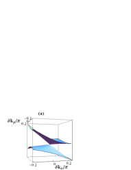
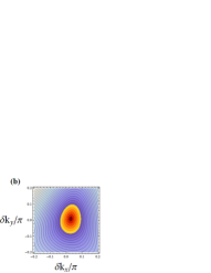
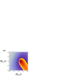
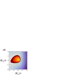
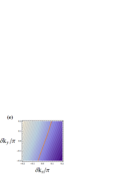
Figure 3: (Color online) (a) Conduction and valence bands given by $E_{1}(\bm{k})$ (upper band) and $E_{2}(\bm{k})$ (lower band). Two bands contact at the Dirac points $\pm\bm{k}_{\rm D}=\pm(0.72,-0.58)\pi$ with an energy $\epsilon_{\rm D}=\mu=0.1684$. Here we use $\delta\bm{k}=\bm{k}-\bm{k}_{\rm D}=(\delta k_{x},\delta k_{y})$. (b) Contour plots of $E_{1}(\bm{k})-E_{2}(\bm{k})(<0.144)$. The outermost bright line (OBL) corresponds to $E_{1}(\bm{k})-E_{2}(\bm{k})$ = 0.03. (c) Contour plots of $E_{1}(\bm{k})-\epsilon_{\rm D}$ with the range [0, 0.19], where the Dirac point exists at (0,0). The OBL corresponds to $E_{1}(\bm{k})-\epsilon_{\rm D}$ = 0.01. (d) Contour plots of $E_{2}(\bm{k})-\epsilon_{\rm D}$ with the range [-0.074, 0]. The Dirac point exists at (0,0). The OBL corresponds to $E_{2}(\bm{k})-\epsilon_{\rm D}$ = -0.01. (e) Contour plots of $E_{1}(\bm{k})+E_{2}(\bm{k})-2\epsilon_{\rm D}$ with the range [-0.0636, 0.0901]. The bright line denotes $E_{1}(\bm{k})+E_{2}(\bm{k})-2\epsilon_{\rm D}=0$.

Figure 4 shows DOS as a function of $\omega-\mu$, where the inset denotes the $T$ dependence of the chemical potential $\mu(T)$. $\mu$ is the chemical potential at $T$=0. The van Hove singularities exist at C [$E_{2}(Y)$], peaks below C ( an intermediate region between $\bm{k}_{\rm D}$ and Y), and A [$E_{1}(M)$]. With increasing $T$, $\mu$ varies almost linearly. The increase in $\mu$ occurs since the van Hove singularity below the chemical potential has a large peak compared with the above one. The DOS close to the chemical potential shows a linear dependence for $\omega-\mu$. However, the range is narrow compared with that expected from Figs. 3(a) and 3(b). Such a difference is ascribed to the effect of A ($E_{1}$(M)) for $\omega-\mu>0$ and the effect of C ($E_{2}$(Y)) for $\omega-\mu<0$. The energy at the respective TRIM is close to that at the Dirac point. Moreover, the former(latter) shows a singularity due to a saddle point (a maximum). The behavior at the C point is in contrast with that of $\alpha$-(ET)₂I₃, which exhibits a saddle point due to $E_{2}$(Y) being much lower than $E_{2}(\epsilon_{\rm D})$.

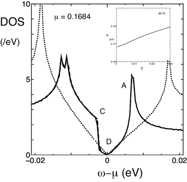
Figure 4: DOS as a function of $\omega-\mu=\omega$. The inset denotes chemical potential ($\mu$) as a function of temperature ($T$). The solid (dot-dashed) line represents DOS with (without) the imaginary part of the transfer energy. The dotted line corresponds to DOS for $\alpha$-(ET)₂I₃ under hydro-static pressure. [19]

Now we examine the conductivity and resistivity using Eqs. (LABEL:eq:sigma) and (14) with $\Gamma$ = 0.0005. We only calculate for the case of the SOC only with the same spin, i.e., by discarding $w_{s=-s^{\prime}}$, which results in the insulating gap of $\simeq$ 1 meV. Thus the present result is applied for $0.001<T$, where the resistivity enhancement at low temperature is still expected. First, we examine the case without the e–p interaction. Figures 5(a), 5(b) and 5(c) show the temperature dependence of conductivity of $\sigma_{\nu}$ ($\nu=x,y,xy,+,-$), $\sigma_{\nu}$ ($\nu=+,-$) and $1/\sigma_{\nu}$ ( = $\rho_{\nu}$), respectively. The case of transfer energy of only real part (dashed line) is compared with that of both real and imaginary parts (solid line).

In Fig. 5(a), one finds a relation $\sigma_{x}>\sigma_{y}$ for arbitrary $T$. This comes from the fact that the effect of the anisotropy of velocity, $v_{x}/v_{y}\simeq 1.4$ gives a significant effect compared with the tilting, $\eta\simeq 0.8$. This can be understood from a fact that the ratio of $\sigma_{x}/\sigma_{y}$ in the limit of the Dirac cone is proportional to a product of $(v_{x}/v_{y})^{2}$ and $\sqrt{1-\eta^{2}}\eta^{-1}\sin^{-1}\eta$. [26] Since $\sigma_{\nu}$ obtained for transfer energy in the presence of the imaginary part (solid line) is smaller than that with only real part (dashed line), it turns out that the SOC reduces the conductivity. In the presence of SOC ( solid curve), the difference between $\sigma_{x}$ and $\sigma_{y}$ at low temperature becomes negligibly small while the case without SOC (dashed line) shows a clear difference even at low temperature as seen also in the case of $\alpha$-(ET)₂I₃.[29]

In Fig. 5(b), principal values $\sigma_{\pm}$ are shown. The inset denotes the rotation angle $\phi$ of $\sigma_{+}$ measured from the $y$ axis. Note that the axis for $\sigma_{+}$ is perpendicular to the axis of the cone when the velocity of the cone is isotropic. [26] However $\phi/\pi(<-0.25)$ in the inset shows that there is a large deviation of the axis of $\sigma_{+}$ from that expected by the tilting (see Fig. 3(c)). This suggests $\sigma_{+}$, which is mainly determined by the anisotropy of the velocity, i.e., $v_{x}>v_{y}$. The axis for $\sigma_{+}$ rotates clockwise in accordance with $\sigma_{xy}>0$. It is found that $\sigma_{+}\simeq\sigma_{x}$ and $\sigma_{-}\simeq\sigma_{y}$ due to small $\sigma_{xy}$. Thus the magnitude of the dominant conductivity is given by $\sigma_{x}$, and the direction is relatively close to the $x$-direction. We note that $\sigma_{+}$ at low temperatures is convex downward, which contrasts that of $\alpha$-(ET)₂I₃. This is understood from the comparison between the solid line [$\alpha$-(BETS)₂I₃] and dotted line [$\alpha$-(ET)₂I₃] in Fig. 4, where the region of the linear dependence for DOS of $\alpha$-(BETS)₂I₃ is narrower than that of $\alpha$-(ET)₂I₃.

Figure 5(c) shows $T$ dependence of $1/\sigma_{\nu}$ ($\nu=x$ and $y$), where the dashed line corresponds to the transfer energy with an only real part. It increases gradually with decreasing temperature. The solid line corresponding to $1/\sigma_{\nu}$ with both real and imaginary parts shows a noticeable enhancement at low temperatures. The symbols denote $\rho_{\nu}$ ($\nu=x$ and $y$) obtained from Eq. (17). The difference between $1/\sigma_{\nu}$ and $\rho_{\nu}$ is negligibly small due to the small $\sigma_{xy}$.

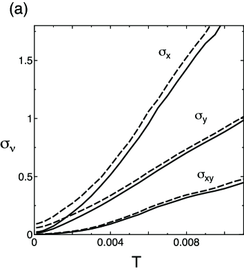
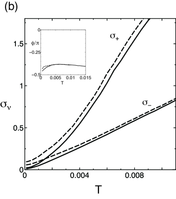
Figure 5: $T$ dependence of conductivity and resistivity in the absence of the e–p interaction with fixed $\Gamma$ = 0.0005. The dashed (solid) line corresponds to the case without (with) the imaginary part due to SOC. Figure 5(a) shows $\sigma_{x}$, $\sigma_{y}$, and $\sigma_{xy}$. Figure 5(b) shows $\sigma_{\pm}$. Principal values of $\sigma_{-}$ and $\sigma_{+}$ are given by Eqs. (16b) and (LABEL:eq:eq21c), respectively, while $\phi$ is given by Eq. (16a). The inset shows the phase $\phi$, which is an angle of the principal axis of $\sigma_{-}$ measured from the $k_{x}$ axis. Figure 5(c) shows the resistivity given by $1/\sigma_{\nu}$, where the symbol shows $\rho_{\nu}$ obtained from Eq. (17).

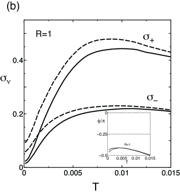
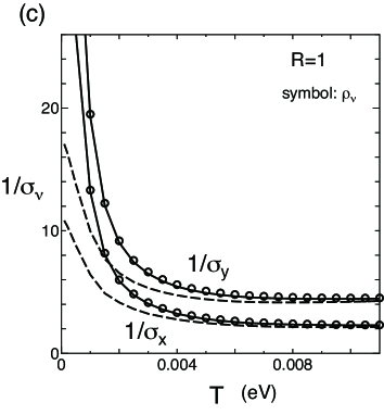
Figure 6: $T$ dependence of conductivity and resistivity in the presence of the e–p interaction with fixed $\Gamma$ = 0.0005. The normalized e–p coupling constant is taken as $R$=1, which is defined by Eq. (13b). The dashed (solid) line corresponds to the case without the SOC (with the SOC). Figure 6(a) shows $\sigma_{x}$, $\sigma_{y}$, and $\sigma_{xy}$. Figure 6(b) shows $\sigma_{\pm}$. The inset shows the phase $\phi$, which is an angle of the principal axis of $\sigma_{-}$ measured from the $k_{x}$ axis. Figure 6(c) shows the resistivity given by $1/\sigma_{\nu}$, where the symbol shows $\rho_{\nu}$ obtained from Eq. (17).

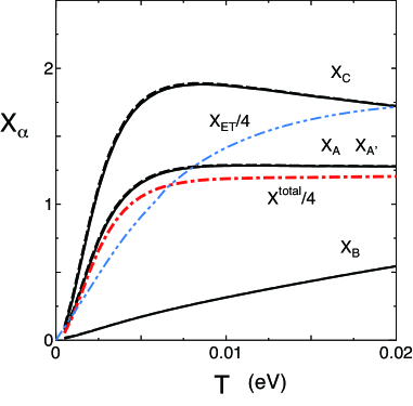
Figure 7: (Color online) Local magnetic susceptibility for A(=A’), B, and C molecular sites. The dashed line (solid line) is obtained for the transfer energy with real (complex). The dot-dashed line denotes $\chi^{\rm total}/4$ given by Eq. (20). The 2 dot-dashed line ($\chi_{\rm ET}$) corresponds to $\chi^{\rm total}$ for $\alpha$-(ET)₂I₃, [19] which is compared with that for BETS (dot-dashed line).

As shown in Fig. 5(a), $\sigma_{\nu}$ increases monotonically as a function of $T$, while the conductivity shows nearly constant at high temperatures.  [10] Such an exotic $T$ dependence of $\sigma_{\nu}$ is examined by taking account of the e–p interaction, which is expected to reduce $\sigma_{\nu}$. By using Eq. (29b) and (13a), we calculate $\sigma_{\nu}$ of Eq. (LABEL:eq:sigma), where $\Gamma$ in the absence of the e–p interaction is replaced by $\Gamma_{\gamma}(=\Gamma+\Gamma_{\rm ph}^{\gamma})$. Owing to the $T$ dependence of $\Gamma_{\rm ph}^{\gamma}$, $\Gamma$ is dominant at low $T$, whereas $\Gamma_{\rm ph}^{\gamma}$ is dominant at high $T$. Note that such crossover with increasing $T$ depends on $R$.

Figure 6(a) shows the $T$ dependence of $\sigma_{\nu}$ ($\nu=x,y,$ and $xy$) in the presence of the e–p interaction with a choice of $R=1$. The effect of the e–p interaction appears when $\sigma_{\nu}$ deviates from the $T$-linear behavior. Compared with $\sigma_{\nu}$ with $R$ = 0 (Fig. 5(a)), $\sigma_{\nu}$ is reduced noticeably. At temperatures above $T\sim 0.008$, $\sigma_{x}$ becomes nearly constant, while $\sigma_{y}$ shows such behavior at lower temperatures. Such a constant behavior of the conductivity is understood as follows. With increasing $T$, $\sigma_{\nu}$ without the e–p interaction ($R=0$) increases linearly owing to the DOS obtained from the Dirac cone. For $R\not=0$, the linear increase is suppressed at finite temperatures, since the effect of the acoustic phonon increases with increasing temperatures. The electron is scattered by both normal impurity ($\Gamma$) and the e–p interaction ($\Gamma_{\rm ph}^{\gamma}$), and the latter becomes dominant at high temperatures as seen from Eq. (13a). However, for the case of the Dirac cone close to the three-quarter-fil led band, the effect of the e–p scattering is strongly reduced owing to a constraint by the energy-momentum conservation.[28] Thus a nearly constant behavior or a broad maximum in $\sigma_{\nu}$, is obtained owing to a competition between the enhancement by DOS and the suppression by the e–p interaction in the Dirac electron system.

Here we mention the condition for $\Gamma_{\rm ph}$ of Eq. (13a), [28] which has been estimated for the acoustic phonon with an energy $v_{s}q$. Since the velocity $v_{s}$ of the acoustic phonon is much smaller than $v$ of Dirac cone, the energy-momentum conservation allows the classical treatment for a phonon distribution function due to $v_{s}q\ll vq\simeq T$. Furthermore, the numerical estimation shows that Eq. (13a) is proportional to the energy $\xi_{\bm{k},\gamma,s}$ for $|\xi_{\bm{k},\gamma,s}|/\Gamma_{0}<20$ with $\Gamma_{0}=0.005$, where the energy spectrum of the Dirac cone $\xi_{\bm{k},\gamma,s}$ is valid for $|\xi_{\bm{k},\gamma,s}|<0.015$ from Figs. 3 (b), (c) and (d). Thus, Eq. (13a) is valid for a region of $T<0.01$, in which the temperature corresponding to the maximum of the conductivity exists.

Figure 6(b) shows the $T$ dependence of $\sigma_{\pm}$, which is compared with Fig. 5(b). A broad maximum is seen in $\sigma_{+}$, and the almost constant behavior of $\sigma_{-}$ is similar to that of Fig. 5(b). Compared with the inset of Fig. 5(b), a maximum of the angle $\phi$ in the inset of Fig. 6(b) is seen due to a maximum in $\sigma_{xy}$. Such a maximum in the conductivity can be understood based on a simplified model, [28] where $\sigma_{+}\sim\sigma_{-}\sim\sigma$. Note that $\Gamma_{\rm ph}^{\gamma}$ is obtained in Eq. (13a) and $\sigma\simeq a_{\nu}^{\prime}10^{3}T/\Gamma$ with $a_{\nu}^{\prime}=o(0.1)$ without the e–p interaction. By taking $\Gamma$ replaced by $\Gamma+\Gamma_{\rm ph}^{\gamma}$ and employing an idea $<|\xi_{\gamma,\bm{k}}|>\sim T$ with $<>$ being an average value in the summation of Eq. (30) (Appendix B), we obtain

$$\sigma\simeq\frac{a_{\nu}^{\prime}10^{3}T}{1+C_{0}RT^{2}/\Gamma}\;,$$ (21)

with $C_{0}$ = 50 and $\Gamma$ = 0.0005. Equation (21) takes a maximum at $T=T_{m}=(\Gamma/C_{0}R)^{1/2}\simeq 0.003$, which is smaller than that of $\sigma_{+}$. Such $T_{m}$ can be improved by noting that $T$ in the numerator of Eq. (21) may be replaced by $T-\delta$ as seen from Fig. 5(b), e.g., $T_{m}\simeq 0.06$ for $\delta=0.002$. From Eq. (21), it is found that a maximum of $\sigma$ as a function of $T$ is obtained by a competition of the DOS (the numerator) and the e–p interaction (the denominator) and that $\sigma$ decreases with increasing $R$.

Figure 6(c) shows $T$ dependence of $1/\sigma_{\nu}$ ($\nu=x$ and $y$) for the transfer energy with real (dashed line) and complex (solid line). $T$ independent behavior of $1/\sigma_{\nu}$ is seen at high temperatures due to the e–p interaction and the gradual increase of $1/\sigma_{\nu}$ at low temperatures is similar to that of Fig. 5(c). The resistivity given by symbols, where the difference between the solid line and symbols are negligibly small, suggests the small effect of the e–p interaction on the off-diagonal component $\sigma_{xy}$. Since the effect of the e–p interaction is small for small $T$, the insulating behavior at low temperature comes from the SOC.

Finally, we examine spin susceptibility, which is evaluated from Eqs. (19) and (20). Figure 7 shows $T$ dependence of local magnetic susceptibility $\chi_{\alpha}$ ($\alpha$ = A, A’, B, and C), where the dashed line (solid line) is calculated for transfer energy with real (complex). The slight difference between the dash and real lines suggests that the reduction of the magnetic susceptibility by the SOC is negligibly small in contrast to the case of the conductivity. A relation $\chi_{A}=\chi_{A^{\prime}}$ holds due to the inversion symmetry around the middle of A and A’ sites. Compared with that of $\alpha$-(ET)₂I₃ , [19] the susceptibility of $\chi_{A}(=\chi_{A}^{\prime})$ and $\chi_{C}$ shows the rapid increase, while the linear behavior of $\chi_{B}$ is a common feature. The total susceptibility of $\alpha$-(BETS)₂I₃ ( $\chi^{\rm total}$) is shown by the dot-dashed line, which is compared with that for $\alpha$-(ET)₂I₃. [19] The noticeable increase for $\alpha$-(BETS)₂I₃ at finite temperatures is ascribed to a difference in DOS close to the chemical potential as shown in Fig. 4. We note the low temperature behaviors of $\chi$ in Fig. 7. For $\alpha$-(BETS)₂I₃, there is the following effect of the SOC on $\chi$. Since the calculation was performed only for $w_{h},s=s^{\prime}$, i.e., the transfer energy of the SOC with the same spin, the insulating gap ($\simeq$ 0.001 eV) due to the opposite spin is absent. However, compared with $\chi$ of $\alpha$-(ET)₂I₃, which represents $\chi_{\rm ET}\propto T$ in the absence of correlation, $\chi$ of $\alpha$-(BETS)₂I₃ shows a slight reduction from the linear dependence and is convex downward for $T\sim$0.0005. Although $\chi$ at lower temperatures is not shown due to the numerical accuracy, it is expected that $\chi$ reduces to zero linearly for $T\rightarrow 0$. Such a pseudogap behavior at low temperatures comes from the effect of the SOC with the same spin.

4 Summary and Discussion

We calculated the electric and magnetic properties of Dirac electrons in $\alpha$-(BETS)₂I₃ at ambient pressure and examined the similarity and dissimilarity with those of $\alpha$-(ET)₂I₃ at high pressures. [29] They show the common feature of almost temperature independent conductivity at high temperatures. The presence of the off-diagonal component ($\sigma_{xy}$), which is associated with both the tilting of the Dirac cone and anisotropy of the velocity, results in the rotation of the principal axis. The crucial difference is the SOC in $\alpha$-(BETS)₂I₃, which gives rise to the reduction of the conductivity (or the enhancement of the resistivity) at low temperatures. We obtained the anisotropic conductivity with $\sigma_{x}>\sigma_{y}$ due to the anisotropy of the velocity of the cone. In contrast the opposite relation $\sigma_{y}>\sigma_{x}$ is obtained for the previous case of the tilting along the $k_{x}$ -direction with almost isotropic velocity. [29] The DOS exhibits a linear dependence around the chemical potential. Still, such energy region is narrow compared with the previous case,  [29] since $\epsilon_{\rm D}$ is located close to the relevant TRIM at M and Y points. Thus the temperature region for the linear susceptibility becomes narrow.

Here, we compare our result with that of the experiment. The temperature dependence of resistance (corresponding to the inverse of the conductivity) shows a nearly constant behavior at high temperatures and noticeable increase at low temperatures. Our results are qualitatively consistent with those of the experiment under ambient pressure. [10] The enhancement at low temperatures comes from the interplay of the effects of the Dirac cone and the SOC. The SOC has a significant effect on the diagonal transfer energy with both real and imaginary parts. The present result is a possible mechanism for keeping an inversion symmetry between A and A’.

Recent measurement of resistivity of $\alpha$-(BETS)₂I₃ [34] shows an increase at ambient pressure but the almost constant behavior under pressure $\sim$ 0.55 GPa is quite similar to $\alpha$-(ET)₂I₃[14] suggesting Dirac fermion phase under pressure. Thus, under pressure, the effect of the SOC is reduced and the conventional Dirac cone is expected due to short range repulsive interaction.[8]

We calculated the spin susceptibility and found the rapid linear increase at low temperatures compared with that of $\alpha$-(ET)₂I₃.[19] Such a linear increase is compatible with a measurement under ambient pressure of the susceptibility in $\alpha$-(BETS)₂I₃. [44, 45] Although the rapid decrease of the susceptibility is found in $\alpha$-(ET)₂I₃ due to the effect of the long range Coulomb interaction, [21] the linear behavior in $\alpha$-(BETS)₂I₃ [44] suggests that such a correlation effect is small and the effect of the SOC is dominant for the insulating behavior.

Appendix A Matrix elements

Using first-principles calculations, the TB model is obtained as [38]

$$H_{0}=\sum_{i,j=1}^{N}\sum_{\alpha,\sigma}\sum_{\beta,\sigma^{\prime}}t_{i,j;\alpha,\beta;\sigma,\sigma^{\prime}}a^{\dagger}_{i,\alpha,\sigma}a_{j,\beta,\sigma^{\prime}}\;,$$ (22)

where $t_{i,j;\alpha,\beta;\sigma,\sigma^{\prime}}$ denotes a transfer energy obtained by $(\bf{j}-\bf{i}=\bf{R})$

$$t_{\alpha,\beta;\sigma,\sigma^{\prime}}(\mathbf{R})=\langle\phi_{\alpha,\sigma,0}|H|\phi_{\beta,\sigma^{\prime},\mathbf{R}}\rangle.$$ (23)

The quantity $\phi_{\alpha,\sigma,\mathbf{R}}$ is the MLWF spread over the molecule $\alpha$ and centered at $\mathbf{R}$. Equation (23) shows that $t_{i,j;\alpha,\beta;\sigma,\sigma^{\prime}}$ depends only on the difference between the $i$-th site and the $j$-th site.

We introduce site-potentials acting on $B$ and $C$ sites, $\Delta V_{B}$ and $\Delta V_{C}$, which are measured from site-energy at $A$ ($A^{\prime}$) site, $V_{A}$.[7]

$$\Delta V_{B}=V_{B}-V_{A},$$ (24)

$$\Delta V_{C}=V_{C}-V_{A},$$ (25)

where $V_{A}$, $V_{B}$, and $V_{C}$ are the site-energies at each molecule that are calculated using MLWFs $|\phi_{\alpha,0}\rangle$;

$$V_{\alpha}=\langle\phi_{\alpha,\sigma,0}|H|\phi_{\alpha,\sigma^{\prime},0}\rangle,$$ (26)

where ${\alpha}$ indicates $A$ (= $A^{\prime}$), $B$, and $C$ molecules. These site-potentials are listed in Table 1, where $\Delta V_{C}$ is modified from 0.0208 due to a correlation effect. [38] In terms of $X={\rm e}^{ik_{x}}$, $\bar{X}={\rm e}^{-ik_{x}}$, $Y={\rm e}^{ik_{y}}$, and $\bar{Y}={\rm e}^{-ik_{y}}$, matrix elements, $t_{ij}=(\hat{H})_{ij}$, are given by

$$t_{11} = t_{55}=a_{1d}(Y+\bar{Y})+s1X+s1^{*}\bar{X}\;,$$

$$t_{22} = t_{66}=a_{1d}(Y+\bar{Y})+s1^{*}X+s1\bar{X}\;,$$

$$t_{33} = t_{77}=a_{3d}(Y+\bar{Y})+s3(X+\bar{X})+\Delta V_{B}\;,$$

$$t_{44} = t_{88}=a_{4d}(Y+\bar{Y})+s4(X+\bar{X})+\Delta V_{C}\;,$$

$$t_{12} = t_{56}=a_{3}+a_{2}Y+d_{0}\bar{X}+d_{1}XY\;,$$

$$t_{13} = t_{57}=b_{3}+b_{2}\bar{X}+c_{2}\bar{X}Y+c_{4}\bar{X}\bar{Y}\;,$$

$$t_{14} = t_{58}=b_{4}Y+b_{1}\bar{X}Y+c_{1}\bar{X}+c_{3}\;,$$

$$t_{23} = t_{67}=b_{2}+b_{3}\bar{X}+c_{2}\bar{Y}+c_{4}{Y}\;,$$

$$t_{24} = t_{68}=b_{1}+b_{4}\bar{X}+c_{1}Y+c_{3}\bar{X}Y\;,$$

$$t_{34} = t_{78}=a_{1}+a_{1}Y+d_{2}\bar{X}+d_{3}X+d_{2}XY+d_{3}\bar{X}Y\;,$$

$$t_{17} = b2_{so1}\bar{X}+c2_{so1}\bar{X}Y+c4_{so1}\bar{X}\bar{Y}\;,$$

$$t_{18} = b1_{so1}\bar{X}Y+b4_{so1}Y+c1_{so1}\bar{X}\;,$$

$$t_{27} = b2_{so1}+c2_{so1}\bar{Y}+c4_{so1}Y\;,$$

$$t_{28} = b1_{so1}+c1_{so1}Y+c3_{so1}\bar{X}Y\;,$$

$$t_{35} = b2_{so2}X+c2_{so2}X\bar{Y}+c4_{so2}XY\;,$$

$$t_{36} = b2_{so2}+c2_{so2}Y+c4_{so2}\bar{Y}\;,$$

$$t_{45} = b1_{so2}X\bar{Y}+b4_{so2}\bar{Y}+c1_{so2}X\;,$$

$$t_{46} = b1_{so2}+c1_{so2}\bar{Y}+c3_{so2}X\bar{Y}\;,$$ (27)

$t_{15}=t_{16}=t_{25}=t_{26}=t_{37}=t_{38}=t_{47}=t_{48}=0$, and $t_{ji}=t_{ij}^{*}$.

Appendix B Damping by phonon scattering

For the electric transport, we calculate dampings of impurity and phonon scattering. In Eq. (1), the third term denotes the harmonic phonon given by $H_{\rm p}=\sum_{\bm{q}}\omega_{\bm{q}}b_{\bm{q}}^{\dagger}b_{\bm{q}}$ with $\omega_{\bm{q}}=v_{s}|\bm{q}|$ and $\hbar$ =1 ,and the fourth term is the e–p interaction expressed  [28]

$$H_{\rm e-p}=\sum_{\gamma,s}\sum_{\bm{k}}\sum_{\bm{q}}\alpha_{\bm{q}}c_{\gamma s}(\bm{k}+\bm{q})^{\dagger}c_{\gamma s}(\bm{k})\phi_{\bm{q}}\;,$$ (28)

with $\phi_{\bm{q}}=b_{\bm{q}}+b_{-\bm{q}}^{\dagger}$. We introduce a coupling constant $\lambda=|\alpha_{\bm{q}}|^{2}/\omega_{\bm{q}}$, which becomes independent of $|\bm{q}|$ for small $|\bm{q}|$. The e–p scattering is considered within the same band (i.e., intraband) owing to the energy conservation with $v\gg v_{s}$, where $v\simeq 0.05$ [19] denotes the averaged velocity of the Dirac cone. The last term of Eq. (1), $H_{\rm imp}$, denotes a normal impurity scattering, which gives a constant conductivity.

The damping of electrons of the $\gamma$ band, which is defined by $\Gamma_{\gamma}$, is obtained from the electron Green function[46] expressed as

$$G_{\gamma}(\bm{k},i\omega_{n})^{-1} = i\omega_{n}-E_{\gamma,\bm{k}}+\mu+i\Gamma_{\gamma}\;,$$ (29a)

$$\Gamma_{\gamma} = \Gamma+\Gamma_{\rm ph}^{\gamma}\;,$$ (29b)

where $\Gamma_{\rm ph}^{\gamma}=-{\rm Im}\Sigma_{\gamma}(\bm{k},E_{\gamma,\bm{k}}-\mu)$ with $\Sigma_{\gamma}(\bm{k},E_{\gamma,\bm{k}}-\mu)$ being a self-energy given by the e–p interaction. The real part of the self-energy can be neglected for doping at low concentrations. [28] The quantity $\Gamma$ comes from another self-energy by the impurity scattering. Note that $\Gamma_{\rm ph}^{\gamma}$ does not depend on $\Gamma$, and that the ratio $\Gamma_{\rm ph}^{\gamma}/\Gamma$ is crucial to the determination of the $T$ dependence of the conductivity. The quantity $\Sigma_{\gamma}(\bm{k},\omega)=\Sigma_{\gamma}(\bm{k},i\omega_{n})$ with $i\omega_{n}\rightarrow\omega+0$ is estimated from [46]

$$\Sigma_{\gamma}(\bm{k},i\omega_{n})=T\sum_{m}\sum_{\bm{q}}\;|\alpha_{q}|^{2}$$

$$\times\frac{1}{i\omega_{n+m}-\xi_{\gamma,\bm{k}+\bm{q}}}\times\frac{2\omega_{\bm{q}}}{\omega_{m}^{2}+\omega_{\bm{q}}^{2}}\;,$$ (30)

which is a product of electron and phonon Green functions. $\omega_{n}=(2n+1)\pi T$, $\omega_{m}=2\pi mT$ with $n$ and $m$ being integers. $\xi_{\gamma,\bm{k}}=E_{\gamma,\bm{k}}-\mu$. Applying the previous result,[28] we obtain Eqs. (13a) and (13b).

References

- [1] K. S. Novoselov, A. K. Geim, S. V. Morozov, D. Jiang, M. I. Katsnelson, I. V. Grigorieva, S. V. Dubonos, and A. A. Firsov, Nature 438, 197 (2005).
- [2] A. Kobayashi, S. Katayama, K. Noguchi, and Y. Suzumura, J. Phys. Soc. Jpn. 73, 3135 (2004).
- [3] S. Katayama, A. Kobayashi, and Y. Suzumura, J. Phys. Soc. Jpn. 75, 054705 (2006).
- [4] K. Kajita, Y. Nishio, N. Tajima, Y. Suzumura, and A. Kobayashi, J. Phys. Soc. Jpn. 83, 072002 (2014).
- [5] R. Kondo, S. Kagoshima, and J. Harada, Rev. Sci. Instrum. 76, 093902 (2005).
- [6] H. Kino and T. Miyazaki, J. Phys. Soc. Jpn. 75, 034704 (2006).
- [7] R. Kondo, S. Kagoshima, N. Tajima, and R. Kato, J. Phys. Soc. Jpn. 78, 114714 (2009).
- [8] T. Morinari and Y. Suzumura, J. Phys. Soc. Jpn. 83, 094701 (2014).
- [9] T. Naito, R. Doi, and Y. Suzumura, J. Phys. Soc. Jpn. 89, 023701 (2020).
- [10] M. Inokuchi, H. Tajima, A. Kobayashi, T. Ohta, H. Kuroda, R. Kato, T. Naito, and H. Kobayashi, Bull. Chem. Soc. Jpn. 68, 547 (1995).
- [11] K. Kajita, T. Ojiro, H. Fujii, Y. Nishio, H. Kobayashi, A. Kobayashi, and R. Kato, J. Phys. Soc. Jpn. 61, 23 (1992).
- [12] N. Tajima, M. Tamura, Y. Nishio, K. Kajita, and Y. Iye, J. Phys. Soc. Jpn. 69, 543 (2000).
- [13] N. Tajima, A. Ebina-Tajima, M. Tamura, Y. Nishio, and K. Kajita, J. Phys. Soc. Jpn. 71, 1832 (2002).
- [14] N. Tajima, S. Sugawara, M. Tamura, R. Kato, Y. Nishio, and K. Kajita, EPL 80, 47002 (2007).
- [15] D. Liu, K. Ishikawa, R. Takehara, K. Miyagawa, M. Tanuma, and K. Kanoda, Phys. Rev. Lett. 116, 226401 (2016).
- [16] Y. Takano, K. Hiraki, H. M. Yamamoto, T. Nakamura and T. Takahashi: J. Phys. Chem. Solids 62, 393 (2001).
- [17] R. Wojciechowskii, K. Yamamoto, K. Yakushi, M. Inokuchi and A. Kawamoto: Phys. Rev. B 67, 224105 (2003).
- [18] T. Kakiuchi, Y. Wakabayashi, H. Sawa, T. Takahashi, and T. Nakamura, J. Phys. Soc. Jpn. 76, 113702 (2007).
- [19] S. Katayama, A. Kobayashi, and Y. Suzumura, Eur. Phys. J. B 67, 139 (2009).
- [20] Y. Takano, K. Hiraki, Y. Takada, H.M. Yamamoto, and T. Takahashi, J. Phys. Soc. Jpn. 79, 104704 (2010).
- [21] M. Hirata, K. Ishikawa, K. Miyagawa, M. Tamura, C. Berthier, D. Basko, A. Kobayashi, G. Matsuno, and K. Kanoda, Nature Commun. 7, 12666 (2016).
- [22] A. Kobayashi, S. Katayama, Y. Suzumura, and H. Fukuyama, J. Phys. Soc. Jpn. 76, 034711 (2007).
- [23] M. O. Goerbig, J.-N. Fuchs, G. Montambaux, and F. Pichon, Phys. Rev. B 78, 045415 (2008).
- [24] A. Kobayashi, Y. Suzumura, and H. Fukuyama, J. Phys. Soc. Jpn. 77, 064718 (2008).
- [25] N. H. Shon and T. Ando, J. Phys. Soc. Jpn. 67, 2421 (1998).
- [26] Y. Suzumura, I. Proskurin, and M. Ogata J. Phys. Soc. Jpn. 83, 023701 (2014).
- [27] N. M. R. Peres, F. Guinea, and A. H. Castro Neto, Phys. Rev. B 83,125411 (2006).
- [28] Y. Suzumura and M. Ogata, Phys. Rev. B 98, 161205 (2018).
- [29] Y. Suzumura and M. Ogata, J. Phys. Soc. Jpn. 90, 044709 (2021).
- [30] K. Hiraki, S. Harada, K. Arai, Y. Takano, T. Takahashi, N. Tajima, R. Kato, T. Naito, J. Phys. Soc. Jpn. 80, 014715 (2011).
- [31] T. Shimamoto, K. Arai, Y. Takano, K. Hiraki, T. Takahashi, N. Tajima, R. Kato, and T. Naito, presented at JPS March Meeting, 2014.
- [32] S. Kitou, T. Tsumuraya, H. Sawahata, F. Ishii, K. Hiraki, T. Nakamura, N. Katayama, and H. Sawa, Phys. Rev. B 103, 035135 (2021).
- [33] P. Alemany, J.-P. Pouget, and E. Canadel, Phys. Rev. B 85, 195118 (2012).
- [34] Y. Kawasugi,H. Masuda, M. Uebe, H. M. Yamamoto, R. Kato, Y. Nishio, and N. Tajima, Phys. Rev. B 103, 205140 (2021).
- [35] S. Konschuh, M. Gmitra, and J. Fabian Phys. Rev. B 82, 245412 (2010).
- [36] S. Roychoudhury, and S. Sanvito, Phys. Rev. B 95, 085126 (2017).
- [37] S. M. Winter, K. Riedl, and R. Valenti, Phys. Rev. B 95, 060404(R) (2017).
- [38] T. Tsumuraya and Y. Suzumura, Eur. Phys. J. B 94, 17 (2020).
- [39] S. Katayama, A. Kobayashi, and Y. Suzumura, J. Phys. Soc. Jpn. 75, 023708 (2006).
- [40] V. N. Kotov, B. Uchoa, and V. M. Pereira, Rev. Mod. Phys. 84, 1067 (2012).
- [41] For example, see Eq. (6.9) in R. Kubo, J. Phys. Soc. Jpn. 12, 570 (1957).
- [42] A. A. Mostofi, J. R. Yates, G. Pizzi, Y. S. Lee, I. Souza, D . Vanderbilt, N. Marzari, Comput. Phys. Commun. 185, 2309 (2014)
- [43] P. Giannozzi and O. Andreussi and T. Brumme and O. Bunau and M. Buongiorno Nardelli and M. Calandra and R. Car and C. Cavazzoni and D. Ceresoli and M. Cococcioni and N. Colonna and I. Carnimeo and A. Dal Corso and S. de Gironcoli and P. Delugas and R. A. Di Stasio and A. Ferretti and A. Floris and G. Fratesi and G. Fugallo and R. Gebauer and U. Gerstmann and F. Giustino and T. Gorni and J. Jia and M. Kawamura and H-Y. Ko and A. Kokalj and E. Küçükbenli and M. Lazzeri and M. Marsili and N. Marzari and F. Mauri and N. L. Nguyen and H-V. Nguyen and A. Otero-de-la-Roza and L. Paulatto and S. Poncé and D. Rocca and R. Sabatini and B. Santra and M. Schlipf and A. P. Seitsonen and A. Smogunov and I. Timrov and T. Thonhauser and P. Umari and N. Vast and X. Wu and S. Baroni, J. Phys.: Condens. Matter 29, 465901 (2017).
- [44] S. Fujiyama, N. Tajima, and R. Kato, presented at JPS March meeting, 2021.
- [45] S. Fujiyama, H. Maebashi, N. Tajima, T. Tsumuraya, H-B Cui, M. Ogata, and R. Kato, cond-mat 2104.13547.
- [46] A. A. Abrikosov, L. P. Gorkov, and I. E. Dzyaloshinskii, Methods of Quantum Field Theory in Statistical Physics (Prentice-Hall, N.J., 1963).