Finite Element Method for Solution of Credit Rating Migration Problem Model

Abstract

In this paper, we propose a finite element method to study the problem of credit rating migration problem narrowed to a free boundary problem. Free boundary indeed separates the high and low rating region for a firm and causes some difficulties including discontinuity of second order derivative of the problem. Exploiting the weak formulation of the problem utilized in the Galerkin method, the discontinuity of second order derivative is averted. In this investigation we prove optimal convergence and stability of the proposed method. Numerical results illustrate how derived convergence results are consistent into practice ones.

[inst1]organization=Mississippi State University ,addressline=Center for Advanced Vehicular Systems (CAVS), city=Starkville, postcode=39759, state=MS, country=USA

1 Introduction

Over the recent years, quantitative credit risk modeling of financial institutions has been very popular in academia, industry and among regulators. Indeed, development of financial market of credit securities as well as standards offered by Basel accord have dramatically encouraged this interest. Default event, transition in the credit quality and variation of credit spreads are the main components of the credit risk modeling [1, 2]. Thus, developing efficient and accurate models and measures to identify and quantify credit is a necessity.

However, many investigations correspond credit risk with default risk which is the probability that a counterparty of a financial contract, either issuer of entities or a bank, does not meet the requirement of the contract. We learned the hard way due to the financial crisis that migration risk is also an intrinsic part of credit risk [3, 4]. Credit rating migration indicates that credit quality of a financial institution has upgraded or downgraded. It is well-known that these moves accelerated the eurozone’s sovereign debt crisis in 2010 and financial crisis of 2008.

A primary approach for the assessment of credit rating migration in the literature is utilizing the transition matrix of a Markov chain which consists of rating transition probabilities that an obligor migrates up or down to another rating [5, 6]. Former models benefit from the Markov property [5] that assumes that the predicted rating is independent from the rate history, whereas later models have been improved to be more realistic where they are exploiting various items such as the domicile of obligor and business cycle [7, 8, 9], and so forth.

The aforementioned approach is classified as a reduce-form method, which treats the rate migration exogenously without considering structural features of a firm such as asset and debt value of a company which can be essential in migrating a firm’s rate.

Some efforts have been made in the literature to broaden Merton method in order to employ the structural models in the purpose of modeling the value of a firm. Liang et al. [10, 11] used a boundary of high rating grade and low rating region obtained form real data using a statistical method as a threshold to determine whether the value of the firm is in a high rate region or a low rate region. The structural model developed with this threshold eventuates in a partial differential equation that has a close form solution under some proper boundary assumptions. However, this threshold is not anticipated in the real world, and later Bei Hu et al. [12] enhanced this model by assuming that the transition threshold is a proportion of structural variables of a firm like its debt and value. This model is then reduced to a free boundary value problem that explains credit rating migration of a firm where the threshold is a free boundary that is implicitly computed through time horizon. Hu and his colleagues in [12] proved that the solution of the derived free boundary problem exists and it is unique. Besides, they showed some regularity properties of the problem including free boundary. Later asymptotic traveling wave solution of a free boundary value problem for the problem of credit rating migration is investigated in [13]. In fact, they showed the existence and uniqueness of the solution of the problem, and using a construction proof benefit from Lyapunov function, they showed that the solution of the free boundary problem is convergent to the traveling wave solution. Yuan Wu et al. [14] studied valuation of a defaultable corporate bond with rating migration under a structural framework where there is a possibility of default apriorily at any time to maturity. They indeed used the first-passage-time model in which a barrier is the predetermined default threshold.

It is now widely known that the free boundary value problem derived from the migration problem, despite the fact of being well-posed, doesn’t have a closed form analytical solution. Thus, proposing efficient and accurate numerical methods that approximate the solution as well as the location of the free boundary is necessary. First a comprehensive study in this direction is performed in [15], where authors studied explicit finite difference scheme for numerical remedy of the free boundary problem. The convergence and stability of the method is analyzed in this work, and optimal convergence rate for spatial variable is derived. This finite difference method is proposed for the first time in [12] which corresponds to binomial tree scheme (BTS).

A variety of numerical methods has been exploited to deal with free boundary problems in the field of quantitative finance including finite difference method, finite element method, and recently introduced meshfree methods. However, among aforementioned methods, Galerkin method thanks to the framework of Hilbert space and Sobolev space is providing a suitable level of abstraction to perform error analysis of proposed schemes. Indeed, monitoring, measuring and controlling the error analysis of the Galerkin method have been broadly and extensively assessed in the field of engineering as well as quantitative finance over a relatively long time. Besides, developing, maintaining, and parallelizing the code for finite element method is trouble free in comparison to finite difference method for instance, and as a result it can lead to stronger and clearer error and convergence analysis. Therefore, we believe that investigating finite element for free boundary problem of migration rate problem is highly advantageous.

Finite element method is utilized to deal with free boundary problems obtained from American option in [16], where the exact discrete free boundary is derived using a stabilized algorithm. Allegretto, Lin and Yang [17] investigated error estimate of finite element method for solving free boundary problem of heat equation obtained by a change of variable in the problem of American option pricing. In fact, they studied the error analysis of variational inequality driven by the problem in a finite region. Holmesa and others in [18, 19] used front fixing finite element method for regime switching and American option with a variational inequality approach. The truncated free boundary value problem is directly computed through solving a nonlinear boundary value problem on a rectangular domain. They also performed the analysis of stability and positivity of the nonlinear system as well. Galerkin method with wavelet basis is used in [20] for dealing with free boundary problems of partial differential equations driven from American option on asset with Lévy price processes. Matche and others [20] benefited from the properties of wavelet basis to precondition the linear system arisen from the corresponding linear complementarity problem (LCP). Kovalov et al [21] used finite element to discretize the nonlinear PDE obtained form multi-asset American options penalized by a smooth penalty term. They solved the ODE system obtained form the discretization by an adaptive integrator. They also showed that non-smooth penalty improves the efficiency of the adaptive methodology. Furthermore, inverse finite element method is proposed in [22] to solve the nonlinear free boundary problem of American option without any linearization.

In this paper we develop the Galerkin method for dealing with migration rate problem. First we derive the weak formulation of the free boundary value problem which lessens the regularity requirement for the space of the solution. Since the boundary of the migration region brings discontinuity in the second order derivative, the weak form overcomes this discontinuity. A high order Lagrange finite element space is exploited to approximate the infinite space of the solution by the finite space. Error and stability analysis of the variational form of the parabolic free boundary problem is performed using some theoretical results for the associated elliptic problem. It is worth mentioning that some proofs or results depend on the known results for parabolic problems from the literature [23, 24, 25]. We tackle the free boundary value explicitly using green function and dual problem of the migration problem, and we propose a straight way to find the free boundary as well as the a priori estimation.

Let’s briefly review the outline of the remainder of this paper. 2 reviews the migration rate problem and presents the approximated system of equations for this problem. In section (3), we introduce the function spaces and notations we employ in this paper. Section (4) provides the weak formulation corresponding to the migration problem and some elementary properties of the bilinear form. In section (5), we ensure that the variational form presented is well-defined and has good regularity properties. Error analysis of approximating the problem in $L^{2}$ norm and $L_{\infty}$ are presented in section (7). Section (8) gives stability and convergence analysis of the proposed method. Utilizing green function and adjoint problems corresponding to the credit rating migration problem, an explicit method is proposed to estimate the free boundary. Section (10) shows numerical experiments and their results for the proposed method and error analysis.

2 Problem of Credit Rating Migration

Credit quality and default probability of a corporation is gauged by the bond rating. In this section, we review the structural model to value the bond so as to assess the problem of credit rating migration. Let’s assume that the firm issues solely a single zero-coupon bond with the face value $K$ which has a discount value of $\Phi_{t}$ at time $t$. Let $(\Omega,\mathcal{F},P)$ be a complete probability space, and $W_{t}$ is the Brownian motion adapted to the filtration of $\mathcal{F}$, the value of firm in the neutral world denoted by $S_{t}$ satisfies the following system:

$$dS_{t}=\left\{\begin{array}[]{ll}rS_{t}dt+\sigma_{H}S_{t}dW_{t},\quad\quad S_{t}\in\Omega_{H},\\ \\ rS_{t}dt+\sigma_{L}S_{t}dW_{t},\quad\quad S_{t}\in\Omega_{L},\end{array}\right.$$ (1)

where $r$ is the risk free interest rate, and the volatilities $\sigma_{H}<\sigma_{L}$ show the volatility of the firm in two regimes of low and high credit grades where high rating region and low rating region are shown by $\Omega_{H}$ and $\Omega_{L}$ respectively. Up region and low region are decided by the proportion of the debt and value of the firm with a threshold boundary which is represented by the constant $0<\nu<1$. Besides, it is trivial that if the maturity of the bound is in time $T$, the gain of an investor can be $\Phi_{T}=\min\{S_{T},K\}$ depending on the insolvency of the firm. One can show [26, 27] that $V_{H}(S_{t},t)$ and $V_{L}(S_{t},t)$ the values of bond in up and down grades with respect to the value of firm $S_{t}$ at time t satisfy the following system of PDEs with free boundary

$$\left\{\begin{array}[]{ll}\frac{\partial V_{H}}{\partial t}+\frac{1}{2}\sigma_{H}^{2}S^{2}\frac{\partial^{2}V_{H}}{\partial S^{2}}+rS\frac{\partial V_{H}}{\partial S}-rV_{H}=0,\quad S>\frac{1}{\nu}V_{H},\quad t>0,\\ \\ \frac{\partial V_{L}}{\partial t}+\frac{1}{2}\sigma_{L}^{2}S^{2}\frac{\partial^{2}V_{L}}{\partial S^{2}}+rS\frac{\partial V_{L}}{\partial S}-rV_{L}=0,\quad 0<S<\frac{1}{\nu}V_{L},\quad t>0,\\ \\ V_{H}(S,T)=V_{L}(S,T)=\min\{S,K\},\\ \\ \frac{\partial V_{H}}{\partial S}(s_{f},t)=\frac{\partial V_{L}}{\partial S}(s_{f},t),\quad s_{f}:\text{rating migration boundary}\\ \\ V_{H}(s_{f},t)=V_{L}(s_{f},t),\quad s_{f}:\text{rating migration boundary}\par\end{array}\right.$$ (2)

Using the standard change of variable $v(x,t)=V_{H}(e^{x},T-t)$ in high rating region and $v(x,t)=V_{L}(e^{x},T-t)$ in low rating region, switching to $x=\log\frac{S}{K}$, renaming $T-t=t$, and assuming without losing generality that the face value $K=1$, the following system of free boundary problems will be obtained

$$\left\{\begin{array}[]{ll}\frac{\partial v}{\partial t}-\frac{1}{2}\sigma_{H}^{2}\frac{\partial^{2}v}{\partial S^{2}}-(r-\frac{1}{2}\sigma_{H}^{2})\frac{\partial v}{\partial S}-rv=0,\quad v<{\nu}e^{x},\quad t>0,\\ \\ \frac{\partial v}{\partial t}-\frac{1}{2}\sigma_{L}^{2}\frac{\partial^{2}v}{\partial S^{2}}-(r-\frac{1}{2}\sigma_{L}^{2})\frac{\partial v}{\partial S}-rv=0,\quad v\geq{\nu}e^{x},\quad t>0,\\ \\ v(x,0)=\min\{S,1\},\\ \\ \lim_{x\to s_{f}^{-}}\frac{\partial v}{\partial S}(x,t)=\lim_{x\to(s_{f})^{+}}\frac{\partial v}{\partial S}(x,t),\\ \lim_{x\to s_{f}^{-}}v(x,t)=\lim_{x\to s_{f}^{+}}v(x,t)=\nu e^{s_{f}}.\end{array}\right.$$ (3)

Now, if we rewrite the volatilities in high and low rating regions as $\sigma=\sigma_{H}+(\sigma_{L}-\sigma_{H})H(v-\nu e^{x})$, where $H(x)$ is the Heaviside function, the following approximated system can be defined [12]

$$\left\{\begin{array}[]{ll}\frac{\partial v_{\epsilon}}{\partial t}+\mathcal{L}v_{\epsilon}=0\quad x\in\mathbb{R},\quad 0<t\leq T,\\ \\ v_{\epsilon}(x,0)=G(x),\quad x\in\mathbb{R},\\ \\ \sigma_{\epsilon}(v_{\epsilon}(x,t),t)=\sigma_{H}+(\sigma_{L}-\sigma_{H})H_{\epsilon}(v_{\epsilon}(x,t)-\nu e^{-\delta t})\end{array}\right.$$ (4)

in which the elliptic operator $\mathcal{L}v_{\epsilon}$ represents the following:

$$\mathcal{L}v_{\epsilon}=-\frac{1}{2}\sigma^{2}_{\epsilon}(v_{\epsilon}(x,t),t)\frac{\partial^{2}v_{\epsilon}}{\partial x^{2}}-\big{(}r+\frac{1}{2}\sigma^{2}_{\epsilon}(v_{\epsilon}(x,t),t)\big{)}\frac{\partial v_{\epsilon}}{\partial x},$$ (5)

the function $G(x)=\min\{1,e^{x}\}$, and $H_{\epsilon}$ is a $C^{\infty}$ function that approximates the Heaviside function (see [12] for more details), defined as follows:

$$\left\{\begin{array}[]{ll}H_{\epsilon}(x)=0,\quad x\leq-\epsilon\\ \\ H_{\epsilon}(x)=1,\quad x\geq 0,\\ \end{array}\right.$$ (6)

such that this function has these properties

$$0\leq H^{\prime}_{\epsilon}(x)\leq C\epsilon^{-1},\quad|H^{\prime\prime}_{\epsilon}(x)|\leq C\epsilon^{-2}.$$

The equation (4) has a unique solution [26] for every $\epsilon>0$. However, designing an efficient numerical solution of this equation due to the fact that the analytical solution is not available in hand is essential. In the proceeding sections, the proposed method to solve this free boundary value problem is presented.

3 Functional Spaces and Preliminaries

In this paper we assume $V$ is an infinite-dimensional function space where the weak formulation of equation (2) is defined, and it has the following form:

$$V:=H^{1}(\Omega)=\left\{u\in L^{2}(\Omega)\quad|\quad\frac{\partial u}{\partial x}\in L^{2}(\Omega)\right\},$$ (7)

where $\Omega$ is the spatial domain of the problem such that in one-dimension the truncated domain is $[x_{\min},x_{\max}]$, and $L^{2}(\Omega)$ is the Hilbert space of square integrable with the inner product $(\cdot,\cdot)$ defined as follows:

$$(u,v):=\int_{\Omega}uvdx,$$ (8)

with the induced norm $\|u\|_{L^{2}(\Omega)}=(u,u)^{\frac{1}{2}}$ . In the process of designing the finite element method to solve the weak formulation defined in the next section, infinite-dimension space $V$ is approximated by the space of continuous piecewise function $V_{h}$ on an element of $\Omega$ which is a finite dimension space. Indeed, functional space defined in (7) is a Sobolev space endowed with the norm

$$\|u\|_{H^{1}}=\left(\|u\|^{2}_{L^{2}(\Omega)}+\|\frac{\partial u}{\partial x}\|^{2}_{L^{2}(\Omega)}\right)^{\frac{1}{2}},$$ (9)

and semi-norm $|u|_{H^{1}}$ as follows:

$$|u|_{H^{1}}=\left(\|\frac{\partial u}{\partial x}\|^{2}_{L^{2}(\Omega)}\right)^{\frac{1}{2}},$$ (10)

accordingly, $H^{1}_{0}=H^{1}_{0}(\Omega)$ is the Sobolev space $H^{1}(\Omega)$ that vanishes outside of a compact support on $\partial\Omega$ boundary of the domain. However, we are using $\|.\|_{r}$ for norm of sobolev space of $H^{r}(\Omega)$ which one can find a detailed definition in [28].

4 Weak Formulation

In this sequence, we introduce the classical weak formulation corresponding to equation (4). By multiplying this equation (4) by a test function $v\in{V}$, and using the Green’s identity, the primal weak formulation of this problem is finding $u\in V$ such that

$$\left(\frac{\partial u}{\partial t},v\right)_{\Omega}+a(u,v)=0,\quad\forall v\in V,$$ (11)

where inner product of $L^{2}(\Omega)$ is denoted by $\left(\cdot,\cdot\right)$, and the bilinear form of $a(u,v):V\times V\xrightarrow{}\mathbb{R}$ is defined as follows:

$$a(u,v):=\left(\frac{1}{2}\sigma^{2}_{\epsilon}(u_{\epsilon}(x,t),t)\frac{\partial u_{\epsilon}}{\partial x},\frac{\partial v}{\partial x}\right)_{\Omega}+\left(\big{(}r+\frac{1}{2}\sigma^{2}_{\epsilon}(u_{\epsilon}(x,t),t)\big{)}\frac{\partial u_{\epsilon}}{\partial x},v\right)_{\Omega}+\langle\frac{\partial u_{\epsilon}}{\partial x},v\rangle_{\Gamma}+\langle u_{\epsilon},v\rangle_{\Gamma},$$ (12)

where $\Omega$ and $\Gamma$ are the domain and the boundary of the problem respectively, and $\langle\cdot,\cdot\rangle$ is the duality pair that realized $L^{2}(\Gamma)$ in the sobolev space. It is worth mentioning that $\sigma_{\epsilon}$ implicitly depends on the solution of the problem. However, it should be noted that if the test function $v\in H^{1}_{0}(\Omega)$ has a compact support which vanishes on the boundary, the last two terms of (12) will disappear.

4.1 Some Properties of the Bilinear Form

In this part we will look closely at the bilinear form of equation (12) and study some of its basic properties that will be used for analyzing the method in the next sections. But, first we drop the $\epsilon$ subscript for the sake of simplicity as a conventional notation in derived results. We commence with this observation that the bilinear form (12) is bounded, so as a result, it is continuous as well.

Lemma 4.1.

Let’s assume $X=H^{0}_{1}$ is the sobolev space of functions with compact support and $a:X\times X\longrightarrow\mathbb{C}$ is the bilinear form defined in (12), then we have

$$\|a(u,v)\|\leq C\|u\|_{1}\|v\|_{1}\quad\forall v\in H^{0}_{1}$$ (13)

where $C$ is a constant depend on the volatilises.

Proof.

To prove that (12) is bounded, one can observe that

$$\begin{array}[]{l}|a(u,v)|=|(\frac{1}{2}\sigma^{2}\frac{\partial u}{\partial x},\frac{\partial v}{\partial x})+((r+\frac{1}{2}\sigma^{2})\frac{\partial u}{\partial x},v)|\\ \end{array}$$

using the triangle inequality and some simple calculations we will have

$$\leq|(\frac{1}{2}\sigma^{2}\frac{\partial u}{\partial x},\frac{\partial v}{\partial x})|+|((r+\frac{1}{2}\sigma^{2})\frac{\partial u}{\partial x},v)|$$

now, using Cauchy-Schwarz inequality and assuming $C=\max\{(r+\frac{1}{2}\sigma_{L}^{2}),\frac{1}{2}\sigma_{L}^{2}\}$, and using sobolev embedding theorem [28] the desired result will be attained

$$\begin{array}[]{l}\leq\frac{1}{2}\sigma^{2}\|u\|_{1}\|v\|_{1}+|(r+\frac{1}{2}\sigma^{2})|\|\frac{\partial u}{\partial x}\|_{L_{2}}\|v\|_{L_{2}}\leq C\|u\|_{1}\|v\|_{1}.\end{array}$$

∎

The bilinear form (12) is not necessarily symmetric or positive definite depending on the value of volatilises and interest rate of the market. However, coercivity of this bilinear form can be shown as follows:

proposition 4.2 (Coercivity).

Let $u\in H^{1}_{0}$, then the bilinear form of 12 satisfies the following inequality:

$$a(u,u)\geq C_{1}\|u\|_{1}^{2}-C_{2}\|u\|^{2},\quad\forall u\in H^{1}_{0},\quad C_{1}\in\mathbb{R}^{+},C_{2}\in\mathbb{R}$$ (14)

where $C_{1}$ and $C_{2}$ are constants.

Proof.

For any $u\in H^{1}_{0}$, since $\|u\|_{L_{2}}$ is bounded, we can add this term to the bilinear form as follows:

$$\begin{array}[]{l}a(u,u)+C_{2}\|u\|^{2}_{L_{2}}\\ \\ \hskip 28.45274pt=(\frac{1}{2}\sigma^{2}\frac{\partial u}{\partial x},\frac{\partial u}{\partial x})+((r+\frac{1}{2}\sigma^{2})\frac{\partial u}{\partial x},u)+C_{2}(u,u)\\ \\ \hskip 28.45274pt=(\frac{1}{2}\sigma^{2}\frac{\partial u}{\partial x},\frac{\partial u}{\partial x})+(C_{2}-\frac{1}{2}(\frac{\partial(r+\sigma^{2})}{\partial x})u,u)\\ \\ \hskip 28.45274pt\geq C_{1}\|u\|^{2}_{1}\quad\text{if}\quad C_{2}>\sup{\frac{1}{2}(r+\frac{1}{2}\sigma^{2})}\end{array}$$

where $C_{1}=\min\{\frac{1}{2}\sigma_{H}^{2},C_{2}-\frac{1}{2}(r+\frac{1}{2}\sigma_{H}^{2})\}$ ∎

The inequality (14) is a G$\mathring{a}$rding type inequality that provides a lower bound for the elliptic bilinear form. Having the continuity and coercivity of the bilinear form (12), the existence and uniqueness of the solution of the variational form (11) can be shown [29] for any function belonging to Sobolev space $H^{1}_{0}(\Omega)$. Now, by proposition (4.2), obtaining result for the bilinear form of (12), we can investigate the stability of solution in the $L_{2}$-norm in chapter (5). At the end of this section we briefly mention the adjoint operator of the corresponding bilinear form (12) that we will use to find approximately the free boundary as well as the error of the numerical method. Let’s define an elliptic operator $L:H\xrightarrow{}\mathbb{C}$ as follows:

$$(Lu,v)=-({\frac{1}{2}\sigma^{2}}\frac{{{\partial^{2}}u}}{{\partial{x^{2}}}},v)-({(r+\frac{1}{2}\sigma^{2})}\frac{{\partial u}}{{\partial x}},v)$$ (15)

considering boundary condition of functions defined on the sobolev space $H^{1}_{0}$, we can define an adjoint operator $L^{*}:\mathbb{C}^{*}\xrightarrow{}H^{*}$ [30, 28, 31, 32] where

$$(u,{L^{*}}v)=-({\frac{1}{2}\sigma^{2}}u,v^{\prime\prime})+({(r+\frac{1}{2}\sigma^{2})}u,v^{\prime})\\$$ (16)

so, it is trivial that the operator $L$ is not self-adjoint. Using the corresponding adjoint problem defined on adjoint operator (16) of elliptic problem based on bilinear form (12), we first find the error of finite element method for the corresponding elliptic problem in the next chapter. Then, we use this error of the finite element approximation to assess the error of the finite element method for the main problem (11) in $L_{2}$ Norm. Besides, in chapter (9) the Green function and this adjoint problem are used to explicitly estimate the free boundary which separates the high volatility region from low volatility region.

5 Analysis of Variational Form

In this chapter we analyze the variational form introduced in (11), then an approximation of the variational form via a finite element space is investigated in the following section. The free boundary problem introduced in system (4) can be considered as a convection diffusion problem. It is well-known that numerical algorithms can be unstable when the convection term is dominated-that is-coefficient of second order derivative is relatively small. First we show that the variational form introduced is bonded, meaning that the solution is stable through time and it is not going to blow up to infinity.

proposition 5.1.

Solution of $u$ of variational form (11) satisfies the following stability estimate:

$$\|u(t)\|\leq\|G(x)\|+C,$$ (17)

where $C$ is a constant.

Proof.

First let’s choose $v=u$ in the variational form of (11) and some trivial calculations and integration, and having proposition (4.2) in hand we have

$$\begin{array}[]{l}(u_{t},u)=-a(u,u),\\ \\ \hskip 28.45274pt\frac{1}{2}\frac{d\|u\|^{2}}{dt}+C_{1}\|u\|^{2}_{1}\leq C_{2}\|u\|^{2},\\ \end{array}$$ (18)

and using Poincar$\acute{e}$ inequality for the first derivative we will have

$$\hskip 28.45274pt\frac{1}{2}\frac{d\|u\|^{2}}{dt}\leq C_{1}\|u\|^{2}+C_{2}\|u\|^{2},$$ (19)

now, integrating over time interval $[0,t]$ yields

$$\hskip 28.45274pt\|u(t)\|\leq\|G(x)\|+C_{2}\int_{0}^{t}\|u\|ds,$$ (20)

where the initial condition $G(x)$ is defined in chapter (2). Now, by using Gronwall’s lemma we will have

$$\hskip 28.45274pt\|u(t)\|\leq\|G(x)\|+C,$$ (21)

therefore, the desired result is attained. ∎

Although the boundedness of the solution is obtained from proposition(5.1), we can make the bound even sharper for this problem.

proposition 5.2.

Let’s assume solution $u\in H^{1}_{0}$ satisfies the variational equation (11), it is stable by the mean of being bounded with the following bound

$$\left\|{u(t)}\right\|\leq{C_{1}}\left\|{G(x)}\right\|+{C_{2}}\int_{0}^{t}{\left\|{\frac{{\partial u}}{{\partial x}}}\right\|}ds$$ (22)

where $C_{1}$ and $C_{2}$ are constants.

Proof.

First let’s again assume $u=v$ in the variational form (11), so we have

$$({u_{t}},u)+a(u,u)=0$$

In another word, we have the following variational equation:

$$\begin{array}[]{l}({u_{t}},u)+(\frac{1}{2}{\sigma^{2}}\frac{{\partial u}}{{\partial x}},\frac{{\partial u}}{{\partial x}})+((r+\frac{1}{2}{\sigma^{2}})\frac{{\partial u}}{{\partial x}},u)=0\\ \\ \frac{1}{2}\frac{d}{{dt}}{\left\|u\right\|^{2}}+{\frac{1}{2}{\sigma^{2}}}{\left\|{\frac{{\partial u}}{{\partial x}}}\right\|^{2}}+{|r+\frac{1}{2}{\sigma^{2}}|}(\frac{{\partial u}}{{\partial x}},u)=0\\ \end{array}$$

Using cauchy-shwartz for the second and third terms, we have

$$\begin{array}[]{l}\frac{d}{{dt}}{\left\|u\right\|^{2}}+{\sigma^{2}}{\left\|{\frac{{\partial u}}{{\partial x}}}\right\|^{2}}\leq 2{|r+\frac{1}{2}{\sigma^{2}}|}\left\|{\frac{{\partial u}}{{\partial x}}}\right\|\left\|u\right\|\par\end{array}$$

Now using Poincar$\acute{e}$ inequality, we will have

$$\frac{d}{{dt}}\left\|u\right\|+{\sigma^{2}}\left\|{\frac{{\partial u}}{{\partial x}}}\right\|\leq 2{|r+\frac{1}{2}{\sigma^{2}}|}\left\|{\frac{{\partial u}}{{\partial x}}}\right\|\\$$

If we multiply both sides of the above equation by ${e^{{\sigma^{2}}t}}$,

$$\frac{d}{{dt}}({e^{{\sigma^{2}}t}}\left\|u\right\|)+{{\sigma^{2}}}{e^{{\sigma^{2}}t}}\left\|{\frac{{\partial u}}{{\partial x}}}\right\|\leq 2{|r+\frac{1}{2}{\sigma^{2}}|}{e^{{\sigma^{2}}t}}\left\|{\frac{{\partial u}}{{\partial x}}}\right\|$$

the left hand side of the above equation can be written as a complete differential

$$\frac{d}{{dt}}({e^{{\sigma^{2}}t}}\left\|u\right\|)\leq 2{|r+\frac{1}{2}{\sigma^{2}}|}{e^{{\sigma^{2}}t}}\left\|{\frac{{\partial u}}{{\partial x}}}\right\|$$ (23)

By integration from both sides, the left hand side will have the following form:

$$\int_{0}^{t}{\frac{d}{{dt}}{e^{{\sigma^{2}}t}}\left\|u\right\|=\left\|{u(t)}\right\|}{e^{{\sigma^{2}}t}}-\left\|{u(0)}\right\|$$

So, by substituting the above integration in the inequality of (23), and some calculations

$$\left\|{u(t)}\right\|\leq{e^{-{\sigma^{2}}t}}\left\|{G(x)}\right\|+2{|r+\frac{1}{2}{\sigma(x)^{2}}|}\int_{0}^{t}{\left\|{\frac{{\partial u}}{{\partial x}}}\right\|}ds$$ (24)

now, assuming $C_{1}:=\sup\{{e^{-{\sigma(x)^{2}}t}}|\quad t\in[0,T],x\in\Omega=\Omega_{H}\cup\Omega_{L}\}$ and $C_{2}:=\sup\{{|r+\frac{1}{2}{\sigma(x)^{2}}|}\quad x\in\Omega=\Omega_{H}\cup\Omega_{L}\}$ the bound will derive, which shows that the solution is stable with the above upper bound (24). ∎

In this section, some stability properties of the variational form defined in (11) have been obtained. We showed that this form is well-defined and the solution of this variational form has an appropriate behavior for functions in the proper sobolev space $H^{1}_{0}(\Omega)$. Now, it is time to introduce the finite dimension approximation of this variational equation and study the accuracy and efficiency of the method.

6 Numerical Treatment with Finite Elements

In this section, we derive the primal formulation of credit rating migration problem from the variation form (11) using the standard Galerkin finite element method. Let $U_{h}$ be the finite element subspace of Sobolev space $H^{1}(\Omega)$ generated by piecewise polynomials of degree $\leq r$, and $V_{h}$ is the finite dimension subspace of test space $V$ where boundary terms vanish on $\partial\Gamma$. In this investigation we use continuous Galerkin method, that is, both finite subspace of trail space $H^{1}_{0}$ and subspace of test space $V$ overlaps meaning $V_{h}=U_{h}$. We define a partition $\mathcal{T}_{h}=\{T\}$ of sub-intervals such that $\Omega=\bigcup_{T\in T_{h}}T$, but not necessarily uniform of truncated spatial domain of $\Omega=[x_{min},x_{max}]$ such that $x_{min}\leq x_{1}\leq\cdots\leq x_{N_{s}}\leq x_{max}$, $h_{i}=x_{i+1}-x_{i}$ and $h=\max\{h_{i},i\in{1,\cdots,N_{s}}\}$. If we denote $u_{h}(t)=u(x_{h},t)$, where $x_{h}\in\mathcal{T}_{h}$, the primal formulation of the credit rating migration is finding $u_{h}(t)\in V_{h}$ such that

$$\left(\frac{\partial u_{h}}{\partial t},v_{h}\right)_{\Omega}+a_{h}(u_{h},v_{h})=0,\quad\forall v_{h}\in V_{h},$$ (25)

Where $a_{h}(u_{h},v_{h})$ is defined as approximate version of bilinear form as follows:

$$a_{h}(u_{h},v_{h}):=\left(\frac{1}{2}\sigma^{2}(u_{h}(x,t),t)\frac{\partial u_{h}}{\partial x},\frac{\partial v_{h}}{\partial x}\right)_{\Omega}+\left(\big{(}r+\frac{1}{2}\sigma^{2}(u_{h}(x,t),t)\big{)}\frac{\partial u_{h}}{\partial x},v_{h}\right)_{\Omega},$$ (26)

in fact, the equation (25) is semi-discrete and in order to fully approximate this equation numerically we discretize the time variable by the setting that $t_{n}=n\Delta t$ for $n\in\{1,\cdots,N_{t}\}$, where $\Delta t=\frac{T}{N_{t}}$, and applying backward Euler

$$\left(\frac{u^{n}_{h}-u^{n-1}_{h}}{\Delta t},v_{h}\right)_{\Omega}+a_{h}(u^{n}_{h},v_{h})=0,\quad\forall v_{h}\in V_{h},$$ (27)

where we used this notation convention $u^{n}_{h}:=u(x_{h},t_{n})$. However, volatilises are computed implicitly with respect to the data from the previous steps. Expanding the solution $u^{n}_{h}$ in a isoparametric form with the $N_{i}$ for $i\in\{1,\cdots,m\}$ of local piecewise continuous Lagrange shape functions of degree less than $p$ like $u^{n}_{h}(\xi)=\sum_{i=1}^{m}u_{i}N_{i}(\xi)$, where $\xi$ is the parent coordinate that can lead us to the following discrete system:

$$\left(\mathbf{K}+\Delta t\mathbf{M}\right)U^{n}=\mathbf{K}U^{n-1},$$ (28)

where vector $U^{n}=[u_{1},\cdots,u_{Ns}]^{T}$, $N_{s}$ unknown of degrees of freedom on domain $\Omega_{h}$, and $\mathbf{K}$ and $\mathbf{M}$ are stiffness and mass matrix corresponding with isoparametric form. It is not difficult to see that matrix on the left hand side of (28) is a positive definite and hence invertible [23].

7 Error Analysis of Finite Element Method

In this section, we analyze the approximate of the variational form in finite dimension space of the finite element space $V_{h}$. In order to show the error of approximation in $L_{2}$, first we use the standard duality argument invented by Nitsche and Aubin [33, 34] to find the error analysis of the corresponding elliptic problem, then using this approximation, we investigate the accuracy of the finite element approximation for free boundary value problem (4). Let’s recall the corresponding elliptic problem of variational form (11), this problem is seeking $u\in H^{1}_{0}$ which satisfies the following variation form:

$$a(u,v)=0,\quad\forall v\in V=H^{1}_{0},$$ (29)

where bilinear form is defined in (12). Now, if we use the approximation via the finite element space $V_{h}$ discussed in section (6), the discrete version of the problem (29) is finding $u_{h}\in V_{h}$ satisfying

$$a(u_{h},v_{h})=0,\quad\forall v_{h}\in V_{h},$$ (30)

now, let’s assess the accuracy of this approximation in $L_{2}$ norm.

proposition 7.1.

Assume $u_{h}\in V_{h}$ is satisfying (30) to approximate the solution of the corresponding elliptic problem (29), then

$${\left\|{u-{u_{h}}}\right\|_{L_{2}}}\leq C{h^{r+1}}{\left\|u\right\|_{r+1}}$$ (31)

and

$${\left\|{u-{u_{h}}}\right\|_{1}}\leq C{h^{r}}{\left\|u\right\|_{r+1}}$$ (32)

where $C$ is a constant.

Proof.

First, let’s recall the adjoint bilinear form introduced in section (4.1)

$${a^{*}}(u,u)=-({\frac{1}{2}{\sigma^{2}}}\frac{{\partial u}}{{\partial x}},\frac{{\partial v}}{{\partial x}})+({((r+\frac{1}{2}{\sigma^{2}})}u,\frac{{\partial v}}{{\partial x}}).$$

Assume if $\psi\in L^{2}(\Omega)$, we define $K(u):=\int_{\Omega}{u\psi dx}$, we can define the weak form of the dual problem pertain to (29) by seeking $\phi\in V$ such that

$${a^{*}}(w,\phi)=K(w)$$ (33)

Indeed, our adjoint problem is finding $\phi$ satisfying

$$\left\{\begin{array}[]{l}-{\frac{1}{2}{\sigma^{2}}}\frac{{\partial^{2}\phi}}{{\partial x^{2}}}+(r+\frac{1}{2}{\sigma^{2}})\frac{{\partial\phi}}{{\partial x}}=\psi,\quad\text{on}\quad\Omega,\\ \\ \phi(x,0)=G(x),\\ \\ \phi(x,t)=0,\quad\text{on}\quad x\in\partial\Omega,\end{array}\right.$$ (34)

Now we can define the error of approximating $K(u)$ by finite element space introduced in section (6) as follows:

$$K(u)-K({u_{h}})=\int_{\Omega}{(u-{u_{h}})\psi dx=-({{\frac{1}{2}{\sigma^{2}}}}\frac{{\partial(u-{u_{h}})}}{{\partial x}},\frac{{\partial\phi}}{{\partial x}})+({(r+\frac{1}{2}{\sigma^{2}})}(u-{u_{h}}),\frac{{\partial\phi}}{{\partial x}})},$$ (35)

using the definition of the adjoint operator, equation (35) equivalent to

$$K(u)-K({u_{h}})=-({\frac{1}{2}{\sigma^{2}}}\frac{{\partial(u-{u_{h}})}}{{\partial x}},\frac{{\partial\phi}}{{\partial x}})-({(r+\frac{1}{2}{\sigma^{2}})}\frac{{\partial(u-{u_{h}})}}{{\partial x}},\phi),\\$$

besides, with the Galerkin orthogonality we know

$$a(u-{u_{h}},\phi)=a(u-{u_{h}},\phi-v),$$

so, by the continuity of the bilinear form one can show that

$$\left|{K(u)-K({u_{h}})}\right|\leq C{\left\|{u-{u_{h}}}\right\|_{1}}\inf_{v\in V_{h}}{\left\|{\phi-v}\right\|_{1}},$$ (36)

by the regularity assumption on $\phi$, adjoint problem (34), and finite element error results (see [28] for more details) we get,

$$\inf_{v\in V_{h}}{\left\|{\phi-v}\right\|_{1}}\leq Ch{\left\|\phi\right\|_{1}}\leq Ch{\left\|\psi\right\|_{L^{2}}},$$

thus, the desired error (36) is shown as

$$\left|{K(u)-K({u_{h}})}\right|\leq Ch{\left\|{u-{u_{h}}}\right\|_{1}}{\left\|\psi\right\|_{L^{2}}}\leq c{h^{r+1}}{\left\|u\right\|_{r+1}}{\left\|\psi\right\|_{L^{2}}},$$ (37)

now, if we consider the special case of $\psi=u-u_{h}$, the error (36) will be

$$K(u)-K({u_{h}})=\int_{\Omega}{{{(u-{u_{h}})}^{2}}dx=}\left\|{u-{u_{h}}}\right\|_{L^{2}}^{2},\\$$ (38)

substituting the above result (38) in inequality (37) yields

$$\left\|{u-{u_{h}}}\right\|_{L^{2}}^{2}\leq Ch{\left\|{u-{u_{h}}}\right\|_{1}}{\left\|{u-{u_{h}}}\right\|_{L^{2}}}\\$$

Therefore,

$${\left\|{u-{u_{h}}}\right\|_{L^{2}}}\leq Ch{\left\|{u-{u_{h}}}\right\|_{1}}\leq C{h^{r+1}}{\left\|u\right\|_{r+1}}$$ (39)

which proves the proposition. ∎

In this proposition we proved the error bound for elliptic problem corresponding to the free boundary value problem using the Aubin-Nitsche duality argument. Now, we use this result to find the error of the finite element method to approximate the solution of 4. It is worth noticing that the technique used for this error is a common method that one can find in standard sources [35, 23, 24].

proposition 7.2.

Assume that $u\in H^{1}_{0}$ is the solution of the free boundary value problem that satisfies the corresponding variational form (11), and $u_{h}\in V_{h}$ is the solution of the finite dimensional variational problem with finite element in (25), then

1. $${\left\|{u-{u_{h}}}\right\|_{\infty}}=O({h^{r+1}})$$ (40)

2. $${\left\|{u-{u_{h}}}\right\|_{L_{2}}}=O({h^{r}})$$ (41)

Proof.

Let’s choose $w_{h}$ as an elliptic projection of the exact solution $u$ given by

$${\rm{a(}}{{\rm{w}}_{h}}{\rm{,v)=a(u,v),\quad v}}\in{{\rm{V}}_{h}},\quad 0\leq t\leq T$$

In proposition (7.1) we studied the error of the finite element method approximating the elliptic operator as follows:

$$\begin{array}[]{l}{\left\|{u(t)-{w_{h}}(t)}\right\|_{L_{2}}}\leq C{h^{r+1}}{\left\|{u(t)}\right\|_{r+1}},\quad 0\leq t\leq T\\ \\ {\left\|{u(t)-{w_{h}}(t)}\right\|_{1}}\leq C{h^{r}}{\left\|{u(t)}\right\|_{r+1}},\quad 0\leq t\leq T\\ \end{array}$$ (42)

Now, we differentiate with respect to time from both sides, and we know that time differentiation of $u_{h}$ is elliptic projection of differentiation of $u$, so

$${\left\|{\frac{{\partial u(t)}}{{\partial t}}-\frac{{\partial{w_{h}}(t)}}{{\partial t}}}\right\|_{L_{2}}}\leq c{h^{r+1}}{\left\|{\frac{{\partial u(t)}}{{\partial t}}}\right\|_{r+1}},\quad 0\leq t\leq T$$ (43)

So, we have

$$(\frac{{\partial{w_{h}}(t)}}{{\partial t}},v)+a({w_{h}},v)=(\frac{{\partial{w_{h}}(t)}}{{\partial t}},v)+a(u,v)=(\frac{{\partial({w_{h}}-u)}}{{\partial t}},v),\quad{\rm{v}}\in{{\rm{V}}_{h}},\quad 0\leq t\leq T$$ (44)

If we assume $\nu_{h}=w_{h}-u_{h}$

$$(\frac{{\partial{\nu_{h}}(t)}}{{\partial t}},v)+a({\nu_{h}},v)=(\frac{{\partial({w_{h}}-u)}}{{\partial t}},v),\quad{\rm{v}}\in{{\rm{V}}_{h}},\quad 0\leq t\leq T$$ (45)

If we use the differential representative of the first inner product in (45), and use Cauchy-Schwarz for the right hand side, we get

$$\left\|{{\nu_{h}}}\right\|_{L_{2}}\frac{d}{{dt}}\left\|{{\nu_{h}}}\right\|_{L_{2}}+a({\nu_{h}},{\nu_{h}})=(\frac{{\partial({w_{h}}-u)}}{{\partial t}},{\nu_{h}})\leq\left\|{\frac{{\partial({w_{h}}-u)}}{{\partial t}}}\right\|_{L_{2}}\left\|{{\nu_{h}}}\right\|_{L_{2}}$$ (46)

Therefore with simplification as well as the error bound of the projection (43) we will have

$$\frac{d}{{dt}}\left\|{{\nu_{h}}}\right\|_{L_{2}}\leq\left\|{\frac{{\partial({w_{h}}-u)}}{{\partial t}}}\right\|_{L_{2}}\leq C{h^{r+1}}{\left\|{\frac{{\partial u(t)}}{{\partial t}}}\right\|_{r+1}}$$ (47)

by integrating the above equation form $0$ to $T$, we will get

$$\left\|{{\nu_{h}}(t)}\right\|_{L_{2}}\leq\left\|{{\nu_{h}}(0)}\right\|_{L_{2}}+\int_{0}^{T}(C{h^{r+1}}{\left\|{\frac{{\partial u(s)}}{{\partial s}}}\right\|_{r+1}})ds$$ (48)

if we assume $u(0)$ is regular enough and we chose the initial data $u_{h}(0)$ such that $\|u(0)-u_{h}(0)\|_{L_{2}}=O(h^{r+1})$, we have

$$\begin{array}[]{l}\left\|{{\nu_{h}}(0)}\right\|_{L_{2}}=\left\|{{w_{h}}(0)-{u_{h}}(0)}\right\|_{L_{2}}\leq\left\|{{w_{h}}(0)-u(0)}\right\|_{L_{2}}+\left\|{{u(0)}-{u_{h}}(0)}\right\|_{L_{2}}\\ \\ \hskip 56.9055pt\leq C{h^{r+1}}{\left\|{{u(0)}}\right\|_{r+1}}+\left\|{{u(0)}-{u_{h}}(0)}\right\|_{L_{2}}=O(h^{r+1})\end{array}$$ (49)

Now, by using the triangle inequality and both the results in $H^{1}$ and $L_{2}$ for the elliptic error estimate in (42) as well as the inequality of (49), we get the desired results.

∎

The proposition (7.2) obtains an error bound for approximation of the finite element approximation.

8 Stability and Convergence of the Finite Element Method

In this section we investigate the stability and convergence of the discrete finite element method for solving the free boundary value problem (4). The variational form (11) has been discretized in the finite element space in spatial dimension (25) which eventuated in a set of ordinary differential equations. Then, we used backward Euler discretization in time to fully discretize the problem. First, let’s study the stability of the method meaning that the solution is not going to blow up as time proceeds. In the following proposition we show that the discrete solution of $u_{h}$ is bounded so it is stable numerically.

proposition 8.1.

Let $u_{h}$ be the solution of the discrete system of (25), and volatility of the market satisfies in the following:

$$\sum\limits_{n=1}^{n}{\left[\sigma(u(t_{n},x))^{2}-\frac{\partial\sigma(u(t_{n},x))^{2}}{\partial x}\right]}\geq 0,$$ (50)

then, the finite element approximation is stable and we also have

$$\max_{1\leq n\leq M}{\left\|{{u^{n}}}\right\|_{{L_{2}}}\leq C\left\|{{u^{0}}}\right\|_{{L_{2}}}},$$ (51)

where $M$ is the total number of time steps for Euler method, and $C$ is a constant.

Proof.

Assume $u_{h}\in V_{h}$ is the solution of fully discrete variational form of (25). We use an implicit Backward Euler finite difference to approximate the time derivative. so, we get

$$(\frac{{{u^{n}}-{u^{n-1}}}}{{\Delta t}},v)+a_{h}({u^{n}},v,{\sigma(u(t_{n-1},x))})=0,\quad v\in\forall V.$$ (52)

Note that in equation (52), bilinear form is unconventional and to some extent, imprecisely using third argument to emphasize dependency of volatility to the previous time step at each time step. By some elementary calculations we will have

$$\begin{array}[]{l}({u^{n}},v)-({u^{n-1}},v)+\Delta ta_{h}({u^{n}},v,{\sigma(u(t_{n-1},x))})=0,\\ \\ ({u^{n}},v)-({u^{n-1}},v)+\Delta t[(\frac{1}{2}{{\sigma(u(t_{n-1},x))}^{2}}\frac{{\partial{u^{n}}}}{{\partial x}},\frac{{\partial v}}{{\partial x}})+((r+\frac{1}{2}{{\sigma(u(t_{n-1},x))}^{2}})\frac{{\partial{u^{n}}}}{{\partial x}},v)]=0.\\ \end{array}$$ (53)

Let’s write ${u^{n}}=\Delta t\frac{{{u^{n}}-{u^{n-1}}}}{{2\Delta t}}+\frac{{{u^{n}}+{u^{n-1}}}}{2}$, therefore the equation (53) can be rewritten as

$$(\frac{{{u^{n}}-{u^{n-1}}}}{{\Delta t}},\Delta t\frac{{{u^{n}}-{u^{n-1}}}}{{2\Delta t}})+(\frac{{{u^{n}}-{u^{n-1}}}}{{\Delta t}},\frac{{{u^{n}}+{u^{n-1}}}}{2})+a_{h}({u^{n}},v,{{\sigma(u(t_{n-1},x))}})=0,$$

utilizing the norm notation for inner products in Hilbet space, one gets

$$\frac{{\Delta t}}{2}{\left\|{\frac{{{u^{n}}-{u^{n-1}}}}{{\Delta t}}}\right\|^{2}}+\frac{{{{\left\|{{u^{n}}}\right\|}^{2}}-{{\left\|{{u^{n-1}}}\right\|}^{2}}}}{{2\Delta t}}+a_{h}({u^{n}},v,{{\sigma(u(t_{n-1},x))}})=0.$$ (54)

Now, let’s consider a special case of $v=u^{n}$ in equation (54), so the following equation will be attained

$$\frac{{\Delta t}}{2}{\left\|{\frac{{{u^{n}}-{u^{n-1}}}}{{\Delta t}}}\right\|^{2}}+\frac{{{{\left\|{{u^{n}}}\right\|}^{2}}-{{\left\|{{u^{n-1}}}\right\|}^{2}}}}{{2\Delta t}}+\frac{1}{2}{\sigma(u(t_{n-1},x))}^{2}\left|{{u^{n}}}\right|_{1}^{2}-\frac{\partial}{{\partial x}}(r+\frac{1}{2}{\sigma(u(t_{n-1},x))}^{2}){\left\|{{u^{n}}}\right\|^{2}}=0,\\$$ (55)

using Poincar$\acute{e}$-Friedrich inequality and considering the fact that a norm is always positive, the following inequality is valid

$$\frac{{{{\left\|{{u^{n}}}\right\|}^{2}}-{{\left\|{{u^{n-1}}}\right\|}^{2}}}}{{2\Delta t}}+\frac{1}{2}{\sigma(u(t_{n-1},x))}^{2}\left|{{u^{n}}}\right|_{1}^{2}-\frac{\partial}{{\partial x}}(r+\frac{1}{2}{\sigma(u(t_{n-1},x))}^{2}){\left\|{{u^{n}}}\right\|^{2}}\leq 0,$$ (56)

so, sobolev embedding theorem for the second term of equation (56) will give us

$$\left[{1+\Delta t\left({\frac{1}{2}{\sigma(u(t_{n-1},x))}^{2}-\frac{\partial}{{\partial x}}(r+\frac{1}{2}{\sigma(u(t_{n-1},x))}^{2})}\right)}\right]\left\|{{u^{n}}}\right\|_{{L_{2}}}^{2}\leq\left\|{{u^{n-1}}}\right\|_{{L_{2}}}^{2},$$ (57)

summing over all time steps through the time discretization, and assuming condition of (50), the proposition will be proved. ∎

We showed in proposition (8.1) that the solution of discrete system (25) obtained from discretization of spatial variable by finite element and finite difference in time variable is bounded, that is, the discrete solution is numerically stable. In the next step, we study the simultaneous behavior of both linear Lagrange finite element and first order finite difference approximation of time derivative of variational problem (25) related to the credit risk migration and how algorithm is converging.

proposition 8.2.

Let $u_{h}$ be the solution of the fully discrete system of (27) obtained by linear Lagrange finite element method on spatial variable and first order finite difference for time derivative, then we have

$$\max_{1\leq n\leq M}{\left\|{{u^{n}}-u_{h}^{n}}\right\|_{{L_{2}}}}\leq C({h^{2}}+\Delta t),$$ (58)

where $M$ is the total number of time steps for Euler method, and $C$ is a constant.

Proof.

Let’s start by assuming that $w_{h}$ is the solution of the corresponding elliptic operator (30) such that

$$a(w_{h},{v_{h}})=a(u,{v_{h}}),\quad\forall{v_{h}}\in{V_{h}},\\$$

we present the error $e^{n}_{h}:=e(u(x_{h},t_{n}))$ of approximating the solution of the variational form (25) as

$$e_{h}^{n}:={u^{n}}-u_{h}^{n}={\alpha^{n}}+{\beta^{n}},\\$$ (59)

where decomposition elements of ${\alpha^{n}}$, and ${\beta^{n}}$ are defined as follows:

$$\begin{array}[]{l}{\alpha^{n}}={u^{n}}-{w_{h}^{n}},\\ \\ {\beta^{n}}={w_{h}^{n}}-u_{h}^{n}.\\ \end{array}$$ (60)

Using duality argument presented in section (7) in proposition(7.1), we get the following error bound for the linear finite element estimate of elliptic projection

$${\left\|{{\alpha^{n}}}\right\|_{{L_{2}}}}\leq C{h^{2}}{\left|{{u^{n}}}\right|_{2}},$$ (61)

it is trivial that $\alpha$ also satisfies

$$a(\frac{{{\alpha^{n+1}}-{\alpha^{n}}}}{{\Delta t}},{v_{h}})=0,\quad\forall{v_{h}}\in{V_{h}}\\$$ (62)

so by the inequality of (61), we get

$${\left\|{\frac{{{\alpha^{n+1}}-{\alpha^{n}}}}{{\Delta t}}}\right\|_{{L_{2}}}}\leq Ch^{2}{\left|{\frac{{{u^{n+1}}-{u^{n}}}}{{\Delta t}}}\right|_{{2}}},$$ (63)

besides, for $n=0$ we can write,

$$({\beta^{0}},{v_{h}})=(e_{h}^{0},{v_{h}})-({\alpha^{0}},{v_{h}})=-({\alpha^{0}},{v_{h}}).$$ (64)

Now, let’s consider a special case of $v_{h}={\beta^{0}}$, by using Cauchy-Schwarz inequality we will have

$${\left\|{{\beta^{0}}}\right\|_{{L_{2}}}}\leq{\left\|{{\alpha^{0}}}\right\|_{{L_{2}}}}\leq\frac{{{h^{2}}}}{{{p^{2}}}}{\left|{{u^{n}}}\right|_{2}}.$$ (65)

It is not difficult to see that $\beta$ is satisfying the following:

$$(\frac{{{\beta^{n+1}}-{\beta^{n}}}}{{\Delta t}},{v_{h}})+a({\alpha^{n+1}},{v_{h}})=(\frac{{{u^{n+1}}-{u^{n}}}}{{\Delta t}}-\frac{{\partial{u^{n}}}}{{\partial t}}-\frac{{{\alpha^{n+1}}-{\alpha^{n}}}}{{\Delta t}},{v_{h}}),$$ (66)

by the same procedure we prove the stability result in proposition (8.1), one can show that (see more details about duality argument in [34, 33])

$$\max_{1\leq n\leq M}{\left\|{{\beta^{n}}}\right\|_{{L_{2}}}}\leq{\left[{\left\|{{\beta^{0}}}\right\|_{{L_{2}}}^{2}+\sum_{n=1}^{N_{t}-1}{\Delta t\left\|{{\vartheta^{n+1}}}\right\|_{{L_{2}}}^{2}}}\right]^{{\raise 1.50694pt\hbox{$\scriptstyle 1$}\kern-0.70004pt/\kern-1.04996pt\lower 0.75346pt\hbox{$\scriptstyle 2$}}}},$$ (67)

where

$${\vartheta^{n+1}}:=\frac{{{u^{n+1}}-{u^{n}}}}{{\Delta t}}-\frac{{\partial{u^{n}}}}{{\partial t}}-\frac{{{\alpha^{n+1}}-{\alpha^{n}}}}{{\Delta t}}.$$ (68)

Since first term on the right hand side of (67) is estimated by the inequality of (65), so it remains to estimate the $\|{{\vartheta^{n+1}}}\|$, but we know from definition (68)

$${\left\|{{\vartheta^{n+1}}}\right\|_{{L_{2}}}}\leq{\left\|{\frac{{{u^{n+1}}-{u^{n}}}}{{\Delta t}}-\frac{{\partial{u^{n}}}}{{\partial t}}}\right\|_{{L_{2}}}}+{\left\|{\frac{{{\alpha^{m+1}}-{\alpha^{n}}}}{{\Delta t}}}\right\|_{{L_{2}}}}=I+II,$$ (69)

therefore, we need to assess the two components of (73). First term $I$ on the right hand side of the recent equation can be rewritten as

$$\frac{{{u^{n+1}}-{u^{n}}}}{{\Delta t}}-\frac{{\partial{u^{n}}}}{{\partial t}}=-\frac{1}{{\Delta t}}\int_{{t^{n}}}^{{t^{n+1}}}{(t-{t^{n}})\frac{{{\partial^{2}}{u^{n}}}}{{\partial{t^{2}}}}},$$ (70)

so we can show the following inequality for term $I$

$$I\leq\sqrt{\Delta t}{\left({\int_{{t^{n}}}^{{t^{n+1}}}{{{\left\|{\frac{{{\partial^{2}}{u^{n}}}}{{\partial{t^{2}}}}}\right\|}_{{L_{2}}}}}}\right)^{{\raise 2.1097pt\hbox{$1$}\!\mathord{\left/{\vphantom{12}}\right.\kern-1.2pt}\!\lower 2.1097pt\hbox{$2$}}}}.\\$$ (71)

inequality of (63) can be utilized for the second part $II$ of inequality (69)

$$II\leq Ch^{2}{\left|{\frac{{{u^{n+1}}-{u^{n}}}}{{\Delta t}}}\right|_{2}}=Ch^{2}{\left|{\frac{1}{{\Delta t}}\int_{{t^{n}}}^{{t^{n+1}}}{\frac{{\partial{u^{n}}}}{{\partial t}}}}\right|_{{2}}}\leq Ch^{2}\sqrt{\Delta t}{\left({\int_{{t^{n}}}^{{t^{n+1}}}{\left|{\frac{{\partial{u^{n}}}}{{\partial t}}}\right|}_{{2}}^{2}dt}\right)^{{\raise 2.1097pt\hbox{$1$}\!\mathord{\left/{\vphantom{12}}\right.\kern-1.2pt}\!\lower 2.1097pt\hbox{$2$}}}}.$$ (72)

By substituting the bound for $I$ and $II$, and using (67), and (65), we can find the bound for the $\beta$ a component of error in (59)

$$\max_{1\leq n\leq M}{\left\|{{\beta^{m+1}}}\right\|_{{L_{2}}}}\leq C1({h^{2}}+\Delta t),$$ (73)

but, the error term defined in (59) is compound of $\alpha$ and $\beta$, thus it implies that

$$\max_{1\leq n\leq M}{\left\|{{u^{n}}-u_{h}^{n}}\right\|_{{L_{2}}}}\leq\max_{1\leq n\leq M}{\left\|{{\beta^{n}}}\right\|_{{L_{2}}}}+\max_{1\leq n\leq M}{\left\|{{\alpha^{n}}}\right\|_{{L_{2}}}}.$$ (74)

Thus, by considering two bounds of (73),and (61) we will have the

$$\max_{1\leq n\leq M}{\left\|{{u^{n}}-u_{h}^{n}}\right\|_{{L_{2}}}}\leq C({h^{2}}+\Delta t).$$ (75)

which finishes the proof. In the end, it is worth noticing that constant $C$ is independent of $h$, and $\Delta t$ and it varies from constants defined in inequality (72) and (63) ∎

9 Dealing with Free Boundary

It is well-known that finding the free boundary where the volatility of firms switches between low and high credit grades is adding an extra complexity to the problem of rating migration. We must determine this boundary $S_{f}(t)$ where the solution $u(x,t)$ at each time $t$ reaches the value of $\gamma e^{-\delta t}$, where figure (1) illustrates figuratively this strategy. Besides finding this boundary value implicitly through solving the weak form and checking the occurrence of boundary value by ad-hoc method, we can estimate directly this free boundary value using green function and adjoint problem. To commence, we know that Green function $\varphi(s;x)$ for the system (4) satisfies in the following system of equations

$$\begin{array}[]{l}\left\{{\begin{array}[]{*{20}{l}}{{\varphi_{t}}+{L^{*}}\varphi={\delta_{s}}(x),\quad x\in\Omega},\\ \\ {\varphi(s;x)=0,\quad x\in\partial\Omega},\end{array}}\right.\\ \end{array}$$ (76)

where $L^{*}$ is the dual operator defined in (16), ${\delta_{s}}(x)$ is the delta function in $x$. It is easy to show that for each $s\in\Omega$ the solution of the weak form (11) satisfies the following:

$$u(s)=\int\limits_{\Omega}{{\delta_{s}}(x)}u(x)dx=\int\limits_{\Omega}{{\varphi_{t}}}u(x)dx+\int\limits_{\Omega}{{\frac{1}{2}{\sigma^{2}}}\frac{{{\partial^{2}}\varphi}}{{{x^{2}}}}}u(x)dx+\int\limits_{\Omega}{{(r+\frac{1}{2}{\sigma^{2}})}\frac{{\partial\varphi}}{x}}u(x)dx,$$ (77)

now by setting $u(S_{f})=\gamma e^{-\delta t}$ we will find the following nonlinear equation of

$${F_{\varphi(x,t)}}(S_{f}):=\int\limits_{\Omega}{{\varphi_{t}}}u(x)dx+\int\limits_{\Omega}{{{\frac{1}{2}{\sigma^{2}}}}\frac{{{\partial^{2}}\varphi}}{{{x^{2}}}}}u(x)dx+\int\limits_{\Omega}{{(r+{\frac{1}{2}{\sigma^{2}}}})\frac{{\partial\varphi}}{x}}u(x)dx-\gamma{e^{-\delta t}}=0.$$ (78)

Indeed, at each time $t$ of time interval, boundary value $S_{f}(t)$ by estimating the unique root of the equation ${F_{\varphi(x,t)}}(s)=0$ will be determined with standard an iterative method such as damped Newton method of the form of

$$x_{t_{i},h}^{m+1}=x_{t_{i},h}^{m}-\frac{{F^{h}_{\varphi(x,t)}}(x_{t_{i},h}^{m})}{{F^{{}^{\prime}h}_{\varphi(x,t)}}(x_{t_{i},h}^{m})},$$ (79)

where $F^{h}_{\varphi(x,t)}$ is finite element discretization of the nonlinear system (78). Thus, this strategy can be used to explicitly approximate the free boundary of migration risk rate problem.

Figure 1: Symbolically finding free boundary in time step $t_{n}$

10 Numerical Results

In this section the efficiency and accuracy of the estimated methodology designed so far is examined by applying it on the example presented in [15]. We study the case when $r=0.5$, $\delta=0.005$, $\sigma_{L}=0.3$, $\sigma_{H}=0.2$, $F=1$, $\gamma=0.8$, $T=1$. It is known [26, 15] that there is no analytical solution for the free boundary value problem (4). Thus, we used the numerical solution of the (4) via explicit finite difference proposed in [15] as a benchmark in order to compare the efficiency of our method. We used the $\Delta t=1.0\times 10^{-6}$ and $\Delta x=1.0\times 10^{-7}$ for the time steps and space steps respectively to attain this benchmark. We use finite element space $V_{h}$ of degree $r$ as investigated in the previous sections. We use Lagrange basis for generating the finite element space and Guess quadrature rule for evaluating integrals. All the computations performed in MATLAB and linear system solved with backslash operator in MATLAB.

The errors that we compute here are $\|E\|_{L_{2}(\Omega)}=\|u-u_{h}\|_{L_{2}(\Omega)}$, $\|E\|_{L_{\infty}(\Omega)}=\|u-u_{h}\|_{L_{\infty}(\Omega)}$ and ,$\|E\|_{H_{1}(\Omega)}=\|u-u_{h}\|_{H_{1}(\Omega)}$, where the exact solution is obtained as explained beforehand. We approximate the space of solution with the Lagrange finite element space of order $r$ to study the accuracy of the high order finite element as well. Before proceeding further, let’s mention again that we are estimating the time derivative with the first order finite difference method.

Table (1) showcases the error of estimating the solution with the finite element of order $r=1,2,3$. Optimal order of convergence for approximating by a polynomial of order $r$ for $\|E\|_{\infty}$ is $r+1$, whereas the optimal order for $\|E\|_{L_{2}(\Omega)}$ is $r$ (see proposition of (7.2)). However, we have not derived any theory about error in $H1$-norm, but numerical experiment shows that as we expect this accumulative error of solution and first derivative of solution is higher than the two other norm, but order is consistent with $L_{2}$-norm .that The order of convergence is consistent with the error estimate in (7.2)) and (8.2), and it is better than expected in high order estimation. For example when $r=3$, we see that $u_{h}$ converges with $O(h^{9/2})$ which is better than the optimal estimate. However, the last column of table (1) depicts that the method is rather expensive in terms of computational time especially as the order of the finite element method increases.

Table 1: Convergence Analysis of Finite Element Method, $N_{e}$ is the number of elements, $r$ represent the order of Lagrange shape functions

$N_{e}$	r	$|E|_{L_{2}}$	$|E|_{H^{1}}$	$|E|_{L_{inf}}$	$Time(s)$
1024	1	$0.0167\times 10^{-3}$	$0.0558.\times 10^{-3}$	$0.0016\times 10^{-5}$	0.8148
512	1	$0.0335\times 10^{-3}$	$0.0995\times 10^{-3}$	0.0014$\times$ $10^{-5}$	0.955
256	1	$0.0674\times 10^{-3}$	0.2392 $\times$ $10^{-3}$	0.0280$\times$ $10^{-5}$	1.812
128	1	0.1352$\times$ $10^{-3}$	0.4253 $\times$ $10^{-3}$	0.0993$\times$ $10^{-5}$	2.336
64	1	0.2703$\times$ $10^{-3}$	0.8326$\times$ $10^{-3}$	0.3858$\times$ $10^{-5}$	2.336
1024	2	0.0004$\times$ $10^{-5}$	0.0013 $\times$ $10^{-5}$	0.0002$\times$ $10^{-8}$	0.814
512	2	0.0016$\times$ $10^{-5}$	0.0046 $\times$ $10^{-5}$	0.0001$\times$ $10^{-8}$	0.955
256	2	0.0065$\times$ $10^{-5}$	0.0223 $\times$ $10^{-5}$	0.0124$\times$ $10^{-8}$	1.812
128	2	0.0262$\times$ $10^{-5}$	0.0797 $\times$ $10^{-5}$	0.0836$\times$ $10^{-8}$	2.336
64	2	0.1048$\times$ $10^{-5}$	0.3141$\times$ $10^{-5}$	0.6654$\times$ $10^{-8}$	2.336
1024	3	0.0001$\times$ $10^{-9}$	0.0002. $\times$ $10^{-8}$	0.0000$\times$ $10^{-12}$	0.814
512	3	0.0012$\times$ $10^{-9}$	0.0014 $\times$ $10^{-8}$	0.0000$\times$ $10^{-12}$	0.955
256	3	0.0107$\times$ $10^{-9}$	0.0138 $\times$ $10^{-8}$	0.0018$\times$ $10^{-12}$	1.812
128	3	0.0976$\times$ $10^{-9}$	0.0983 $\times$ $10^{-8}$	0.0348$\times$ $10^{-12}$	2.336
64	3	0.8893$\times$ $10^{-9}$	0.7694$\times$ $10^{-8}$	0.7780$\times$ $10^{-12}$	2.336457

Table (2) illustrates the estimate solution for the linear finite element method verses the variate time steps. The optimal error convergence for error in $L_{2}$ norm is one (see proposition (8.2)). Besides, we try to experiment the time order for the $H_{1}$ norm with numerical simulations. Based on the result of the table (2), the estimated order $O(h^{1.091})$ is performing slightly better than the optimal order, whereas the estimate order for $H_{1}$ norm is less than one $O(h^{0.887})$. Finally, figure (2) illustrates the surface of the approximated solution with linear Lagrange finite element method.

Table 2: Convergence analysis of time step with finite element method, $N_{t}$ is number of time steps

$N_{t}$	$|E|_{L_{2}}$	$|E|_{H^{1}}$	Time(s)
1024	0.0035 $\times 10^{-5}$	0.0146 $\times 10^{-3}$	0.814
512	0.0130 $\times 10^{-5}$	0.0293 $\times 10^{-3}$	0.955
256	0.0484$\times 10^{-5}$	0.0694 $\times 10^{-3}$	1.812
128	0.1807$\times 10^{-5}$	0.2017 $\times 10^{-3}$	2.336
64	0.6750 $\times 10^{-5}$	0.2343 $\times 10^{-3}$	2.336

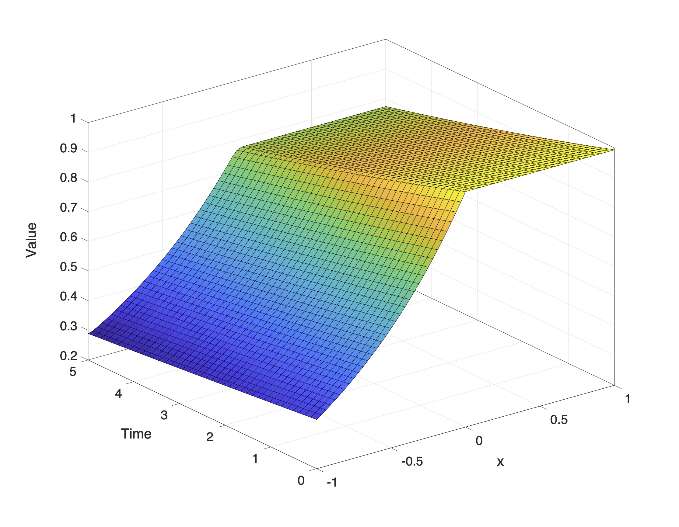
Figure 2: Approximated solution with linear finite element method

11 Conclusion

We showed that classic finite element method can be used to numerically solve the free boundary value problem arisen form the migration rate problem in credit risk study. The proposed variational form proposed in this paper is well-posed, that is the solution driven from this form is bounded. Analysis result about corresponding elliptic form of the problem assist in deriving convergence result for the numerical method for the free boundary value problem, although our estimates in this investigation are not always sharp. Benefiting form properties of adjoint problem and Green function, a direct method is devised to estimate the free boundary value problem. Numerical results showcased the quality of the proposed numerical methodology, and we saw better result in high order Lagrange finite element. in this work we assess the Backward Euler scheme, we may extend the method to the Crank-Nikolson scheme as well.

References

• [1] T. R. Bielecki, M. Rutkowski, Credit risk: modeling, valuation and hedging, Springer Science & Business Media, 2013.
• [2] A. J. McNeil, R. Frey, P. Embrechts, Quantitative risk management: concepts, techniques and tools-revised edition, Princeton university press, 2015.
• [3] A. Saunders, L. Allen, Credit risk management in and out of the financial crisis: new approaches to value at risk and other paradigms, Vol. 528, John Wiley & Sons, 2010.
• [4] W. K. Härdle, N. Hautsch, L. Overbeck, Applied quantitative finance, Springer Science & Business Media, 2008.
• [5] R. A. Jarrow, D. Lando, S. M. Turnbull, A markov model for the term structure of credit risk spreads, The review of financial studies 10 (2) (1997) 481–523.
• [6] S. R. Das, P. Tufano, Pricing credit sensitive debt when interest rates, credit ratings and credit spreads are stochastic (1995).
• [7] P. Nickell, W. Perraudin, S. Varotto, Stability of rating transitions, Journal of Banking & Finance 24 (1-2) (2000) 203–227.
• [8] D. Lando, T. M. Skødeberg, Analyzing rating transitions and rating drift with continuous observations, Journal of banking & finance 26 (2-3) (2002) 423–444.
• [9] U. Krüger, M. Stötzel, S. Trück, Time series properties of a rating system based on financial ratios, Tech. rep., Discussion Paper Series 2 (2005).
• [10] J. Liang, C. Zeng, Corporate bonds pricing under credit rating migration and structure framework, Applied Mathematics A Journal of Chinese Universities 30 (2015) 61–70.
• [11] J. Liang, Y. Zhao, X. Zhang, Utility indifference valuation of corporate bond with credit rating migration by structure approach, Economic Modelling 54 (2016) 339–346.
• [12] B. Hu, J. Liang, Y. Wu, A free boundary problem for corporate bond with credit rating migration, Journal of Mathematical Analysis and Applications 428 (2) (2015) 896–909.
• [13] J. Liang, Y. Wu, B. Hu, Asymptotic traveling wave solution for a credit rating migration problem, Journal of Differential Equations 261 (2) (2016) 1017–1045.
• [14] Y. Wu, J. Liang, B. Hu, A free boundary problem for defaultable corporate bond with credit rating migration risk and its asymptotic behavior, Discrete & Continuous Dynamical Systems-B 25 (3) (2020) 1043.
• [15] Y. Li, Z. Zhang, B. Hu, Convergence rate of an explicit finite difference scheme for a credit rating migration problem, SIAM Journal on Numerical Analysis 56 (4) (2018) 2430–2460.
• [16] W. Allegretto, Y. Lin, H. Yang, A fast and highly accurate numerical method for the evaluation of american options, Dynamics of Continuous, Discrete and Impulsive Systems Series B: Application and Algorithm 8 (1) (2001) 127–138.
• [17] W. Allegretto, Y. Lin, H. Yang, Finite element error estimates for a nonlocal problem in american option valuation, SIAM Journal on Numerical Analysis 39 (3) (2001) 834–857.
• [18] A. D. Holmes, H. Yang, S. Zhang, A front-fixing finite element method for the valuation of american options with regime switching, International Journal of Computer Mathematics 89 (9) (2012) 1094–1111.
• [19] A. D. Holmes, H. Yang, A front-fixing finite element method for the valuation of american options, SIAM journal on scientific computing 30 (4) (2008) 2158–2180.
• [20] A.-M. Matache*, P.-A. Nitsche, C. Schwab, Wavelet galerkin pricing of american options on lévy driven assets, Quantitative Finance 5 (4) (2005) 403–424.
• [21] P. Kovalov, V. Linetsky, M. Marcozzi, Pricing multi-asset american options: A finite element method-of-lines with smooth penalty, Journal of Scientific Computing 33 (3) (2007) 209–237.
• [22] S.-P. Zhu, W.-T. Chen, An inverse finite element method for pricing american options, Journal of Economic Dynamics and Control 37 (1) (2013) 231–250.
• [23] V. Thomée, From finite differences to finite elements a short history of numerical analysis of partial differential equations, Numerical Analysis: Historical Developments in the 20th Century (2001) 361–414.
• [24] J. Bramble, A. Schatz, V. Thomée, L. Wahlbin, Some convergence estimates for semidiscrete galerkin type approximations for parabolic equations, SIAM Journal on Numerical Analysis 14 (2) (1977) 218–241.
• [25] I. Babuska, M. Bieterman, The finite element method for parabolic equations. ii. a posteriori error estimation and adaptive approach, Numerische Mathematik 40 (1982) 373–406.
• [26] Y. W. B Hu, J Liang, A free boundary problem for corporate bond with credit rating migration, Journal of Mathematical Analysis and Applications 428 (2) (2015) 896–909. doi:https://doi.org/10.1016/j.jmaa.2015.03.040.
• [27] R. K. Dixit, A. K. Dixit, R. S. Pindyck, Investment under uncertainty, Princeton university press, 1994.
• [28] S. Brenner, R. Scott, The mathematical theory of finite element methods, Vol. 15, Springer Science & Business Media, 2007.
• [29] L. Evans, Partial differential equations graduate studies in mathematics vol 19 (american mathematical society: Providence, rhode island) (1998).
• [30] R. Vershynin, Lectures in functional analysis, Department of Mathematics, University of Michigan (2010).
• [31] D. Estep, A short course on duality, adjoint operators, green’s functions, and a posteriori error analysis, Lecture Notes (2004).
• [32] J. T. Oden, L. Demkowicz, Applied functional analysis, CRC press, 2017.
• [33] J. Nitsche, Lineare spline-funktionen und die methoden von ritz für elliptische randwertprobleme, Archive for Rational Mechanics and Analysis 36 (5) (1970) 348–355.
• [34] J. P. Aubin, Behavior of the error of the approximate solutions of boundary value problems for linear elliptic operators by galerkin’s and finite difference methods, Annali della Scuola Normale Superiore di Pisa-Classe di Scienze 21 (4) (1967) 599–637.
• [35] D. N. Arnold, Lecture notes on numerical analysis of partial differential equations (2012).