Using reinforcement learning to autonomously identify sources of error for agents in group missions

Abstract

When agents swarm to execute a mission, some of them frequently exhibit sudden failure, as observed from the command base. It is generally difficult to determine whether a failure is caused by actuators (hypothesis, $h_{a}$) or sensors (hypothesis, $h_{s}$) by solely relying on the communication between the command base and concerning agent. However, by instigating collusion between the agents, the cause of failure can be identified; in other words, we expect to detect corresponding displacements for $h_{a}$ but not for $h_{s}$. In this study, we considered the question as to whether artificial intelligence can autonomously generate an action plan $\bm{g}$ to pinpoint the cause as aforedescribed. Because the expected response to $\bm{g}$ generally depends upon the adopted hypothesis [let the difference be denoted by $D\left(\bm{g}\right)$], a formulation that uses $D\left(\bm{g}\right)$ to pinpoint the cause can be made. Although a $\bm{g}^{*}$ that maximizes $D\left(\bm{g}\right)$ would be a suitable action plan for this task, such an optimization is difficult to achieve using the conventional gradient method, as $D\left(\bm{g}\right)$ becomes nonzero in rare events such as collisions with other agents, and most swarm actions $\bm{g}$ give $D\left(\bm{g}\right)=0$. In other words, throughout almost the entire space of $\bm{g}$, $D\left(\bm{g}\right)$ has zero gradient, and the gradient method is not applicable. To overcome this problem, we formulated an action plan using Q-table reinforcement learning. Surprisingly, the optimal action plan generated via reinforcement learning presented a human-like solution to pinpoint the problem by colliding other agents with the failed agent. Using this simple prototype, we demonstrated the potential of applying Q-table reinforcement learning methods to plan autonomous actions to pinpoint the causes of failure.

I Introduction

The group cooperation of agents is an important topic studied in the context of autonomous systems. Lee et al. (2018); Hu et al. (2020) Because it is likely for each agent to have individual biases in its actuator or sensor performance, it is an important autonomous ability to analyze these inherent biases and revise the control plan appropriately to continue the group mission. Such biases dynamically vary during missions with time degradation, occasionally leading to the failure of some functionality in an agent. To ensure appropriate updates to the plan, the origins of such biases must be identified.

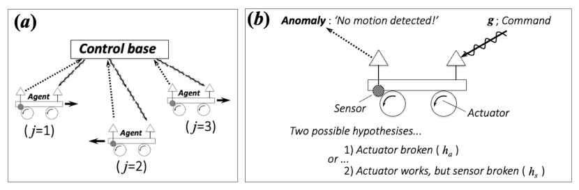
Figure 1: Agents perform group actions according to commands communicated from the “control base“ (the figure depicts an example with three agents indexed by $j$). The wavy arrow denotes a command signal from the base, whereas the dotted arrows represent the return signals from each sensor on each agent [panel (a)]. When an anomaly is detected in a return signal, two hypotheses - $h_{a}$ or $h_{s}$ - can be considered.

Suppose that a command base, which controls a group of agents via each command $g_{j}$ [Fig. 1 (a)] , has detected an anomaly in the position of an agent; (e.g., no change in the position was observed). There are two possible causes for the observed anomaly: (1) actuator failures (agent is unable to move,) or (2) sensor failures (agent can move, but the move is not captured by the sensor)  [Fig. 1 (b)] . Depending on the hypothesis, [the failure may have occurred in the actuators ($h_{a}$) or sensors ($h_{s}$)], the plan is subsequently calibrated and updated accordingly. However, it is generally difficult to identify which hypothesis caused the anomaly solely through communication between the base and agent. An intuitive method to identify the correct hypothesis is to execute a collision to the failure agent by other agents to check whether any displacement is observed by the sensor. Unless there is a case of sensor failure, such a collision would demonstrate agent displacement. Thus, the correct hypothesis can be identified by “planning a group motion“. The question then arises as to whether such planning can be set up autonomously as a “strategy to acquire environmental information“ Friston (2010).

Such autonomous planning appears to be feasible given the following value function. Suppose that the command $\bm{g}=\left(g_{1},g_{2},\cdots\right)$ is issued from the control base, directing the agent’s action to specify which of the hypotheses ($h_{a}$, $h_{s}$) is supported  [Fig. 1(a)]. This command updates the agent state to $\bm{R}\to\bm{\tilde{R}}\left({\bm{g}}\right)$. The updated state $\bm{\tilde{R}}$ should be denoted as $\bm{\tilde{R}}^{\left(h_{l}\right)}\left({\bm{g}}\right)$ because it depends on the hypothesis about the state before the update ($l=a,s$). As the expected results differ for different hypotheses, the following expression can be used to evaluate the distinction: $D=\left\|\bm{\tilde{R}}^{\left(h_{s}\right)}-\bm{\tilde{R}}^{\left(h_{a}\right)}\right\|$. To ensure appropriate planning $\bm{g}$ that involves collisions between agents, a non-zero difference $D$ is obtained and the likelihood of each hypothesis can be determined. We must therefore formulate a plan that maximizes $D=D\left({\bm{g}}\right)$ to ensure a significant difference. Accordingly, an autonomous action plan can be formulated to maximize $D\left({\bm{g}}\right)$ as a value function.

However, this maximization task is difficult to complete via conventional gradient-based optimization. Owing to the wide range of possibilities for $\bm{g}$, interactions such as collisions are rare events, and for most of the planning phase $\bm{g}$, $D\left({\bm{g}}\right)=0$, it is impossible to distinguish between hypotheses. Namely, sub-spaces with finite $D$ are sparse in the overall state space (sparse rewards). In such cases, gradient-based optimization is insufficient for the task of formulating appropriate action plans because the zero-gradient encompasses the vast majority of the space. For such sparse reward optimization, reinforcement learning, which has been thoroughly investigated in the applications of autonomous systems  Huang et al. (2005); Xia and El Kamel (2016); Zhu et al. (2018); Hu et al. (2020), can be used as an effective alternative.

Reinforcement learning  Nachum et al. (2018); Sutton and Barto (2018); Barto (2002) is becoming an established field in the wider context of robotics and system controls.  Peng et al. (2018); Finn and Levine (2017) Methodological improvements have been studied intensively, especially by verifications on gaming platforms.  Mnih et al. (2015); Silver et al. (2017); Vinyals et al. (2019) Thus, the topic addressed in this study is becoming a subfield known as multi-agent reinforcement learning (MARL).  Busoniu et al. (2006); Gupta et al. (2017); Straub et al. (2020); Bihl et al. (2020a); Gronauer and Diepold (2021) Specific examples of multi-agent missions include unmanned aerial vehicles (UAV)  Bihl et al. (2020a); Straub et al. (2020) and sensor resource management (SRM)  Malhotra et al. (2017, 1997); Hero and Cochran (2011); Bihl et al. (2020a). The objective of this study can also be regarded as the problem of handling non-stationary environments in multi-agent reinforcement learning.  Nguyen et al. (2020); Foerster et al. (2017) As a consequence of failure, agents are vulnerable to the gradual loss of homogeneity. Prior studies have addressed the problem of heterogeneity in multiagent reinforcement learning.  Busoniu et al. (2006); Calvo and Dusparic (2018); Bihl et al. (2020a); Straub et al. (2020); Gronauer and Diepold (2021) The problem of sparse rewards has also been recognized and discussed as one of the current challenges in reinforcement learning.  Wang and Taylor (2017); Bihl et al. (2020a)

As a prototype of such a problem, we considered a system composed of three agents moving on a ($x,y$)-plane, administrated by a command base to perform a cooperative task (Fig. 2). In performing the task, each agent is asked to convey an item to a goal post individually. The second agent (#2) is assumed to be unable to move along the $y$-direction due to actuator failure. By quickly verifying tiny displacements in each agent, the command base can detect the problem occurring in #2. However, it cannot attribute the cause to either the actuators or the sensors. Consequently, the control base sets hypotheses $h_{a}$ and $h_{s}$, and begins planning the best cooperative motions $\bm{g}^{*}$ to classify the correct hypothesis via reinforcement learning.

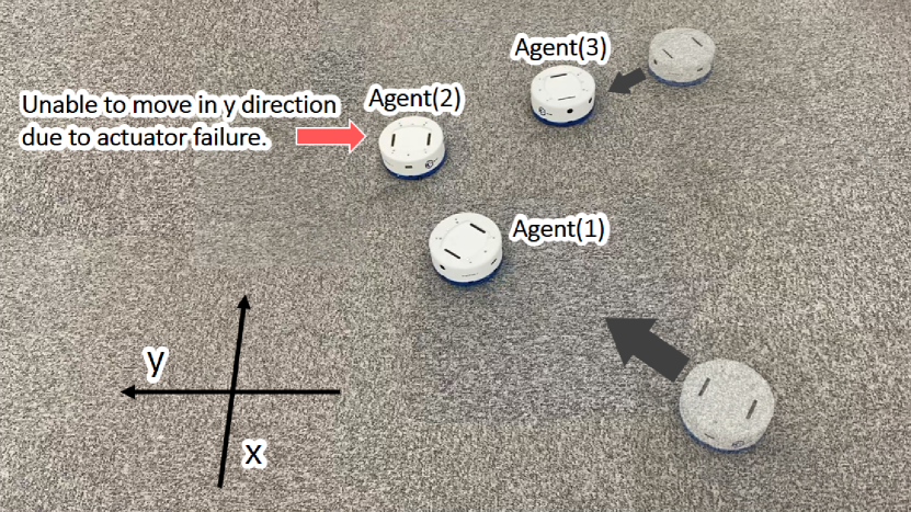
Figure 2: A view of actual machines labelled as Agents #1-#3. Agent #2 is unable to move in the y-direction due to actuator failure. Agents #1 and #3 are on their way to rescue Agent#2 (see main text about how the AI decides the action plan for the recovery of Agent #2).

Remarkably, the optimal action plan generated by reinforcement learning showed a human-like solution to pinpoint the problem by colliding other agents with the failed agent. By inducing a collision, the base could identify that #2 is experiencing problems with its actuators rather than sensors. The base then starts planning group motions to complete the conveying task considering the limited functionality of #2. We observe that the cooperative tasks are facilitated by a learning process wherein other agents appear to compensate for the deficiency of #2 by pushing it toward the goal. In the present study, we employed a simple prototype system to demonstrate that reinforcement learning is extremely effective in setting up a verification plan that pinpoints multiple hypotheses for general cases of system failure.

II Notations

Let the state space for the agents be ${\bm{R}}$. For instance, given three agents ($j=1,2,3$) situated on a $xy$-plane at positions $\left(x_{j},y_{j}\right)$, their states can be specified as ${\bm{R}}=\left(x_{1},y_{1},x_{2},y_{2},x_{3},y_{3}\right)$; i.e., points in six-dimensional space. The state is driven by a command ${\bm{g}}$ according the operation plan generated in the command base. When ${\bm{g}}$ is assigned to a given ${\bm{R}}$, the state is updated depending on which hypothesis $h_{l}$ is taken, each of which restricts ${\bm{R}}$ by individual constraint:

$${\bm{g}}:{\bm{R}}\to\tilde{\bm{R}}^{\left(h_{l}\right)}\left({\bm{g}},{\bm{R}}\right)\ .$$ (1)

The difference

$$D\left({\bm{g}},{\bm{R}}\right)=\sum_{<l,l^{\prime}>}{\left\|\tilde{\bm{R}}^{\left(h_{l}\right)}\left({\bm{g}},{\bm{R}}\right)-\tilde{\bm{R}}^{\left(h_{l^{\prime}}\right)}\left({\bm{g}},{\bm{R}}\right)\right\|}\ ,$$ (2)

can then be the measure to evaluate performance, and thereby distinguish between the hypotheses. The best operation plan for the distinction should therefore be determined as

$$\bm{g}^{*} = \mathop{\rm arg~{}max}\limits_{\bm{g}}D\left({\bm{g}},{\bm{R}}\right)\ .$$ (3)

The naive idea of performing optimization using gradient-based methods is insufficient owing to the sparseness described in the Introduction; For $\bm{g}$, $D(\bm{g},\bm{R})=0$, the gradient is zero for most of ${\bm{R}}$ because it is incapable of selecting the next update. Accordingly, we employed reinforcement learning as an alternative optimization approach.

Reinforcement learning assumes the value function $\rho\left({\bm{R}},{\bm{g}}\right)$, which measures the gain by taking the operation ${\bm{g}}$ for a state ${\bm{R}}$. The leaning process generates a decision that maximizes not the temporal $\rho\left({\bm{R}},{\bm{g}}\right)$, but also the long-standing benefit $Q\left({\bm{R}},{\bm{g}}\right)$, which is the approximate cumulative future gain. The benefit $Q$ is evaluated in a self-consistent manner (Bellman equation), as Sutton and Barto (2018)

$$Q\left({\bm{R}},{\bm{g}}\right) =\rho\left({\bm{R}},{\bm{g}}\right)$$

$$\quad+\sum_{{\bm{R}^{\prime}},{\bm{g}^{\prime}}}F\left(\left\{Q\left({\bm{R}^{\prime}},{\bm{g}^{\prime}}\right)\right\},\left\{\pi\left({\bm{R}^{\prime}},{\bm{g}^{\prime}}\right)\right\}\right)\ ,$$ (4)

where the second term sums all possible states (${\bm{R}^{\prime}}$) and actions (${\bm{g}^{\prime}}$) subsequent to the present choice $\left({\bm{R}},{\bm{g}}\right)$. The function $F\left(\left\{Q\left({\bm{R}^{\prime}},{\bm{g}^{\prime}}\right)\right\}\right)$ is composed as a linear combination over $\left\{Q\left({\bm{R}^{\prime}},{\bm{g}^{\prime}}\right)\right\}$, representing how the contributions get reduced over time. $\pi\left({\bm{R}},{\bm{g}}\right)$ in the second term $F$ describes the policy of taking the next decision $\bm{g}$ at state $\bm{R}$. As explained in Sec.VII.1, $\pi\left({\bm{R}},{\bm{g}}\right)$ is a probability distribution function with respect to $\bm{g}$, reflecting the benefit $Q\left(\bm{R},\bm{g}\right)$ as

$$\pi\left(\bm{R},\bm{g}\right)=P\left(Q\left(\bm{R},\bm{g}\right)\right)\ .$$

$Q\left({\bm{R}},{\bm{g}}\right)$ is regarded as in Table ($Q$-table) with respect to ${\bm{R}}$ and ${\bm{g}}$ as rows and columns. At the initial stage, all values in the table are set to random numbers and updated step by step by self-consistent iterations as follows: For the random initial values, the temporary decision for initial ${\bm{R}}_{0}$ is made formally by

$${\bm{g}}_{0}\sim\pi\left({\bm{R}}_{0},{\bm{g}}\right)\ ,$$

that is, the sampling by the random distribution at the initial stage. Given ${\bm{g}}_{0}$, a “point“ $\left({\bm{R}}_{0},{\bm{g}}_{0}\right)$ on the $Q$-table is updated from the previous random value as

$$Q\left({\bm{R}}_{0},{\bm{g}}_{0}\right) =\rho\left({\bm{R}}_{0},{\bm{g}}_{0}\right)$$

$$\quad+\sum_{{\bm{R}^{\prime}},{\bm{g}^{\prime}}}F\left(\left\{Q\left({\bm{R}^{\prime}},{\bm{g}^{\prime}}\right)\right\},\left\{\pi\left({\bm{R}^{\prime}},{\bm{g}^{\prime}}\right)\right\}\right)$$ (5)

where $\left\{Q\left({\bm{R}^{\prime}},{\bm{g}^{\prime}}\right)\right\}$ referred from the second term is still filled by the random number. The operation ${\bm{g}}_{0}$ then promotes the state to ${\bm{R}}_{0}\to{\bm{R}}_{1}$. Similar procedures are repeated for ${\bm{R}}_{1}$:

$${\bm{g}}_{1} \sim \pi\left({\bm{R}}_{1},{\bm{g}}\right)$$

$$Q\left({\bm{R}}_{1},{\bm{g}}_{1}\right) = \rho\left({\bm{R}}_{1},{\bm{g}}_{1}\right)$$

$$+\sum_{{\bm{R}^{\prime}},{\bm{g}^{\prime}}}F\left(\left\{Q\left({\bm{R}^{\prime}},{\bm{g}^{\prime}}\right)\right\},\left\{\pi\left({\bm{R}^{\prime}},{\bm{g}^{\prime}}\right)\right\}\right)$$

As such, the $Q$-table is updated in a patchwork manner as sensible values replace the initial random numbers. Assisted by the neural-network interpolation, values are filled for the whole range of the table, and then converged by the self-consistent iteration to get the final $Q$-table. In this implementation, a user specifies the form of $\rho\left({\bm{R}},{\bm{g}}\right)$, and $F\left(\left\{Q\left({\bm{R}}^{\prime},{\bm{g}}^{\prime}\right)\right\}\right)$, providing to the package. In this study, we used the OpenAI Gym Brockman et al. (2016) package.

Denoting the converged table as $\bar{Q}\left({\bm{R}},{\bm{g}}\right)$, we fix the policy as

$$\bar{\pi}\left(\bm{R},\bm{g}\right)=P\left(\bar{Q}\left(\bm{R},\bm{g}\right)\right)\ ,$$ (6)

to generate the series of operations for state updates:

$$\bar{\bm{g}}_{0} \sim \bar{\pi}\left({\bm{R}}_{0},{\bm{g}}\right)$$

$$\bar{\bm{g}}_{0}:{\bm{R}}_{0}\to{\bm{R}}_{1}$$

$$\bar{\bm{g}}_{1} \sim \bar{\pi}\left({\bm{R}}_{1},{\bm{g}}\right)$$

$$\bar{\bm{g}}_{1}:{\bm{R}}_{1}\to{\bm{R}}_{2}$$

$$\cdots \ .$$ (7)

III Experiments

The workflow required to achieve the mission for the agents, as described in Sec. Introduction, proceeds as follows:

• ] To determine if there are errors found in any of the agents, the base issues commands to move all agents by tiny displacements (and consequently, #2 is found to have an error).

• ] Corresponding to each possible hypothesis ($h_{a}$ and $h_{s}$), the virtual spaces $\left\{{\bm{R}}^{\left(h_{l}\right)}\right\}_{l=a,s}$ are prepared by applying each constraint.

• ]  Reinforcement learning ($Q_{\alpha}$) is performed at the command base using the virtual space, generating “the operation plan $\alpha$“ to distinguish the hypotheses.

• ]  The plan $\alpha$ is performed by the agents. The command base compares the observed trajectory with that obtained in the virtual spaces in Step [1]. In the process, the hypothesis that yields the closest trajectory to that observed is identified as accurate ($h_{a}$).

• ]  By taking the virtual space ${\bm{R}}^{\left(h_{a}\right)}$ as the identified hypothesis, another learning $Q_{\beta}$ is performed to get the optimal plan $\beta$ for the original mission (conveying items to goal posts).

• ]  Agents are operated according to the plan $\beta$.

All learning processes and operations are simulated on a Linux server. The learning phase is the most time-intensive, requiring approximately 3h using a single processor without any parallelization to complete. For the learning phase, we implemented the PPO2 (proximal policy optimization, version2) algorithm Schulman et al. (2015) from the OpenAI Gym Brockman et al. (2016) library. Reinforcement learning $(Q_{\alpha})$ was benchmarked on the MLP (multilayer perceptron) and LSTM (long-short time memory) network structures, with performance compared between them. We did not conduct specific tuning for the hyperparameters as a default setting, as shown in Table  1. However, it has been pointed out that hyperparameter optimization (HPO) can significantly improve the performance of reinforcement learning.  Henderson et al. (2018); Straub et al. (2020); Bihl et al. (2020b); Snoek et al. (2012); Domhan et al. (2015); Bihl et al. (2020a); Young et al. (2020) The comparison indicates that MLP performs better, with possible reasons given in the third paragraph of §IV. The results described herein Were obtained by the MLP network structure. Notably, LSTM also generated almost identical agent behaviors to those exhibited by the MLP (possible reasons are given in the Appendix, §VII.2.

Table 1: PPO2 hyperparameters used in training.

Parameter	Value
gamma	0.99
n_steps	128
ent_coef	0.01
learning_rate	0.00025
vf_coef	0.5
max_grad_norm	0.5
lam	0.95
nminibatches	4
noptepochs	4
cliprange	0.2

The learning process $Q_{\alpha}$ in step [1] is performed using two virtual spaces $V^{\left(h_{s},a\right)}$, corresponding to the two hypotheses

$${\bm{R}^{\left(h_{l}\right)}}\in V^{\left(h_{l}\right)}\ .$$ (8)

Each ${\bm{R}^{\left(h_{l}\right)}}$ can take such possibilities under each constraint of its hypothesis (e.g., $y_{3}$ cannot be updated due to the actuator error). For an operation ${\bm{g}}$, the state on each virtual space is updated as

$${\bm{g}}:\begin{array}[]{c}{\bm{R}}^{\left(h_{s}\right)}\to\tilde{\bm{R}}^{\left(h_{s}\right)}\left({\bm{g}},{\bm{R}}^{\left(h_{s}\right)}\right)\\ {\bm{R}}^{\left(h_{a}\right)}\to\tilde{\bm{R}}^{\left(h_{a}\right)}\left({\bm{g}},{\bm{R}}^{\left(h_{a}\right)}\right)\\ \end{array}\ .$$ (11)

Taking the value function,

$$\rho^{\left(\alpha\right)}\left({\bm{g}},{\bm{R}^{\left(h_{1}\right)}},{\bm{R}^{\left(h_{2}\right)}}\right)$$

$$={\left\|\tilde{\bm{R}}^{\left(h_{1}\right)}\left({\bm{g}},{\bm{R}^{\left(h_{1}\right)}}\right)-\tilde{\bm{R}}^{\left(h_{2}\right)}\left({\bm{g}},{\bm{R}^{\left(h_{1}\right)}}\right)\right\|}\ ,$$

the two-fold $Q$-table is updated self-consistently as

$$Q\left({\bm{g}},{\bm{R}^{\left(h_{1}\right)}},{\bm{R}^{\left(h_{2}\right)}}\right)$$

$$=\rho^{\left(\alpha\right)}\left({\bm{g}},{\bm{R}^{\left(h_{1}\right)}},{\bm{R}^{\left(h_{2}\right)}}\right)$$

$$\quad+\sum_{{\bm{g}^{\prime}},{\bm{R}^{\prime\left(h_{1}\right)}},{\bm{R}^{\prime\left(h_{2}\right)}}}F\left(\left\{Q\left({\bm{g}^{\prime}},{\bm{R}^{\prime\left(h_{1}\right)}},{\bm{R}^{\prime\left(h_{2}\right)}}\right)\right\},\right.$$

$$\quad\quad\quad\quad\quad\quad\quad\quad\quad\quad\quad\left.\left\{\pi\left({\bm{g}^{\prime}},{\bm{R}^{\prime\left(h_{1}\right)}},{\bm{R}^{\prime\left(h_{2}\right)}}\right)\right\}\right)\ .$$

Denoting the converged table as $\bar{Q}_{\alpha}\left({\bm{g}},{\bm{R}^{\left(h_{1}\right)}},{\bm{R}^{\left(h_{2}\right)}}\right)$, the sequence of operations is obtained as given in Eq.(7); in other words,

$$\left\{\bar{\bm{g}}_{0}^{\left(\alpha\right)},\bar{\bm{g}}_{1}^{\left(\alpha\right)},\cdots\bar{\bm{g}}_{M}^{\left(\alpha\right)}\right\}\ .$$ (13)

The operation sequence generates the two-fold sequence of (virtual) state evolutions as

$$\left\{{\bm{R}}_{1}^{\left(h_{s,a}\right)}\to{\bm{R}}_{2}^{\left(h_{s,a}\right)}\to\cdots\to{\bm{R}}_{M}^{\left(h_{s,a}\right)}\right\}\ ,$$ (14)

as shown in Fig. 3(a).

In Step [2], the agents operate according to the plan expressed by Eq.(13) to update (real) states as

$$\left\{{\bm{R}}_{1}\to{\bm{R}}_{2}\to\cdots\to{\bm{R}}_{M}\right\}\ ,$$ (15)

to be observed by the command base. The base compares Eqs. (15) and (14) to identify whether $h_{s}$ or $h_{a}$ is the cause of failure ($h_{a}$ in this case).

In Step [3], $Q_{\beta}$-learning is performed for reward $\rho^{\left(\beta\right)}$. The reward function $\rho^{\left(\beta\right)}$ calculates the sum of the individual agents’ rewards, where each agent gets a reward of $a/(r+1)+b\cdot\delta\left(r\right)$ depending on its distance $r$ from the goal post. Thus, a higher reward is realized when the agent gets closer to the goal post. By setting $a=0.01$ and $b=100.0$, a much higher reward value ($a+b$) is obtained when the agent reaches the goal post ($r=0$). Although learning efficiency varies depending on the values of $a$ and $b$, a relatively high efficiency was achieved by setting $b\gg a$. The operation sequence is then obtained as

$$\left\{\bar{\bm{g}}_{M+1}^{\left(\beta\right)},\bar{\bm{g}}_{M+2}^{\left(\beta\right)},\cdots\bar{\bm{g}}_{L}^{\left(\beta\right)}\right\}\ ,$$ (16)

by which the states of the agents are updated as

$$\left\{{\bm{R}}_{M+1}\to{\bm{R}}_{M+2}\to\cdots\to{\bm{R}}_{L}\right\}\ ,$$ (17)

as shown in Fig. 3(b).

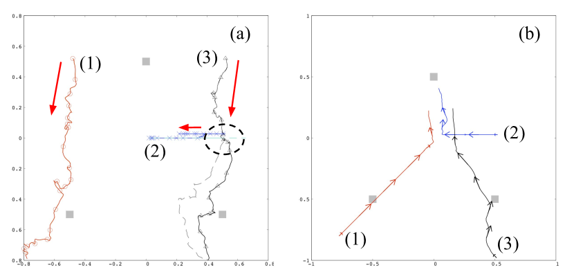
Figure 3: Agent trajectories are driven by each operation plan consequently generated via reinforcement learning [with the MLP neural network structure], $Q_{\alpha}$ first [panel (a)] and $Q_{\beta}$ [panel (b)]. The trajectories in (a) are the virtual states, ${\bm{R}}^{\left(h_{s,a}\right)}$ (two-fold), branching for Agent #2 with respect to hypothesis. Those given in (b) are the real trajectories as obtained via Eq. (17). The labels (1)-(3) indicate the agents, which move along the directions denoted by red arrows. Dotted circles indicate collisions between agents.

IV Discussions

Fig. 3(a) depicts two-fold trajectories, Eq. (14), corresponding to the hypotheses $h_{a}$ and $h_{s}$. While ${\bm{R}}^{\left(h_{a}\right)}={\bm{R}}^{\left(h_{s}\right)}$ for Agent #1, the branching ${\bm{R}}^{\left(h_{a}\right)}\neq{\bm{R}}^{\left(h_{s}\right)}$ occurs for Agent #2 during operations. The branching process earns a score via the value function $\rho^{\left(\alpha\right)}$ in Eq. (LABEL:evaluationAlpha), which indicates that the learning $Q_{\alpha}$ was conducted properly. Thus, the ability to capture the difference between $h_{a}$ and $h_{s}$ has been realized. The red dotted circle shown in (a) represents a collision between Agents #2 and #3, inducing the difference between ${\bm{R}}^{\left(h_{a}\right)}$ and ${\bm{R}}^{\left(h_{s}\right)}$ (the trajectories only reflect the central positions of agents, while each agent has a finite radius similar to its size; therefore, the trajectories themselves do not intersect even when a collision occurs). In addition, the collision strategy is never generated in a rule-based manner, as the agents autonomously deduce their strategy via reinforcement learning.

Three square symbols (closed) situated at the edges of a triangle in Fig. 3 represent the goalposts for the conveying mission. Fig. 3(b) shows the real trajectories for the mission, where the initial locations of the agents are the final locations in the panel (a). From their initial locations, Agents #1 and #3 immediately arrived at their goals to complete each mission, and subsequently headed to Agent #2 for assistance. Meanwhile, Agent #2 attempted to reach its goal using its limited mobility; i.e., only along the $x$-axis. At the closest position, all three agents Coalesced, and Agents #1 and #3 began pushing Agent #2 up toward the goal. Though this behavior is simply the consequence of earning more from the value function $\rho^{\left(\beta\right)}$, it appears as if Agent #1 wants to assist the malfunctioning agent cooperatively (a video of the behavior shown in Fig. 3(b) is available at the link Hayaschi ).? By identifying the constraint $h_{a}$ for the agents in the learning phase $Q_{\alpha}$, the subsequent learning phase $Q_{\beta}$ is confirmed to generate the optimal operation plans to ensure that the team maximizes their benefit through cooperative behavior as if an autonomous decision has been made by the team.

During training, if the target reward is not reached in the given number of training sessions, the training process is reset to avoid being trapped by the local solution. In Fig. 4, the training curves of rejected trials are shown in blue, whereas the acceptable result is shown in red. Evidently, more learning processes were rejected in $Q_{\beta}$ (right panel) than in $Q_{\alpha}$ (left panel). This indicates that it is a more challenging task to perform transport planning with three malfunctioning agents, than to plan the action to pinpoint a hypothesis among two. However, under more complex failure conditions, more learning is expected to be rejected for $Q_{\alpha}$ as well, as the number of possible hypotheses increases.

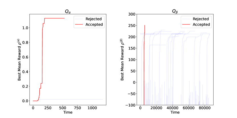
Figure 4: Learning curve evaluated for MLP network construction in terms of the reward function. Results for $Q_{\alpha}$ (left panel) and $Q_{\beta}$ (right panel) are shown. Blue and red curves correspond to trajectories that did not reach the target reward at the end of training, and those that successfully reached the target reward, respectively.

LSTM and MLP were compared in performance in terms of the success rate for obtaining working trajectories to distinguish between the hypotheses. Notably, even when applying the well-converged $Q$-table, there is a certain rate required for the non-working trajectories to eliminate the difference between the hypotheses. This is a result of the stochastic nature of the policy Eq. (6) in generating the trajectories. In the present work, we took 50 independent $Q$-tables, each of which was generated from scratch, and obtained 50 corresponding trajectories. The rate required to obtain the trajectories required to distinguish among the hypotheses amounts to 94% for LMS, and 78% for LSTM. In the present comparison, we used the same iteration steps as for $Q$-table convergence. Because LSTM has a more complex internal structure, its learning quality was expected to be relatively lower than that of LMS for the common condition, and its performance rate was likewise expected to be lower. In other words, a higher iteration cost is required for LSTM to achieve performance comparable to LMS. As such, the results shown in the main text are those obtained by LMS, whereas those obtained by LSTM are presented in the Appendix for reference.

For a simulation in a virtual environment space, we must evaluate the distances between agents at every step. As this is a pairwise evaluation, its computational cost scales as $\sim N^{2}$ for $N$ agents. This cost scaling can be mitigated by using the domain decomposition method wherein each agent is evaluated according to its voxel, and the distance between agents is represented by that between corresponding voxels registered in advance. The corresponding cost scales linearly with $N$ at a much faster rate than the naive $\sim N^{2}$ evaluation method as the number of agents $N$ increases.

V Conclusion

Agents performing group missions can suffer from errors during a missions. Multiple hypotheses may be devised to explain the causes of such errors. Cooperative behaviors, such as collisions between agents, can be deployed to identify said causes. We considered the autonomous planning of group behaviors via machine-learning techniques. Different hypothesizes explaining the causes of the errors lead to different expected states as updated from the same initial state by the same operation. The larger the difference gets, the better the corresponding operation plan is able to distinguish between the different hypotheses. In other words, the magnitude of the difference can be the value function to optimize the desired operation plan. Gradient-based optimization does not work well because a tiny fraction among the vast possible operations (e.g., collisions) can capture the difference, leading to a sparse distribution of the finite value for the function. We discovered that reinforcement learning is the obvious choice to be applied for such problems. Notably, the optimal plan obtained via reinforcement learning was the operation that causes agents to collide with each other. To identify the causes of error using this plan, we developed a revised mission plan that incorporates the failure by another learning where the malfunctioning agent receives assistance from other agents. By identifying the cause of failure, the reinforcement learning process plans a revised mission plan that considers said failure to ensure an appropriate cooperation procedure.

VI Acknowledgments

The computations in this work were performed using the facilities at Research Center for Advanced Computing Infrastructure at JAIST. R.M. is grateful for financial support from MEXT-KAKENHI (19H04692 and 16KK0097), from the Air Force Office of Scientific Research (AFOSR-AOARD/FA2386-17-1-4049;FA2386-19-1-4015). We would like to thank Kosuke Nakano for his feedback, as it significantly helped improve the overall paper.

VII Appendix

VII.1 Policy function

Getting the benefit $Q\left(\bm{R},\bm{g}\right)$, the most naive choice for the next action would be

$${\bm{g}}^{*}\left(\bm{R}\right)=\arg\max_{\bm{g}}Q\left({\bm{R}},{\bm{g}}\right)\ ,$$ (18)

known as the greedy method. This is represented in terms of the policy distribution function as

$$\pi\left(\bm{R},\bm{g}\right)=\delta\left({\bm{g}}-{\bm{g}^{*}}\left(\bm{R}\right)\right)\ .$$

To express explicitly that ${\bm{g}}^{*}\left(\bm{R}\right)$ depends on $Q\left(\bm{R},\bm{g}\right)$ via Eq. (18), let

$$\pi\left(\bm{R},\bm{g}\right)=\delta\left({\bm{g}}-{\bm{g}^{*}\left(Q\left(\bm{R},\bm{g}\right)\right)}\right)=\Delta\left(Q\left(\bm{R},\bm{g}\right)\right)\ ,$$

be a special case of

$$\pi\left(\bm{R},\bm{g}\right)=P\left(Q\left(\bm{R},\bm{g}\right)\right)\ .$$

To improve the probability of obtaining the optimal solution compared to the greedy method in a delta-function wise distribution, there are several choices allowing for a finite probability for $\bm{g}\neq\bm{g}^{*}$, including the “$\varepsilon$-greedy method“:

$$P\left(Q\left(\bm{R},\bm{g}\right)\right)=\left(1-\varepsilon\right)\cdot\Delta\left(Q\left(\bm{R},\bm{g}\right)\right)+\varepsilon\cdot\left[{\rm RandomNubmer}\right]\ ,$$

and the “Boltzmann policy“:

$$P\left(Q\left(\bm{R},\bm{g}\right)\right)=\exp\left(-\beta Q\left(\bm{R},\bm{g}\right)\right)\ .$$

VII.2 Results using LSTM

As explained in the main text, reinforcement learning using the LSTM neural network structure leads to nearly identical behaviors for the agents, though it requires a lower rate to obtain working trajectories to distinguish among the hypotheses. Figs. 5 and  6 show the optimized trajectories and learning curves, respectively (counterparts of Figs. 3 and  4, respectively).

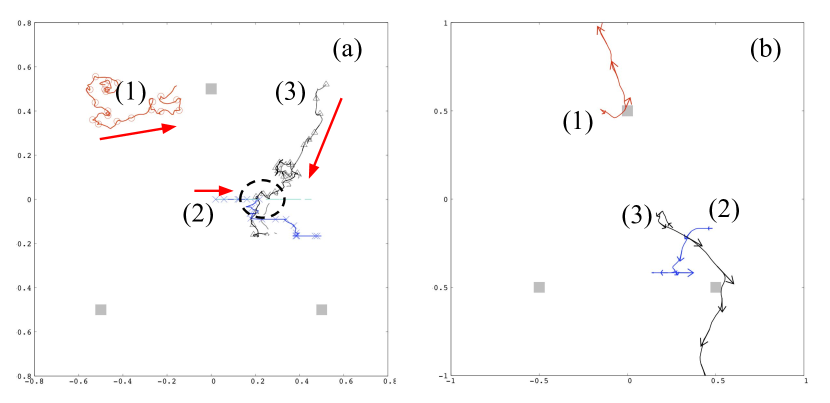
Figure 5: Agent trajectories driven by each operation plan generated via reinforcement learning [with LSTM], $Q_{\alpha}$ first [panel (a)] and $Q_{\beta}$ [panel (b)], consequently. The trajectories in (a) are the virtual states, ${\bm{R}}^{\left(h_{s,a}\right)}$ (two-fold), branching for Agent #2 with respect to each hypothesis. Those given in (b) are the real trajectories as given in Eq. (17). The labels (1)-(3) represent agents, which move along the directions denoted by red arrows. Dotted circles indicate collisions between agents.

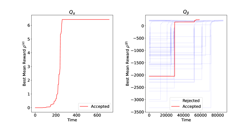
Figure 6: Learning curve in terms of the reward function, evaluated for LSTM network construction. Results for $Q_{\alpha}$ (left panel) and $Q_{\beta}$ (right panel) are shown. Blue and red curves correspond to trajectories that did not reach the target reward at the end of training, and those that successfully reached the target reward, respectively.

References

- Lee et al. (2018) H. Lee, H. Kim, and H. J. Kim, IEEE Transactions on Automation Science and Engineering 15, 189 (2018).
- Hu et al. (2020) J. Hu, H. Niu, J. Carrasco, B. Lennox, and F. Arvin, IEEE Transactions on Vehicular Technology 69, 14413 (2020).
- Friston (2010) K. Friston, Nature Reviews Neuroscience 11, 127 (2010).
- Huang et al. (2005) B.-Q. Huang, G.-Y. Cao, and M. Guo, in 2005 International Conference on Machine Learning and Cybernetics, Vol. 1 (2005) pp. 85–89.
- Xia and El Kamel (2016) C. Xia and A. El Kamel, Robotics and Autonomous Systems 84, 1 (2016).
- Zhu et al. (2018) D. Zhu, T. Li, D. Ho, C. Wang, and M. Q.-H. Meng, in 2018 IEEE International Conference on Robotics and Automation (ICRA) (2018) pp. 7548–7555.
- Nachum et al. (2018) O. Nachum, S. Gu, H. Lee, and S. Levine, in Proceedings of the 32nd International Conference on Neural Information Processing Systems (2018) pp. 3307–3317.
- Sutton and Barto (2018) R. S. Sutton and A. G. Barto, Reinforcement Learning: An Introduction, 2nd ed. (The MIT Press, 2018).
- Barto (2002) A. G. Barto, in The Handbook of Brain Theory and Neural Networks, Second Edition, edited by M. A. Arbib (The MIT Press, Cambridge, MA, 2002) pp. 963–972.
- Peng et al. (2018) X. B. Peng, M. Andrychowicz, W. Zaremba, and P. Abbeel, in 2018 IEEE International Conference on Robotics and Automation (ICRA) (2018) pp. 3803–3810.
- Finn and Levine (2017) C. Finn and S. Levine, in 2017 IEEE International Conference on Robotics and Automation (ICRA) (2017) pp. 2786–2793.
- Mnih et al. (2015) V. Mnih, K. Kavukcuoglu, D. Silver, A. A. Rusu, J. Veness, M. G. Bellemare, A. Graves, M. Riedmiller, A. K. Fidjeland, G. Ostrovski, S. Petersen, C. Beattie, A. Sadik, I. Antonoglou, H. King, D. Kumaran, D. Wierstra, S. Legg, and D. Hassabis, Nature 518, 529 (2015).
- Silver et al. (2017) D. Silver, J. Schrittwieser, K. Simonyan, I. Antonoglou, A. Huang, A. Guez, T. Hubert, L. Baker, M. Lai, A. Bolton, Y. Chen, T. Lillicrap, F. Hui, L. Sifre, G. van den Driessche, T. Graepel, and D. Hassabis, Nature 550, 354 (2017).
- Vinyals et al. (2019) O. Vinyals, I. Babuschkin, W. M. Czarnecki, M. Mathieu, A. Dudzik, J. Chung, D. H. Choi, R. Powell, T. Ewalds, P. Georgiev, J. Oh, D. Horgan, M. Kroiss, I. Danihelka, A. Huang, L. Sifre, T. Cai, J. P. Agapiou, M. Jaderberg, A. S. Vezhnevets, R. Leblond, T. Pohlen, V. Dalibard, D. Budden, Y. Sulsky, J. Molloy, T. L. Paine, C. Gulcehre, Z. Wang, T. Pfaff, Y. Wu, R. Ring, D. Yogatama, D. Wünsch, K. McKinney, O. Smith, T. Schaul, T. Lillicrap, K. Kavukcuoglu, D. Hassabis, C. Apps, and D. Silver, Nature 575, 350 (2019).
- Busoniu et al. (2006) L. Busoniu, R. Babuska, and B. De Schutter, in 2006 9th International Conference on Control, Automation, Robotics and Vision (2006) pp. 1–6.
- Gupta et al. (2017) J. K. Gupta, M. Egorov, and M. Kochenderfer, in Autonomous Agents and Multiagent Systems, edited by G. Sukthankar and J. A. Rodriguez-Aguilar (Springer International Publishing, Cham, 2017) pp. 66–83.
- Straub et al. (2020) K. M. Straub, B. Bontempo, F. Jones, A. M. Jones, P. Farr, and T. Bihl, ensor Resource Management using Multi-Agent Reinforcement Learning with Hyperparameter Optimization, Tech. Rep. (2020) white paper.
- Bihl et al. (2020a) T. Bihl, P. Farr, K. M. Straub, B. Bontempo, and F. Jones, in Hawaii International Conference on Systems Sciences 2022 (2020) submitted.
- Gronauer and Diepold (2021) S. Gronauer and K. Diepold, Artificial Intelligence Review (2021), 10.1007/s10462-021-09996-w.
- Malhotra et al. (2017) R. P. Malhotra, M. J. Pribilski, P. A. Toole, and C. Agate, in Micro- and Nanotechnology Sensors, Systems, and Applications IX, Vol. 10194, edited by T. George, A. K. Dutta, and M. S. Islam, International Society for Optics and Photonics (SPIE, 2017) pp. 403 – 414.
- Malhotra et al. (1997) R. Malhotra, E. Blasch, and J. Johnson, in Proceedings of the IEEE 1997 National Aerospace and Electronics Conference. NAECON 1997, Vol. 2 (1997) pp. 769–776 vol.2.
- Hero and Cochran (2011) A. O. Hero and D. Cochran, IEEE Sensors Journal 11, 3064 (2011).
- Nguyen et al. (2020) T. T. Nguyen, N. D. Nguyen, and S. Nahavandi, IEEE Transactions on Cybernetics 50, 3826 (2020).
- Foerster et al. (2017) J. Foerster, N. Nardelli, G. Farquhar, T. Afouras, P. H. S. Torr, P. Kohli, and S. Whiteson, in Proceedings of the 34th International Conference on Machine Learning, Proceedings of Machine Learning Research, Vol. 70, edited by D. Precup and Y. W. Teh (PMLR, 2017) pp. 1146–1155.
- Calvo and Dusparic (2018) J. Calvo and I. Dusparic, in Proc. 26th Irish Conf. Artif. Intell. Cogn. Sci. (2018) pp. 1–12.
- Wang and Taylor (2017) Z. Wang and M. E. Taylor, in Proceedings of the Twenty-Sixth International Joint Conference on Artificial Intelligence, IJCAI-17 (2017) pp. 3027–3033.
- Brockman et al. (2016) G. Brockman, V. Cheung, L. Pettersson, J. Schneider, J. Schulman, J. Tang, and W. Zaremba, “Openai gym,” (2016), arXiv:1606.01540 .
- Schulman et al. (2015) J. Schulman, S. Levine, P. Mortiz, M. Jordan, and P. Abbeel, in Proceedings of the 32nd International Conference on Machine Learning - Volume 37 (2015) pp. 1889–1897.
- Henderson et al. (2018) P. Henderson, R. Islam, P. Bachman, J. Pineau, D. Precup, and D. Meger, in AAAI (2018).
- Bihl et al. (2020b) T. J. Bihl, J. Schoenbeck, D. Steeneck, and J. Jordan, in 53rd Hawaii International Conference on System Sciences, HICSS 2020, Maui, Hawaii, USA, January 7-10, 2020 (ScholarSpace, 2020) pp. 1–10.
- Snoek et al. (2012) J. Snoek, H. Larochelle, and R. P. Adams, in Proceedings of the 25th International Conference on Neural Information Processing Systems - Volume 2 (2012) pp. 2951–2959.
- Domhan et al. (2015) T. Domhan, J. T. Springenberg, and F. Hutter, in Proceedings of the 24th International Conference on Artificial Intelligence (2015) pp. 3460–3468.
- Young et al. (2020) M. T. Young, J. D. Hinkle, R. Kannan, and A. Ramanathan, Journal of Parallel and Distributed Computing 139, 43 (2020).
- (34) K. Hayaschi, “Video for fig. 3. (b),” https://www.dropbox.com/s/feejhj389h7p215/robot2_labeled.mp4?dl=0.