Abstract

Increasingly complex data analysis tasks motivate the study of the dependency of distributions of multivariate continuous random variables on scalar or vector predictors. Statistical regression models for distributional responses so far have primarily been investigated for the case of one-dimensional response distributions. We investigate here the case of multivariate response distributions while adopting the 2-Wasserstein metric in the distribution space. The challenge is that unlike the situation in the univariate case, the optimal transports that correspond to geodesics in the space of distributions with the 2-Wasserstein metric do not have an explicit representation for multivariate distributions. We show that under some regularity assumptions the conditional Wasserstein barycenters constructed for a geodesic in the Euclidean predictor space form a corresponding geodesic in the Wasserstein distribution space and demonstrate how the notion of conditional barycenters can be harnessed to interpolate as well as extrapolate multivariate distributions. The utility of distributional inter- and extrapolation is explored in simulations and examples. We study both global parametric-like and local smoothing-like models to implement conditional Wasserstein barycenters and establish asymptotic convergence properties for the corresponding estimates. For algorithmic implementation we make use of a Sinkhorn entropy-penalized algorithm. Conditional Wasserstein barycenters and distribution extrapolation are illustrated with applications in climate science and studies of aging.

KEY WORDS: Optimal Transport, Fréchet Mean, Wasserstein Metric, Geodesics, Sinkhorn Penalty, Climate Change, Baltimore Longitudinal Study of Aging.

1 Introduction

Optimal transport and the associated Wasserstein distance, also known as earth mover’s distance (Rubner et al., 2000), have been widely used in analyzing probability distributions and their relationships (Villani, 2008). Especially the Wasserstein barycenter problem (Agueh and Carlier, 2011) has met with growing interest in many fields including machine learning (Genevay et al., 2018; Frogner et al., 2015; Rabin et al., 2011), physics (Buttazzo et al., 2012) and economics (Carlier and Ekeland, 2010). The $p$-Wasserstein metric in the space of distributions is motivated by the Monge–-Kantorovich transportation problem, where the Kantorovich version of the problem (Villani, 2008) is

$$W_{p}^{p}(\mu,\nu)=\inf_{\mathbf{\mu}\in\Pi(\mu,\nu)}E_{(X,Y)\sim\mathbf{\mu}}\|X-Y\|^{p}.$$

Here $X,Y$ are random variables in $\mathbb{R}^{d}$, $\mu,\nu$ are probability measure supported on a set $M\subset\mathbb{R}^{d}$, and $\Pi(\mu,\nu)$ is the space of joint probability measures on $M\times M$ with marginals $\mu$ and $\nu$. There is a close connection to Monge’s transport problem (Monge, 1781), where optimal transport is characterized by

$$OT^{p}(\mu,\nu)=\inf_{T:T_{\#}\mu=\nu}E_{X\sim\mu}\|X-T(X)\|^{p}$$

and the optimization is taken over all push-forward maps $T$ that map $\mu$ to $\nu$. The push-forward maps $T$ are Borel maps $M\rightarrow M$ and with $\nu_{1}$ denoting any probability measure on $M$, $\nu_{2}=T_{\#}\nu_{1}$ stands for the push-forward measure of $\nu_{1}$, defined as the measure satisfying $\nu_{2}(M_{1})=\nu_{1}(T^{-1}(M_{1}))$ for any measurable set $M_{1}\subset M$. If it exists, the minimizer $\operatorname*{arg\,inf}_{T:M\rightarrow M}E_{X\sim\mu}\|X-T(X)\|^{p}$ is the optimal transport plan. In general, the Kanorovich and Monge problems do not admit the same solution. But when Monge’s problem has a minimizer $T_{0}$, it is also a solution of Kantorovich’s problem. If $\mu$ is absolutely continuous, the two problems are equivalent (Villani, 2008) .

For the special case of distributions on the real line $R^{1}$, the $p$-Wasserstein distance between probability distributions is well known to correspond to the $L^{p}$ distance between their quantile functions. If $F_{\mu_{1}},F_{\mu_{2}}$ denote the cumulative distribution functions of measures $\mu_{1}$ and $\mu_{2}$, the $p$-Wasserstein distance can be written as

$$W_{p}^{p}(\mu_{1},\mu_{2})=\int_{0}^{1}(F_{\mu_{1}}^{-1}(s)-F_{\mu_{2}}^{-1}(s))^{p}ds,$$ (1)

where $F_{1}^{-1},F_{2}^{-1}$ are left inverses of $F_{1},F_{2}$. The most commonly used Wasserstein distances are the 1-Wasserstein and 2-Wasserstein distances, not least since their geodesics are easily interpretable. A comparative example of geodesics in the 2-Wasserstein space and in the space of distributions with the $L^{2}$ distance between densities is provided in Figure 1 for the case of two-dimensional Gaussian densities , where it is seen that the 2-Wasserstein geodesics are more intuitive and better interpretable than the $L^{2}$ geodesics. Accordingly, we focus here on 2-Wasserstein barycenters for distributions in the finite-dimensional Euclidean space $R^{d}$ and consider their extension to conditional barycenters.

For a random measure $\nu$ taking values in 2-Wasserstein space $\mathcal{W}_{2}$, the 2-Wasserstein barycenter of $\nu$ is defined as (Le Gouic and Loubes, 2017)

$$B(\nu)=\operatorname*{arg\,inf}_{\mu\in\mathcal{W}_{2}}EW^{2}_{2}(\mu,\nu).$$ (2)

Similarly, when a sample of measures $\{\nu_{i}\}$, $i=1,2,\ldots,n$ is observed, the sample 2-Wasserstein barycenter (Agueh and Carlier, 2011) is

$$B(\nu_{1},\ldots,\nu_{n})=\operatorname*{arg\,inf}_{\mu\in\mathcal{W}_{2}}\sum_{i=1}^{n}W_{2}^{2}(\nu_{i},\mu).$$

For $n$ nonnegative weights with $w_{i}>0,\,\sum_{i=1}^{n}w_{i}=1$, a weighted version of the 2-Wasserstein sample barycenter is analogoulsy defined as

$$B_{(w_{1},\ldots,w_{n})}(\nu_{1},\ldots,\nu_{n})=\operatorname*{arg\,inf}_{\mu\in\mathcal{W}_{2}}\sum_{i=1}^{n}w_{i}W_{2}^{2}(\nu_{i},\mu).$$ (3)

Sample or empirical barycenters can also be viewed as sample Fréchet means (Fréchet, 1948) of $\{\nu_{i}\}$ in the Wasserstein space. Existence and uniqueness of 2-Wasserstein barycenters has been shown under the assumption of absolute continuity of the measures $\nu_{i}$, where Le Gouic and Loubes (2017) also studied the convergence of sample barycenters towards the population barycenter. While the properties of empirical barycenters and their computation have been well studied, the situation is quite different for conditional barycenters. From a statistical perspective, the conditional barycenter problem was addressed in Petersen and Müller (2019) for the special setting of probability measures on $R^{1}$ as responses. In the one-dimensional case one can alternatively pursue global transformations that map the Wasserstein space of one-dimensional distributions to a Hilbert space $L^{2}$ (Petersen and Müller, 2016) or alternatively of log maps to tangent bundles in the Wasserstein manifold (Bigot et al., 2017, 2018; Chen et al., 2020), although both come at the price of a metric distortion. After applying such a transformation, functional regression models designed for linear spaces naturally become applicable in the ensuing Hilbert spaces (Horvath and Kokoszka, 2012; Wang et al., 2016).

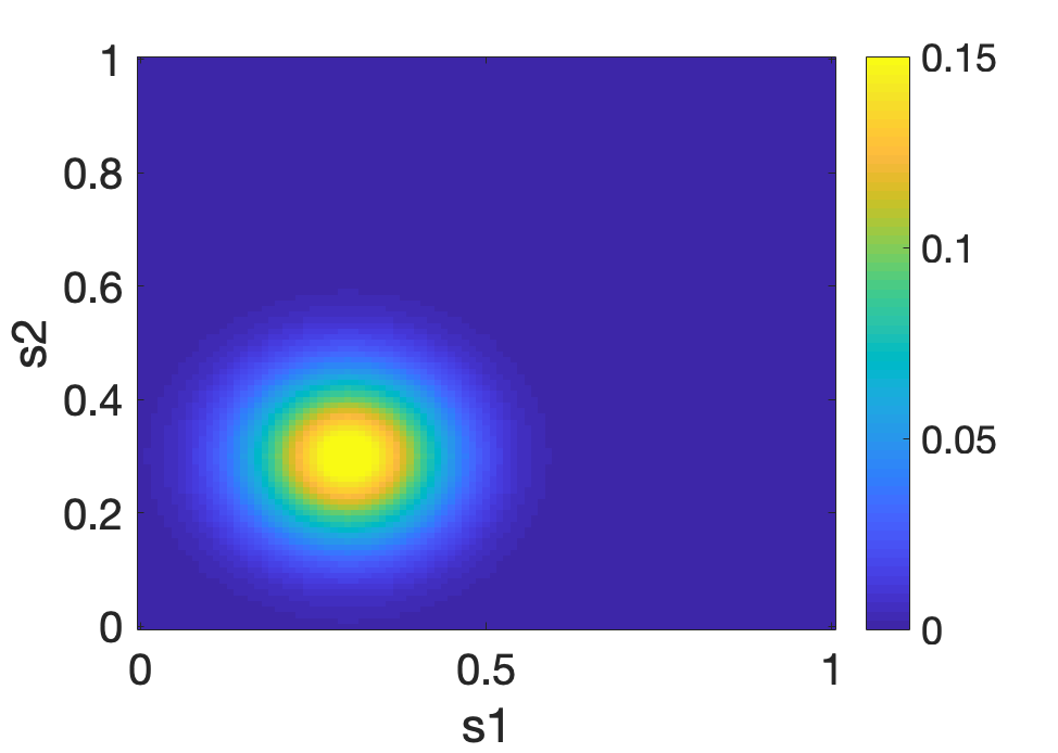
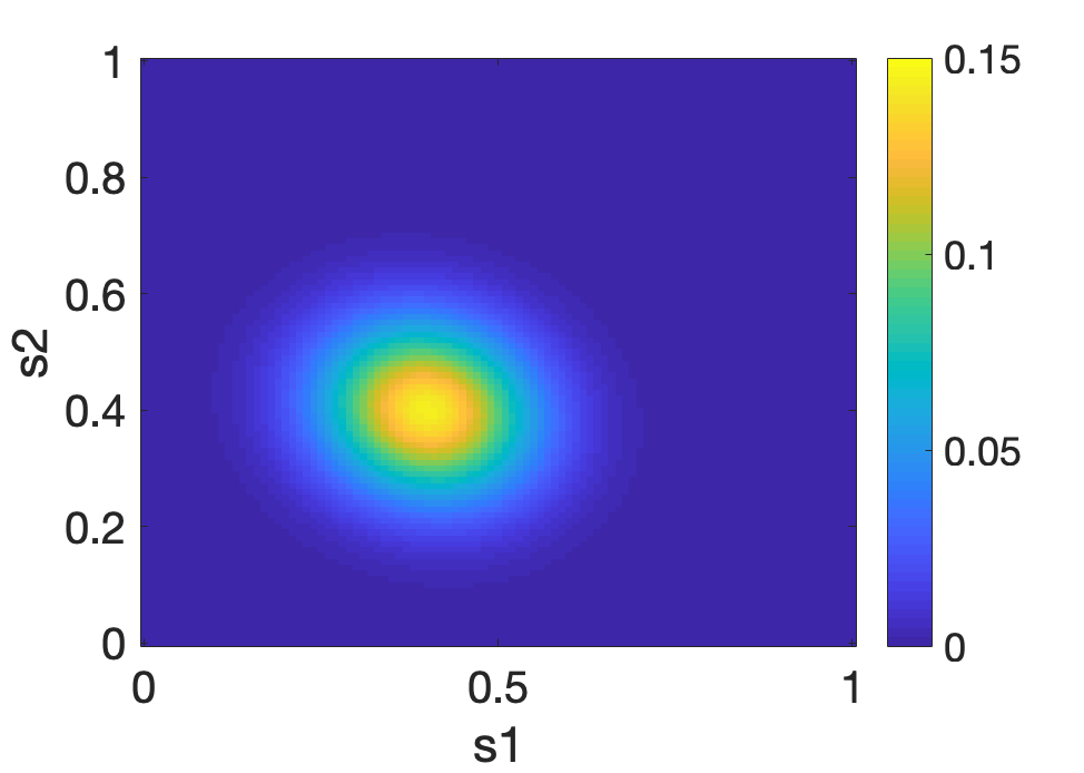
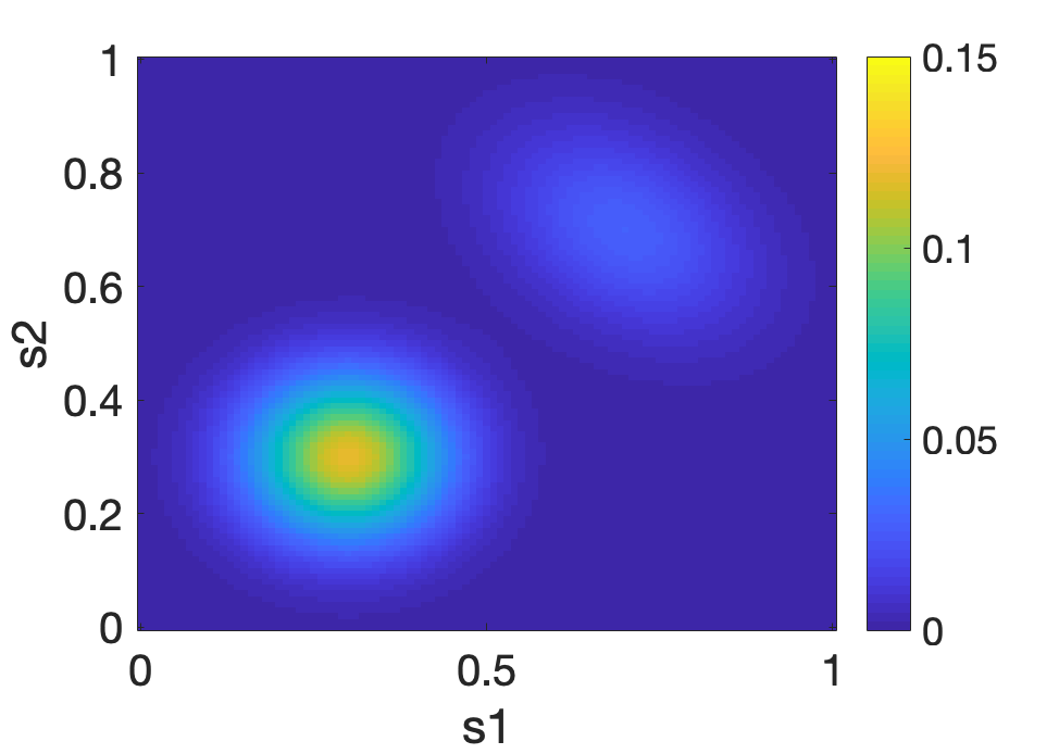
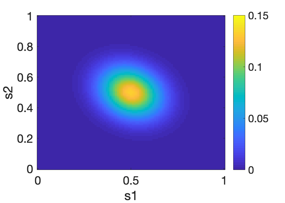
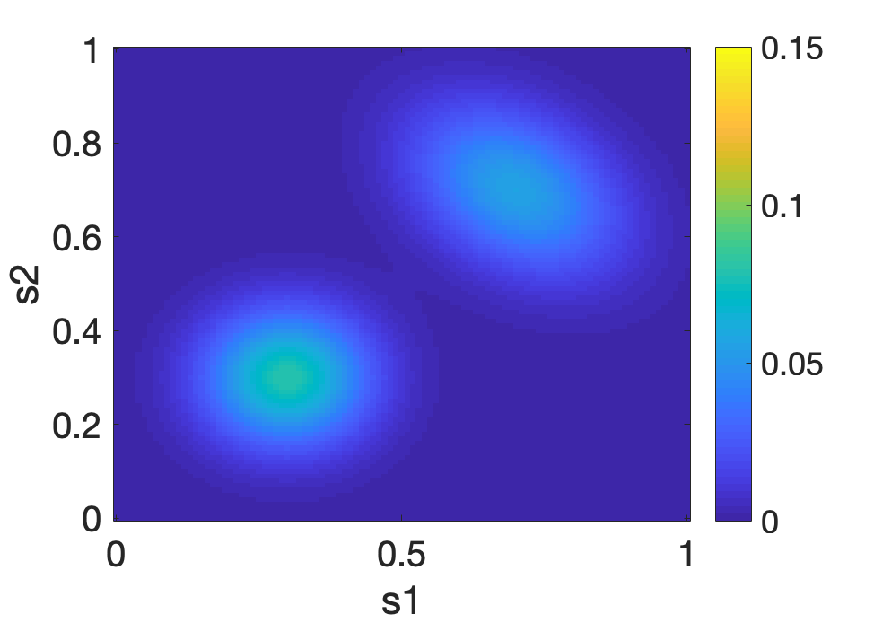
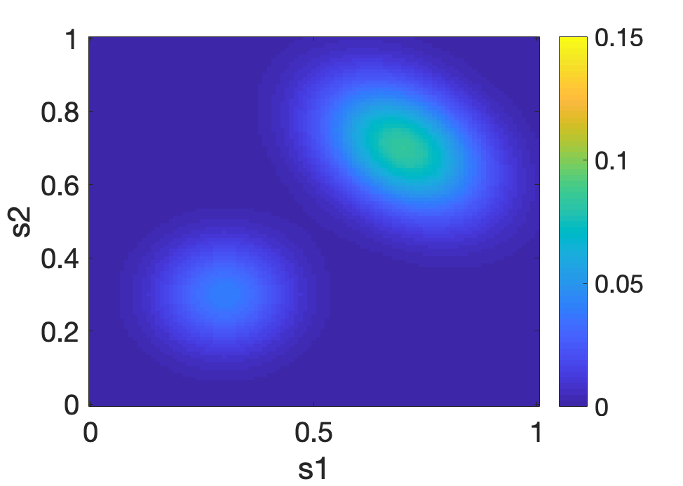
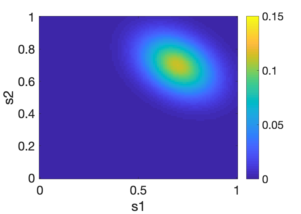
Figure 1: Wasserstein (left panel) and $L^{2}$ (right panel) geodesics at levels $x=0,0.25,0.5,0.75,1$, from top to bottom, interpolating the Gaussian distributions $N((4,4),[1\,0;0\,1])$ (for $x=0$) and $N((6,6),[1.25\,-0.25;-0.25\,1.25])$ (for $x=1$) and illustrated as heat maps of the respective distributions.

In this paper we aim to address the problem of estimating conditional barycenters in general $R^{d}$ spaces, where such transformations are not known or face major difficulties in theory and implementation so that the barycenter problem cannot be linearized in this way. Then the notion of conditional barycenters replaces the traditional conditional expectation and forms the backbone for the proposed regression models with responses that are distributions in $\mathbb{R}^{p}$ and are coupled with Euclidean predictors. The paper is organized as follows. Section 2 introduces the problem of conditional barycenters and the statistical models that are proposed for their implementation. Algorithmic aspects for obtaining the conditional Wasserstein barycenter in $R$ and $R^{d}$, $d\geq 2$ respectively, are discussed in section 3. Section 4 contains a study of the asymptotic behavior of corresponding estimates of the conditional barycenters. In Sections 5 and 6, we provide simulation results and data analysis to illustrate the methodology and provide additional motivation. All proofs are in the Supplement.

2 Global and Local Models for Conditional Barycenters

In standard regression modeling in Euclidean spaces, one postulates an explicit model for the conditional expectation $E(Y|X)$ for responses $Y$, given predictors $X$, to quantify their relationship. A classical model is $E(Y|X)=\beta X$ for global linear models with a parameter vector $\beta$. The utility of such a model is often not more than providing a useful approximation (Buja et al., 2019a, b). Simplified and often approximative regression models are necessary as the direct modeling of the joint distribution of $(X,Y)$, from which the actual regression relation derives, usually proves too complex for statistical modeling. It is possible in some cases to relax the assumption of global linearity and to adopt less restrictive local linear models that adapt better to nonlinear shapes. The situation becomes more complex when non-Euclidean data such as elements of the Wasserstein space are involved in the joint distribution. In the situation we consider here, responses $Y$ are distributions and one then needs an appropriate definition of the conditional barycenter, and, importantly, of the specific regression model through which it can be implemented.

Consider random objects $(X,\nu)$ with $\nu$ taking values in the 2-Wasserstein space $\mathcal{W}_{2}(M)$ of probability measures supported on a compact domain $M\in R^{d}$, where $X\in R^{q},\,\text{ with }d,q\geq 1.$ More specifically, to exclude complications that arise when dealing with discrete measures and are of no interest for our purposes, we restrict the probability measures $\nu$ to the subset of absolutely continuous measures so that each measure is associated with a unique density $f_{\nu}$ and denote this subset of probability measures as $\Omega=\mathcal{W}_{2}(M)\cap\mathcal{C}(M)$, $\mathcal{C}(M)$ denoting the set of absolutely continuous measures on $M$. Since the density space equipped with the Wasserstein metric is not a Hilbert space, the usual notion of expectation is not sensible and is replaced by the Fréchet mean (Fréchet, 1948), which is the barycenter given in (2), with $\mathcal{W}_{2}$ replaced by $\Omega$. The concept of conditional barycenters was introduced in Petersen and Müller (2019) for metric space-valued responses and shown to apply to one-dimensional distributions. Its general definition for probability distributions on spaces $R^{d}$ or on more general metric spaces is

Definition 1.

(Conditional Wasserstein Barycenter). Assume $(X,\nu)$ has a joint distribution. The conditional Wasserstein barycenter is defined as the Fréchet regression, or conditional Fréchet mean with respect to the 2-Wasserstein distance, i.e.,

$$\mu_{0}(x)=\operatorname*{arg\,min}_{\mu\in\Omega}E(W_{2}^{2}(\mu,\nu)|X=x).$$ (4)

To implement this general concept, one needs specific models for these conditional barycenters, in the same way as one needs specific regression models to implement conditional expectations for Euclidean data, such as $E(Y|X)=\beta X$ for a global linear model or $E(Y|X)=m(X)$ with a twice differential function $m$ for a local linear model. Specifically, we aim to obtain conditional Wasserstein barycenters from samples $\{X_{i},f_{i}\},\,i=1,2,\ldots,n$, where the $f_{i}$ are densities supported on $M$. Here we use densities to represent probability measures in $\Omega$, as they are assumed to be well defined and are easier to interpret statistically compared to other equivalent representations.

It has remained an open question whether the Fréchet regression approach can be applied to multivariate distributions. Fréchet regression provides versions of a global (linear) model and a local (linear) model, designed for metric space valued random objects satisfying certain regularity conditions that were shown to be met for one-dimensional distributions (Petersen and Müller, 2019). The technical difficulties one faces for the case of multivariate distributions differ fundamentally from the situation for one-dimensional distributions, as it is not possible anymore to take advantage of $L^{2}$ vector space operations in the space of quantile functions as per (1), which is a crucial element of the previous analysis.

In this paper we show that under certain assumptions the extension of global and local linear models for conditional barycenters to the much larger class of multivariate distributions is feasible, and study the convergence of corresponding estimates to the population targets. Relevant applications include extrapolating multivariate distributions beyond the range of the predictor $X$ similar to linear extrapolation in the Euclidean case, in addition to interpolation. Consistency of estimates for the global model is attained if the conditional barycenters have a specific form, while the local model more broadly approximates the true conditional barycenters under mild assumptions and works well for low-dimensional predictors $X$. The local model is especially useful to interpolate conditional barycenters for continuous predictors that may be observed on a discrete grid while one desires conditional barycenters for all predictor values without postulating a global linear model.

Let $\nu_{i}$ be random probability measures with density $f_{i},\,i=1,\dots,n,$ where we write $\nu$ and $f$ for generic measures and densities. The global model for conditional Wasserstein barycenter is defined as

$$\mu_{G}(x)=\operatorname*{arg\,min}_{\mu\in\Omega}E(s_{G}(X,x)W_{2}^{2}(\mu,\nu)),$$ (5)

where $s_{G}(X,x)=1+(X-E(X))^{t}{\rm Var}(X)^{-1}(x-E(X))$ is a weight function that is linear in $x$. With $\mathcal{\lambda}$ denoting the Lebesgue measure on $M$, the density corresponding to $\mu_{G}(x)$ is $f_{G}(x,\cdot)=\frac{d\mu_{G}(X)}{d\lambda}$. The corresponding sample version for the global conditional Wasserstein barycenter estimate is

$$\hat{\mu}_{G}(x)=\operatorname*{arg\,min}_{\mu\in\Omega}\frac{1}{n}\sum_{i=1}^{n}s_{iG}(x)W_{2}^{2}(\mu,\nu_{i}),$$ (6)

where $s_{iG}(x)=1+(X_{i}-\bar{X})^{t}\Sigma^{-1}(x-\bar{X})$ is the empirical version of $s_{G}(X,x)$. The corresponding density is $\hat{f}_{G}(x,\cdot)=\frac{d\hat{\mu}_{G}(X)}{d\lambda}$. These notions are analogous to the extension of the usual mean to the Fréchet mean, namely, they are extensions of the characterization of a linear regression with scalar response, which is found to minimize (5) and (6) for the Euclidean metric, to the case of general metric space valued responses; additional motivation and connections to M estimation can be found in Petersen and Müller (2019).

For a kernel function $K$ on $M$ which is a probability density and a vector of positive bandwidths $h\in R^{d}$, the local model for conditional Wasserstein barycenters is

$$\mu_{L,h}(x)=\operatorname*{arg\,min}_{\mu\in\Omega}E(s_{L,h}(X,x)W_{2}^{2}(\mu,\nu)),$$ (7)

where $s_{L,h}(X,x)=\frac{1}{\sigma_{0}^{2}}K_{h}(X-x)[1-\mu_{1}^{t}\mu_{2}^{-1}(X-x)]$, $\sigma_{0}^{2}=\mu_{0}-\mu_{1}^{t}\mu_{2}^{-1}\mu_{1}$, $\mu_{0}=E(K_{h}(X-x)),\,\mu_{1}=E(K_{h}(X-x)(X-x)),\,\mu_{2}=E(K_{h}(X-x)(X-x)(X-x)^{t})$, and the corresponding density is $f_{L,h}(x,\cdot)=\frac{d\mu_{L,h}(x)}{d\lambda}$.

The motivation again is the extension of means to Fréchet means and rewriting the local linear estimates as M-estimators. The corresponding sample version is

$$\hat{\mu}_{L,h}(x)=\operatorname*{arg\,min}_{\mu\in\Omega}\frac{1}{n}\sum_{i=1}^{n}s_{iL,h}(x)W_{2}^{2}(\mu,\nu),$$ (8)

where $s_{iL,h}(x)=\frac{1}{\hat{\sigma}_{0}^{2}}K_{h}(X_{i}-x)(1-\hat{\mu}_{1}^{t}\hat{\mu}_{2}^{-1}(X_{i}-x))$, $\hat{\sigma}_{0}^{2}=\hat{\mu}_{0}-\hat{\mu}_{1}^{t}\hat{\mu}_{2}^{-1}\hat{\mu}_{1}$ and $\hat{\mu}_{j}=\frac{1}{n}\sum_{i=1}^{n}K_{h}(X_{i}-x)(X_{i}-x)^{j}$, with corresponding density $\hat{f}_{L,h}(x,\cdot)=\frac{d\hat{\mu}_{L,h}(x)}{d\lambda}$. We note that the weights used in (7) and (8) are not constrained to be positive and indeed some of the weights are usually negative, especially when the predictors are near a boundary of the predictor domain. It is straightforward to see, for example in the Euclidean case, that negative weights are an inherent necessity and are indeed required to represent global and local linear regression relations.

While these global and local models to implement conditional barycenters can be viewed as instantiations of the general Fréchet regression paradigm, our focus here is to study the features of the population versions and the properties of the resulting estimates in the multivariate distribution case. For this important case the properties of these models have remained unknown so far and implementations also involve non-trivial computational aspects that will be explored in the following section.

3 Computational Considerations

When the dimension $d$ of the random probability measures that we study here is more than 1, i.e., $d\geq 2$, one does not have an analytic form for the barycenter and the optimization algorithms to obtain it are complex, in contrast to the case $d=1$, where the quantile representation of Wasserstein distance as per (1) leads to an explicit solution via the $L^{2}$ mean of the quantile functions. The computation of Wasserstein barycenters in multidimensional Euclidean space has been intensively studied (e.g., Rabin et al., 2011; Álvarez-Esteban et al., 2016; Dvurechenskii et al., 2018; Peyré and Cuturi, 2019), and one of the most popular methods utilizes the Sinkhorn divergence (Cuturi, 2013), which is an entropy-regularized version of the Wasserstein distance that allows for computationally efficient solutions of the barycenter problem, however at the cost of introducing a bias, as is common for regularized estimation. Due to the gain in efficiency, we adopt this approach in our implementations.

For the straightforward case $d=1$, where the Wasserstein distance is the $L^{2}$ distance of the quantile functions $W_{2}^{2}(\mu_{1},\mu_{2})=\int_{0}^{1}(F_{\mu_{1}}^{-1}(t)-F_{\mu_{2}}^{-1}(t))^{2}dt,$ the following result has been established previously, which greatly facilitates the study of conditional barycenters for this case.

Proposition 1 (Global and local estimates for $d=1$ (Petersen and Müller, 2019)).

For one-dimensional probability measures $\mu_{i},\,i=1,2,\ldots,n$, denoting by $\mathcal{Q}$ the space of quantile functions, the solutions of the global and local Wasserstein barycenter problems (6) and (8) are obtained as the distributions with the following quantile functions,

$$F_{\hat{\mu}_{G}(x)}^{-1}(\cdot)=\operatorname*{arg\,min}_{Q\in\mathcal{Q}}\|Q-\frac{1}{n}\sum_{i=1}^{n}s_{iG}(x)F_{\mu_{i}}^{-1}(\cdot)\|^{2}_{2}$$

$$F_{\hat{\mu}_{L,h}(x)}^{-1}(\cdot)=\operatorname*{arg\,min}_{Q\in\mathcal{Q}}\|Q-\frac{1}{n}\sum_{i=1}^{n}s_{iL,h}(x)F_{\mu_{i}}^{-1}(\cdot)\|^{2}_{2}.$$

For the case $d>1$, the distribution is often only observed on a discrete grid, an assumption that is almost universally made for computational implementations. Accordingly, we consider an equidistant rectangular grid $(d_{1},\ldots,d_{m})$ on the domain $M\subset R^{d}$. Since $M$ is assumed to be compact, there exists a rectangle $\tilde{M}$ such that $M\subset\tilde{M}$. The grid $(d_{1},\ldots,d_{m})$ is constructed by first creating an equidistant rectangular grid $(d_{1},\ldots,d_{\tilde{m}})$ on $\tilde{M}$ and then $\{d_{1},\ldots,d_{m}\}=\{d_{1},\ldots,d_{\tilde{m}}\}\cap M$, then representing the observed densities $f_{i}(x)$ as length $m$ vectors $(f_{i}(d_{1}),f_{i}(d_{2}),\ldots,f_{i}(d_{m}))$. Prior to computing the Wasserstein distance, the densities are approximated by the discrete measure vector $\mathbf{r}_{i}=(\frac{f_{i}(d_{1})}{\sum_{j=1}^{m}f_{i}(d_{i})},\frac{f_{i}(d_{2})}{\sum_{j=1}^{m}f_{i}(d_{i})},\ldots,\frac{f_{i}(d_{m})}{\sum_{j=1}^{m}f_{i}(d_{i})})$.

The following result quantifies the approximation error in terms of the Wasserstein distance between a continuous measure $\nu$ and its discrete approximation $\nu_{r}$.

Proposition 2 (Approximation of a continuous measure with a discrete measure).

Consider an absolutely continuous probability measure $\nu$ on $M$ with density $f_{\nu}$ and an equidistant rectangular grid $(d_{1},...,d_{m})$ with probability mass $\mathbf{r}$ as described above. If the density $f_{\nu}$ is Lipschitz continuous, then

$$W^{2}_{2}(\nu,\nu_{\mathbf{r}})=O(\min_{k,l,k\neq l}\|d_{k}-d_{l}\|^{2})$$

as $\min_{k,l,k\neq l}\|d_{k}-d_{l}\|^{2}\rightarrow 0$.

Denoting the pairwise distance matrix of the grid by $D=(\|d_{k}-d_{l}\|^{2})_{k,l}$, the 2-Wasserstein distance can be written as

$$W_{2}^{2}(\mathbf{r}_{i},\mathbf{r}_{j})=\min_{S\in U(\mathbf{r}_{i},\mathbf{r}_{j})}\langle S,D\rangle,$$ (9)

where $U(\mathbf{r}_{i},\mathbf{r}_{j})=\{S\in R_{\oplus}^{m\times m}|S\mathbf{1}_{m}=\mathbf{r}_{i},\,S^{\prime}\mathbf{1}_{m}=\mathbf{r}_{j}\}$. Then the conditional Wasserstein barycenter estimates become

$$\hat{\mathbf{r}}_{G}(x)=\operatorname*{arg\,min}_{\mathbf{r}\in\mathcal{D}}\sum_{i=1}^{n}s_{iG}(x)\min_{S_{i}\in U(\mathbf{r},\mathbf{r}_{i})}\langle S_{i},D\rangle$$

$$\hat{\mathbf{r}}_{L,h}(x)=\operatorname*{arg\,min}_{\mathbf{r}\in\mathcal{D}}\sum_{i=1}^{n}s_{iL,h}(x)\min_{S_{i}\in U(\mathbf{r},\mathbf{r}_{i})}\langle S_{i},D\rangle,$$

where $\mathcal{D}=\{(r_{1},r_{2},\cdots,r_{m})|r_{k}\geq 0,\,\sum_{j=1}^{m}r_{k}=1\}$. This problem can typically be solved by linear programming (Anderes et al., 2016). However, with a grid of large size, e.g. $100\times 100$ in $R^{2}$ this may not be satisfactory, as linear programming does not scale well and has a computational complexity of the order $O(nm^{3}\log m)$.

To address this problem, we adopt Sinkhorn divergence, a regularized version of Wasserstein distance, (Cuturi, 2013). Various approaches have been developed to compute Sinkhorn barycenters (e.g., Cuturi and Doucet, 2014; Peyré, 2015; Cuturi and Peyré, 2016). We use the algorithm of Peyré (2015) as we found it to work well with negative weights. This algorithm reduces the computational complexity to roughly $O(m^{2})$ and it appeared to be even faster than $\sim m^{2}$ in our implementations. The Sinkhorn divergence between discrete measures $\mathbf{r}_{i}$ and $\mathbf{r}_{j}$ is defined as (Cuturi, 2013)

$$W_{2,\alpha}^{2}(\mathbf{r}_{i},\mathbf{r}_{j})=\min_{S\in U_{\alpha}(\mathbf{r}_{i},\mathbf{r}_{j})}\langle S,D\rangle,$$

where $U_{\alpha}(\mathbf{r}_{i},\mathbf{r}_{j})=\{S\in U(\mathbf{r}_{i},\mathbf{r}_{j})|\mathbf{KL}(S|\mathbf{r}_{i}\mathbf{r}_{j}^{\prime})\leq\alpha\}$ and $\mathbf{KL}(p|q)$ is the Kullback–-Leibler divergence. An equivalent version is

$$W_{2,\lambda}^{2}(\mathbf{r}_{i},\mathbf{r}_{j})=\min_{S\in U(\mathbf{r}_{i},\mathbf{r}_{j})}\langle S,D\rangle+\frac{1}{\lambda}\sum_{k=1}^{m}\sum_{l=1}^{m}S_{kl}\log(S_{kl}).$$

Here $\alpha$ respectively $\lambda$ are regularization parameters. The implementation of global and local linear estimates of conditional barycenters then amounts to

$$\hat{\mathbf{r}}_{G}(x,\lambda)=\operatorname*{arg\,min}_{\mathbf{r}\in\mathcal{D}}\sum_{i=1}^{n}s_{iG}(x)W_{2,\lambda}^{2}(\mathbf{r}_{i},\mathbf{r})$$

$$\hat{\mathbf{r}}_{L,h}(x,\lambda)=\operatorname*{arg\,min}_{\mathbf{r}\in\mathcal{D}}\sum_{i=1}^{n}s_{iL,h}(x)W_{2,\lambda}^{2}(\mathbf{r}_{i},\mathbf{r}).$$

For further details we refer to Peyré (2015). It is straightforward to see that Sinkhorn divergence converges to the ordinary Wasserstein distance as $\lambda\rightarrow\infty$, i.e. $\lim_{\lambda\rightarrow\infty}W_{2,\lambda}^{2}(\mathbf{r}_{i},\mathbf{r}_{j})=W_{2,\lambda}^{2}(\mathbf{r}_{i},\mathbf{r}_{j})$. The convergence rate of empirical Sinkhorn barycenters to the population Sinkhorn barycenter has been established in Bigot et al. (2019). However, there are only very few results available regarding the convergence of Sinkhorn barycenters to Wasserstein barycenters. The available results are restricted to the Gaussian case (del Barrio and Loubes, 2020), for which an explicit expression for the Sinkhorn barycenter is available. The problem becomes even harder for global and local estimates that we consider here, due to the presence of negative weights when forming weighted barycenters, for which there are no results available to date. Theorem 4 below implies that under additional assumptions the global and local linear estimates of conditional barycenters under the Sinkhorn divergence converge to the corresponding conditional barycenters under the Wasserstein distance.

4 Conditional Barycenters as Geodesics

A connection of interest emerges between global linear conditional barycenters obtained along lines in the predictor space that are the geodesics in this Euclidean space and geodesics in the 2-Wasserstein space $\Omega$ in special settings. In a metric space with metric $d$, a constant speed geodesic $\nu(t)\in\Omega,\,t\in[0,1],$ connecting two points $\nu_{1}$ and $\nu_{2}$ is characterized by $\nu(0)=\nu_{1}$, $\nu(1)=\nu_{2}$ and $d(\nu(t_{1}),\nu(t_{2}))=|t_{1}-t_{2}|d(\nu_{1},\nu_{2})$. If for any two points in a metric space there exists a geodesic connecting them, the space is a geodesic space (Burago et al., 2001).

The 2-Wasserstein space supported on a compact domain $M\in R^{d}$ is known to be geodesic (Ambrosio et al., 2008). However, the geodesics are typically not unique for discrete and mixed type measures, which is another motivation to consider only spaces of distributions with density functions. To consider extrapolation of probability measures, we start with the notion of an extension of a geodesic. Given a geodesic $\nu(t)$ defined on $t\in[0,1]$, if the geodesic property as defined above continues to hold for $\nu(t)$ with $t\in[t_{1},t_{2}]$, where $t_{1}<0<1<t_{2}$, we say that the geodesic can be extended from $[0,1]$ to $[t_{1},t_{2}]$ (Ahidar-Coutrix et al., 2019). Push-forward maps and optimal transport play an important role in understanding and extending geodesics in the Wasserstein space. For absolutely continuous probability measures $\nu_{1}$ and $\nu_{2}$ on $M$, an optimal transport map $T$ from $\nu_{1}$ to $\nu_{2}$ is a push-forward map $\nu_{2}=T_{\#}\nu_{1}$ such that $W_{2}^{2}(\nu_{1},\nu_{2})=\int_{M}\|x-T(x)\|d\nu_{1}$.

In Agueh and Carlier (2011), the weighted 2-Wasserstein barycenter solutions in equation (3) are established for each of three special settings: $n=2$; $d=1$; and Gaussian measures. When $n=2$, the weighted barycenters of $\nu_{1},\nu_{2}$ and with weight $w_{1}$ associated with $\nu_{1}$ varying from $0$ to $1$ and weight $w_{2}=1-w_{1}$ associated with $\nu_{2}$, form McCann’s interpolant (McCann, 1997)

$$((1-w_{1})id+w_{1}T)_{\#}\nu_{1},\quad w_{1}\in[0,1],$$

which is the geodesic connecting $\nu_{1}$ and $\nu_{2}$. The following result establishes a connection between the global model for conditional barycenters and predictors and responses that lie on matching geodesics in their respective spaces.

Theorem 1 (Geodesic interpolation and extrapolation).

Consider the sample $\{x_{i},\nu_{i}\}$, $x_{i}\in R^{q}$, $i=1,\dots,n$, and assume there exists a geodesic $\nu(t)$, $t\in[0,1]$ that uniquely connects measures $\nu(0)$ and $\nu(1)$, such that the responses $\nu_{i}$ are located on this geodesic, i.e., for each $\nu_{i}$ there exists a $t_{i}$ so that $\nu_{i}=\nu(t_{i})$. Assume furthermore that the predictors $x_{i}$ are located on a geodesic in the Euclidean space, which is a line, such that $x_{i}=t_{i}\mathbf{c}+\mathbf{b}$ for any $i,j=1,2,\ldots,n$, where $\mathbf{b},\mathbf{c}\in R^{p}$ are constant vectors. Then the global model (6) of the conditional Wasserstein barycenter recovers the geodesic $\nu(t),\,t\in[0,1]$ when $x$ is on the line from $\mathbf{b}$ to $\mathbf{c}+\mathbf{b}$. If the geodesic is extendable from $[0,1]$ to $[s_{1},s_{2}]$ and the extension is unique in the sense that it is the only geodesic connecting $\nu(s_{1})$ and $\nu(s_{2})$, then the global model recovers the extended geodesic with $x$ on the line from $\min(t_{i})\mathbf{c}$ to $\max(t_{i})\mathbf{c}$.

We note that it is well-known that for Euclidean predictors and responses where the responses lie on a line or linear surface as predictors vary (i.e., the model is correctly specified and there is no noise) satisfy assumptions analogous to those in Theorem 1 and then a least squares fit applied to such data recovers this very line or surface. The above result extends this basic fact to the case of responses in the Wasserstein space.

Corollary 1 (Geodesic interpolation and extrapolation for two points).

If $n=2$, consider the sample $(x_{1},\nu_{1}),\,(x_{2},\nu_{2})$ , $\mathbf{x}$ the vector connecting $x_{2}-x_{1}$ and $\nu_{1},\nu_{2}$ absolutely continuous measures. Then the global estimation (6) of the conditional Wasserstein barycenter with $x=t(x_{2}-x_{1})+x_{1}$ corresponds to the geodesic path $\nu(t)$ from $\nu_{1}$ to $\nu_{2}$, $t\in[0,1]$ with $\nu(0)=\nu_{1}$ and $\nu(1)=\nu_{2}$. If the geodesic is extendable to $[s_{1},s_{2}]$ with $s_{1}<0,\,s_{2}>1$ and is unique in the sense that it is the only geodesic connecting $\nu(s_{1})$ and $\nu(s_{2})$, then the global model recovers this geodesic with $x\in[x_{1}+s_{1}(x_{2}-x_{1}),x_{2}+s_{2}(x_{2}-x_{1})]$.

While the connection between weighted Wasserstein barycenters and interpolation has been previously studied (Agueh and Carlier, 2011), the above results also provide an approach to extrapolate measures. The implementation of this approach to measure extrapolation is demonstrated in the simulation section below.

5 Convergence of Conditional Barycenter Estimates

To study convergence for M-estimators such as the local and global estimators for conditional barycenters, a curvature condition at the true minimizer is essential. Such a condition is however generally not available for Wasserstein barycenters when $d>1.$ For example, assume $V_{1},V_{2},V_{3},V_{4}$ are the vertexes of a regular tetrahedron in $R^{3}$ such that $\|V_{i}-V_{j}\|,\,i\neq j$ is a constant and $\nu_{1}$ and $\nu_{2}$ are the discrete measures with mass $(\frac{1}{2},\frac{1}{2})$ at $V_{1},V_{2}$ and at $V_{3},V_{4}$, respectively. Then the Wasserstein barycenter of $\nu_{1}$ and $\nu_{2}$ is not unique, where the discrete measures with (a) mass $(\frac{1}{2},\frac{1}{2})$ at $\frac{V_{1}+V_{3}}{2},\frac{V_{2}+V_{4}}{2}$ and (b) with the same mass at $\frac{V_{1}+V_{4}}{2},\frac{V_{2}+V_{3}}{2}$ are both minimizers of $W_{2}^{2}(\mu,\nu_{1})+W_{2}^{2}(\mu,\nu_{2})$. Since absolutely continuous measures can be chosen to be arbitrarily close to the discrete measures $\nu_{1}$ and $\nu_{2}$, this makes a curvature condition unattainable for continuous measures.

To overcome this problem, we make use of an approach of Boissard et al. (2015). This involves the deformation class of a base measure $\nu_{0}$, defined as $\{T_{\#}\nu_{0}\}$, where the transports $T$ belong to a class of transport maps $\mathcal{T}(M)$ that satisfy certain conditions. In the following, $GCF(M)$ is the set of all gradients of convex functions, that is to say the set of all maps $T:M\rightarrow M$ such that there exists a proper convex lower semi-continuous function $\phi:M\rightarrow R$ with $T=\triangledown\phi$. Convergence rates for the global and local estimates of conditional barycenters can then be obtained under the following conditions.

(LP) The densities $f$ of the absolutely continuous measures $\nu$ are $\alpha$ differentiable (i.e., the derivatives of order $[\alpha]$ exist and are Lipschitz continuous of order $\alpha-[\alpha]$) and have uniformly bounded partial derivatives, where $\alpha>\frac{d}{2}$.

(CD) The marginal density $g$ of $X$ and the conditional densities $g_{\nu}$ of $X|\nu$ exist and are twice continuously differentiable, the latter for all $\nu$, and $\sup_{x,\nu}|g^{{}^{\prime\prime}}_{\nu}(x)|<\infty$. Additionally, for any open $U\subset\Omega$, $P(\nu\in U|X=x)$ is continuous as a function of $x$.

(AD) The random measure $\nu$ is generated from $T_{\#}\nu_{0}$, where $T$ is a random map in $\mathcal{T}(M)$. The class of transport maps $\mathcal{T}(M)$ is convex and compact and has the following properties:

1. The identity map satisfies $Id\in\mathcal{T}(M)$,

2. $\mathcal{T}(M)\subset GCF(M)$,

3. Any $T_{i}\in\mathcal{T}(M)$ is one-to-one and onto,

4. For any $T_{i},T_{j}\in\mathcal{T}$, $T_{i}\circ T_{j}^{-1}\in\mathcal{T}(M)$.

Then $\mathcal{T}(M)$ is referred to as class of admissible deformations (Boissard et al., 2015). Some examples of admissible deformations include location-scale families with commuting covariance matrices and measures with the same copula function (Bigot, 2019; Panaretos and Zemel, 2019).

For local estimates, we require the following additional condition on the kernel.

(KN) The kernel $K$ used in local Fréchet regression is a symmetric probability density function, such that with $K_{jm}=\int_{R}K^{j}(u)u^{m}du$, $|K_{14}|$ and $|K_{26}|$ are both finite.

Theorem 2 (Convergence rate of global model fits).

If $\nu$ satisfies condition (AD) and the corresponding densities satisfy $f_{\nu}$ satisfy (LP) with $\alpha>\frac{d}{2}$, then

$$W_{2}^{2}(\mu_{G}(x),\hat{\mu}_{G}(x))=O_{p}(n^{-1}).$$

This shows that using the global estimate for conditional barycenters to track a global target leads to a parametric rate of convergence that does not depend on the dimension of the underlying space, if the distributions are sufficiently smooth.

Theorem 3 (Convergence rate of local model fits).

Under condition (AD) , (CD), (KN), if $h\sim n^{-\frac{1}{5}}$, then when $q=1$

$$W_{2}^{2}(\mu_{0}(x),\hat{\mu}_{L,h}(x))=O_{p}(n^{-4/5}).$$

As in usual real-valued nonparametric regression, the rate of convergence is seen to deteriorate with increasing predictor dimension $q$ and this regression approach is thus subject to the curse of dimensionality, but otherwise conforms with the known optimal rate of convergence that can be achieved for real responses, irrespective of the dimension $d$ of the domain of the distribution.

Theorem 4 (Convergence of Sinkhorn divergence estimates).

Under condition (AD) and
$\mathcal{D}=\{(\frac{f(d_{1})}{\sum_{j=1}^{m}f(d_{j})},\ldots,\frac{f(d_{j})}{\sum_{j=1}^{m}f(d_{j})})|\nu_{f}\in\Omega\}$, if $\mathbf{r}_{i}$ is the discrete measure obtained by evaluating $f_{\nu_{i}}$ on the discrete grid $(d_{1},d_{2},\ldots,d_{m})$ it holds that

$$\lim_{\rho\rightarrow\infty}\lim_{\zeta\rightarrow 0}W_{2}(\nu_{\hat{\mathbf{r}}_{G}(x,\rho)},\hat{\mu}_{G}(x))=0,$$

$$\lim_{\rho\rightarrow\infty}\lim_{\zeta\rightarrow 0}W_{2}(\nu_{\hat{\mathbf{r}}_{L,h}(x,\rho)},\hat{\mu}_{L,h}(x))=0,$$

where $\nu_{\hat{\mathbf{r}}_{G}(x,\rho)}$ and $\nu_{\hat{\mathbf{r}}_{L,h}(x,\rho)}$ are discrete measures on $(d_{1},\ldots,d_{m})$ with probability mass $\hat{\mathbf{r}}_{G}(x,\rho)$, respectively $\hat{\mathbf{r}}_{L,h}(x,\rho)$, and $\zeta$ the length of the diagonal of the small rectangles (bins) defined by the discrete grid.

This theorem guarantees the effectiveness of approximating the global and local conditional barycenter estimates with their Sinkhorn approximations. These approximations reduce computation time drastically and are seen in simulations to provide quite reasonable approximations for the true conditional barycenters. There is a basic trade-off between approximation quality and computation time; as $\lambda$ increases, the algorithm takes longer to converge to a solution. There is also a practical limit, as for fixed sample size $n$ for large enough $\lambda$ the approximation is empirically found to break down, leading to unacceptable results. We found in simulations that $\lambda\in[\frac{1}{4},1]$ tends to lead to stable performance and reasonably good approximations for global and local estimates (6), (8).

6 Simulations

6.1 The one-dimensional case

To investigate the finite sample behavior of the proposed Wasserstein interpolation, we conducted various simulations. It is instructive to start with a report on the results of a simulation for the straightforward and well-explored one-dimensional case. One-dimensional predictors $X$ were chosen as uniform $[0,1]$ r.v.s and the response measures to take values in a location-scale family with densities $\sigma^{-1}f_{0}(\sigma^{-1}(w-\alpha))$ with $f_{0}(w)\propto\max(0,0.05-(w-0.4)^{2}))$. The random responses were generated from $\alpha|X=x\sim N(x,0.01)$, $\sigma^{2}|X=x\sim\frac{5}{6}N(0.1+0.1x,0.01)$, with $[0,1]$ as the domain of all random measures. According to Example 1 in section 2.1, for $\{X,\nu\}$ generated as above, the densities of the conditional Wasserstein barycenter (4) and of the global model $\mu_{G}(x)$ (5) coincide, and correspond to $(1+0.02x)^{-1/2}f_{0}((1+0.02x)^{-1/2}(w-0.4-0.2x))$.

The global and local models were fitted for sample sizes $n=50,100,150,200$; the bandwidth for the local model was chosen as $0.1$, and $100$ Monte Carlo runs were performed in each setting; Figure 2 displays 10 randomly selected responses. The quality of the interpolation was evaluated by mean integrated Wasserstein error (MIWE) over the interpolation domain, defined as

$$\text{MIWE}_{i}=E\int_{0}^{1}W_{2}^{2}(\hat{\mu}_{G}(x),\mu_{G}(x))dx,$$ (10)

where for any $x\in[0,1]$ the fitted model $\hat{\mu}_{G}(x)$ corresponds to an interpolation and to an extrapolation for $x>1$ or $x<0$, and estimated by the empirical MIWE (EMIWE) over $M_{c}$ Monte Carlo runs,

$$\text{EMIWE}_{i}=\frac{1}{M_{c}}\sum_{l=1}^{M_{c}}\int_{0}^{1}W_{2}^{2}(\hat{\mu}_{G,l}(x),\mu_{G}(x))dx.$$ (11)

To evaluate extrapolation on the intervals $[-0.5,0]$ and $[1,1.5]$, we analogously define

$$\text{MIWE}_{e}=E\int_{[-0.5,0]\cup[1,1.5]}W_{2}^{2}(\hat{\mu}_{G}(x),\mu_{G}(x))dx$$

and estimates

$$\text{EMIWE}_{e}=\frac{1}{M_{c}}\sum_{l=1}^{M_{c}}\int_{[-0.5,0]\cup[1,1.5]}W_{2}^{2}(\hat{\mu}_{G,l}(x),\mu_{G}(x))dx.$$

When applying the local model, we only consider interpolation since local fitting is not suited for extrapolation. The simulation results are shown in Table 1 and demonstrate the superior performance of the global model in comparison with the local model for interpolation, which is expected as the true model is the same as global model. Also not unexpectedly, extrapolation has a much larger error than interpolation. An example of the fitting results at $x=0,0.25,0.5,0.75,1$ with sample size $100$ is shown in figure 3, demonstrating very good performance of the proposed interpolation in this setting.

Sample size	50	100	150	200
Global estimate extrapolation ($\text{EMIWE}_{e}$)	0.00228	0.000906	0.000713	0.000543
Global estimate interpolation ($\text{EMIWE}_{i}$)	0.000576	0.000279	0.000217	0.000178
Local estimate interpolation ($\text{EMIWE}_{i}$)	0.00226	0.00104	0.000599	0.000454

Table 1: Empirical mean integrated Wasserstein errors (EMIWE) for different sample sizes.

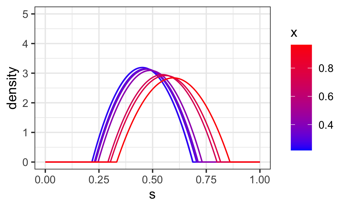
Figure 2: An example of $10$ response densities with randomly sampled predictor levels.

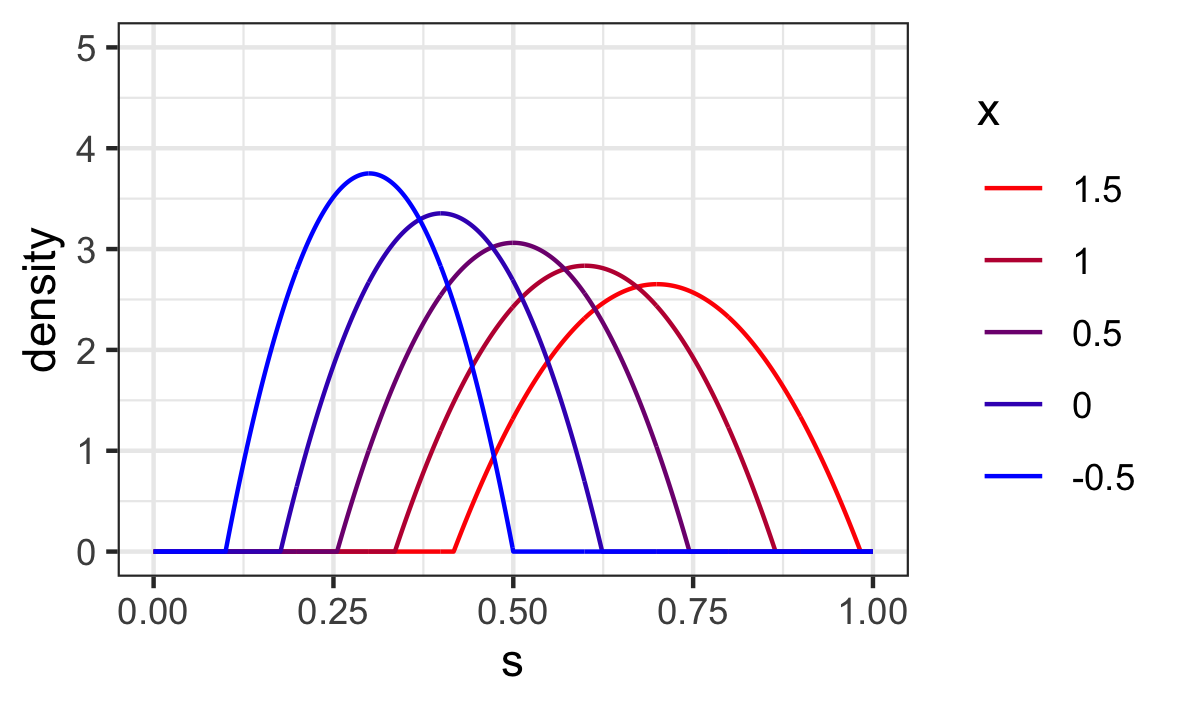
Figure 3: Left panel: Interpolating distributions obtained by fitting the global model. Right panel: True model, with $x=-0.5,0,0.5,1,1.5$. For $x=-0.5$ and $x=1.5$ the fits correspond to extrapolation, as $[0,1]$ is the predictor domain.

6.2 The two-dimensional case

For this simulation, we implemented the algorithm in section 3 and constructed distributions $\alpha|x$ that were obtained by Gaussians that were supplied with changing means and covariances in dependence on a variable $x\in[0,1]$, truncated on the compact support $[0,1]\times[0,1]$. A scalar predictor $X$ was generated from a uniform distribution on $[0,1]$, and the distributional trajectories as $\alpha|X=x\sim N((0.4x+0.3\quad 0.4x+0.3)^{T},\Sigma(x))$ with covariance matrix $\Sigma(x)=V\Lambda V^{\prime}$, where $V=\begin{bmatrix}\frac{\sqrt{2}}{2}&\frac{\sqrt{2}}{2}\\ -\frac{\sqrt{2}}{2}&\frac{\sqrt{2}}{2}\end{bmatrix}$, $\Lambda={\rm diag}(\lambda_{1},\lambda_{2})$ and $(\lambda_{1},\lambda_{2})|X=x\sim\frac{1}{100}N((1+0.5x\quad 1-0.5x)^{\prime},\,0.01\mathbf{I}_{2})$. It is easy to check that in this case the global model agrees with the true model. We performed simulation experiments for sample sizes $n=50,100,150,200$ on a $101$ by $101$ equidistant grid on $[0,1]\times[0,1]$, selecting the Sinkhorn regularization parameter as $\rho=\frac{2}{5}$.

The evaluation of the performance of the global model fit in the two-dimensional case is computationally expensive; due to the $101\times 101=10201$ grid, the cost and joint measure matrices have dimension $10201\times 10201$ and calculating the exact Wasserstein distance is extremely time consuming. It is therefore expedient to use a shortcut, the mean integrated Sinkhorn error (MISE),

$$\text{MISE}_{i}=E\int_{0}^{1}W_{2,\rho}^{2}(\hat{\mu}_{G}(x),\mu_{G}(x))dx,$$ (12)

where for $x\in[0,1]$, $\hat{\mu}_{G}(x)$ is the interpolation obtained from the global fit and for $x>1$ or $x<0$ these fits are extrapolations. Its empirical counterpart obtained from $M_{c}$ Monte Carlo runs is the empirical MISE,

$$\text{EMISE}_{i}=\frac{1}{M_{c}}\sum_{l=1}^{M_{c}}\int_{0}^{1}W_{2,\rho}^{2}(\hat{\mu}_{G,l}(x),\mu_{G}(x))dx.$$ (13)

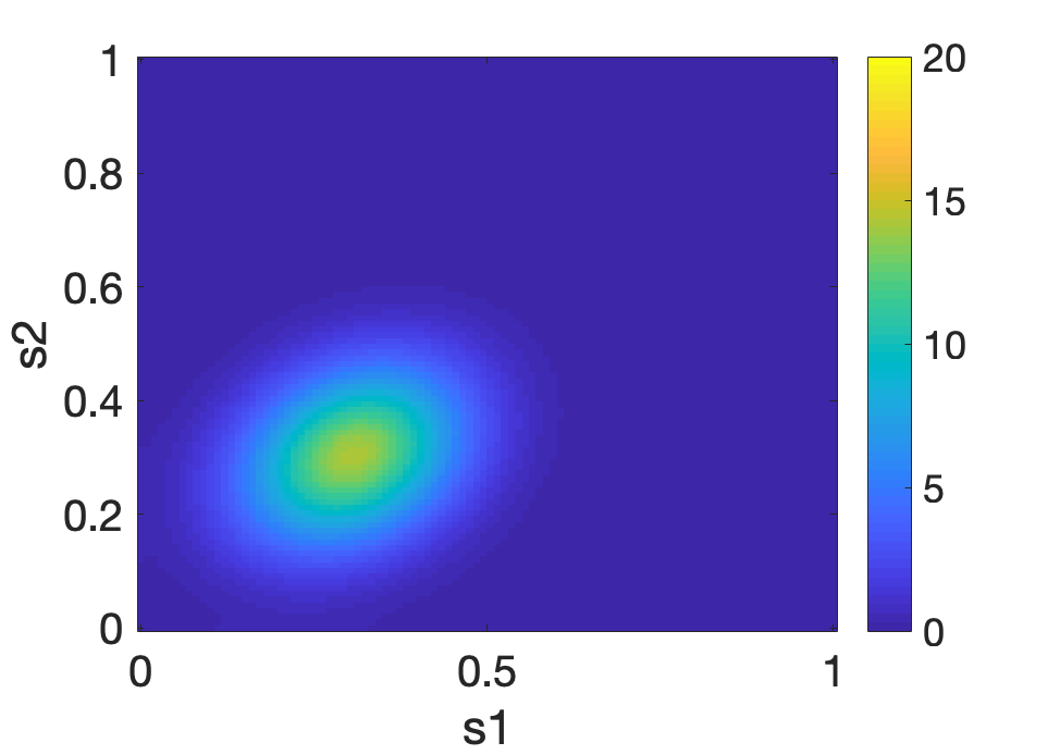
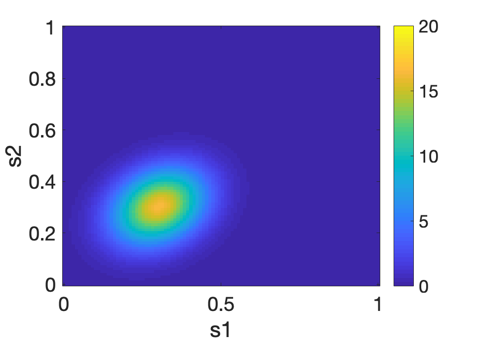
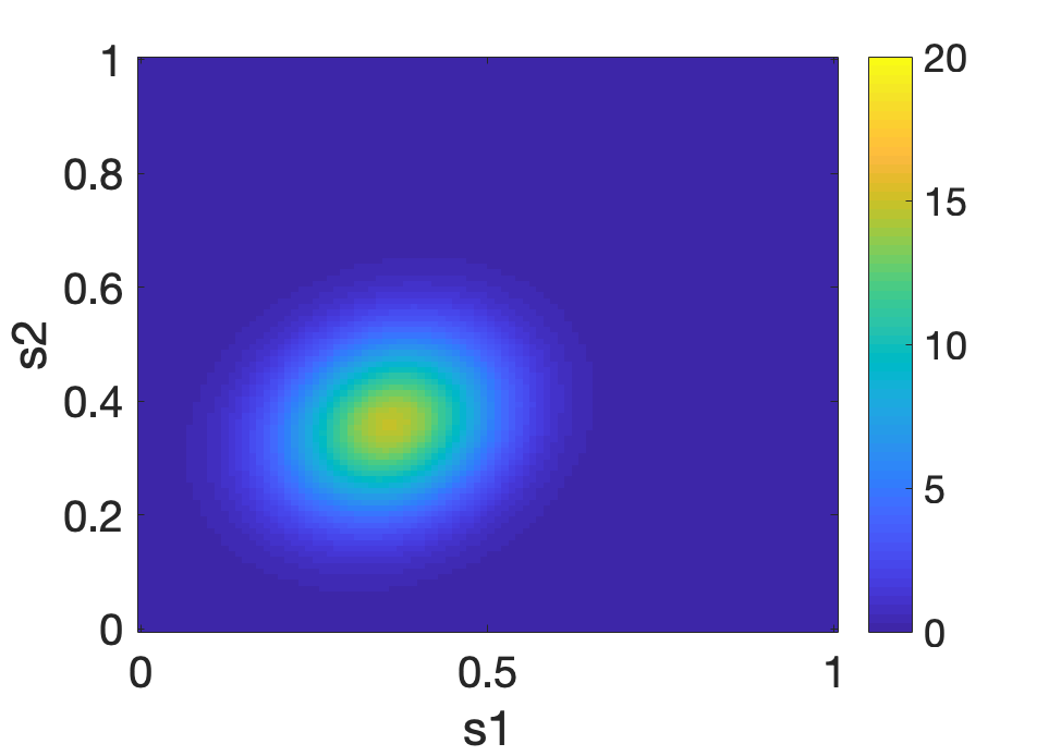
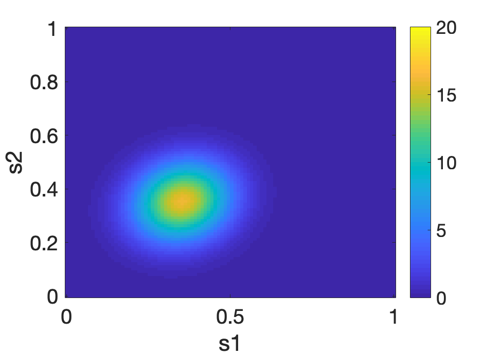
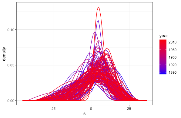
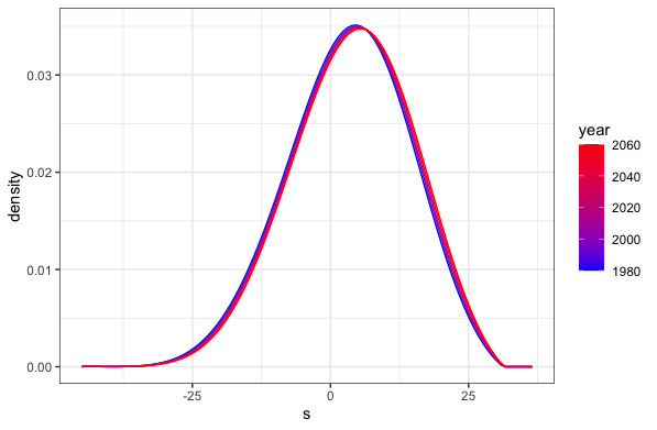
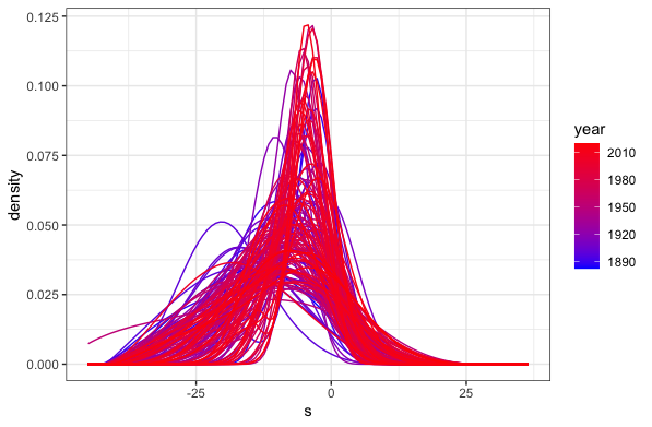
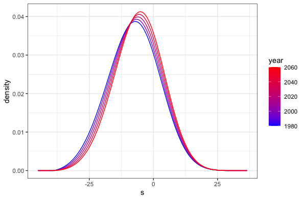
Figure 12: Left side side extrapolations obtained by fitting the global model (left panels) for 2-dimensional simulated data with $n=50$, where predictors are randomly sampled on $[0,1]$, and true extrapolated Wasserstein geodesic (right panels), for extrapolation levels at $x=-0.5$ (upper panels) and at $x=-0.5$ (lower panels).

Figure 13: Marginal densities of maximum and minimum temperature in March for Calgary, with the same layout as in Figure 9.

The results of the global fits are visualized in Figures 4 and 5, while those for extrapolation on the left side are in Figure 13. The local model fits for the same data are shown in Figure 6. This indicates that even for small sample sizes such as $n=50$ these fits work surprisingly well for both interpolation and extrapolation. The EMISEs of global and local fits for $100$ Monte Carlo runs with $\rho=\frac{2}{5}$ in Table 2 demonstrate that EMISE is dominated by the regularization parameter $\rho$; this conforms with the observation in Janati et al. (2020) that the weighted Sinkhorn barycenters are blurred compared with the actual Wasserstein barycenters.

Sample size	$n=50$	$n=100$	$n=150$	$n=200$
$\rho$	$\frac{1}{\rho}=5.5$	$\frac{1}{\rho}=4.5$	$\frac{1}{\rho}=3.5$	$\frac{1}{\rho}=2.5$
Global extrapolation	0.0448	0.0429	0.0413	0.0402
Global interpolation	0.0449	0.0432	0.0419	0.0408
Local interpolation	0.0449	0.0430	0.0414	0.0403

Table 2: EMISEs (13) for different sample sizes and methods for 2-dimensional distributions.

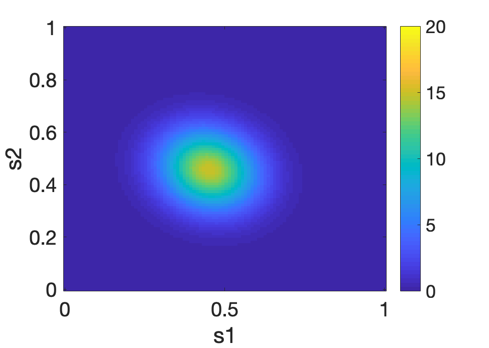
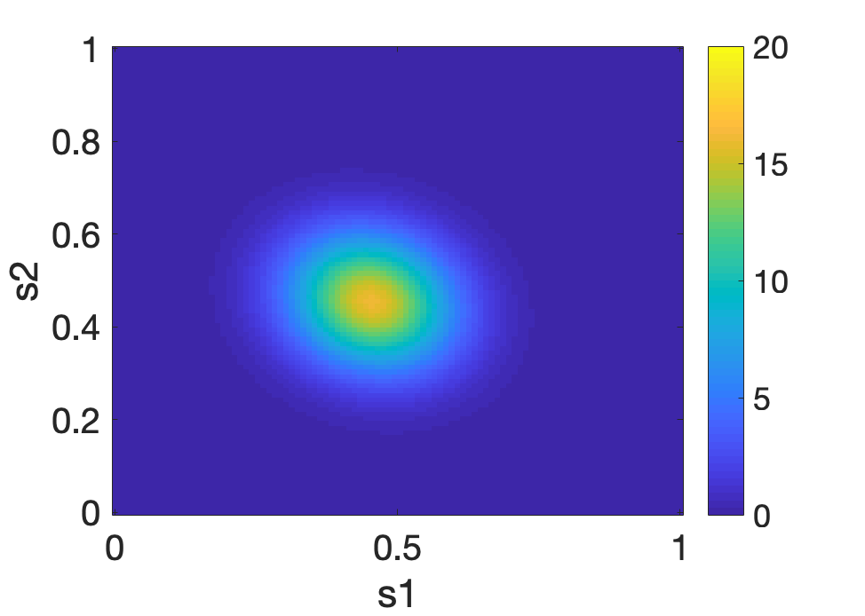
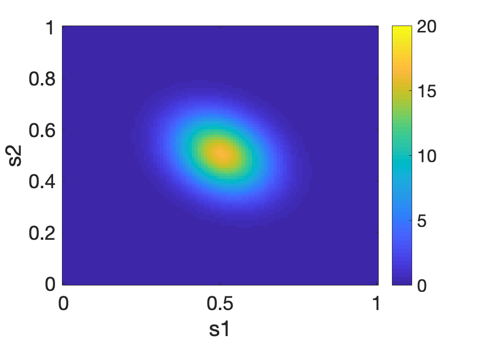
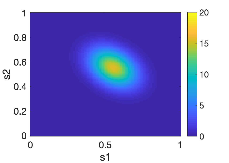
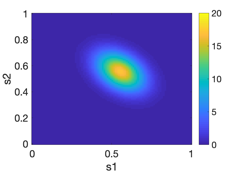
Figure 4: Interpolated distributions (left panels) obtained from fitting the global model for 2-dimensional distributions in the simulation setting described in the text with $n=50$ and exact Wasserstein geodesics (right panels), at predictor levels $x=0.25$ (top panels), $x=0.5$ (middle panels) and $x=0.75$ (bottom panels).

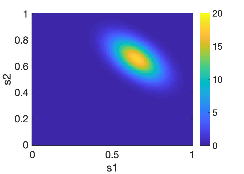
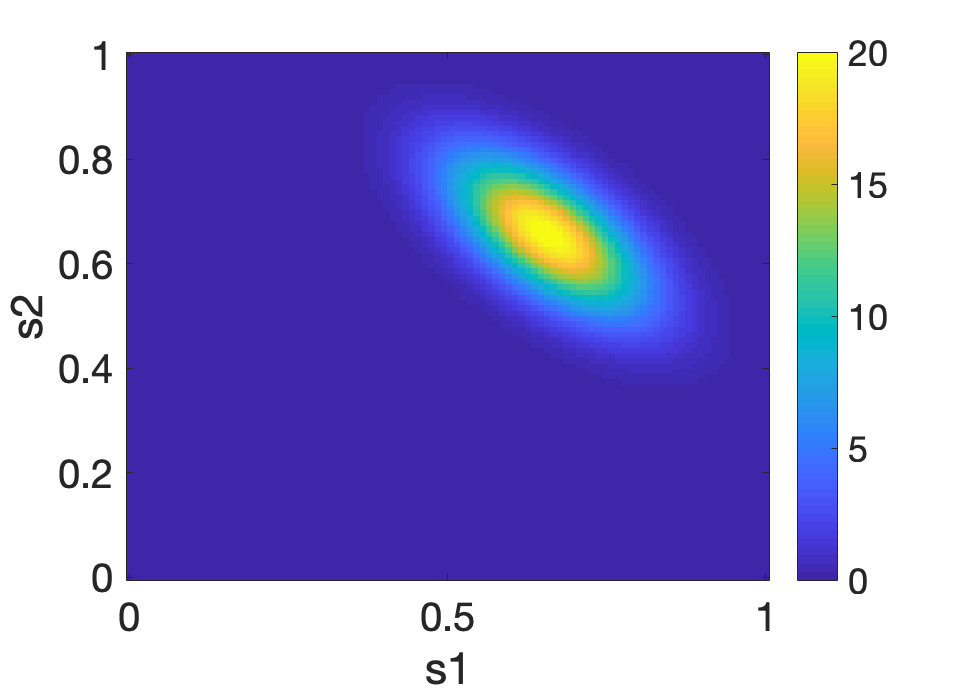
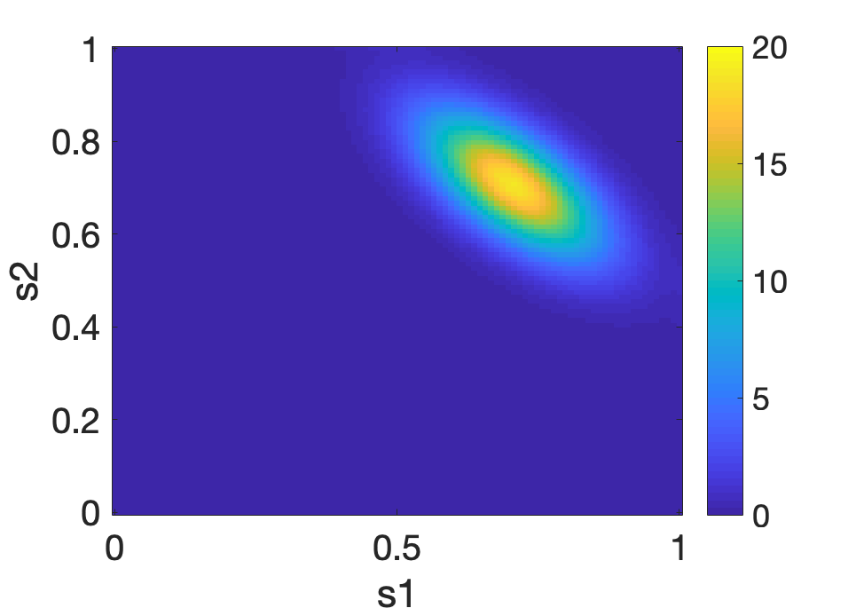
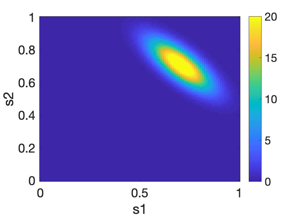
Figure 5: Right side extrapolations obtained by fitting the global model (left panels) for 2-dimensional simulated data with $n=50$, where predictors are randomly sampled on $[0,1]$. available in $[0,1]$, and true extrapolated Wasserstein geodesic (right panels), for mild extrapolation at $x=1.25$ (upper panels) and more extreme extrapolation at $x=1.5$ (lower panels).

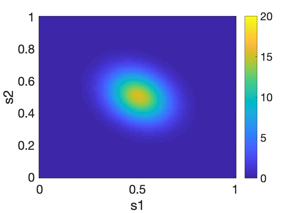
Figure 6: Interpolated distributions (left panels) obtained from fitting the local model for 2-dimensional distributions with $n=50$ and exact Wasserstein geodesics (right panels), at predictor levels $x=0.25$ (top panels), $x=0.5$ (middle panels) and $x=0.75$ (bottom panels).

Additional simulations for response distributions with heavier tails can be found in the Supplement.

7 Applications

7.1 BLSA data

The Baltimore Longitudinal Study of Aging (BLSA) data https://www.blsa.nih.gov/ contains various health data collected over a part of the lifespan of included individuals. We extracted systolic (SBP) and diastolic blood pressure (DBP) measurements, where $8000$ measurements (age of the individual at the time of the measurement, SBP and DBP) were available for $2801$ individuals. The number of visiting times for an individual varies from $1$ to $26$ and the range of ages at which measurements were recorded is $[17,75]$. Here we use age as predictor and construct the density responses by kernel density estimators for the joint distribution of SBP and DBP, where in a preprocessing step the data is binned by age at the time of measurements over $20$ equidistant bins between $30$ to $75$; the bandwidth for the kernel smoothing step was chosen using the method of Sheather and Jones (1991), for both this as well as the following data illustration. The joint 2-dimensional densities were estimated over $51$ equidistant grid points in each direction over the domain $[30,130]$ for SBP and $[70,210]$ for DSP.

The distributional fits from the global model in Figure 7 for ages $x=5,25,85,105$ demonstrate distributional extrapolation and for ages $x=45,65$ distributional interpolation. There is a clear indication of a distributional trend towards higher systolic and diastolic blood pressures as age grows, as well as increasing spread. At age $5$ the mode is around $60,120$ and at age $105$ around $90,150$. The interpolated and extrapolated distributions are concentrated around the diagonal running from $(30,70)$ to $(130,210)$ with the3 exception of age $5$. With increasing age, the covariance of the distribution increases considerably, while there are indications that the correlation of SBP/DSP is quite stable across age.

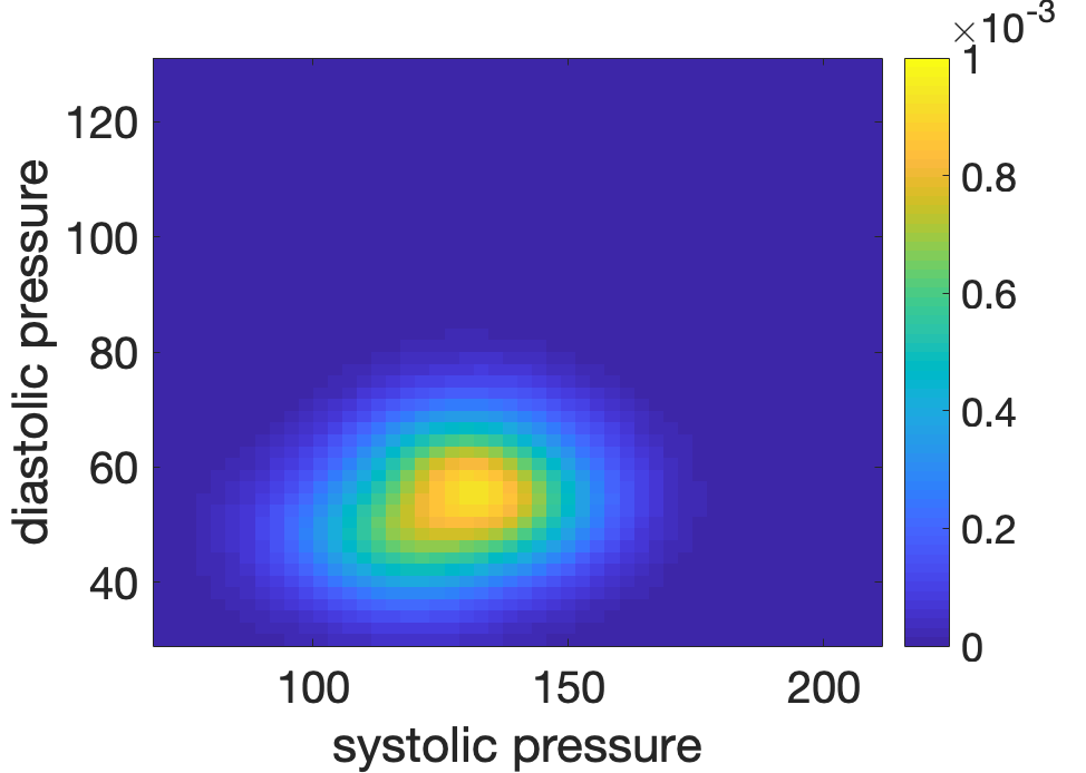
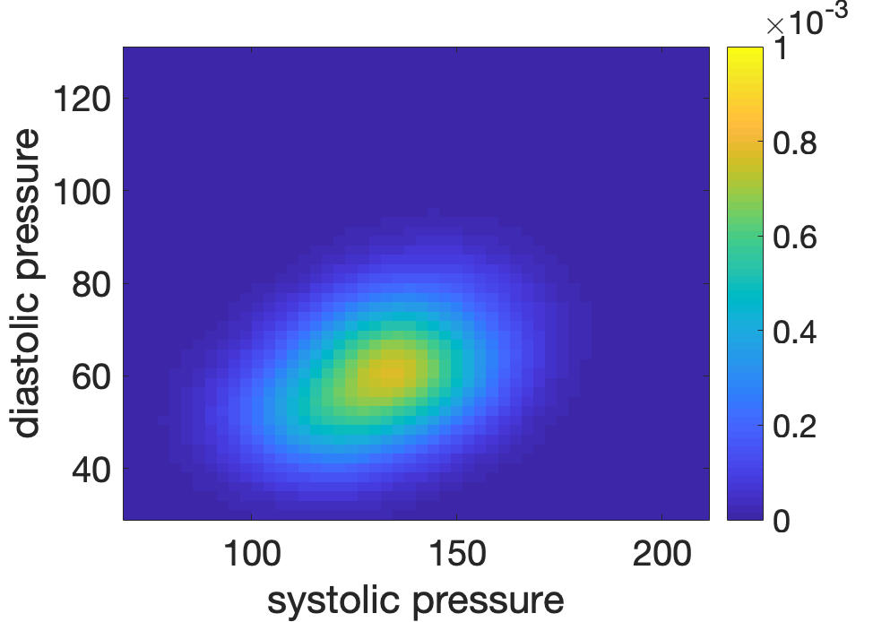
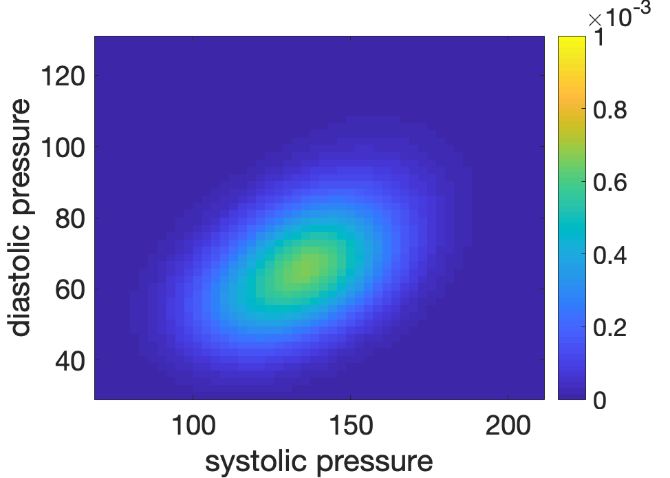
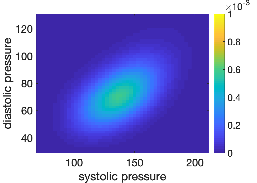
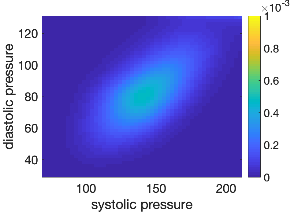
Figure 7: Applying global fitting to the joint (SBP/DBP) distributions for the BLSA data with distributions at $20$ different age bins as inputs. The first row displays the fits for ages $5,25$ (left extrapolation), the second row for ages $45,65$ (interpolation) and the third row for ages $85,105$ (right extrapolation).

7.2 Calgary temperature data

These data, available at https://calgary.weatherstats.ca/, consist of recordings of the minimum and maximum temperature for each day from $1882$ to $2020$ in Calgary (Alberta). For each year, we constructed the joint distribution of minimum and maximum temperatures recorded daily for January, March and June and used kernel density estimation to obtain estimates for both joint and marginal distributions, both marginally and jointly. For the marginal distributions both the distributions of minimum and maximum temperature were targeted. For the joint distribution, a more expedient way turned out to work with the joint two-dimensional distribution of minimum temperature recorded for a given day and the difference between maximum and minimum temperatures recorded for the same day, the latter corresponding to the observed temperature range, as this simple linear data transformation made it possible to use the same rectangular support for all distributions considered.

We first fitted the global model for the marginal one-dimensional density responses and year as predictor to obtain predictions for the future distribution of maximum and minimum temperatures through the proposed Wasserstein extrapolation. The fitted distributions in Figures 9 (for January), 9 (for June) and 13 (for March, in the Supplement) indicate that the fitted distribution of the minimum temperature in March and June varies very little over calendar time and while generally the maximum and minimum temperatures are predicted to move toward higher values, the maximum temperature in June trends smaller with increasing extrapolation year.

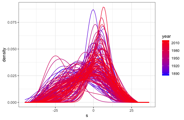
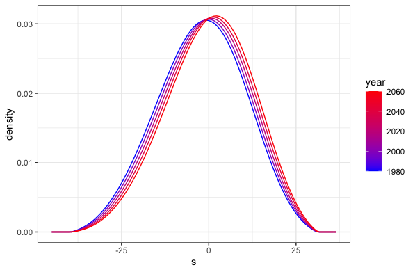
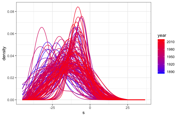
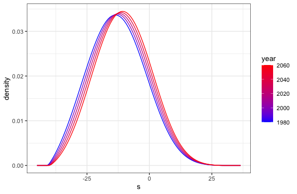
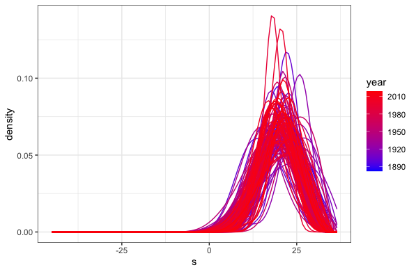
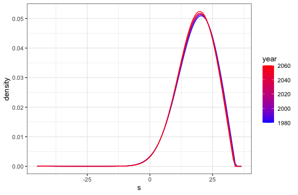
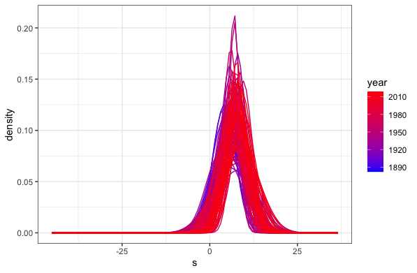
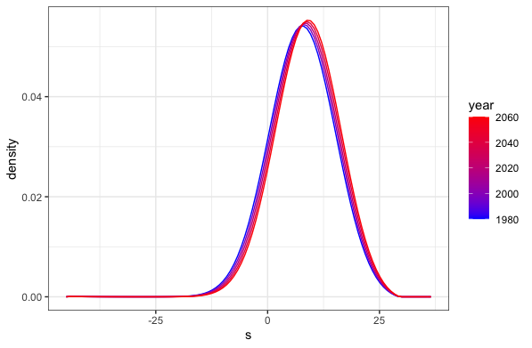
Figure 8: Calgary temperature data. Marginal distributions of maximum (upper panels) and minimum (lower panels) temperature in January, with observed (kernel smoothed) densities for these distributions (left panels) and extrapolated global fits (right panel) for $1980,2000,2020,2040,2060$. The densities are color coded by calendar year.

Figure 9: Calgary temperature data. Marginal distributions of maximum and minimum temperature in June, with the same layout as the previous figure.

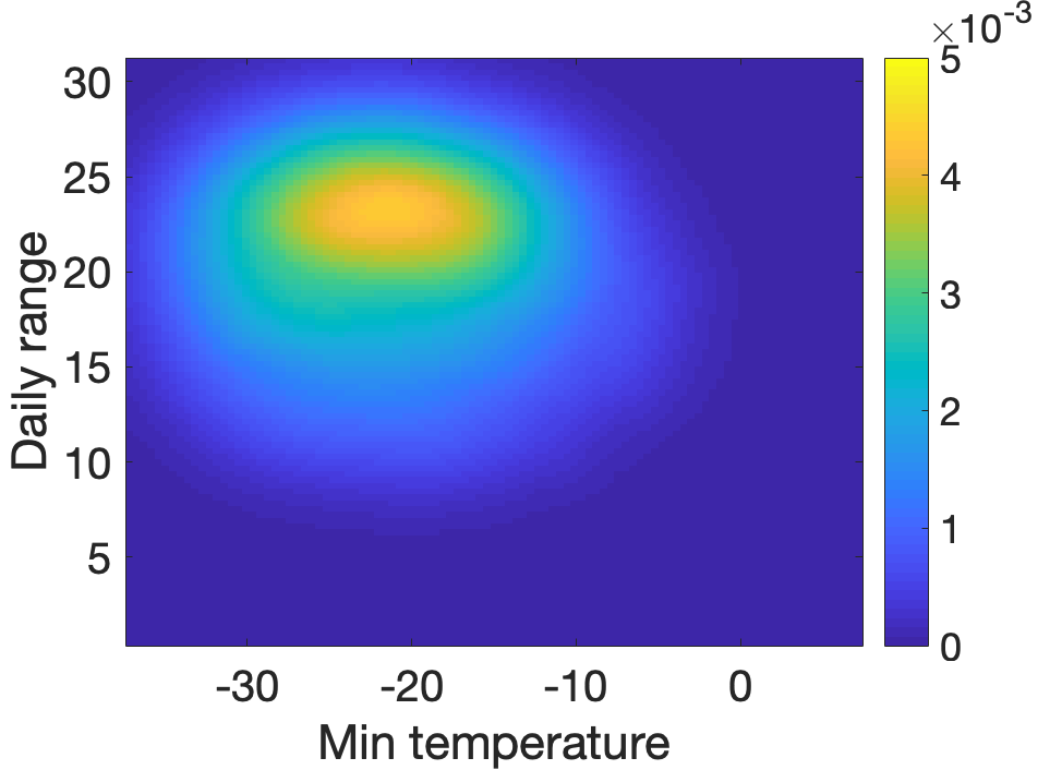
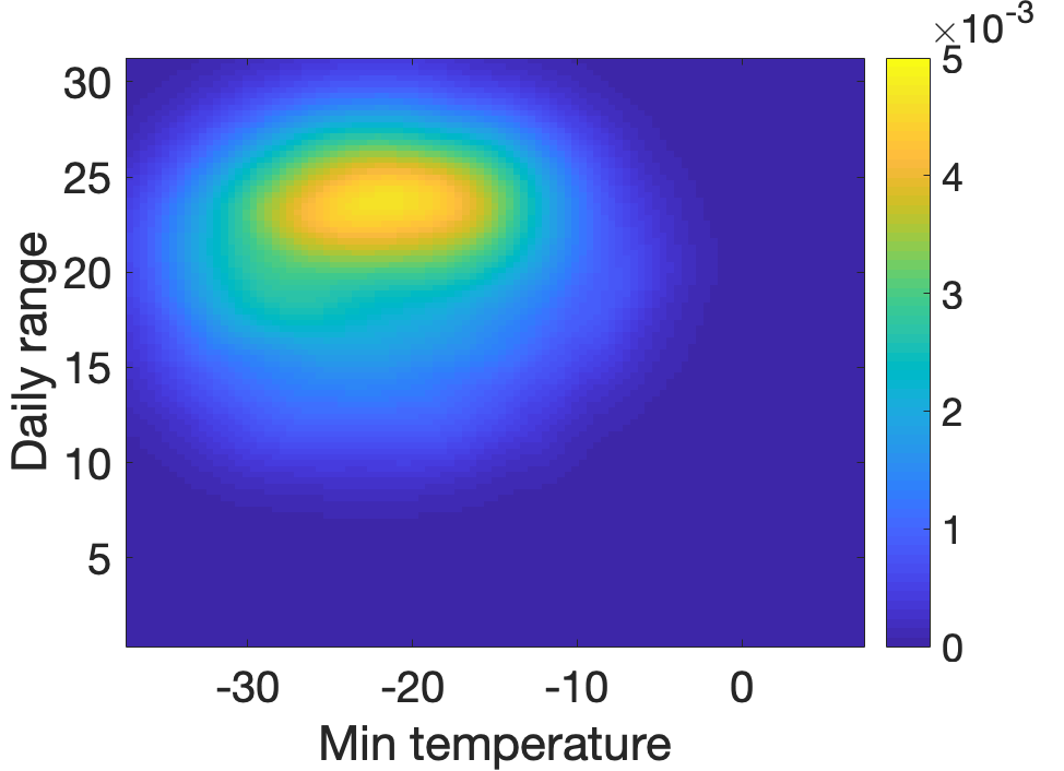
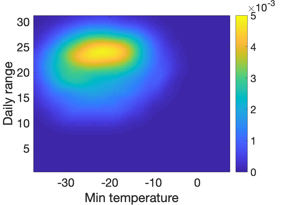
Figure 14: Globally fitted joint distributions of the maximum-minimum (temperature range) and the minimum temperature in March. First row: Extrapolation for the years $1980$. Second row: For the years $2000,2020$. Third row: For the years $2040,2060$.

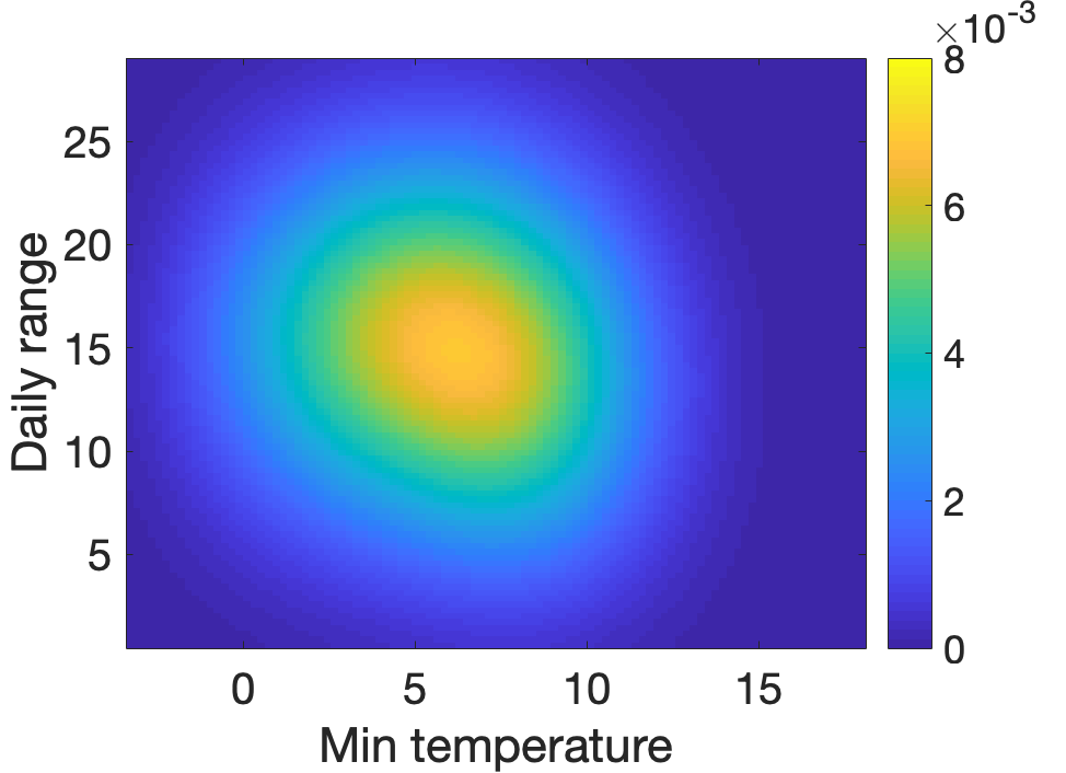
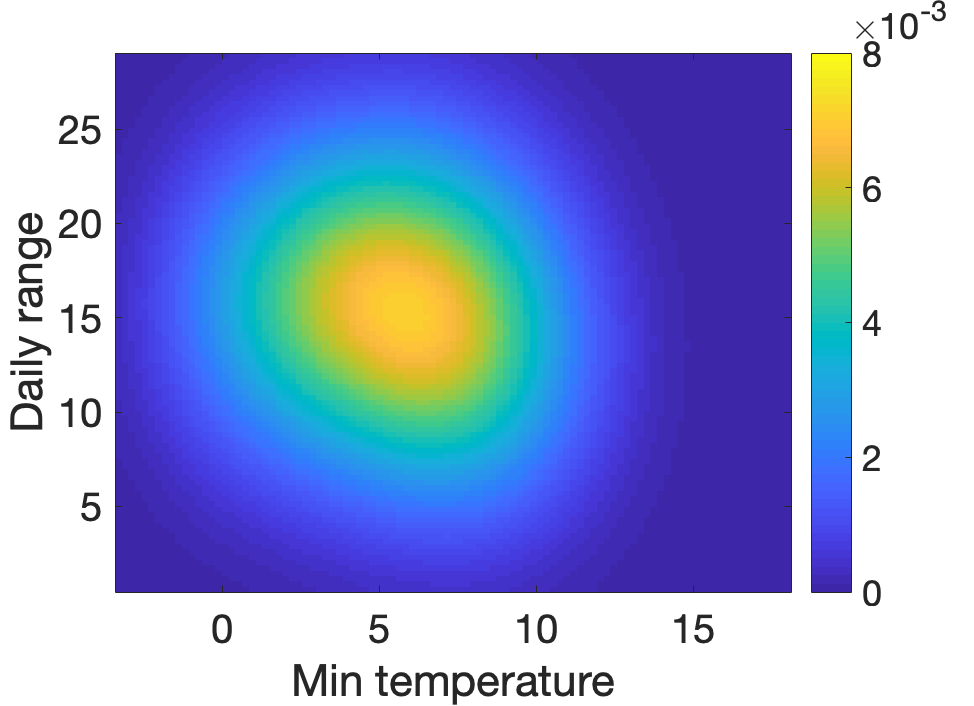
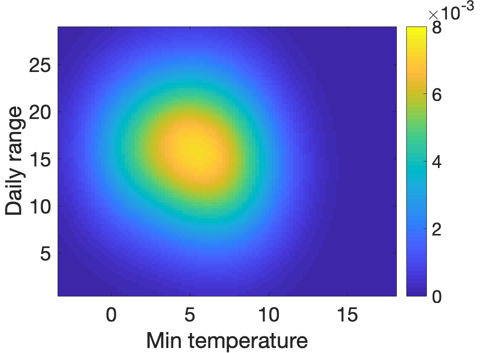
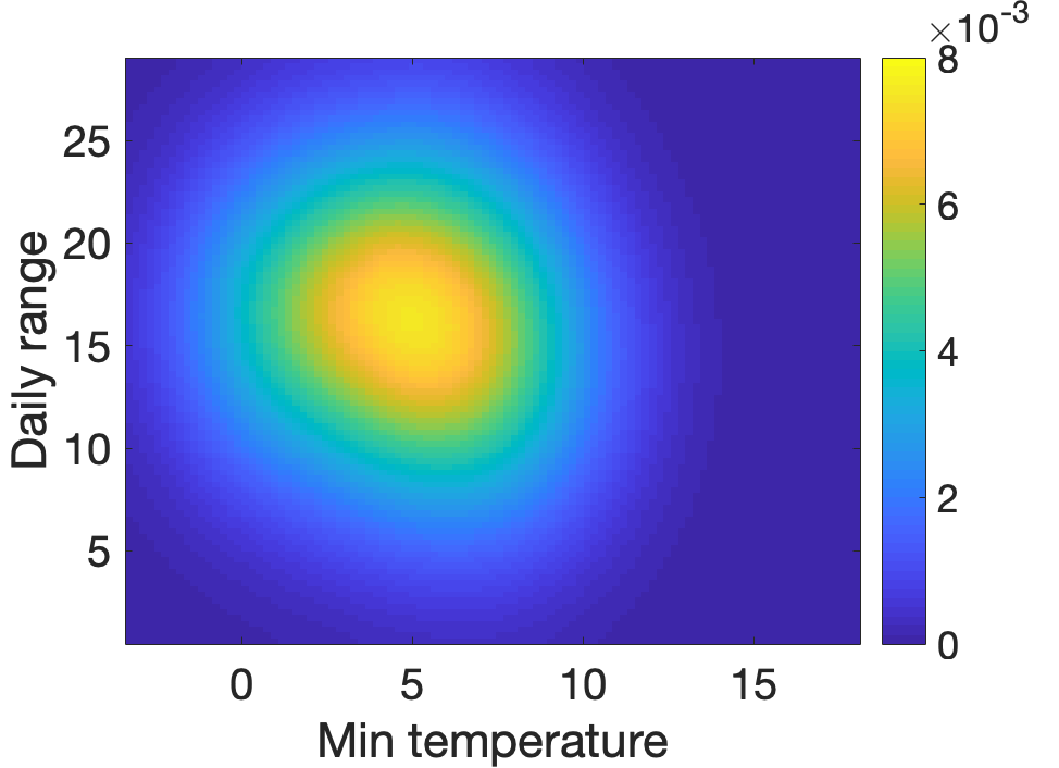
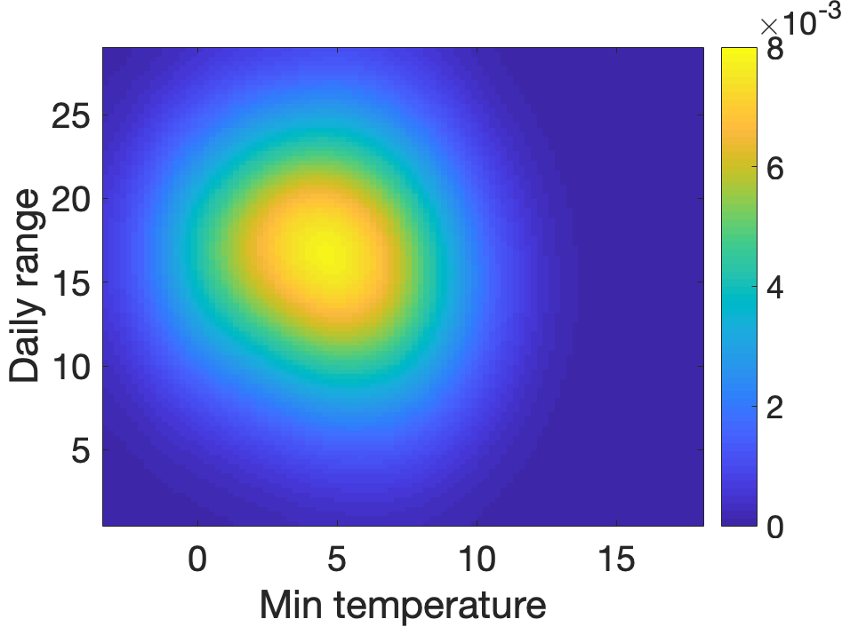
Figure 15: Same as Figure 14 for June.

The fits with the global model of two-dimensional densities of maximum-minimum temperature and minimum temperature shown for January in Figure 10 and for March and June in Figures 13, 14 and 15 (in the Supplement) indicate that for March the primary change over calendar time is in terms of the location of the fitted joint distribution, where the minimum temperature is increasing, as shown in Figure 13. As for shape changes, the fitted joint distribution tends towards a decreased variance in the $s_{2}-s_{1}$ direction, where $s_{1}$ and $s_{2}$ are the $x$ and $y$ axes in the two dimensional distribution. For June the changes in the two-dimensional distributions are barely noticeable, which also agrees with the marginal one-dimensional fits displayed in Figure 9. For January, the location of the joint distribution does not have an obvious shift but there is an interesting finding that the joint distribution tends to develop a weak second mode that involves a smaller daily temperature range in the extrapolation towards future calendar years.

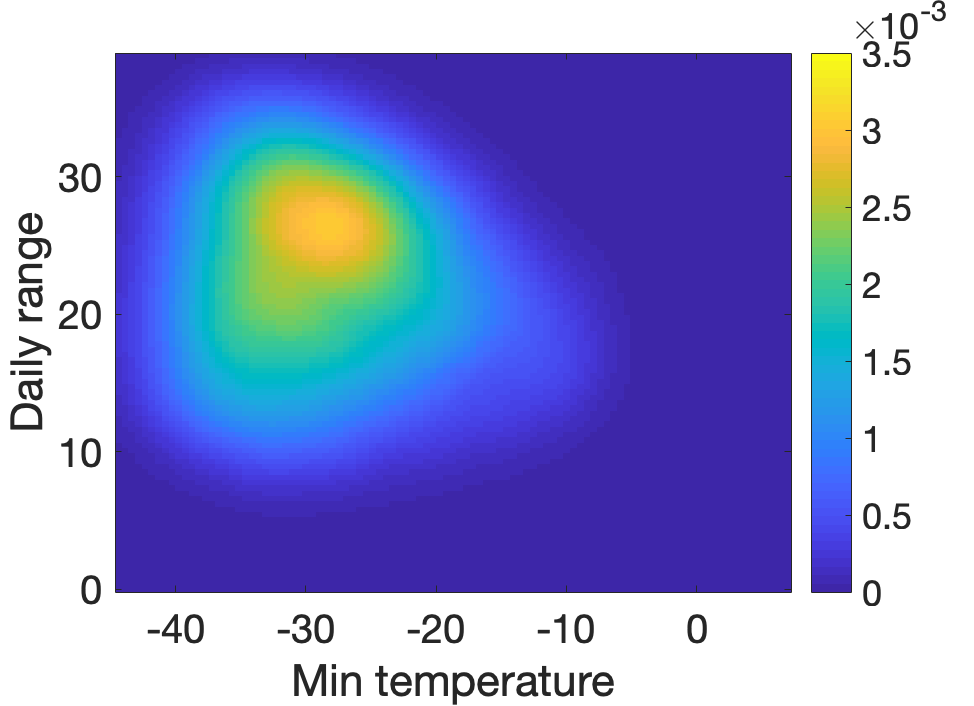
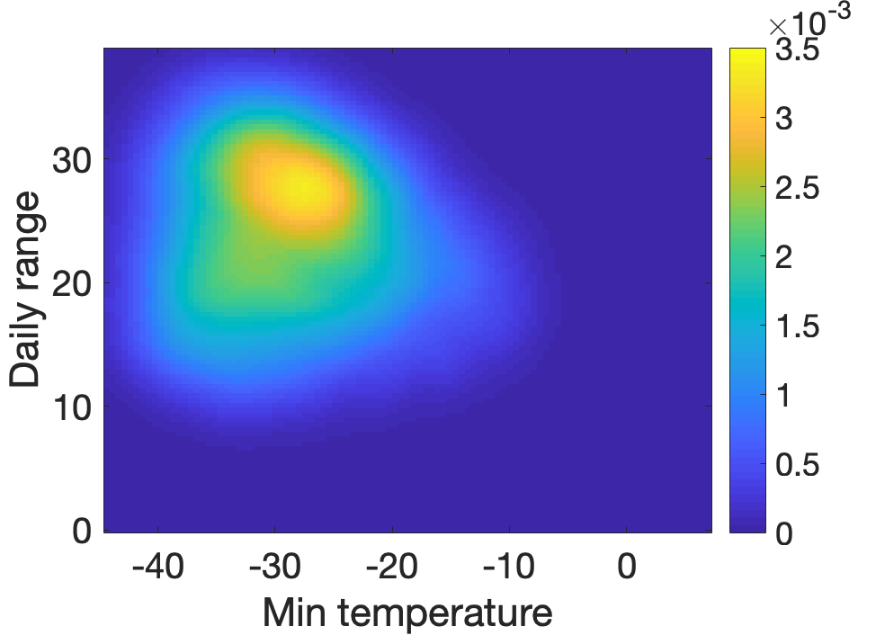
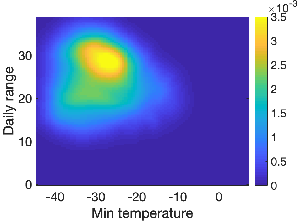
Figure 10: Global fits for the joint distribution of maximum-minimum (range) and minimum temperature in Calgary for January, extrapolating to $1980$ (first row), $2000,2020$ (second row) and $2040,2060$ (third row).

8 Proofs and Auxiliary Results

8.1 Proof of Proposition 1

Proof.

We prove the results for the global estimates here, the generalization to local estimates is then straightforward.

By definition $\hat{\mu}_{G}(x)=\operatorname*{arg\,min}_{\mu\in\Omega}\frac{1}{m}\sum_{i=1}^{n}s_{iG}(x)W_{2}^{2}(\mu,\nu_{i})$ where in the 1-d case $W_{2}^{2}(\mu_{1},\mu_{2})=\int_{0}^{1}(F^{-1}_{\mu_{1}}(t)-F^{-1}_{\mu_{2}}(t))^{2}dt$, we have

$$F^{-1}_{\hat{\mu}_{G}(x)}(t)=\operatorname*{arg\,min}_{Q\in\mathcal{Q}}\frac{1}{n}\sum_{i=1}^{n}s_{iG}(x)\int_{0}^{1}(F^{-1}_{\nu_{i}}(t)-Q)^{2}dt.$$

Then observing $\frac{1}{n}\sum_{i=1}^{n}s_{iG}(x)=1$,

$$\frac{1}{n}\sum_{i=1}^{n}s_{iG}(x)\int_{0}^{1}(F^{-1}_{\nu_{i}}(t)-F^{-1}_{\mu}(t))^{2}dt = \int_{0}^{1}(F^{-1}_{\mu}(t)^{2}-\frac{2}{n}(\sum_{i=1}^{n}s_{iG}(x)F^{-1}_{\nu_{i}}(t))F^{-1}_{\mu}(t))dt+C_{1}$$

$$= \int_{0}^{1}(F^{-1}_{\mu}(t)-\frac{1}{n}\sum_{i=1}^{n}s_{iG}(x)F^{-1}_{\nu_{i}}(t))^{2}dt+C_{2},$$

where $C_{1},C_{2}$ are constants. This implies $F^{-1}_{\hat{\mu}_{G}(x)}(t)=\operatorname*{arg\,min}_{Q\in\mathcal{Q}}\|Q-\frac{1}{n}\sum_{i=1}^{n}s_{iG}(x)F^{-1}_{\nu_{i}}(t)\|$ and completes the proof. ∎

8.2 Proof of Proposition 2

Proof.

The proof proceeds by constructing a histogram $H$ such that $W_{2}^{2}(\nu_{H},\nu_{f})$ and $W_{2}^{2}(\nu_{H},\nu_{\mathbf{r}})$ is of the desired order. where $\nu_{H},\nu_{f}$ are continuous measures with density $H$ and $f$ and $\nu_{\mathbf{r}}$ is the discrete measure on $(d_{1},\ldots,d_{m})$ with probability mass $\mathbf{r}$. In the first step we construct such a histogram. Let $(R_{1},\ldots,R_{m})$ be the small rectangles created by the grid such that $d_{k}$ is the vertex of rectangular bin $R_{k}$ with smallest coordinates in all directions. If $d_{k}$ reaches the largest value of one coordinate, we can extend the grid so that this rectangle can be included. These rectangles serve as bins of the histogram. Then $H$ is the histogram on these bins with frequencies $(\frac{f_{i}(d_{1})}{\sum_{j=1}^{m}f_{i}(d_{j})},\frac{f_{i}(d_{2})}{\sum_{j=1}^{m}f_{i}(d_{j})},\ldots,\frac{f_{i}(d_{m})}{\sum_{j=1}^{m}f_{i}(d_{j})})$. Let $d_{TV}(\mu_{1},\mu_{2})=\sup_{B\subset\mathbb{R}^{d}}|\mu_{1}(B)-\mu_{2}(B)|$ be the total variation distance, by Lipschitz continuity we immediately get $d_{TV}(\nu_{H},\nu_{f})=O(\zeta)$. It has been proved in Gibbs and Su (2002) that $d_{P}(\mu_{1},\mu_{2})\leq d_{TV}(\mu_{1},\mu_{2})$, where $d_{P}$ is the Prokhorov distance. For any joint distribution $J$ of random variables $X,Y$ with marginals $\mu,\nu$,

$$E_{J}\|X-Y\|^{2} \leq \epsilon^{2}P(\|X-Y\|^{2}\leq\epsilon^{2})+\text{diam}(M)P(\|X-Y\|^{2}>\epsilon^{2})$$

$$= \epsilon^{2}+(\text{diam}(M)-\epsilon^{2})P(\|X-Y\|^{2}>\epsilon^{2}).$$

If $d_{P}(\mu,\nu)\leq\epsilon$, we can choose a coupling $J_{1}$ so that $P(\|X-Y\|^{2}>\epsilon^{2})\leq\epsilon$ (Huber (2004),p.27). Thus,

$$E_{J_{1}}\|X-Y\|^{2}\leq\epsilon^{2}+(\text{diam}(M)-\epsilon^{2})\epsilon\leq\epsilon^{2}+\text{diam}(M)\epsilon$$

and therefore

$$W_{2}^{2}(\mu,\nu) \leq E_{J_{1}}[\|X-Y\|^{2}]\leq d_{P}(\mu,\nu)^{2}+\text{diam}(M)d_{P}(\mu,\nu)\leq d_{TV}^{2}(\mu,\nu)$$

$$+\text{diam}(M)d_{TV}(\mu,\nu).$$

We conclude $W^{2}_{2}(\nu_{H},\nu_{f})=O(d_{TV}(\mu,\nu)+d_{TV}^{2}(\mu,\nu))=O(\zeta)$. Next we prove $W_{2}^{2}(\nu_{H},\nu_{\mathbf{r}})=o(\zeta^{2})$. To do this we construct a push-forward map $\tilde{T}$ from $\nu_{H}$ to $\nu_{\mathbf{r}}$ such that it maps each bin $R_{k}$ to the vertex $d_{k}$. It is obvious that $\tilde{T}_{\#}\nu_{H}=\nu_{\mathbf{r}}$ as the probability in each bin $R_{k}$ equals the probability mass of the corresponding vertex $d_{k}$. By definition of the 2-Wasserstein distance,

$$W_{2}^{2}(\nu_{H},\nu_{f})\leq\int_{M_{0}}\|\tilde{T}(w)-w\|^{2}d\nu_{H}\leq\int_{M_{0}}\zeta^{2}d\nu_{H}=\zeta^{2}=O(\zeta^{2}),$$ (15)

where $M_{0}=\cup_{j=1}^{m}R_{j}$. Combining these two results we have
$W_{2}^{2}(\nu_{\mathbf{r}},\nu_{f})\leq 2(W_{2}^{2}(\nu_{H},\nu_{f})+W_{2}^{2}(\nu_{H},\nu_{\mathbf{r}}))=O(\zeta)$. ∎

8.3 Proof of Theorem 1

Proof.

Since the weights $s_{G}(X,x)=s_{G}(U,u_{0})$ if $X=U\mathbf{c}+\mathbf{b},x=u_{0}\mathbf{c}+\mathbf{b}$, we only consider the case $X=U$ and $x=u_{0}$. First we consider the case $u_{0}\in[0,1]$; the extrapolation case can be handled analogously. W.L.O.G. assume $E(U)\leq u_{0}$. If $u_{0}=E(U)$, let $u^{*}=0$. Otherwise $s_{G}(u,u_{0})$ is linear in $u$ with positive slope, so there exists $u_{1}$ be such that $s_{G}(u_{1},u_{0})=0$. In this case define $u^{*}=\max(u_{1},0)$. It is easy to see $u^{*}<u_{0}$, as $s_{G}(u_{0},u_{0})=1+(u_{0}-E(U))^{2}/{\rm Var}(U)>0$. Because of the positive slope and linearity of the weights, it holds for any $u$ that $\mathbf{1}_{\{u\in[0,u^{*})\}}s_{G}(u,u_{0})\leq 0$ and $\mathbf{1}_{\{u\in[u^{*},1]\}}s_{G}(u,u_{0})\geq 0$, where $\mathbf{1}$ is the indicator function. Denote $\theta=W_{2}(\tilde{\nu}(0),\tilde{\nu}(1))$. For $u<u^{*}$, $W_{2}(\mu,\tilde{\nu}(u))\leq W_{2}(\mu,\tilde{\nu}(u^{*}))+W_{2}(\tilde{\nu}(u^{*}),\tilde{\nu}(u))$ and for $u\geq u^{*}$, $|W_{2}(\mu,\tilde{\nu}(u))|\geq|W_{2}(\tilde{\nu}(u^{*}),\mu)-W_{2}(\tilde{\nu}(u),\tilde{\nu}(u^{*}))|$. With $W_{2}(\tilde{\nu}(u),\tilde{\nu}(u^{*}))=|u-u^{*}|\theta$, we have that for any $\mu$

$$E[s_{G}(U,u_{0})W_{2}^{2}(\mu,\tilde{\nu}(U))\mathbf{1}_{\{U\in[0,u^{*})\}}]$$

$$\geq E[s_{G}(U,u_{0})(W_{2}(\mu,\tilde{\nu}(u^{*}))+W_{2}(\tilde{\nu}(u^{*}),\tilde{\nu}(U)))^{2}\mathbf{1}_{\{U\in[0,u^{*})\}}]$$

$$= E[s_{G}(U,u_{0})(W_{2}(\mu,\tilde{\nu}(u^{*}))+(u^{*}-U)\theta)^{2}\mathbf{1}_{\{U\in[0,u^{*})\}}]$$

and

$$E[s_{G}(U,u_{0})W_{2}^{2}(\mu,\tilde{\nu}(U))\mathbf{1}_{\{U\in[u^{*},1]\}}]$$

$$\geq E[s_{G}(U,u_{0})(W_{2}(\mu,\tilde{\nu}(u^{*}))-W_{2}(\tilde{\nu}(U),\tilde{\nu}(u^{*})))^{2}\mathbf{1}_{\{U\in[u^{*},1]\}}]$$

$$= E[s_{G}(U,u_{0})(W_{2}(\mu,\tilde{\nu}(u^{*}))-(U-u^{*})\theta)^{2}\mathbf{1}_{\{U\in[u^{*},1]\}}],$$

where equality is achieved when $\mu=\tilde{\nu}(\tilde{u})$ with $\tilde{u}>u^{*}$.

Combining the results above with $E(s_{G}(U,u_{0}))=1$, one finds that for any $\mu$

$$E(s_{G}(U,u_{0})W_{2}^{2}(\mu,\tilde{\nu}(U)))$$

$$= E[s_{G}(U,u_{0})W_{2}^{2}(\mu,\tilde{\nu}(U))\mathbf{1}_{\{U\in[0,u^{*})\}}]+E[s_{G}(U,u_{0})W_{2}^{2}(\mu,\tilde{\nu}(U))\mathbf{1}_{\{U\in[u^{*},1]\}}]$$

$$\geq E[s_{G}(U,u_{0})(W_{2}(\mu,\tilde{\nu}(u^{*}))+(u^{*}-U)\theta)^{2}\mathbf{1}_{\{U\in[0,u^{*})\}}]$$

$$+E[s_{G}(U,u_{0})(W_{2}(\mu,\tilde{\nu}(u^{*}))-(U-u^{*})\theta)^{2}\mathbf{1}_{\{U\in[u^{*},1]\}}]$$

$$= E[s_{G}(U,u_{0})(W_{2}(\mu,\tilde{\nu}(u^{*}))+(u^{*}-U)\theta)^{2}]$$

$$= E(s_{G}(U,u_{0}))EW_{2}^{2}(\mu,\tilde{\nu}(u^{*}))+2\theta E[(u^{*}-U)s_{G}(U,u_{0})]E[W_{2}(\mu,\tilde{\nu}(u^{*}))]+C_{1}$$

$$= EW_{2}^{2}(\mu,\tilde{\nu}(u^{*}))+2\theta E[(u^{*}-U)s_{G}(U,u_{0})]EW_{2}(\mu,\tilde{\nu}(u^{*}))+C_{1}$$

$$= (W_{2}(\mu,\tilde{\nu}(u^{*}))+\theta E[(u^{*}-U)s_{G}(U,u_{0})]))^{2}+C_{2},$$

where $C_{1},C_{2}$ are constants that do not depend on $\mu$. Then observing

$$E((u^{*}-U)s_{G}(U,u_{0}))$$

$$= E(u^{*}-U)+E((U-E(U))(u_{0}-E(U))/{\rm Var}(U))u^{*}-E(U(U-E(U))(u_{0}-E(U))/{\rm Var}(U))$$

$$= u^{*}-E(U)-(u_{0}-E(U))$$

$$= u^{*}-u_{0},$$

the minimum is achieved when $\mu$ is on the geodesic and $W_{2}(\mu,\tilde{\nu}(u^{*}))=(u_{0}-u^{*})\theta$. This implies $\hat{\mu}_{G}(u_{0})=\tilde{\nu}(u_{0})$. For the extrapolation case we simply replace $0$ by $t_{1}$ and $1$ by $t_{2}$ in the proof. ∎

8.4 Proof of Theorem 2

Proof.

This proof uses Theorem 2 in Petersen and Müller (2019), and the conditions necessary to apply this result that must be established first. The three conditions are

(P0) The objects $\mu_{G}(x)$ and $\hat{\mu}_{G}(x)$ exist and are unique, the latter almost surely. Additionally, for any $\epsilon>0$, $\inf_{W_{2}(\mu,\mu_{G}(x))>\epsilon}E(s_{G}(X,x)W_{2}^{2}(\mu,\nu))>E(s_{G}(X,x)W_{2}^{2}(\mu_{G}(x),\nu))$.

(P1) For $\delta>0$ small enough,

$$\int_{0}^{1}\sqrt{1+\log N(\delta\epsilon,B_{\delta}(\mu_{G}(x)),W_{2})}d\epsilon<\infty,$$

where $B_{\delta}(\mu_{G}(x),W_{2})$ is the $\delta$-ball in 2-Wasserstein space centered at $\mu_{G}(x)$ and $N(\epsilon,\Omega,d)$ is the covering number for $\Omega$ using open balls for radius $\epsilon$.

(P2) There exists $\eta>0,A>0$ and $\beta>1$, possibly depending on $x$, such that whenever
$W_{2}(\mu_{G}(x),\mu)<\eta$, we have
$E(s_{G}(X,x)W_{2}^{2}(\mu,\nu))-E(s_{G}(X,x)W_{2}^{2}(\mu_{G}(x),\nu))-AW_{2}(\mu,\mu_{G}(x))^{\beta}\geq 0$.

Under conditions (P0)-(P2), it then holds that

$$W_{2}(\hat{\mu}_{G}(x),\mu_{G}(x))=O_{p}(n^{-1/(2(\beta-1))}).$$ (16)

In the following, we will verify these conditions for $\beta=2$. We first prove (P1) by establishing an inequality that provides a bound for the covering number. We use that by (8.2) one has the bound $W_{2}^{2}(\mu,\nu)=O(d_{TV}(\mu,\nu))=O(\|f_{1}-f_{2}\|_{\infty})$. Then we use the fact that by Theorem 2.7.1 of van der Vaart and Wellner (1996), if $M$ is a bounded, convex subset of $\mathbb{R}^{d}$ with nonempty interior, there exists a constant $A_{1}$ depending only on $\gamma$ and $d$ such that

$$\log N(\epsilon,\mathcal{F}_{\gamma},\|\|_{\infty})\leq A_{1}(\frac{1}{\epsilon})^{\frac{d}{\gamma}}$$ (17)

for every $\epsilon>0$ .

Applying $W_{2}^{2}(\mu,\nu)=O(\|f_{1}-f_{2}\|_{\infty})$, we have $B_{A_{2}\epsilon}(\mu,\|\|_{\infty})\subset B_{\sqrt{\epsilon}}(\mu,W_{2})$ for some constant $A_{2}$ and $N(\epsilon,\mathcal{F}_{\gamma},W_{2})\leq A_{3}N(\epsilon^{2},\mathcal{F}_{\gamma},\|\|_{\infty})$ with a constant $A_{3}$. Then it holds with a constant $A_{4}$ that
$\sqrt{1+\log N(\delta\epsilon,B_{\delta}(\mu_{G}(x),W_{2}),W_{2})}\leq\sqrt{1+\log N(\delta\epsilon,\mathcal{F}_{\gamma},W_{2})}\leq A_{4}\epsilon^{-d/\gamma}$,
which leads to $\int_{0}^{1}\sqrt{1+\log N(\delta\epsilon,B_{\delta}(m_{\oplus}(x)),d)}d\epsilon<\infty,$ i.e., (P1) holds.

It remains to prove (P0) and (P2) for $\beta=2$. For $\nu_{1}=T_{1\#}\nu_{0},\nu_{2}=T_{2\#}\nu_{0}$, $T_{2}\circ T_{1}^{-1}$ is a push-forward map that pushes $\nu_{1}$ to $\nu_{2}$. Following an argument in Boissard et al. (2015), using the (AD) assumption and Brenier’s theorem, $T_{2}\circ T_{1}^{-1}$ is the optimal transport map. Thus the 2-Wasserstein distance between $\nu_{1},\nu_{2}$ is

$$W_{2}^{2}(\nu_{1},\nu_{2})=\int_{M}\|T_{2}\circ T_{1}^{-1}(w)-w\|^{2}d\nu_{1}=\int_{M}\|T_{1}(w)-T_{2}(w)\|^{2}d\nu_{0}.$$ (18)

It is easy to see that $E(s_{G}(X,x))=1$. For the random response $\nu$ and any fixed $\mu$, assume the optimal transport map from $\mu$ to $\nu_{0}$ is $T_{\mu}\in\mathcal{T}(M)$ and the one from $\nu$ to $\nu_{0}$ is $T_{\nu}$. Furthermore, for the global model (5),

$$E(s_{G}(X,x)W_{2}^{2}(\mu,\nu))$$

$$= E(s_{G}(X,x)\int_{M}\|T_{\mu}(w)-T_{\nu}(w)\|^{2}d\nu_{0})$$

$$= E(s_{G}(X,x)\int_{M}\|T_{\mu}(w)-E(s_{G}(X,x)T_{\nu}(w))+E(s_{G}(X,x)T(w))-T_{\nu}(w)\|^{2}d\nu_{0})$$

$$= E(s_{G}(X,x)\int_{M}\|T_{\mu}(W)-E(s_{G}(X,x)T_{\nu}(w))\|^{2}d\nu_{0})$$

$$+E(s_{G}(X,x)\int_{M}\|E(s_{G}(X,x)T_{\nu}(w))-T_{\nu}(w)\|^{2}d\nu_{0})$$

$$+2E(s_{G}(X,x)\int_{M}(T_{\mu}(w)-E(s_{G}(X,x)T_{\nu}(w)))^{\prime}(E(s_{G}(X,x)T_{\nu}(w))-T_{\nu}(w))d\nu_{0})$$

$$= \int_{M}\|T_{\mu}(w)-E(s_{G}(X,x)T_{\nu}(w))\|^{2}d\nu_{0}+E(s_{G}(X,x)\int_{M}\|E(s_{G}(X,x)T_{\nu}(w))-T_{\nu}(w)\|^{2}d\nu_{0}).$$

This yields the minimizer

$$\mu_{G}(x)=\tilde{T}_{\#}\mu_{0},\quad\quad\tilde{T}=\operatorname*{arg\,inf}_{T_{0}\in\mathcal{T}(M)}\int_{M}\|T_{0}(w)-E(s_{G}(X,x)T_{\nu}(w))\|^{2}d\nu_{0},$$ (19)

where the projection map $\tilde{T}$ is characterized by $\int_{M}(E(s_{G}(X,x)T_{\nu}(w))-\tilde{T}(w))^{\prime}(T_{a}(w)-\tilde{T}(w))d\nu_{0}\leq 0$ for any $T_{a}\in\mathcal{T}(M)$. Then by convexity a unique solution exists, so that (P0) is satisfied.

Continuing the above argument,

$$\quad\,E(s_{G}(X,x)W_{2}^{2}(\mu,\nu))$$

$$=\int_{M}\|T_{\mu}(w)-E(s_{G}(X,x)T_{\nu}(w))\|^{2}d\nu_{0}+E(s_{G}(X,x)\int_{M}\|E(s_{G}(X,x)T_{\nu}(w))-T_{\nu}(w)\|^{2}d\nu_{0})$$

$$\geq\int_{M}\|T_{\mu}(w)-T_{\mu_{G}(x)}(w)\|^{2}d\nu_{0}+\int_{M}\|T_{\mu_{G}(x)}(w)-E(s_{G}(X,x)T_{\nu}(w))\|^{2}d\nu_{0}$$

$$\quad+E(s_{G}(X,x)\int_{M}\|E(s_{G}(X,x)T_{\nu}(w))-T_{\nu}(w)\|^{2}d\nu_{0})$$

$$=W_{2}^{2}(\mu,\mu_{G}(x))+\int_{M}\|T_{\mu_{G}(x)}(w)-E(s_{G}(X,x)T_{\nu}(w))\|^{2}d\nu_{0}$$

$$\quad+E(s_{G}(X,x)\int_{M}\|E(s_{G}(X,x)T(w))-T_{\nu}(w)\|^{2}d\nu_{0})$$

$$=W_{2}^{2}(\mu,\mu_{G}(x))+E(s_{G}(X,x)W_{2}^{2}(\mu_{G}(x),\nu)).$$ (20)

We note that since $E(s_{G}(X,x)T(w))$ is not necessarily an optimal transport map, one needs to use the projection $\tilde{T}$ in (19). One finds that (P2) is satisfied with $A=1,\,\beta=2$, for arbitrary $\eta>0$. Therefore $W_{2}^{2}(\mu_{G}(x),\hat{\mu}_{G}(x))=O(n^{-1})$ by (16). This completes the proof. ∎

Proof of Theorem 3

Proof.

We aim to apply Theorem 3 and Theorem 4 in Petersen and Müller (2019), which hold under the following conditions.

(K0) The kernel $K$ is a probability density function, symmetric around zero. Furthermore, defining $K_{jk}=\int_{\mathbb{R}}K^{j}(x)x^{k}dx$, $|K_{14}|$ and $|K_{26}|$ are both finite.

(L0) The object $\mu_{0}(x)$ exists and is unique. For all $n$, $\mu_{L,h}(x)$ and $\hat{\mu}_{L,h}(x)$ exist and are unique, the latter almost surely. Additionally, for any $\epsilon>0$,

$$\inf_{W_{2}(\mu,\mu_{0}(x))>0}\{E(s_{G}(X,x)W_{2}^{2}(\mu,\nu))-E(s_{G}(X,x)W_{2}^{2}(\mu_{0}(x),\nu))\} > 0,$$

$$\liminf_{n}\inf_{W_{2}(\mu,\mu_{L,h}(x))>\epsilon}\{\frac{1}{n}\sum_{i=1}^{n}s_{iL,h}(x)W_{2}^{2}(\mu,\nu)-\frac{1}{n}\sum_{i=1}^{n}s_{iL,h}(x)W_{2}^{2}(\mu_{L,h}(x),\nu)\} > 0.$$

(L1) The marginal density $f$ of $X$ and the conditional densities $g_{\nu}$ of $X|Z=z$ exist and are twice continuously differentiable, the latter for all $\nu\in\Omega$, and $\sup_{x,\nu}|g^{{}^{\prime\prime}}_{\nu}(x)|<\infty$. Additionally, for any open $U\subset\Omega$, $P(\nu\in U|X=x)$ is continuous as a function of $x$.

(L2) There exists $\eta_{1}>0$, $C_{1}>0$ and $\beta>1$ such that whenever $d(\omega,\tilde{l}_{\oplus}(x))<\eta_{1}$,

$$E(s_{G}(X,x)W_{2}^{2}(\mu,\nu))-E(s_{G}(X,x)W_{2}^{2}(\mu_{0}(x),\nu))\geq C_{1}W_{2}(\mu,\mu_{0}(x))^{\beta_{1}}$$

(L3) There exists $\eta_{2}>0,\,C_{2}>0$ and $\beta_{2}>1$, such that whenever $d(\omega,\tilde{l}_{\oplus}(x))<\eta_{1}$,

$$\liminf_{n}[\frac{1}{n}\sum_{i=1}^{n}s_{iL,h}(x)W_{2}^{2}(\mu,\nu)-\frac{1}{n}\sum_{i=1}^{n}s_{iL,h}(x)W_{2}^{2}(\hat{\mu}_{L,h}(x),\nu)]\geq C_{2}W_{2}(\mu,\hat{\mu}_{L,h}(x))^{\beta_{2}}.$$

When the above conditions in addition to (P1) as stated in the proof of Theorem 2 are satisfied,

$$W_{2}(\mu_{0}(x),\mu_{L,h}(x))=O_{p}(h^{2/(\beta_{1}-1)})$$

and if $h\rightarrow 0$ and $nh\rightarrow\infty$, then

$$W_{2}(\hat{\mu}_{L,h}(x),\mu_{L,h}(x))=O_{p}((nh)^{-1/2(\beta_{2}-1)}).$$

Under the assumptions (KN) and (CD), we can infer (K0) and (L1), and (P1) was established in the proof of Theorem 2 above. To show that (L0), (L2) and (L3) hold with $\beta_{1}=\beta_{2}=2$, we first transform the distances between measures to distances between optimal transport maps as in (18). For the random response $\nu$ and any fixed $\mu$, denoting the optimal transport map from $\mu$ to $\nu_{0}$ by $T_{\mu}\in\mathcal{T}(M)$ that from $\nu$ to $\nu_{0}$ by $T_{\nu}$, and those from $\nu_{i}$ to $\mu_{0}$ by $T_{i}$, and also observing $\sum_{i=1}^{n}s_{iL,h}(x)=n$,

$$E(W_{2}^{2}(\mu,\nu)|X=x)=E(\int_{M}\|T_{\mu}(w)-T_{\nu}(w)\|^{2}d\nu_{0}|X=x)$$

$$= E(\int_{M}\|T_{\mu}(w)-E(T_{\nu}(w)|X=x)+E(T_{\nu}(w)|X=x)-T_{\nu}(w)\|^{2}d\nu_{0}|X=x)$$

$$= E(\int_{M}\|T_{\mu}(w)-E(T_{\nu}(w)|X=x)\|^{2}d\nu_{0}|X=x)+E(\int_{M}\|E(T_{\nu}(w)|X=x)-T_{\nu}(w)\|^{2}d\nu_{0}|X=x)$$

$$+2E(\int_{M}(E(T_{\nu}(w)|X=x)-T_{\nu}(w))^{\prime}(T_{\mu}(w)-E(T_{\nu}(w)|X=x))d\nu_{0}|X=x)$$

$$= \int_{M}\|T_{\mu}(w)-E(T_{\nu}(w)|X=x)\|^{2}d\nu_{0}+E(\int_{M}\|E(T_{\nu}(w)|X=x)-T_{\nu}(w)\|^{2}d\nu_{0}|X=x),$$

$$\quad\,\sum_{i=1}^{n}s_{iL,h}(x)W_{2}^{2}(\mu,\nu_{i})=\sum_{i=1}^{n}(s_{iL,h}(x)\int_{M}\|T_{\mu}(w)-T_{i}(w)\|^{2}d\nu_{0})$$

$$=\sum_{i=1}^{n}(s_{iL,h}(x)\int_{M}\|T_{\mu}(w)-\frac{1}{n}\sum_{i=1}^{n}s_{iL,h}(x)T_{i}(w)+\frac{1}{n}\sum_{i=1}^{n}s_{iL,h}(x)T_{i}(w)-T_{i}(w)\|^{2}d\nu_{0})$$

$$=\sum_{i=1}^{n}(s_{iL,h}(x)\int_{M}\|T_{\mu}(w)-\frac{1}{n}\sum_{i=1}^{n}s_{iL,h}(x)T_{i}(w)\|^{2}d\nu_{0})$$

$$\quad+\sum_{i=1}^{n}(s_{iL,h}(x)\int_{M}\|\frac{1}{n}\sum_{i=1}^{n}s_{iL,h}(x)T_{i}(w)-T_{i}(w)\|^{2}d\nu_{0})$$

$$\quad+2\sum_{i=1}^{n}(s_{iL,h}(x)\int_{M}(\frac{1}{n}\sum_{i=1}^{n}s_{iL,h}(x)T_{i}(w)-T_{i}(w))^{\prime}(T_{\mu}(w)-\frac{1}{n}\sum_{i=1}^{n}s_{iL,h}(x)T_{i}(w))d\nu_{0})$$

$$=n\int_{M}\|T_{\mu}(w)-\frac{1}{n}\sum_{i=1}^{n}s_{iL,h}(x)T_{i}(w)\|^{2}d\nu_{0}$$

$$\quad+\sum_{i=1}^{n}s_{iL,h}(x)\int_{M}\|\frac{1}{n}\sum_{i=1}^{n}s_{iL,h}(x)T_{i}(w)-T_{i}(w)\|^{2}d\nu_{0}.$$ (21)

Then the minimizer of $E(W_{2}^{2}(\mu,\nu)|X=x)$ is seen to be $\tilde{T}_{\#}\mu_{0}$ with $\tilde{T}=\operatorname*{arg\,inf}_{T_{0}\in\mathcal{T}(M)}\int_{M}\|T_{0}(w)-E(T(w)|X=x)\|^{2}d\nu_{0}$ and that of of $\sum_{i=1}^{n}(s_{iL,h}(x)W_{2}^{2}(\mu,\nu_{i}))$ to be $\hat{\mu}_{L,h}(x)=T_{L\#}\nu_{0},$ with

$$T_{L}=\operatorname*{arg\,inf}_{T_{0}\in\mathcal{T}(M)}\int_{M}\|T_{0}(w)-\frac{1}{n}\sum_{i=1}^{n}s_{iL,h}(x)T_{i}(w)\|^{2}d\nu_{0}.,$$

where $\tilde{T}$ is characterized by $\int_{M}(E(T(w)|X=x)-\tilde{T}(w))^{\prime}(T_{a}(w)-\tilde{T}(w))d\nu_{0}\leq 0$ and $T_{L}$ by
$\int_{M}(\frac{1}{n}\sum_{i=1}^{n}s_{iL,h}(x)T_{i}(w)-\tilde{T}(w))^{\prime}(T_{a}(w)-\tilde{T}(w))d\nu_{0}\leq 0$ for any $T_{a}\in\mathcal{T}(M)$. Then following the same argument as in (20) above, (L0), (L2) and (L3) are satisfied with $\beta_{1}=\beta_{2}=2$ and thus $W_{2}^{2}(\mu_{0}(x),\hat{\mu}_{L,h}(x))=O(n^{-4/5})$ when $p=1$. ∎

8.5 Proof of Theorem 4

Proof.

We prove the convergence for global estimate (6) only, as the extension to the local estimate (8) follows analogous arguments. First we derive that $\sum_{i=1}^{n}(s_{iG}(x)W_{2}^{2}(\mu,\nu_{i}))$ is away from minimum outside of a small ball around minimizer, similar with condition (P0) and (L0). We follow the same procedure as (20) and (21) to finish the proof. Let $T_{i}$ be the optimal transport map from $\nu_{i}$ to $\mu_{0}$, then

$$\sum_{i=1}^{n}s_{iG}(x)W_{2}^{2}(\mu,\nu)=\sum_{i=1}^{n}(s_{iG}(x)\int_{M}\|T_{\mu}(w)-T_{i}(w)\|^{2}d\nu_{0})$$

$$= \sum_{i=1}^{n}(s_{iG}(x)\int_{M}\|T_{\mu}(w)-\frac{1}{n}\sum_{i=1}^{n}s_{iG}(x)T_{i}(w)+\frac{1}{n}\sum_{i=1}^{n}s_{iG}(x)T_{i}(w)-T_{i}(w)\|^{2}d\nu_{0})$$

$$= \sum_{i=1}^{n}(s_{iG}(x)\int_{M}\|T_{\mu}(w)-\frac{1}{n}\sum_{i=1}^{n}s_{iG}(x)T_{i}(w)\|^{2}d\nu_{0})$$

$$+\sum_{i=1}^{n}(s_{iG}(x)\int_{M}\|\frac{1}{n}\sum_{i=1}^{n}s_{iG}(x)T_{i}(w)-T_{i}(w)\|^{2}d\nu_{0})$$

$$+2\sum_{i=1}^{n}(s_{iG}(x)\int_{M}(\frac{1}{n}\sum_{i=1}^{n}s_{iG}(x)T_{i}(w)-T_{i}(w))^{\prime}(T_{\mu}(w)-\frac{1}{n}\sum_{i=1}^{n}s_{iG}(x)T_{i}(w))d\nu_{0})$$

$$= n\int_{M}\|T_{\mu}(w)-\frac{1}{n}\sum_{i=1}^{n}s_{iG}(x)T_{i}(w)\|^{2}d\nu_{0}$$

$$+\sum_{i=1}^{n}s_{iG}(x)\int_{M}\|\frac{1}{n}\sum_{i=1}^{n}s_{iG}(x)T_{i}(w)-T_{i}(w)\|^{2}d\nu_{0}$$

$$\geq n\int_{M}\|T_{\mu}(w)-T_{\hat{\mu}_{G}(x)}(w)\|^{2}d\nu_{0}+n\int_{M}\|T_{\hat{\mu}_{G}(x)}(w)-\frac{1}{n}\sum_{i=1}^{n}s_{iG}(x)T_{i}(w)\|^{2}d\nu_{0}$$

$$+\sum_{i=1}^{n}s_{iG}(x)\int_{M}\|\frac{1}{n}\sum_{i=1}^{n}s_{iG}(x)T_{i}(w)-T_{i}(w)\|^{2}d\nu_{0}$$

$$= nW_{2}^{2}(\mu,\hat{\mu}_{G}(x))+n\int_{M}\|T_{\hat{\mu}_{G}(x)}(w)-\frac{1}{n}\sum_{i=1}^{n}s_{iG}(x)T_{i}(w)\|^{2}d\nu_{0}$$

$$+\sum_{i=1}^{n}s_{iG}(x)\int_{M}\|\frac{1}{n}\sum_{i=1}^{n}s_{iG}(x)T_{i}(w)-T_{i}(w)\|^{2}d\nu_{0}$$

$$\geq nW_{2}^{2}(\mu,\hat{\mu}_{G}(x))+\sum_{i=1}^{n}s_{iG}(x)W_{2}^{2}(\hat{\mu}_{G}(x),\nu_{i}),$$

where $T_{\mu}\in\mathcal{T}(M)$ is the optimal transport map from $\mu$ to $\nu_{0}$ and $T_{\hat{\mu}_{G}(x)}(w)$ the optimal transport map from $\hat{\mu}_{G}(x)$ to $\nu_{0}$. Then for any $\epsilon>0$,

$$\inf_{W_{2}(\mu,\hat{\mu}_{G}(x))>\epsilon}\sum_{i=1}^{n}(s_{iG}(x)W_{2}^{2}(\mu,\nu_{i}))>\sum_{i=1}^{n}(s_{iG}(x)W_{2}^{2}(\hat{\mu}_{G}(x),\nu_{i})).$$ (22)

According to (15), $W^{2}_{2}(\nu_{\mathbf{r}},\nu_{f})=O(\zeta^{2})$, and this convergence is found to be uniform in $\nu_{f}$. Observing that $\lim_{\rho\rightarrow\infty}W_{2,\rho}^{2}(\mathbf{r}_{i},\mathbf{r}_{j})=W_{2}^{2}(\mathbf{r}_{i},\mathbf{r}_{j})$ and that by the boundedness of the entropy $\sum_{ij}S_{ij}\log(S_{ij})$ this convergence is uniform in $\mathbf{r}_{i},\mathbf{r}_{j}$ (Neumayer and Steidl, 2020), we conclude

$$\sup_{\mu}|W_{2}^{2}(\nu_{\mathbf{r}_{\mu}},\nu_{\mathbf{r}_{i}})-W_{2}^{2}(\mu,\nu_{i})| = \sup_{\mu}|W_{2,\rho}^{2}(\nu_{\mathbf{r}_{\mu}},\nu_{\mathbf{r}_{i}})-W_{2}^{2}(\nu_{\mathbf{r}_{\mu}},\nu_{\mathbf{r}_{i}})+W_{2}^{2}(\nu_{\mathbf{r}_{\mu}},\nu_{\mathbf{r}_{i}})-W_{2}^{2}(\mu,\nu_{i})|$$

$$\leq \sup_{\mu}|W_{2,\rho}^{2}(\nu_{\mathbf{r}_{\mu}},\nu_{\mathbf{r}_{i}})-W_{2}^{2}(\nu_{\mathbf{r}_{\mu}},\nu_{\mathbf{r}_{i}})|+\sup_{\mu}|W_{2}^{2}(\nu_{\mathbf{r}_{\mu}},\nu_{\mathbf{r}_{i}})-W_{2}^{2}(\mu,\nu_{i})|$$

and therefore

$$\lim_{\rho\rightarrow\infty}\lim_{\zeta\rightarrow 0}\sup_{\mu}|W_{2}^{2}(\nu_{\mathbf{r}_{\mu}},\nu_{\mathbf{r}_{i}})-W_{2}^{2}(\mu,\nu_{i})|=0,$$

where $\nu_{\mathbf{r}_{\mu}},\nu_{\mathbf{r}_{i}}$ are the discrete measures approximating $\mu,\nu_{\mathbf{r}_{i}}$, respectively, as in (9). Then

$$\lim_{\rho\rightarrow\infty}\lim_{\zeta\rightarrow 0}\sup_{\mu}|\frac{1}{n}\sum_{i=1}^{n}s_{iG}(x)W_{2}^{2}(\nu_{\mathbf{r}_{\mu}},\nu_{\mathbf{r}_{i}})-\frac{1}{n}\sum_{i=1}^{n}s_{iG}(x)W_{2}^{2}(\mu,\nu_{i})|=0,$$

$$\lim_{\rho\rightarrow\infty}\lim_{\zeta\rightarrow 0}\inf_{\mu}\frac{1}{n}\sum_{i=1}^{n}s_{iG}(x)W_{2}^{2}(\nu_{\mathbf{r}_{\mu}},\nu_{\mathbf{r}_{i}})=\inf_{\mu}\frac{1}{n}\sum_{i=1}^{n}s_{iG}(x)W_{2}^{2}(\mu,\nu_{i}),$$

and for the minimizer $\hat{\mathbf{r}}_{G}(x,\rho)$ satisfying

$$\frac{1}{n}\sum_{i=1}^{n}s_{iG}(x)W_{2}^{2}(\nu_{\hat{\mathbf{r}}_{G}(x,\rho)},\nu_{\mathbf{r}_{i}})=\inf_{\mu}\frac{1}{n}\sum_{i=1}^{n}s_{iG}(x)W_{2}^{2}(\nu_{\mathbf{r}_{\mu}},\nu_{\mathbf{r}_{i}}),$$

one has that for any $\delta>0$, there exist sufficiently large $\rho$ and sufficiently small $\zeta$ such that

$$|\sum_{i=1}^{n}s_{iG}(x)W_{2}^{2}(\nu_{\hat{\mathbf{r}}_{G}(x,\rho)},\nu_{\mathbf{r}_{i}})-\sum_{i=1}^{n}s_{iG}(x)W_{2}^{2}(\hat{\mu}_{G}(x),\nu_{i})|<\delta.$$

Combining this with (22) completes the proof of

$$\lim_{\rho\rightarrow\infty}\lim_{\zeta\rightarrow 0}W_{2}(\nu_{\hat{\mathbf{r}}_{G}(x,\rho)},\hat{\mu}_{G}(x))=0.$$

For the derivation of

$$\lim_{\rho\rightarrow\infty}\lim_{\zeta\rightarrow 0}W_{2}(\nu_{\hat{\mathbf{r}}_{L,h}(x,\rho)},\hat{\mu}_{L,h}(x))=0$$

one proceeds analogously. ∎

9 Concluding Remarks

In this paper we presented global and local models for fitting probability measure responses for $d$-dimensional distributions in the 2-Wasserstein space in dependence on scalar or vector predictors. The global model can be harnessed for Wasserstein interpolation and extrapolation while the local model is primarily useful for interpolation. Elucidating connections between extrapolation and the extension of geodesics in the 2-Wasserstein space for both the population level and the sample level leads to a better understanding of Wasserstein extrapolation.

For numerical implementations, Sinkhorn divergence, as an approximation of Wasserstein distance, is practically relevant in order to relax the computation complexity an ease the computational burden. The convergence of the resulting Sinkhorn estimates to the targeted Wasserstein estimates is established for the case where the regularization parameter goes to infinity. In the framework of an admissible family of probability measures, we established the convergence rate for the two estimates. The simulations and data applications indicate that the proposed methodology is useful when data samples consist of multivariate random distributions.

Supplement: Additional Figures

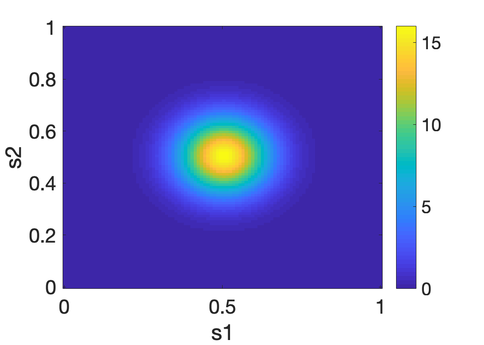
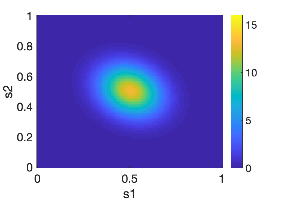
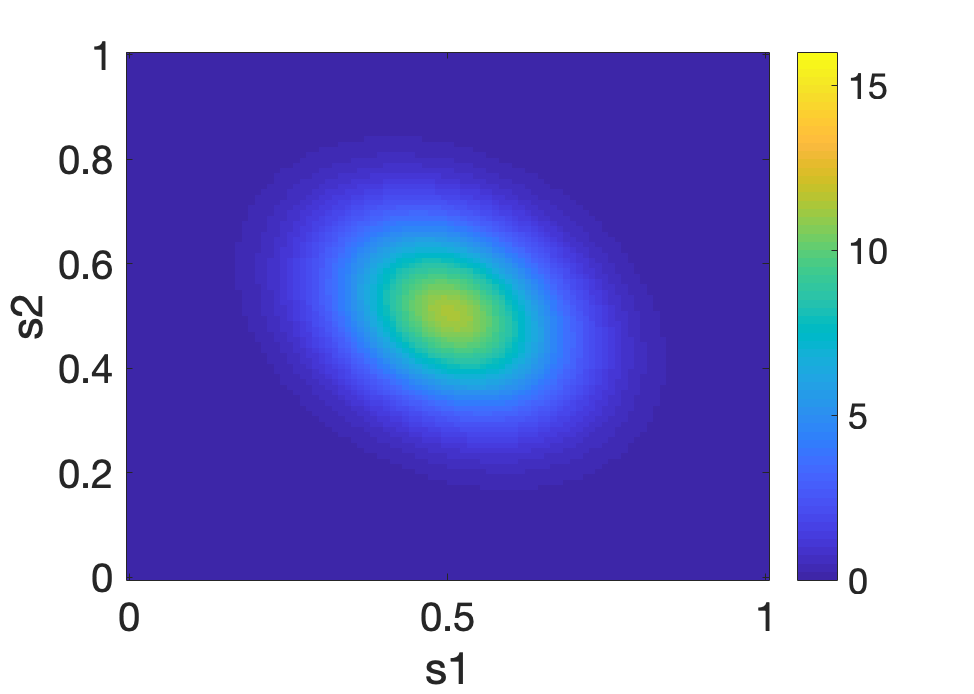
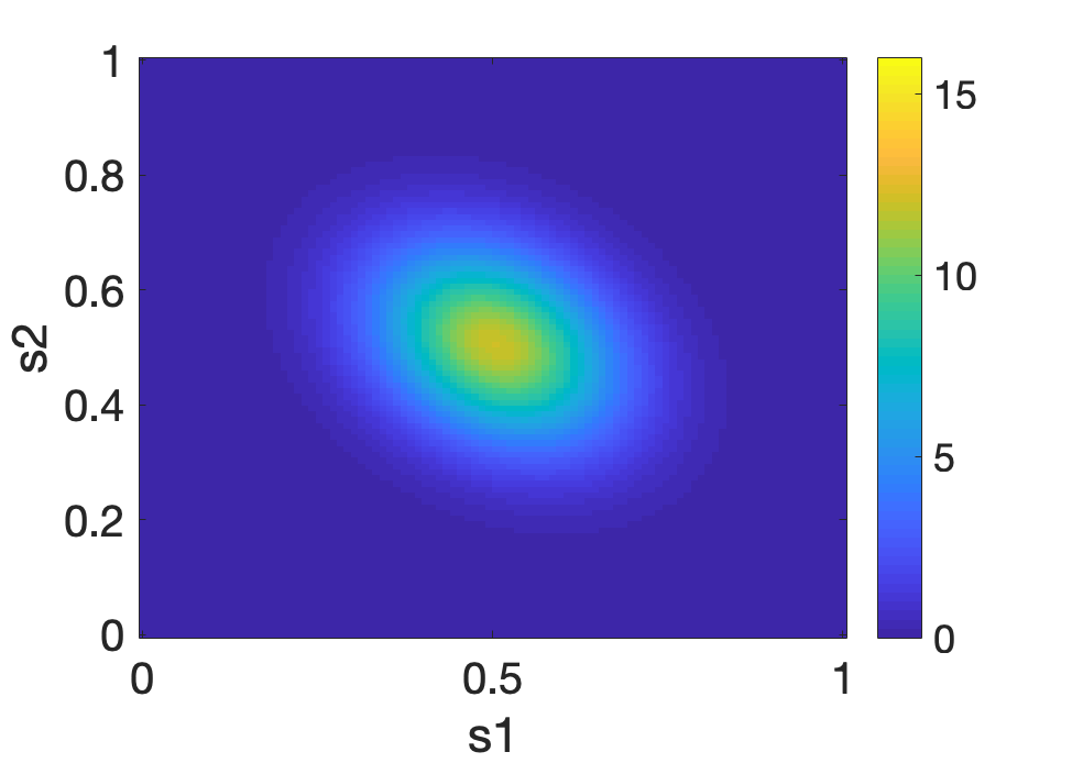
Figure 11: Extrapolation by fitting the global model for two-dimensional distributions when $n=2$. The top panels are heat maps for the distributions $(0,N((5,5),[1\quad 0;0\quad 1]))$ and $(1,N((5,5),[1.25\quad-0.25;-0.25\quad 1.25]))$, corresponding to the distributions at $x=0$ and $x=1$. The bottom left panel displays the global extrapolation at $x=1.5$ and the bottom right is the true extrapolation.

References

• Agueh and Carlier (2011) Agueh, M. and Carlier, G. (2011). Barycenters in the Wasserstein space. SIAM Journal on Mathematical Analysis 43 904–924.
• Ahidar-Coutrix et al. (2019) Ahidar-Coutrix, A., Le Gouic, T. and Paris, Q. (2019). Convergence rates for empirical barycenters in metric spaces: curvature, convexity and extendable geodesics. Probability Theory and Related Fields 1–46.
• Álvarez-Esteban et al. (2016) Álvarez-Esteban, P. C., Del Barrio, E., Cuesta-Albertos, J. and Matrán, C. (2016). A fixed-point approach to barycenters in Wasserstein space. Journal of Mathematical Analysis and Applications 441 744–762.
• Ambrosio et al. (2008) Ambrosio, L., Gigli, N. and Savaré, G. (2008). Gradient Flows in Metric Spaces and in the Space of Probability Measures. Springer Science & Business Media.
• Anderes et al. (2016) Anderes, E., Borgwardt, S. and Miller, J. (2016). Discrete Wasserstein barycenters: optimal transport for discrete data. Mathematical Methods of Operations Research 84 389–409.
• Bigot (2019) Bigot, J. (2019). Statistical data analysis in the Wasserstein space. arXiv:1907.08417 .
• Bigot et al. (2018) Bigot, J., Cazelles, E. and Papadakis, N. (2018). Data-driven regularization of Wasserstein barycenters with an application to multivariate density registration. arXiv preprint arXiv:1804.08962 .
• Bigot et al. (2019) Bigot, J., Cazelles, E. and Papadakis, N. (2019). Penalization of barycenters in the Wasserstein space. SIAM Journal on Mathematical Analysis 51 2261–2285.
• Bigot et al. (2017) Bigot, J., Gouet, R., Klein, T. and López, A. (2017). Geodesic PCA in the Wasserstein space by convex PCA. Annales de l’Institut Henri Poincaré B: Probability and Statistics 53 1–26.
• Boissard et al. (2015) Boissard, E., Le Gouic, T. and Loubes, J.-M. (2015). Distribution’s template estimate with Wasserstein metrics. Bernoulli 21 740–759.
• Buja et al. (2019a) Buja, A., Brown, L., Berk, R., George, E., Pitkin, E., Traskin, M., Zhang, K. and Zhao, L. (2019a). Models as approximations I: Consequences illustrated with linear regression. Statistical Science 34 523–544.
• Buja et al. (2019b) Buja, A., Brown, L., Kuchibhotla, A. K., Berk, R., George, E. and Zhao, L. (2019b). Models as approximations II: A model-free theory of parametric regression. Statistical Science 34 545–565.
• Burago et al. (2001) Burago, D., Burago, Y. and Ivanov, S. (2001). A Course in Metric Geometry. American Mathematical Society, Providence, RI.
• Buttazzo et al. (2012) Buttazzo, G., De Pascale, L. and Gori-Giorgi, P. (2012). Optimal-transport formulation of electronic density-functional theory. Physical Review A 85 062502.
• Carlier and Ekeland (2010) Carlier, G. and Ekeland, I. (2010). Matching for teams. Economic Theory 42 397–418.
• Chen et al. (2020) Chen, Y., Lin, Z. and Müller, H.-G. (2020). Wasserstein regression. arXiv:2006.09660 .
• Cuturi (2013) Cuturi, M. (2013). Sinkhorn distances: Lightspeed computation of optimal transport. In Advances in neural information processing systems.
• Cuturi and Doucet (2014) Cuturi, M. and Doucet, A. (2014). Fast computation of Wasserstein barycenters. In International Conference on Machine Learning, vol. 32.
• Cuturi and Peyré (2016) Cuturi, M. and Peyré, G. (2016). A smoothed dual approach for variational Wasserstein problems. SIAM Journal on Imaging Sciences 9 320–343.
• del Barrio and Loubes (2020) del Barrio, E. and Loubes, J.-M. (2020). The statistical effect of entropic regularization in optimal transportation. arXiv preprint arXiv:2006.05199 .
• Dvurechenskii et al. (2018) Dvurechenskii, P., Dvinskikh, D., Gasnikov, A., Uribe, C. and Nedich, A. (2018). Decentralize and randomize: Faster algorithm for Wasserstein barycenters. In Advances in Neural Information Processing Systems.
• Fréchet (1948) Fréchet, M. (1948). Les éléments aléatoires de nature quelconque dans un espace distancié. Annales de l‘Institut Henri Poincaré 10 215–310.
• Frogner et al. (2015) Frogner, C., Zhang, C., Mobahi, H., Araya, M. and Poggio, T. A. (2015). Learning with a Wasserstein loss. In Advances in Neural Information Processing Systems.
• Genevay et al. (2018) Genevay, A., Peyré, G. and Cuturi, M. (2018). Learning generative models with sinkhorn divergences. In International Conference on Artificial Intelligence and Statistics.
• Gibbs and Su (2002) Gibbs, A. L. and Su, F. E. (2002). On choosing and bounding probability metrics. International Statistical Review 70 419–435.
• Horvath and Kokoszka (2012) Horvath, L. and Kokoszka, P. (2012). Inference for Functional Data with Applications. Springer, New York.
• Huber (2004) Huber, P. J. (2004). Robust statistics, vol. 523. John Wiley & Sons.
• Janati et al. (2020) Janati, H., Cuturi, M. and Gramfort, A. (2020). Debiased Sinkhorn barycenters. arXiv preprint arXiv:2006.02575 .
• Le Gouic and Loubes (2017) Le Gouic, T. and Loubes, J.-M. (2017). Existence and consistency of Wasserstein barycenters. Probability Theory and Related Fields 168 901–917.
• McCann (1997) McCann, R. J. (1997). A convexity principle for interacting gases. Advances in Mathematics 128 153–179.
• Monge (1781) Monge, G. (1781). Mémoire sur la théorie des déblais et des remblais. Histoire de l’Académie Royale des Sciences de Paris .
• Neumayer and Steidl (2020) Neumayer, S. and Steidl, G. (2020). From optimal transport to discrepancy. arXiv preprint arXiv:2002.01189 .
• Panaretos and Zemel (2019) Panaretos, V. M. and Zemel, Y. (2019). Statistical aspects of Wasserstein distances. Annual Review of Statistics and its Application 6 405–431.
• Petersen and Müller (2016) Petersen, A. and Müller, H.-G. (2016). Functional data analysis for density functions by transformation to a Hilbert space. Annals of Statistics 44 183–218.
• Petersen and Müller (2019) Petersen, A. and Müller, H.-G. (2019). Fréchet regression for random objects with Euclidean predictors. The Annals of Statistics 47 691–719.
• Peyré (2015) Peyré, G. (2015). Entropic approximation of Wasserstein gradient flows. SIAM Journal on Imaging Sciences 8 2323–2351.
• Peyré and Cuturi (2019) Peyré, G. and Cuturi, M. (2019). Computational optimal transport: With applications to data science. Foundations and Trends in Machine Learning 11 355–607.
• Rabin et al. (2011) Rabin, J., Peyré, G., Delon, J. and Bernot, M. (2011). Wasserstein barycenter and its application to texture mixing. In International Conference on Scale Space and Variational Methods in Computer Vision. Springer.
• Rubner et al. (2000) Rubner, Y., Tomasi, C. and Guibas, L. J. (2000). The earth mover’s distance as a metric for image retrieval. International Journal of Computer Vision 40 99–121.
• Sheather and Jones (1991) Sheather, S. J. and Jones, M. C. (1991). A reliable data-based bandwidth selection method for kernel density estimation. Journal of the Royal Statistical Society: Series B (Methodological) 53 683–690.
• van der Vaart and Wellner (1996) van der Vaart, A. and Wellner, J. (1996). Weak Convergence and Empirical Processes with Applications to Statistics. Springer.
• Villani (2008) Villani, C. (2008). Optimal transport: Old and New, vol. 338. Springer Science & Business Media.
• Wang et al. (2016) Wang, J.-L., Chiou, J.-M. and Müller, H.-G. (2016). Functional data analysis. Annual Review of Statistics and its Application 3 257–295.