Integrated shape-sensitive functional metrics

Abstract

This paper develops a new integrated ball (pseudo)metric which provides an intermediary between a chosen starting (pseudo)metric $d$ and the $L_{p}$ distance in general function spaces. Selecting $d$ as the Hausdorff or Fréchet distances, we introduce integrated shape-sensitive versions of these supremum-based metrics. The new metrics allow for finer analyses in functional settings, not attainable applying the non-integrated versions directly. Moreover, convergent discrete approximations make computations feasible in practice.

1 Introduction

Measuring the shape similarity or dissimilarity of functions has been a concurrent problem in many fields of research. In functional data analysis, the shape features often comprise the key modes of variance in the functional observations and comparison problems such as classification are common. This can be seen, for instance, in the functional depth literature, where recent advances have begun emphasizing shape features as the focal point of analysis. See, for example Sguera et al. [31], Claeskens et al. [13], Harris et al. [20] and Nagy et al. [27, 28] for recent approaches to shape-sensitive functional depths.

Similarly, attention has been devoted to developing metrics that are more sensitive to variations in shape. The use of such metrics has become commonplace in shape and pattern matching applications in machine learning and computer vision. See Huttenlocher et al. [21], Rucklidge [29], Yi and Camps [34], Veltkamp and Hagedoorn [33], De Carvalho et al. [16], Alt and Godau [2], Alt et al. [1], Brakatsoulas et al. [10], Aronov et al. [5] and Jiang et al. [22] for a wide variety of applications for such shape-sensitive metrics. Popular approaches include considering Hausdorff or Fréchet distances between the graphs of the functions. However, as both of these distances are based on a global supremum, they do not consider the local likeness of the graphs. Therefore, in the literature some attention has been devoted to developing averaged (i.e. integrated) versions of these distances.

Baddeley [6] developed an integrated alternative to the Hausdorff metric by substituting the supremum for an integral in an expression equivalent to the usual definition. A more direct approach was taken by Marron and Tsybakov [26] who proposed an error criterion for nonparametric curve estimation, where the features of the curves are matched “vertically” in value and “horizontally” in timing. Schütze et al. [30] proposed an averaged version of the Hausdorff distance by replacing the sup-inf in its definition with an $L_{p}$ mean. Vargas and Bogoya [32] and Bogoya et al. [8] further developed the notion to an integrated counterpart.

The integrated Fréchet distance was studied in Buchin [12] who considered several approaches for both a summed and an averaged Fréchet distance and analyzed their properties. Efrat et al. [17] developed a notion of dynamic time warping that can be seen as an integrated version of the Fréchet distance. Buchin et al. [11] considered the partial curve matching problem where the similarity of two curves was measured by the largest fraction of their lengths that could be matched within a certain Fréchet distance threshold.

Many of the approaches discussed above, however, do not satisfy the key properties of a metric. See for example Marron and Tsybakov [26], Maheshwari et al. [24], and the extensive analysis provided by Buchin [12] for more details. Specifically, in the case of integrated Fréchet distances, the triangle inequality fails for approaches considered previously.

Use of pseudometrics (also called semimetrics) in FDA has been shown to be of interest. See, for example, Aneiros et al. [3, 4], Cuevas [14] and Goia and Vieu [19]. In this paper, we generalize any pseudometric $d$ on a function space to a family of integrated ball pseudometrics $d^{\epsilon,p}$, obtained through local integration of $d$. The locality parameter $\epsilon$ allows to control the shape sensitivity of the pseudometric by balancing between $d$ (for $\epsilon\to\infty$) and the $L_{p}$ distance (for $\epsilon\to 0$). Furthermore, we show that $d^{\epsilon,p}$ is a pseudometric for any $\epsilon$. Convergence of suitable discretizations ensures that the integrated ball pseudometric can be computed in practice. When the integrated distance $d$ is a metric, then, under mild technical assumptions, the integrated version is a metric as well.

The theoretical results are derived for general (pseudo)metrics $d$. In a second part of this paper, we apply the integrated ball construction to the Hausdorff and Fréchet distances, $d_{H}$ and $d_{F}$, and provide their locally integrated counterparts, $d_{H}^{\epsilon,p}$ and $d_{F}^{\epsilon,p}$. We show important properties of the integrated ball Hausdorff and Fréchet distances and study their behavior in a variety of simulated outlier detection settings. The appeal of local distances in the functional context is illustrated in Figure 1, where examining local distances $d^{\epsilon,p}_{H}$ and $d^{\epsilon,p}_{F}$, $p=2$, $\epsilon\in[0,1]$, highlights shape-outlying curves. In this example, the compactness of the domain $[0,1]$ of the functional data allows to restrict $\epsilon$ to $[0,1]$.

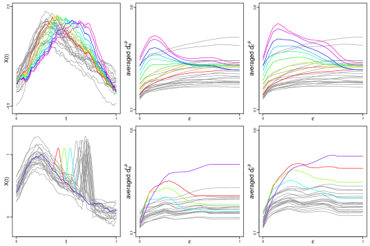
Figure 1: Motivating example showcasing the behavior of the integrated ball metrics $d_{H}^{\epsilon,p}$ and $d_{F}^{\epsilon,p}$ as a function of $\epsilon\in[0,1]$, $p=2$, in two simulated settings with shape-outlying curves (in color).

Figure 1 illustrates two models, drawn in gray in the left panels, with some contaminating observations drawn in color. On the top row, the outlying observations differ from the base model in phase, whereas on the bottom, three of the outliers have different timing of the sharp feature and one lacks it entirely. In the middle and right panels, the average $d_{H}^{\epsilon,p}$ and $d_{F}^{\epsilon,p}$ distances between the observations and each outlier are drawn in corresponding color, as a function of $\epsilon$, with the between-observation average distances drawn in light gray.

In the first model, global Hausdorff and Fréchet distances (corresponding to $\epsilon=1$) fail to properly separate the outliers from one another and from the rest of the observations. In the second model, the $L_{p}$ distance (for $\epsilon=0$) does not properly separate outlying curves and fares poorly in detecting them among the observations of the base model. Examining the curves $\epsilon\mapsto d_{H}^{\epsilon,p}$ and $\epsilon\mapsto d_{F}^{\epsilon,p}$ shows a different behavior for the outlying curves and allows proper separation on a wide range of values of the locality parameter $\epsilon$.

The rest of the paper is organized as follows: in Section 2 we introduce a general functional framework, under which we present the main contribution of the paper, the integrated ball (pseudo)metric $d^{\epsilon,p}$, and analyze its properties. We show that, under non-restrictive assumptions, $d^{\epsilon,p}$ is indeed a proper (pseudo)metric with many desirable properties. Furthermore, we provide an important convergence result for $d^{\epsilon,p}$ for discrete approximations of the functions, that ensures the feasibility of computations of the (pseudo)metric in practice. In Section 3, we formally introduce our two leading examples, the Hausdorff and Fréchet distances $d_{H}$ and $d_{F}$, and define their locally integrated counterparts, $d_{H}^{\epsilon,p}$ and $d_{F}^{\epsilon,p}$. We show that $d_{H}$ and $d_{F}$ satisfy our main assumptions and therefore $d_{H}^{\epsilon,p}$ and $d_{F}^{\epsilon,p}$ exhibit the properties stated in Section 2. In Section 4 we apply the integrated ball Hausdorff and Fréchet distances in simulated outlier detection settings, and study their behavior as a function of the locality parameter $\epsilon$. A discussion closes the paper.

2 Integrated ball metric

The framework considered in this paper is the following. Let $(\mathcal{X},d_{\mathcal{X}})$ and $(\mathcal{V},d_{\mathcal{V}})$ be two metric spaces. Throughout, we assume that $\mathcal{X}$ is a complete and a measure space with respect to a Borel probability measure $\mu$. Let $\mathcal{F}$ be a family of measurable and bounded functions $f:\mathcal{X}\to\mathcal{V}$. Recall that $f$ is bounded if the image $f(\mathcal{X})=\{f(x):x\in\mathcal{X}\}$ is a bounded subset of $\mathcal{V}$. As we consider bounded functions, $\mathcal{F}$ can be equipped with the usual supremum metric given by $\sup_{t\in\mathcal{X}}d_{\mathcal{V}}\left(f(t),g(t)\right).$ The curve associated with $f$ is denoted by $C_{f}$ and is defined as

$$C_{f}:\mathcal{X}\rightarrow\mathcal{X}\times\mathcal{V}:t\mapsto(t,f(t)).$$

The graph of $f$ is the image $G_{f}=C_{f}(\mathcal{X})\subset\mathcal{X}\times\mathcal{V}$.

For a function $f$, the restriction of $f$ to the set $A\subset\mathcal{X}$ is the function $f\raisebox{-2.15277pt}{$|$}_{A}:{A}\to\mathcal{V}$. In the sequel, by restriction of curve/graph of $f$ to $A$, we mean the curve/graph associated with the restriction of $f$ to $A$. Let $B(t,r)=\{x\in\mathcal{X}:d_{\mathcal{X}}(x,t)\leq r\}\subset\mathcal{X}$ denote the closed ball of radius $r$ centered at $t$. The restriction $f\raisebox{-2.15277pt}{$|$}_{B(t,\epsilon)}$ will be written $f_{(t,\epsilon)}$ throughout.

In order to take into account shape-sensitive features that are not detected by classical “vertical” measures depending only on pointwise distances $d_{\mathcal{V}}(f(t),g(t))$ in the image space $\mathcal{V}$, we consider a general distance $d$ defined on $\mathcal{X}\times\mathcal{V}$. More precisely, we assume that $d$ is a pseudometric defined for subsets of $\mathcal{X}\times\mathcal{V}$ of the form

$$\mathcal{B}:=\{B(t,r)\times f(B(t,r)):\ t\in\mathcal{X},\ r>0,\ f\in\mathcal{F}\}.$$

Elements of $\mathcal{B}$ are graphs of functions restricted to closed balls.

Remark 2.1.

We stress that, while the underlying spaces $(\mathcal{X},d_{\mathcal{X}})$ and $(\mathcal{V},d_{\mathcal{V}})$ are metric, the distance $d$ that we use throughout is only required to be a pseudometric on the product space $\mathcal{X}\times\mathcal{V}$. Note also that care must be taken on the definition of $d$ when one considers which subsets of $\mathcal{X}\times\mathcal{V}$ are accounted for. Indeed, it might be that $d$ provides a pseudometric when restricted to a suitable class of subsets of $\mathcal{X}\times\mathcal{V}$ while it is not if one considers all possible subsets. An example is the Hausdorff distance which is a metric only if restricted to non-empty compact subsets of $\mathcal{X}\times\mathcal{V}$.

Note that assuming that $d$ is defined on sets in $\mathcal{X}\times\mathcal{V}$ is natural. While there exist many definitions computing distances between functions $f\in\mathcal{F}$ ($L_{p}$ distances) or curves $C_{f}$ (Fréchet distance), they all can be interpreted as (pseudo)metrics on subsets of $\mathcal{X}\times\mathcal{V}$ due to the bijective nature of the mappings $f\mapsto C_{f}$ and $f\mapsto G_{f}$. In the sequel, we will use the notation $d(f,g)$, $d(C_{f},C_{g})$ and $d(G_{f},G_{g})$ interchangeably.

The running example that is used throughout considers the set of continuous functions $\mathcal{F}=\mathcal{C}([0,1],\mathbb{R}^{m})=\{f:[0,1]\rightarrow\mathbb{R}^{m},\ f\textrm{ continuous}\}$. Euclidean distances are used on both $\mathcal{X}=[0,1]$ and on $\mathcal{V}=\mathbb{R}^{m}$ and the Lebesgue measure makes the compact interval $[0,1]$ a measure space. The canonical metric on $\mathcal{F}$ is induced by the supremum distance. Then the pseudometric $d$ can be induced by the Hausdorff or Fréchet distances, see Section 3.

2.1 Definition

We start with introducing a family of local versions of $d$, the integrated ball metrics, which involve integrating distances between restricted functions.

Definition 2.1 (Integrated ball metric).

Let $d$ be a pseudometric on subsets of $\mathcal{X}\times\mathcal{V}$ and let $\mu$ be a Borel probability measure on $\mathcal{X}$. For a given $\epsilon>0$ and $1\leq p\leq\infty$, define the integrated ball metric $d^{\epsilon,p}$ between $f,g\in\mathcal{F}$ as

$$d^{\epsilon,p}(f,g):=\begin{cases}\left(\int_{\mathcal{X}}d(f_{(t,\epsilon)},g_{(t,\epsilon)})^{p}d\mu(t)\right)^{\frac{1}{p}}&\textrm{ for }p<\infty,\\[5.69054pt] \sup_{t\in\mathcal{X}}d(f_{(t,\epsilon)},g_{(t,\epsilon)})&\textrm{ for }p=\infty.\end{cases}$$

Note that, provided the integrand is measurable, the integral in Definition 2.1 exists and takes value in $[0,\infty]$. The integrated ball metric provides a flexible approach to construct local distances between functions. The next section shows that the locality parameter $\epsilon$ allows to consider distances ranging from the $L_{p}$ distance (for $\epsilon=0$) to $d$ itself (for $\epsilon\rightarrow\infty$). Similarly, freedom on the choice in the order $p$ and in the measure $\mu$ provides flexibility towards different applications. One can emphasize specific regions of $\mathcal{X}$ through the measure $\mu$, or adjust penalization for large deviations in small regions of space through the choice of $p$.

2.2 General properties

We now examine the continuity properties of $d^{\epsilon,p}$ and the assumptions required to ensure it being a (pseudo)metric. Our assumptions are collected below.

Assumptions

1. For $\epsilon>0$ fixed, for each $t\in\mathcal{X}$ it holds $\mu(B(t,\epsilon))>0$.

2. There exists $K>0$ such that, for all $t\in\mathcal{X}$ and $\epsilon\geq 0$,

   $$d(f_{(t,\epsilon)},g_{(t,\epsilon)})\leq K\sup\limits_{x\in\mathcal{X}}\ d_{\mathcal{V}}(f(x),g(x)).$$

3. For any $t\in\mathcal{X}$, it holds $\lim_{\epsilon\to 0}d(f_{(t,\epsilon)},g_{(t,\epsilon)})=d_{\mathcal{V}}(f(t),g(t)).$

4. For any $t\in\mathcal{X}$ and for any sequence $\epsilon_{n}\rightarrow\epsilon$, it holds $d(f_{(t,\epsilon_{n})},f_{(t,\epsilon)})\rightarrow 0.$

5. For any $\epsilon>0$ and for any sequence $t_{n}\rightarrow t$, it holds $d(f_{(t_{n},\epsilon)},f_{(t,\epsilon)})\rightarrow 0.$

Assumptions (A1)–(A5) above are mild and merely technical. Assumption (A1) is required for identifiability of pointwise values of the functions in this general setting and is not even required if one considers functions as equivalence classes $\mu$-almost everywhere. (A2) is a regularity condition on $d$ that supposes that two functions $f$ and $g$ cannot be arbitrarily far if their images are close (as measured via $d_{\mathcal{V}}$). In the example of continuous functions, this translates to an assumption that diagonal distances between points in the graphs of functions are bounded by a multiple of the vertical distances between functions. At the same time, (A2) ensures that the dominated convergence theorem can be applied. In conjunction with (A2), assumption (A3) ensures that $\lim_{\epsilon\to 0}d^{\epsilon,p}$ is indeed the $L^{p}$ distance on $\mathcal{F}$. (A4) and (A5) are natural continuity assumptions on $d$. (A4) ensures continuity of $d^{\epsilon,p}$ in $\epsilon$, while (A5) ensures continuity of the integrand in $t$.

We now state the main result for this section.

Theorem 1.

For any pseudometric $d$ on $\mathcal{B}$, for $1\leq p\leq\infty$ and for $\epsilon>0$, the integrated ball construction $d^{\epsilon,p}$ produces a pseudometric. Furthermore, $d^{\epsilon,p}$ becomes a true metric if $\mu$ satisfies (A1) and $d$ is, for any $t\in\mathcal{X}$, a metric on $\{B(t,\epsilon)\times f(B(t,\epsilon)):f\in\mathcal{F}\}$. Moreover, for any $f,g\in\mathcal{F}$, the following holds.

• Under (A2) is the map $d^{\epsilon,p}(\cdot,f)\equiv d^{\epsilon,p}(f,\cdot):\mathcal{F}\to[0,\infty]$ continuous.

• Under (A2) and assuming that $\mathcal{X}$ is bounded, $\lim_{\epsilon\rightarrow\infty}d^{\epsilon,p}(f,g)=d(f,g).$

• Under (A2) and (A3),

  $$\lim_{\epsilon\rightarrow 0}d^{\epsilon,p}(f,g)=\begin{cases}\left(\int_{\mathcal{X}}d_{\mathcal{V}}(f(t),g(t))^{p}d\mu(t)\right)^{\frac{1}{p}}&\textrm{for }1\leq p<\infty,\\[5.69054pt] \sup_{t\in\mathcal{X}}d_{\mathcal{V}}(f(t),g(t))&\textrm{for }p=\infty,\end{cases}$$

  that is, $d^{\epsilon,p}(f,g)$ converges to the $L_{p}$ distance on $\mathcal{F}$ as $\epsilon\to 0$.

• Under (A2) and (A4) the mapping $d^{\,\cdot\,,p}:[0,\infty)\rightarrow\mathbb{R}:\epsilon\mapsto d^{\epsilon,p}(f,g)$ is continuous.

We show in Section 3 that the Hausdorff and Fréchet distances satisfy (A1)–(A5) and consequently, Theorems 1 and 2 (below) are applicable. The integrated ball distance construction appears to be the first instance of a local version of the Fréchet distance that provides a continuous metric. This is also the case for the Hausdorff distance in the context of functional data.

Remark 2.2.

The boundedness assumption on $\mathcal{X}$ is only a sufficient condition for $(ii)$ of Theorem 1. Its proof shows that the statement remains valid more generally provided that $d(f_{(t,\epsilon)},g_{(t,\epsilon)})\to d(f,g)$ as $\epsilon\to\infty$, under further technical assumptions.

Proof of Theorem 1.

We prove the statements one by one and divide the proof into four steps.

Step 1a: $d^{\epsilon,p}$ is a pseudometric.
Since $d$ is a pseudometric on $\mathcal{B}$ and $f_{(t,\epsilon)},g_{(t,\epsilon)}\in\mathcal{B}$ for every $t\in\mathcal{X}$ and $\epsilon>0$, it follows trivially that $d^{\epsilon,p}(f,g)$ is symmetric, non-negative, and satisfies $d^{\epsilon,p}(f,f)=0$ for all $f\in\mathcal{F}$. In order to prove the triangle inequality for $d^{\epsilon,p}$, we observe from the triangle inequality for $d(f_{(t,\epsilon)},g_{(t,\epsilon)})$ that, for all $t\in\mathcal{X},\epsilon>0$, and $h\in\mathcal{F}$, we have

$$d(f_{(t,\epsilon)},g_{(t,\epsilon)})\leq d(f_{(t,\epsilon)},h_{(t,\epsilon)})+d(h_{(t,\epsilon)},g_{(t,\epsilon)}).$$

The claim for $p=1$ now follows by integration, and the general case $p>1$ from Minkowski’s inequality. This verifies the triangle inequality, and hence $d^{\epsilon,p}$ is a pseudometric.

Step 1b: $d^{\epsilon,p}$ is a metric.
Under the further assumption (A1) and the hypothesis that $d$ is a metric, suppose that $d^{\epsilon,p}(f,g)=0$, i.e.

$$\int_{\mathcal{X}}d(f_{(t,\epsilon)},g_{(t,\epsilon)})^{p}d\mu(t)=0.$$

It follows that

$$d(f_{(t,\epsilon)},g_{(t,\epsilon)})=0\hskip 14.22636pt\text{for }\mu-\text{almost every }t\in\mathcal{X},$$

and since $d$ is a metric on $\left\{B(t,\epsilon)\times f(B(t,\epsilon))\colon f\in\mathcal{F}\right\}$ for every $t\in\mathcal{X}$, we have

$$f(s)=g(s),\quad\forall s\in{B(t,\epsilon)}$$

for $\mu$-a.e. $t\in\mathcal{X}$. Let $A$ be the set of points $t$ satisfying the last formula. It holds $\mu(A^{c})=0$. This implies that $f(s)=g(s)$ for all $s\in\mathcal{X}$. Indeed, if that was not the case, then there exists $s$ such that $B(s,\epsilon)\subset A^{c}$, which contradicts (A1). This concludes step 1.

Step 2: Proof of statement (i).
For simplicity of notation, we prove only the case $p=1$, while the general case can be proved similarly. Using (A2), we get

$$d^{\epsilon,p}(f,g)=\int_{\mathcal{X}}d(f_{(t,\epsilon)},g_{(t,\epsilon)})d\mu(t)\leq K\sup_{s\in\mathcal{X}}d_{\mathcal{V}}(f(s),g(s)).$$

Now, let $f_{n}$ be a sequence of functions such that $\sup_{t\in\mathcal{X}}d_{\mathcal{V}}(f_{n}(t),f(t))\to 0$ as $n\rightarrow\infty$. Then, by the reverse triangle inequality, it holds that

$$|d^{\epsilon,p}(f_{n},g)-d^{\epsilon,p}(f,g)|\leq d^{\epsilon,p}(f,f_{n})\leq K\sup_{s\in\mathcal{X}}d_{\mathcal{V}}(f(s),f_{n}(s))\rightarrow 0.$$

The continuity in $g$ can be proved similarly, concluding step 2.

Step 3: Proof of statements (ii) and (iii).
By observing that (A2) allows us to use the dominated convergence theorem, statement (iii) follows directly from (A3). Similarly for statement (ii), boundedness of $\mathcal{X}$ gives $d(f_{(t,\epsilon)},g_{(t,\epsilon)})=d(f\raisebox{-2.15277pt}{$|$}_{\mathcal{X}},g\raisebox{-2.15277pt}{$|$}_{\mathcal{X}})=d(f,g)$ for $\epsilon$ large enough, from which the claim follows trivially.

Step 4: Proof of statement (iv).
Let $t$ be fixed. By the reverse triangle inequality we get

$$\left|d(f_{(t,\epsilon)},g_{(t,\epsilon+\delta)})-d(f_{(t,\epsilon+\delta)},g_{(t,\epsilon+\delta)})\right|\leq d(f_{(t,\epsilon+\delta)},f_{(t,\epsilon)}).$$

Treating $g$ similarly by symmetry, we get

$$\left|d(f_{(t,\epsilon+\delta)},g_{(t,\epsilon+\delta)})-d(f_{(t,\epsilon)},g_{(t,\epsilon)})\right|\leq d(f_{(t,\epsilon+\delta)},f_{(t,\epsilon)})+d(g_{(t,\epsilon+\delta)},g_{(t,\epsilon)}).$$

The claim follows directly from (A4) by using the dominated convergence theorem. This concludes step 4 and the whole proof. ∎

2.3 Computation

In practice, functions are only observed on a discrete grid, so that it is impossible to compute the exact value of the integrated ball distance between two data points $f$ and $g$. In this section, we construct approximations $d^{\epsilon,p}_{n}(f,g)$ of $d^{\epsilon,p}(f,g)$ that are consistent in $n$.

More precisely, let $\mu_{n}$ be a sequence of probability measures converging weakly to $\mu$. Let $d_{n}$ be a sequence of pseudometrics, which, for any $f$ and $g$ provides a sequence $d_{n}(f_{(t,\epsilon)},g_{(t,\epsilon)})$ of approximations of $d(f_{(t,\epsilon)},g_{(t,\epsilon)})$. In the practical setting, $\mu_{n}$ corresponds to a discrete measure on the observational grid. The pseudometrics $d_{n}$ are discrete approximations of $d$ based on the observed data points. The practical construction of $d_{n}$ depends on the underlying $d$ and specific examples are deferred to Section 4.

The following result ensures the consistency of suitable discretizations in practice.

Theorem 2.

For $\epsilon>0$ and $1\leq p\leq\infty$, suppose that (A2) and (A5) hold, that $\mu_{n}$ converges weakly to $\mu$ and that, as $n\to\infty$,

$$\sup_{t\in\mathcal{X}}\left|d_{n}(f_{(t,\epsilon)},g_{(t,\epsilon)})-d(f_{(t,\epsilon)},g_{(t,\epsilon)})\right|\to 0.$$ (2.1)

Then, defining $d_{n}^{\epsilon,p}(f,g)$ as $d^{\epsilon,p}(f,g)$ with $\mu=\mu_{n}$ and $d=d_{n}$, it holds that

$$d_{n}^{\epsilon,p}(f,g)\to d^{\epsilon,p}(f,g).$$

Proof of Theorem 2.

We consider $p<\infty$; the case $p=\infty$ is trivial. We have

$$\left[d_{n}^{\epsilon,p}(f,g)\right]^{p}= \int_{\mathcal{X}}\Big{[}d_{n}\left(f_{(t,\epsilon)},g_{(t,\epsilon)}\right)^{p}-d\left(f_{(t,\epsilon)},g_{(t,\epsilon)}\right)^{p}\Big{]}d\mu_{n}(t)$$

$$\qquad+\int_{\mathcal{X}}d\left(f_{(t,\epsilon)},g_{(t,\epsilon)}\right)^{p}d\mu_{n}(t).$$

Using the arguments of step 4 in the proof of Theorem 1 together with (A5) shows that, for fixed $f,g\in\mathcal{F}$, the mapping $t\mapsto d(f_{(t,\epsilon)},g_{(t,\epsilon)})$ is continuous and, by (A2), bounded. Hence, by definition of weak convergence [7],

$$\int_{\mathcal{X}}d\left(f_{(t,\epsilon)},g_{(t,\epsilon)}\right)^{p}d\mu_{n}(t)\to\int_{\mathcal{X}}d\left(f_{(t,\epsilon)},g_{(t,\epsilon)}\right)^{p}d\mu(t).$$

Furthermore, by our assumption (2.1) it holds that

$$\left|\int_{\mathcal{X}}d_{n}\left(f_{(t,\epsilon)},g_{(t,\epsilon)}\right)^{p}\right. -d\left(f_{(t,\epsilon)},g_{(t,\epsilon)}\right)^{p}d\mu_{n}(t)\bigg{|}$$

$$\leq\ \sup_{t\in\mathcal{X}}\left|d_{n}\left(f_{(t,\epsilon)},g_{(t,\epsilon)}\right)^{p}-d\left(f_{(t,\epsilon)},g_{(t,\epsilon)}\right)^{p}\right|\to 0,$$

and hence $\left[d_{n}^{\epsilon,p}(f,g)\right]^{p}\to\left[d^{\epsilon,p}(f,g)\right]^{p}$ which concludes the proof. ∎

Remark 2.3.

The proof of Theorem 2 can be generalized to incorporate measurement errors in $f$ and $g$. More precisely, the proof holds under the assumption

$$\sup_{t\in\mathcal{X}}\left|d_{n}(f_{n,(t,\epsilon)},g_{n,(t,\epsilon)})-d(f_{(t,\epsilon)},g_{(t,\epsilon)})\right|\to 0,$$

where $f_{n}$ and $g_{n}$ are approximations of $f$ and $g$ with measurement errors.

3 Examples

In the following, we study the more specific examples of integrated Hausdorff and Fréchet distances. Let $(\mathcal{X},\mu)=([0,1],\lambda)$ with $\lambda$ the Lebesgue measure and let $(\mathcal{V},d_{\mathcal{V}})=(\mathbb{R}^{m},d_{\mathcal{V}})$ with $d_{\mathcal{V}}$ the Euclidean distance. The definitions of Hausdorff and Fréchet distances require the use of a metric between points on curves, i.e. on $[0,1]\times\mathbb{R}^{m}$. We endow this space with the usual $q$-metric

$$d_{C}((t,v),(s,w)):=\begin{cases}\left(|t-s|^{q}+d_{\mathcal{V}}(v,w)^{q}\right)^{\frac{1}{q}}&\textrm{for }1\leq q<\infty,\\[5.69054pt] \max\left\{|t-s|,d_{\mathcal{V}}(v,w)\right\}&\textrm{for }q=\infty.\end{cases}$$ (3.1)

Choosing $q=2$ leads to $d_{C}$ becoming the metric induced by the $L_{2}$ norm on $\mathbb{R}^{m+1}$. For the sake of simplicity, in the sequel we restrict to $\mathcal{C}([0,1],\mathbb{R}^{m})$, the space of continuous functions $[0,1]\to\mathbb{R}^{m}$. The continuity ensures compactness of $f([0,1])$. This in turn allows us to restrict our considerations to non-empty compact subsets of $[0,1]\times\mathbb{R}^{m}$, for which the Hausdorff distance is a metric.

Definition 2.1 allows to turn any distance defined on restricted functions to a local integrated version. We start by providing such a distance between restrictions in the Hausdorff case.

Definition 3.1 (Hausdorff for restrictions).

Let $f\raisebox{-2.15277pt}{$|$}_{A}$ and $g\raisebox{-2.15277pt}{$|$}_{B}$ be the restrictions of the functions $f,g\in\mathcal{C}([0,1],\mathbb{R}^{m})$ to sets $A$ and $B$, respectively. Then, the Hausdorff distance $d_{H}$ for the restrictions is given by

$$d_{H}(f\raisebox{-2.15277pt}{$|$}_{A},g\raisebox{-2.15277pt}{$|$}_{B}):=\max\{\sup_{t\in A}\inf_{s\in B}d_{C}(C_{f}(t),C_{g}(s)),\ \sup_{s\in B}\inf_{t\in A}d_{C}(C_{f}(t),C_{g}(s))\}.$$

The integrated version of the Hausdorff distance follows.

Definition 3.2 (Integrated ball Hausdorff distance).

For a given $\epsilon\geq 0$, $1\leq p\leq\infty$ and $f,g\in\mathcal{C}([0,1],\mathbb{R}^{m})$, we define

$$d_{H}^{\epsilon,p}(f,g):=\begin{cases}\left(\int_{0}^{1}d_{H}(f_{(t,\epsilon)},g_{(t,\epsilon)})^{p}dt\right)^{\frac{1}{p}}&\textrm{for }1\leq p<\infty,\\[5.69054pt] \sup_{t\in[0,1]}d_{H}(f_{(t,\epsilon)},g_{(t,\epsilon)})&\textrm{for }p=\infty.\end{cases}$$

The Fréchet distance is defined using parametrizations of the curves of the functions. In the case of the Fréchet distance, care must therefore be taken in how the restrictions of the curves are handled. Recall the usual one-sided definition of the Fréchet distance from Buchin [12].

Definition 3.3 (One-sided Fréchet).

Let $\Phi$ be the set of all continuous monotonically increasing functions $\phi:[0,1]\mapsto[0,1]$ with $\phi(0)=0$ and $\phi(1)=1$. Then the one-sided Fréchet distance $d_{F}$ between the functions $f,g\in\mathcal{C}([0,1],\mathbb{R}^{m})$ is given by

$$d_{F}(f,g):=\inf_{\phi\in\Phi}\sup_{t\in[0,1]}d_{C}(C_{f}(t),C_{g}(\phi(t))).$$

In order to define a restricted version of this distance satisfying (A4) and (A5), one needs to compare functions defined on sets that do not necessarily overlap. To do so, the two domains are mapped to a shared interval, to ensure that both curve segments can be simultaneously traversed through a single parameter. Therefore, for $0\leq a\leq b\leq 1$, we denote

$$\tilde{f}_{[a,b]}:[0,1]\to\mathcal{V}:t\mapsto f(\theta_{[a,b]}(t)),$$

where $\theta_{[a,b]}:[0,1]\to[a,b]:t\mapsto a+(b-a)t$. This construction will be typically applied to function $f$ restricted to the interval $[a,b]\subset[0,1]$; the function $\tilde{f}_{[a,b]}$ is then a re-parametrization of $f\raisebox{-2.15277pt}{$|$}_{[a,b]}$ to the full domain $[0,1]$. Evidently, $\tilde{f}_{[0,1]}=f$. We also denote $\tilde{f}_{[a,b]}$ for $[a,b]=B(t,\epsilon)$ by the simpler $\tilde{f}_{(t,\epsilon)}$. This leads us to a slightly expanded definition of the Fréchet distance that is able to compare curve segments restricted to different intervals.

Definition 3.4 (One-sided Fréchet for restrictions).

Let $f\raisebox{-2.15277pt}{$|$}_{[a,b]}$ and $g\raisebox{-2.15277pt}{$|$}_{[c,d]}$ be the restrictions of the functions $f,g\in\mathcal{C}([0,1],\mathbb{R}^{m})$ to the respective subintervals $[a,b]$ and $[c,d]$ of $[0,1]$. Then, the one-sided Fréchet distance $d_{F}$ for restrictions is given by

$$d_{F}(f\raisebox{-2.15277pt}{$|$}_{[a,b]},g\raisebox{-2.15277pt}{$|$}_{[c,d]}):=d_{F}(\tilde{f}_{[a,b]},\tilde{g}_{[c,d]}).$$

In the case $[a,b]=[c,d]=[0,1]$, Definitions 3.4 and 3.3 coincide. With this definition of the Fréchet distance, the integrated ball Fréchet distance can now be defined.

Definition 3.5 (Integrated ball Fréchet distance).

For $\epsilon\geq 0$, $1\leq p\leq\infty$ and $f,g\in\mathcal{C}([0,1],\mathbb{R}^{m})$, define

$$d_{F}^{\epsilon,p}(f,g):=\begin{cases}\left(\int_{0}^{1}d_{F}(f_{(t,\epsilon)},g_{(t,\epsilon)})^{p}dt\right)^{\frac{1}{p}}&\textrm{for }1\leq p<\infty,\\[5.69054pt] \sup_{t\in[0,1]}d_{F}(f_{(t,\epsilon)},g_{(t,\epsilon)})&\textrm{for }p=\infty.\end{cases}$$

Both $d_{H}^{\epsilon,p}$ and $d_{F}^{\epsilon,p}$ inherit the properties of Theorems 1 and 2.

Theorem 3.

$d_{H}$ and $d_{F}$ are metrics that fulfill (A1)–(A5). Thus, for any $\epsilon\geq 0$ and $1\leq p\leq\infty$, $d_{H}^{\epsilon,p}$ and $d_{F}^{\epsilon,p}$ are metrics that satisfy all conclusions of Theorem 1 and Theorem 2.

Proof of Theorem 3.

We check that the Hausdorff and Fréchet distances, $d_{H}$ and $d_{F}$, satisfy assumptions (A1)–(A5) in our chosen setting. Then, the statements of Theorem 1 and Theorem 2 follow directly.

The Hausdorff case:
Note that the graphs of continuous functions $f\in\mathcal{C}([0,1],\mathbb{R}^{m})$ are compact sets in $[0,1]\times\mathbb{R}^{m}$. Therefore, the Hausdorff distance defines a metric for the restrictions of the graphs $f\raisebox{-2.15277pt}{$|$}_{A}$. In turn, $d_{H}^{\epsilon,p}$ is a metric.

(A1): Follows directly from our choice of $\mu$ being the Lebesgue measure.

(A2): We prove a stronger statement: for all $t\in[0,1]$ and $\epsilon>0$,

$$d_{H}(f_{(t,\epsilon)},g_{(t,\epsilon)})\leq\sup_{s\in{B(t,\epsilon)}}d_{\mathcal{V}}(f(s),g(s)).$$

From the definition of $d_{H}$ and using $d_{C}$ the $q$-metric (3.1), for any $a\in{B(t,\epsilon)}$, it holds that

$$\inf_{b\in{B(t,\epsilon)}}d_{C}(C_{f}(a),C_{g}(b))\leq d_{C}(C_{f}(a),C_{g}(a))=d_{\mathcal{V}}(f(a),g(a)),$$

from which it follows that

$$\sup_{a\in{B(t,\epsilon)}}\inf_{b\in{B(t,\epsilon)}}d_{C}(C_{f}(a),C_{g}(b))\leq\sup_{a\in{B(t,\epsilon)}}d_{\mathcal{V}}(f(a),g(a)).$$

The claim now follows by considering the definition of the Hausdorff distance and interchanging the roles of $f$ and $g$.

(A3): The first inequality in the proof of (A2) above, for continuous $f$ and $g$, implies that

$$\limsup_{\epsilon\rightarrow 0}d_{H}(f_{(t,\epsilon)},g_{(t,\epsilon)})\leq d_{\mathcal{V}}(f(t),g(t)).$$

For the lower bound, using Definition 3.1 and $d_{C}$ the $q$-metric, it holds that

$$d_{H}(f_{(t,\epsilon)},g_{(t,\epsilon)})\geq\inf_{s\in{B(t,\epsilon)}}d_{C}(C_{f}(t),C_{g}(s))=\inf_{s\in{B(t,\epsilon)}}\left[|t-s|^{q}+d_{\mathcal{V}}(f(t),g(s))^{q}\right]^{\frac{1}{q}}.$$

By continuity of $f$ and $g$, letting $\epsilon\rightarrow 0$, it follows that

$$\inf_{s\in{B(t,\epsilon)}}\left[|t-s|^{q}+d_{\mathcal{V}}(f(t),g(s))^{q}\right]^{\frac{1}{q}}\rightarrow d_{\mathcal{V}}(f(t),g(t)).$$

The proof for $q=\infty$ is analogous.

(A4) and (A5): Consider two restrictions $f_{(t_{1},\epsilon_{1})}$ and $f_{(t_{2},\epsilon_{2})}$ of a single function $f$. Obviously,

$$d_{H}(f_{(t_{1},\epsilon_{1})},f_{(t_{2},\epsilon_{2})})=\max \left\{\sup_{a\in B{(t_{1},\epsilon_{1})}\setminus B{(t_{2},\epsilon_{2})}}\inf_{b\in B{(t_{2},\epsilon_{2})}}d_{C}(C_{f}(a),C_{f}(b)),\right.$$

$$\left.\qquad\sup_{a\in B{(t_{2},\epsilon_{2})}\setminus B{(t_{1},\epsilon_{1})}}\inf_{b\in B{(t_{1},\epsilon_{1})}}d_{C}(C_{f}(a),C_{f}(b))\right\}.$$

From the continuity of $f$ we know that for each $\varepsilon_{f}>0$ there is $\delta>0$ such that $d_{C}(C_{f}(a),C_{f}(b))\leq\varepsilon_{f}$ when $|a-b|\leq\delta$.

Fix $t_{1}=t_{2}=t$, with $\epsilon_{1}=\epsilon_{n}$ and $\epsilon_{2}=\epsilon$. Suppose, w.l.o.g. that $\epsilon_{n}>\epsilon$. Then $B{(t,\epsilon)}\subset B{(t,\epsilon_{n})}$. Consider $a\in B{(t,\epsilon_{n})}\setminus B{(t,\epsilon)}$. There is a point $b\in B{(t,\epsilon)}$ such that $|a-b|\leq|\epsilon_{n}-\epsilon|$. For $n$ large enough, we have $|\epsilon_{n}-\epsilon|<\delta$ and consequently $d_{H}(f_{(t,\epsilon_{n})},f_{(t,\epsilon)})\leq\varepsilon_{f}$. This shows (A4).

Fix now $\epsilon_{1}=\epsilon_{2}=\epsilon$, with $t_{1}=t_{n}$ and $t_{2}=t$. If $a\in B{(t_{n},\epsilon)}\setminus B{(t,\epsilon)}$ or $a\in B{(t,\epsilon)}\setminus B{(t_{n},\epsilon)}$, there is $b$ from $B{(t,\epsilon)}$ or $B{(t_{n},\epsilon)}$, respectively, satisfying $|a-b|\leq|t_{n}-t|$. Again, if $n$ is chosen large enough so that $|t_{n}-t|<\delta$, the desirable inequality $d_{H}(f_{(t_{n},\epsilon)},f_{(t,\epsilon)})\leq\varepsilon_{f}$ follows. This shows (A5).

The Fréchet case:
Note that $d_{F}$ is a metric, and thus so is $d_{F}(f_{(t,\epsilon)},g_{(t,\epsilon)})$ for every $t$ and any $\epsilon$. In turn, $d_{F}^{\epsilon,p}$ is a metric.

(A1): The claim follows directly as for the Hausdorff distance.

(A2): Again, we prove a stronger statement: for all $t\in[0,1]$ and $\epsilon>0$,

$$d_{F}(f_{(t,\epsilon)},g_{(t,\epsilon)})\leq\sup_{s\in{B(t,\epsilon)}}d_{\mathcal{V}}(f(s),g(s)).$$

Denote by ${\tilde{C}_{f}}$ and $\tilde{C}_{g}$ the curves corresponding to $\tilde{f}_{(t,\epsilon)}$ and $\tilde{g}_{(t,\epsilon)}$, respectively (with the ball $B(t,\epsilon)$ properly restricted to $[0,1]$). The choice of $d_{C}$ to be the $q$-metric (3.1) yields

$$d_{F}(f_{(t,\epsilon)},g_{(t,\epsilon)}) =\inf\limits_{\phi\in\Phi}\sup\limits_{s\in[0,1]}d_{C}(\tilde{C}_{f}(s),\tilde{C}_{g}(\phi(s)))\leq\sup\limits_{s\in[0,1]}d_{C}(\tilde{C}_{f}(s),\tilde{C}_{g}(s))$$

$$=\sup\limits_{s\in[0,1]}d_{\mathcal{V}}(\tilde{f}_{(t,\epsilon)}(s),\tilde{g}_{(t,\epsilon)}(s))=\sup\limits_{s\in B(t,\epsilon)}d_{\mathcal{V}}(f(s),g(s)),$$

and the claim follows directly.

(A3): The reasoning in the proof of (A2) above, for continuous $f$ and $g$, implies that

$$\limsup_{\epsilon\rightarrow 0}d_{F}(f_{(t,\epsilon)},g_{(t,\epsilon)})\leq d_{\mathcal{V}}(f(t),g(t)).$$

For the lower bound, fix $t\in[0,1]$. By the continuity of both $f$ and $g$, for any $\eta>0$ there exists $\epsilon>0$ such that $\left|s-t\right|\leq\epsilon$ implies $d_{\mathcal{V}}(f(t),f(s))\leq\eta$ and $d_{\mathcal{V}}(g(t),g(s))\leq\eta$. For any $s_{1},s_{2}\in[0,1]$ with $\left|s_{1}-t\right|\leq\epsilon$ and $\left|s_{2}-t\right|\leq\epsilon$ we obtain

$$d_{\mathcal{V}}(f(t),g(t)) \leq d_{\mathcal{V}}(f(t),f(s_{1}))+d_{\mathcal{V}}(f(s_{1}),g(s_{2}))+d_{\mathcal{V}}(g(s_{2}),g(t))$$

$$\leq 2\,\eta+d_{\mathcal{V}}(f(s_{1}),g(s_{2})).$$

For any $s_{1},s_{2}\in B(t,\epsilon)$, we get that $d_{\mathcal{V}}(f(s_{1}),g(s_{2}))\geq d_{\mathcal{V}}(f(t),g(t))-2\,\eta$, meaning that when restricted to the ball $B(t,\epsilon)$, the graphs of the functions $f$ and $g$ are at least $(d_{\mathcal{V}}(f(t),g(t))-2\,\eta)$-separated. Definition 3.4 directly gives that $d_{F}(f_{(t,\epsilon)},g_{(t,\epsilon)})\geq d_{\mathcal{V}}(f(t),g(t))-2\,\eta$. Taking $\eta\to 0$, we obtain

$$\liminf_{\epsilon\rightarrow 0}d_{F}(f_{(t,\epsilon)},g_{(t,\epsilon)})\geq d_{\mathcal{V}}(f(t),g(t)),$$

which together with the bound for the upper limit yields the result.

(A4) and (A5): For any intervals $[a,b],[c,d]\subset[0,1]$ we can write for $s\in[0,1]$

$$\left|\theta_{[c,d]}(s)-\theta_{[a,b]}(s)\right|=\left|(c-a)(1-s)+(d-b)s\right|\leq\max\{|c-a|,|d-b|\}.$$

Consequently, for any $s\in[0,1]$, $\epsilon\geq 0$, and $\delta\geq 0$

$$|\theta_{{B(t,\epsilon)}}(s)-\theta_{{B(t,\epsilon+\delta)}}(s)|\leq\delta\quad\mbox{ and }\quad|\theta_{{B(t,\epsilon)}}(s)-\theta_{{B(t+\delta,\epsilon)}}(s)|\leq\delta.$$

By Definition 3.4 and the definition of the $q$-metric (3.1) it holds that

$$d_{F}(f_{(t,\epsilon)},f_{(t,\epsilon+\delta)}) =\inf_{\phi\in\Phi}\sup_{s\in[0,1]}d_{C}(\tilde{f}_{(t,\epsilon)}(s),\tilde{f}_{(t,\epsilon+\delta)}(\phi(s)))$$

$$\leq\sup_{s\in[0,1]}d_{C}(\tilde{f}_{(t,\epsilon)}(s),\tilde{f}_{(t,\epsilon+\delta)}(s))$$

$$=\sup_{s\in[0,1]}d_{\mathcal{V}}(f(\theta_{{B(t,\epsilon)}}(s)),f(\theta_{{B(t,\epsilon+\delta)}}(s)))\leq\varepsilon_{f}.$$

The last inequality uses our first derived bound and the continuity of $f$, which gives that $d_{\mathcal{V}}(f(s_{1}),f(s_{2}))\leq\varepsilon_{f}$ whenever $|s_{1}-s_{2}|\leq\delta$. The claim now follows by letting $\delta\rightarrow 0$, since in that case we may write $\varepsilon_{f}\to 0$. This concludes (A4). To prove (A5), one uses the same argument and the second inequality above. ∎

Remark 3.1.

As an interesting special case, consider $[0,1]\times\mathcal{V}$ equipped with the $L_{\infty}$ distance

$$d_{C}(C_{f}(t),C_{g}(s))=\max\{|t-s|,\|f(t)-g(s)\|_{\mathcal{V}}\},$$

where $\|\cdot\|_{\mathcal{V}}$ is a norm on $\mathcal{V}$. Then, the one-sided Fréchet distance is equivalent to the Skorokhod distance (see Billingsley [7]) between the curves $C_{f}$ and $C_{g}$ (see Majumdar and Prabhu [25]), and consequently $d_{F}^{\epsilon,p}$ yields an integrated ball version of the Skorokhod distance.

4 Simulated examples

Hausdorff and Fréchet distances are commonly used in pattern matching and outlier detection applications. In this section, we study the behavior of the associated integrated ball metrics in a range of simulated examples considered in the literature. The distances $d_{H}^{\epsilon,p}$ and $d_{F}^{\epsilon,p}$ are computed in four different settings: three models described in Dai et al. [15], together with an additional model designed in the spirit of the motivating example of Marron and Tsybakov [26]. Throughout this section, we use $p=2$.

Each of the models presents different types of outliers controlled by outlyingness parameters. For each outlier type, we study the behavior of $d_{H}^{\epsilon,p}$ and $d_{F}^{\epsilon,p}$ as a function of the locality parameter $\epsilon$, over a range of parameter combinations. The four outlier models are described below. In each model, $e_{X}(t)$ is a centered Gaussian process with covariance function $K(s,t)=\mathrm{cov}\{e_{X}(s),e_{X}(t)\}=\exp\{-|s-t|\}$.

Model 1 (Jump): The base model is $X(t)=4t+e_{X}(t),\ t\in[0,1]$. The outlier model is $Y(t)=4t+H_{1}\,\mathbb{I}_{\left\{t>0.7\right\}}+e_{X}(t)$, where $\mathbb{I}$ is the indicator function, and the parameter $H_{1}$, controlling the height of the jump, was chosen on a uniform grid in $[0,2]$.

Model 2 (Peak): The base model is the same as in Model 1. The outlier model is $Y(t)=4t+H_{2}\,\mathbb{I}_{\left\{0.5-W\leq t\leq 0.5+W\right\}}+e_{X}(t)$. The parameters $H_{2}\in[0.5,3]$ and $W\in[0,0.2]$, controlling the height and width of the peak (respectively), were chosen on uniform grids on their respective intervals.

Model 3 (Phase): The general model is $X(t)=S_{P}(t)+0.9\,e_{X}(t),\ t\in[0,1]$, where $S_{P}(t)$ is the function with a peak of height $6$ at $t=P$, generated by smoothing (using a Gaussian smoother) the piecewise linear function interpolating the points $(0,0)$, $(P,6)$ and $(1,0)$. For the base model, the peak is located at $P=0.3$. The outlier model is $Y(t)=S_{P}(t)+0.9\,e_{X}(t),\ t\in[0,1]$, where the peak location parameter $P$ was chosen from a uniform grid on $[0.3,0.7]$.

Model 4 (Feature misalignment): The general model is

$$X(t)=\mathbb{I}_{\left\{|t-T|>0.06\right\}}(S(t)+0.25\,e_{X}(t))+\mathbb{I}_{\left\{|t-T|\leq 0.06\right\}}L_{T,H}(t),$$

where $S(t)$ is the function with a peak of height $3$ generated by smoothing the piecewise linear function interpolating the points $(0,2)$, $(0.2,3)$ and $(1,0)$ and $L_{T,H}(t)$ is a piecewise linear function that generates a peak of height $H$ at $T$. The function $L_{T,H}(t)$ interpolates the points $(T-0.06,S(T-0.06)+0.25\,e_{X}(T-0.06))$, $(T,H)$ and $(T+0.06,S(T+0.06)+0.25\,e_{X}(T+0.06))$. For the base model, the peak times $T$ followed the uniform distribution on $[0.7,0.85]$ and peak heights $H$ followed the uniform distribution on $[3,4]$. For the outlier model, the peak height was $3.5$ and the peak times $T$ were chosen from a uniform grid on $[0.3,0.8]$.

For each model, we simulated $20$ realizations from a base model and added the outliers for different parameter combinations. For each of the outliers, we computed their average distances $d_{H}^{\epsilon,p}$ and $d_{F}^{\epsilon,p}$ to the observations of the base models, for $\epsilon\in[0,1]$. For comparison, we also computed the corresponding average distances $d_{H}^{\epsilon,p}$ and $d_{F}^{\epsilon,p}$ between the observations, without the presence of the contaminating outliers. Figure 2 displays the realizations, together with the average integrated ball Hausdorff and Fréchet distances as a function of $\epsilon$. For a cleaner comparison of the outlier types, the same realizations were used in Models $1$ and $2$ for the observations from the base model as well as the error function $e_{X}$ of the outlier.

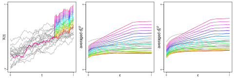
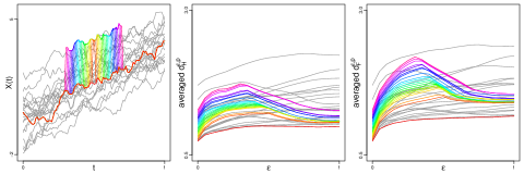
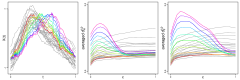
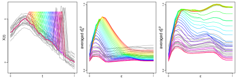
Figure 2: First column: $20$ i.i.d. realizations from Models $1-4$ (in rows) with contaminating curves displayed in color. Second and third columns: Averaged $d_{H}^{\epsilon,p}$ and $d_{F}^{\epsilon,p}$ distances (as functions of $\epsilon\in[0,1]$) between outliers and observations (in color) and between observations (in gray).

The integrated ball Hausdorff and Fréchet distances exhibit a range of interesting behaviors across the different models. Not only do the curves $\epsilon\mapsto d_{H}^{\epsilon,p}$ and $\epsilon\mapsto d_{F}^{\epsilon,p}$ associated with outliers allow to separate them from the non-contaminated observations, they also present strikingly different structures to those of the base model.

In Model 1 (jump outlier), the values of $d_{H}^{\epsilon,p}$ and $d_{F}^{\epsilon,p}$ grow steadily from the $L_{p}$ distance (at $\epsilon=0$) to the value of the corresponding global metric (at $\epsilon=1$). For both distances, this behavior is due to the outlying domain being included in a larger collection of balls in Definition 2.1, as the radius of the ball increases towards covering the entire domain. Furthermore, the outliers clearly display a different behavior from the base observations: the distances $d_{H}^{\epsilon,p}$ and $d_{F}^{\epsilon,p}$ initially increase and then reach a plateau, staying nearly constant at the global Hausdorff, resp. Fréchet, value.

Models $2$ and $3$ exhibit interesting peaked behavior. Initially, as $\epsilon$ grows, the outlying peak is included in a larger set of balls, increasing the value of the metric. However, as $\epsilon$ keeps growing, the local matching of the features becomes less strict, allowing the curves to be matched more diagonally.

In Model $2$, the values of $d_{H}^{\epsilon,p}$ and $d_{F}^{\epsilon,p}$ grow from the $L_{p}$ distance towards a pronounced peak that occurs between $\epsilon=0.2$ to $\epsilon=0.5$ (depending on the width of the peak), before settling down at a lower value of the corresponding global metric. When the level of the peak was not clearly above the highest observations of the base model, the global $d_{H}$ and $d_{F}$ both did a poor job at picking out the outlying functions. With suitable choices of $\epsilon$, the integrated ball versions were able to single out and separate the outliers much better than their global counterparts. With narrow peak widths, the $L_{p}$ distance also struggles to notice the outliers.

In Model $3$ the peaked behavior is extremely pronounced. As the scale of the $y$-axis is larger than that of the $x$-axis, it becomes less penalizing to match the curves horizontally rather than vertically. In this case, this behavior is very prominent, as the global versions of $d_{H}$ and $d_{F}$ measure the distances between the curves almost exclusively horizontally. This kind of behavior can be beneficial, for example in applications where the variation in phase is of lesser concern than the variation in amplitude. In Model 3, the integrated versions $d_{H}^{\epsilon,p}$ and $d_{F}^{\epsilon,p}$ allow for better control in the locality of this “feature matching” property.

In Models 2 and 3, the shapes of the integrated ball metric curves allow to discriminate immediately between outliers and noncontaminated curves: the outliers produce redescending distances as $\epsilon$ grows to $1$.

In Model $4$, the global Hausdorff distance fails to isolate the outliers, even when the timing of the sharp feature is extremely misplaced compared to the base model. As opposed to Model 3, the $L_{p}$ distances do not detect the outliers either, while the global Fréchet distance does. In both cases, however, the integrated ball versions exhibit the interesting peaked behavior, seen in Model $2$ and Model $3$ as well.

5 Discussion

This paper provides an integrated version of any pseudometric $d$. Naturally, the integrated version $d^{\epsilon,p}$ of $d$ inherits some properties of its underlying pseudometric $d$ as we illustrate in Theorems 1 and 2. An exhaustive study of the links between integrated and base metric is beyond the scope of this paper. We, however, provide a few avenues of research that might prove fruitful in the future.

Using pseudometrics in FDA is of interest in many statistical problems. Section 4 illustrates this in an outlier detection setting. Of course, such metrics are of interest in other problems, such as nonparametric regression (where metrics can be used in functional kernel regression), clustering, and classification. See, for example, the review papers Aneiros et al. [3, 4], Cuevas [14] and Goia and Vieu [19].

In the regression setting, asymptotic analysis requires studying small ball probabilities (SBPs). Very little is known for Fréchet and Hausdorff distances in that respect. Such analyses are therefore promising, yet technically challenging prospects for future research. In a more general framework, one might be interested in deriving functional SBPs based on corresponding results for the underlying (pseudo)metric $d$. For existing results on SBPs in FDA or the setting of Gaussian processes, see Bongiorno and Goia [9], Ferraty and Vieu [18] and Li and Shao [23].

Finally, the results derived in this paper deal with a general pseudometric $d$. In practical applications, one might wish to select $d$ adaptively to the problem at hand. While there is no universal optimal selection procedure for $d$, crossvalidation (choosing $d$ in a given set of pseudometrics) could be applied in selected applications, such as classification or regression. Naturally, regardless of the choice of $d$, crossvalidation can be conducted on $\epsilon$ and/or $p$ as well.

References

- Alt et al. [2003] H. Alt, A. Efrat, G. Rote, C. Wenk, Matching planar maps, Journal of Algorithms 49 (2003) 262–283.
- Alt and Godau [????] H. Alt, M. Godau, Measuring the resemblance of polygonal curves, in: Proceedings of the Eighth Annual Symposium on Computational Geometry, 1992, pp. 102–109.
- Aneiros et al. [2019a] G. Aneiros, R. Cao, R. Fraiman, P. Vieu, Editorial for the special issue on functional data analysis and related topics, Journal of Multivariate Analysis 170 (2019a) 1–2.
- Aneiros et al. [2019b] G. Aneiros, R. Cao, P. Vieu, Editorial for the special issue on functional data analysis and related topics, Computational Statistics 34 (2019b) 447–450.
- Aronov et al. [2006] B. Aronov, S. Har-Peled, C. Knauer, Y. Wang, C. Wenk, Fréchet distance for curves, revisited, in: European Symposium on Algorithms, Springer, Berlin, Heidelberg, 2006, pp. 52–63.
- Baddeley [1992] A. J. Baddeley, Errors in binary images and an version of the Hausdorff metric, Nieuw Archief voor Wiskunde 10 (1992) 157–183.
- Billingsley [1999] P. Billingsley, Convergence of probability measures, Wiley Series in Probability and Statistics: Probability and Statistics, John Wiley Sons, Inc., New York, second edition, 1999. A Wiley-Interscience Publication.
- Bogoya et al. [2018] J. M. Bogoya, A. Vargas, O. Cuate, O. Schütze, A -averaged Hausdorff distance for arbitrary measurable sets, Mathematical and Computational Applications 23 (2018) 51.
- Bongiorno and Goia [2017] E. G. Bongiorno, A. Goia, Some insights about the small ball probability factorization for Hilbert random elements, Statistica Sinica 27 (2017) 1949–1965.
- Brakatsoulas et al. [????] S. Brakatsoulas, D. Pfoser, R. Salas, C. Wenk, On map-matching vehicle tracking data, in: Proceedings of the 31st International Conference on Very Large Data Bases, 2005, pp. 853–864.
- Buchin et al. [2009] K. Buchin, M. Buchin, Y. Wang, Exact algorithms for partial curve matching via the Fréchet distance, in: Proceedings of the Twentieth Annual ACM-SIAM Symposium on Discrete Algorithms, Society for Industrial and Applied Mathematics, 2009, pp. 645–654.
- Buchin [2007] M. E. Buchin, On the computability of the Fréchet distance between triangulated surfaces, Ph.D. thesis, Freie Universität Berlin, Germany, 2007.
- Claeskens et al. [2014] G. Claeskens, M. Hubert, L. Slaets, K. Vakili, Multivariate functional halfspace depth, Journal of the American Statistical Association 109 (2014) 411–423.
- Cuevas [2014] A. Cuevas, A partial overview of the theory of statistics with functional data, Journal of Statistical Planning and Inference 147 (2014) 1–23.
- Dai et al. [2020] W. Dai, T. Mrkvička, Y. Sun, M. G. Genton, Functional outlier detection and taxonomy by sequential transformations, Computational Statistics & Data Analysis 149 (2020) 106960.
- De Carvalho et al. [2006] F. D. A. De Carvalho, R. M. de Souza, M. Chavent, Y. Lechevallier, Adaptive Hausdorff distances and dynamic clustering of symbolic interval data, Pattern Recognition Letters 27 (2006) 167–179.
- Efrat et al. [2007] A. Efrat, Q. Fan, S. Venkatasubramanian, Curve matching, time warping, and light fields: New algorithms for computing similarity between curves, Journal of Mathematical Imaging and Vision 27 (2007) 203–216.
- Ferraty and Vieu [2006] F. Ferraty, P. Vieu, Nonparametric functional data analysis: Theory and practice, Springer Science & Business Media, 2006.
- Goia and Vieu [2016] A. Goia, P. Vieu, An introduction to recent advances in high/infinite dimensional statistics [Editorial], Journal of Multivariate Analysis 146 (2016) 1–6.
- Harris et al. [2020] T. Harris, J. D. Tucker, B. Li, L. Shand, Elastic depths for detecting shape anomalies in functional data, 2020. Technometrics, To appear.
- Huttenlocher et al. [1993] D. P. Huttenlocher, G. A. Klanderman, W. J. Rucklidge, Comparing images using the Hausdorff distance, IEEE Transactions on Pattern Analysis and Machine Intelligence 15 (1993) 850–863.
- Jiang et al. [2008] M. Jiang, Y. Xu, B. Zhu, Protein structure–structure alignment with discrete Fréchet distance, Journal of Bioinformatics and Computational Biology 6 (2008) 51–64.
- Li and Shao [2001] W. V. Li, Q. M. Shao, Gaussian processes: inequalities, small ball probabilities and applications, Handbook of Statistics 19 (2001) 533–597.
- Maheshwari et al. [2018] A. Maheshwari, J. R. Sack, C. Scheffer, Approximating the integral Fréchet distance, Computational Geometry 70 (2018) 13–30.
- Majumdar and Prabhu [????] R. Majumdar, V. S. Prabhu, Computing the Skorokhod distance between polygonal traces, in: Proceedings of the 18th International Conference on Hybrid Systems: Computation and Control, 2015, pp. 199–208.
- Marron and Tsybakov [1995] J. S. Marron, A. B. Tsybakov, Visual error criteria for qualitative smoothing, Journal of the American Statistical Association 90 (1995) 499–507.
- Nagy et al. [2017] S. Nagy, I. Gijbels, D. Hlubinka, Depth-based recognition of shape outlying functions, Journal of Computational and Graphical Statistics 26 (2017) 883–893.
- Nagy et al. [2021] S. Nagy, S. Helander, G. Van Bever, L. Viitasaari, P. Ilmonen, Flexible integrated functional depths, Bernoulli 27 (2021) 673–701.
- Rucklidge [1997] W. J. Rucklidge, Efficiently locating objects using the Hausdorff distance, International Journal of Computer Vision 24 (1997) 251–270.
- Schütze et al. [2012] O. Schütze, X. Esquivel, A. Lara, C. A. C. Coello, Using the averaged Hausdorff distance as a performance measure in evolutionary multiobjective optimization, IEEE Transactions on Evolutionary Computation 16 (2012) 504–522.
- Sguera et al. [2014] C. Sguera, P. Galeano, R. Lillo, Spatial depth-based classification for functional data, TEST 23 (2014) 725–750.
- Vargas and Bogoya [2018] A. Vargas, J. M. Bogoya, A generalization of the averaged Hausdorff distance, Computación y Sistemas 22 (2018) 331–345.
- Veltkamp and Hagedoorn [2001] R. C. Veltkamp, M. Hagedoorn, State of the art in shape matching, in: Principles of Visual Information Retrieval. Advances in Pattern Recognition., Springer, London, 2001, pp. 87–119.
- Yi and Camps [1999] X. Yi, O. I. Camps, Line-based recognition using a multidimensional Hausdorff distance, IEEE Transactions on Pattern Analysis and Machine Intelligence 21 (1999) 901–916.