VolcanoML: Speeding up End-to-End AutoML via
Scalable Search Space Decomposition

Abstract.

End-to-end AutoML has attracted intensive interests from both academia and industry, which automatically searches for ML pipelines in a space induced by feature engineering, algorithm/model selection, and hyper-parameter tuning. Existing AutoML systems, however, suffer from scalability issues when applying to application domains with large, high-dimensional search spaces. We present VolcanoML, a scalable and extensible framework that facilitates systematic exploration of large AutoML search spaces. VolcanoML introduces and implements basic building blocks that decompose a large search space into smaller ones, and allows users to utilize these building blocks to compose an execution plan for the AutoML problem at hand. VolcanoML further supports a Volcano-style execution model – akin to the one supported by modern database systems – to execute the plan constructed. Our evaluation demonstrates that, not only does VolcanoML raise the level of expressiveness for search space decomposition in AutoML, it also leads to actual findings of decomposition strategies that are significantly more efficient than the ones employed by state-of-the-art AutoML systems such as auto-sklearn.

PVLDB Reference Format:
Yang Li, Yu Shen, Wentao Zhang, Jiawei Jiang, Bolin Ding, Yaliang Li, Jingren Zhou, Zhi Yang, Wentao Wu, Ce Zhang, and Bin Cui. VolcanoML: Speeding up End-to-End AutoML via Scalable Search Space Decomposition. PVLDB, 14(11): XXX-XXX, 2021.
doi:10.14778/3476249.3476270

PVLDB Availability Tag:
The source code of this research paper has been made publicly available at https://github.com/PKU-DAIR/mindware.

1. Introduction

In recent years, researchers in the database community have been working on raising the level of abstractions of machine learning (ML) and integrating such functionality into today’s data management systems, e.g., SystemML (Ghoting et al., 2011), SystemDS (Boehm et al., 2019), Snorkel (Ratner et al., 2017), ZeroER (Wu et al., 2020a), TFX (Modi et al., 2017; Breck et al., 2019), “Query 2.0” (Wu et al., 2020b), Krypton (Nakandala et al., 2019), Cerebro (Nakandala et al., 2020), ModelDB (Vartak et al., 2016), MLFlow (Zaharia et al., 2018), DeepDive (Zhang et al., 2017), HoloClean (Rekatsinas et al., 2017), ActiveClean (Krishnan et al., 2016), and NorthStar (Kraska, 2018). End-to-end AutoML systems (Yao et al., 2018; Zöller and Huber, 2019; Hutter et al., 2018) have been an emerging type of systems that has significantly raised the level of abstractions of building ML applications. Given an input dataset and a user-defined utility metric (e.g., validation accuracy), these systems automate the search of an end-to-end ML pipeline, including feature engineering, algorithm/model selection, and hyper-parameter tuning. Open-source examples include auto-sklearn (Feurer et al., 2015), TPOT (Olson and Moore, 2019), and hyperopt-sklearn (Komer et al., 2014), whereas most cloud service providers, e.g., Google, Microsoft, Amazon, Alibaba, etc., all provide their proprietary services on the cloud. As machine learning has become an increasingly indispensable functionality integrated in modern data (management) systems, an efficient and effective end-to-end AutoML component also becomes increasingly important.

End-to-end AutoML provides a powerful abstraction to automatically navigate and search in a given complex search space. However, in our experience of applying state-of-the-art end-to-end AutoML systems in a range of real-world applications, we find that such a system running “fully automatically” is rarely enough — often, developing a successful ML application involves multiple iterations between a user and an AutoML system to iteratively improve the resulting ML artifact.

Motivating Practical Challenge

One such type of interaction, which inspires this work, is the enrichment of search space. We observe that the default search space provided by state-of-the-art AutoML systems is often not enough in many applications. This was not obvious to us at all in the beginning and it is not until we finish building a range of real-world applications that we realize this via a set of concrete examples. For example, in one of our astronomy applications (Schawinski et al., 2017), the feature normalization function is domain-specific and not supported by most, if not all, AutoML systems. Similar examples can also be found when searching for suitable ML models via AutoML. In one of our meteorology applications, we need to extend the models with meteorology-specific loss functions. We saw similar problems when we tried to extend existing AutoML systems with pre-trained feature embeddings coming from TensorFlow Hub, to include newly arXiv’ed models to enrich the “Model Base” (Li et al., 2018a), or to support Cosine annealing as for tuning.

Technical Challenge: Scalability over the Search Space

“Why is it hard to extend the search space, as a user, in an end-to-end AutoML system?” The answer to this question is a complex one that is not completely technical: some aspects are less technical such as engineering decisions and UX designs, however, there are also more technically fundamental aspects. An end-to-end AutoML system contains an optimization algorithm that navigates a joint search space induced by feature engineering, algorithm selection, and hyper-parameter tuning. Because of this joint nature, the search space of end-to-end AutoML is complex and huge while the enrichment is only going to make it even larger. As we will see, handling such a huge space is already challenging for existing systems, and further enriching it will make it even harder to scale.

Many existing systems such as auto-sklearn (Feurer et al., 2015) and TPOT (Olson and Moore, 2019) deal with the entire composite search space jointly, which naturally leads to the scalability bottleneck. Decomposing a joint space has been explored for some subspaces (e.g., only algorithm and hyper-parameters as in  (Liu et al., 2020; Li et al., 2020a)), however, none of them has been applied to a search space as large as that of end-to-end AutoML. One challenge is that there exist many different ways to decompose the same space, as shown above, but only some of them can perform well. Without a structured, high-level abstraction for search space decomposition to explore different strategies, it is very hard to scale up an end-to-end AutoML system to accommodate the search space that will only get larger in the future.

Summary of Technical Contributions

In this paper, we focus on designing a system, VolcanoML, which is scalable to a large search space. Our technical contributions are as follows.

C1. System Design: A Structured View on Decomposition.

The main technical contribution of VolcanoML is to provide a flexible and principled way of decomposing a large search space into multiple smaller ones. We propose a novel system abstraction: a set of VolcanoML building blocks (Section 3), each of which takes charge of a smaller sub-search space whereas a VolcanoML execution plan (Section 4) consists of a tree of such building blocks — the root node corresponds to the original search space and its child nodes correspond to different subspaces. Under this abstraction, optimizing in the joint space is conducted as optimization problems over different smaller subspaces. The execution model is similar to the classic “Volcano” query evaluation model in a relational database (Garcia-Molina et al., 2008) (thus the name VolcanoML): The system asks the root node to take one iteration in the optimization process, which recursively invokes one of its child nodes to take one iteration on solving a smaller-scale optimization problem over its own subspace; this recursive invocation procedure will continue until a leaf node is reached. This flexible abstraction allows us to explore different ways that the same joint space can be decomposed. Together with a range of additional optimizations (Section 3), VolcanoML can often support more scalable search process than the existing AutoML systems such as auto-sklearn and TPOT.

C2. Large-scale Empirical Evaluations

We conducted intensive empirical evalutions, comparing VolcanoML with state-of-the-art systems including auto-sklearn and TPOT. We show that (1) under the same search space as auto-sklearn, VolcanoML significantly outperforms auto-sklearn and TPOT — over 30 classification tasks and 20 regression tasks — VolcanoML outperforms the best of auto-sklearn and TPOT on a majority of tasks; (2) using an enriched search space with additional feature engineering operators, VolcanoML performs significantly better than auto-sklearn; and (3) using an enriched search space with an additional data processing stage and functionalities beyond what auto-sklearn and TPOT currently support (i.e., an additional embedding selection stage using pre-trained models on TensorFlow Hub), VolcanoML can deal with input types such as images efficiently.

Moving Forward

The VolcanoML abstraction enables a structured view of optimizing a black-box function via decomposition. This structured view itself opens up interesting future directions. For example, one may wish to automatically decompose a search space given a workload, just like what a classic query optimizer would do for relational queries. For constrained optimizations, we also imagine techniques similar to traditional “push-down selection” could be applied in a similar spirit. We explore the possibility of automatically searching for the best plan in Section 4 and discuss the limitations of this simple strategy and the exciting line of future work that could follow. While the full treatment of these aspects are beyond the scope of this paper, we hope the VolcanoML abstraction can serve as a foundation for these future endeavors.

2. Related Work

AutoML is a topic that has been intensively studied over the last decade. We briefly summarize related work in this section and readers can consult latest surveys (Hutter et al., 2018; Yao et al., 2018; Zöller and Huber, 2019; He et al., 2020) for more details.

End-to-End AutoML

End-to-end AutoML, the focus of this work, aims to automate the development process of the end-to-end ML pipeline, including feature preprocessing, feature engineering, algorithm selection, and hyper-parameter tuning. Often, this is modeled as a black-box optimization problem (Hutter et al., 2015) and solved jointly (Feurer et al., 2015; Thornton et al., 2013; Olson and Moore, 2019). Apart from grid search and random search (Bergstra and Bengio, 2012), genetic programming (Mohr et al., 2018; Olson and Moore, 2019) and Bayesian optimization (BO) (Bergstra et al., 2011; Hutter et al., 2011; Snoek et al., 2012; Eggensperger et al., 2013; Shahriari et al., 2016) has become prevailing frameworks for this problem. One challenge of end-to-end AutoML is the staggeringly huge search space that one has to support and many of these methods suffer from scalability issues. In addition, meta-learning (Vanschoren, 2018) systematically investigates the interactions that different ML approaches perform on a wide range of learning tasks, and then learns from this experience, to accomplish new tasks much faster. Several meta-learning approaches (de Sá et al., 2017; Hutter et al., 2014; Van Rijn and Hutter, 2018; Feurer et al., 2015) can guide ML practitioners to design better search spaces for AutoML tasks.

Many end-to-end AutoML systems have raised the abstraction level of ML. auto-weka (Thornton et al., 2013), hyperopt-sklearn (Komer et al., 2014) and auto-sklearn (Feurer et al., 2015) are the main representatives of BO-based AutoML systems. auto-sklearn is one of the most popular open-source framework. TPOT (Olson and Moore, 2019) and ML-Plan (Mohr et al., 2018) use genetic algorithm and hierarchical task networks planning respectively to optimize over the pipeline space, and require discretization of the hyper-parameter space. AlphaD3M (Drori et al., 2018) integrates reinforcement learning with Monte Carlo tree search (MCTS) to solve AutoML problems but without imposing efficient decomposition over hyper-parameters and algorithm selection. AutoStacker (Chen et al., 2018) focuses on ensembling and cascading to generate complex pipelines, and solves the CASH problem (Feurer et al., 2015) via random search. Furthermore, a growing number of commercial enterprises also export their AutoML services to their users, e.g., H2O (LeDell and Poirier, 2020), Microsoft’s Azure Machine Learning (Barnes, 2015), Google’s Prediction API (Google, 2020), Amazon Machine Learning (Liberty et al., 2020) and IBM’s Watson Studio AutoAI (IBM, 2020).

Automating Individual Components

Apart from end-to-end AutoML, many efforts have been devoted to studying sub-problems in AutoML: (1) feature engineering (Khurana et al., 2016; Kaul et al., 2017; Katz et al., 2017; Nargesian et al., 2017; Khurana et al., 2018), (2) algorithm selection (Thornton et al., 2013; Komer et al., 2014; Feurer et al., 2015; Efimova et al., 2017; Liu et al., 2020; Li et al., 2020a), and (3) hyper-parameter tuning (Hutter et al., 2011; Snoek et al., 2012; Bergstra et al., 2011; Li et al., 2018b; Jamieson and Talwalkar, 2016; Falkner et al., 2018; Li et al., 2020c; Swersky et al., 2013; Klein et al., 2017; Kandasamy et al., 2017; Poloczek et al., 2017; Hu et al., 2019; Sen et al., 2018; Wu et al., 2019b). Meta-learning methods (Wistuba et al., 2016; Golovin et al., 2017; Feurer et al., 2018) for hyper-parameter tuning can leverage auxiliary knowledge acquired from previous tasks to achieve faster optimization. Several systems offer a subset of functionalities in the end-to-end process. Microsoft’s NNI (Research, 2020) helps users to automate feature engineering, hyper-parameter tuning, and model compression. Recent work (Liu et al., 2020) leverages the ADMM optimization framework to decompose the CASH problem (Feurer et al., 2015), and solves two easier sub-problems. Berkeley’s Ray project (Moritz et al., 2007) provides the tune module (Liaw et al., 2018) to support scalable hyper-parameter tuning tasks in a distributed environment. Featuretools (Kanter and Veeramachaneni, 2015) is a Python library for automatic feature engineering. Unlike these works, in this paper, we focus on deriving an end-to-end solution to the AutoML problem, where the sub-problems are solved in a joint manner.

3. VolcanoML and Building Blocks

The goal of VolcanoML is to enable scalability with respect to the underlying AutoML search space. As a result, its design focuses on the decomposition of a given search space. In this section, we first introduce key building blocks in VolcanoML, and in Section 4 we describe how multiple building blocks are put together to compose a VolcanoML execution plan in a modular way. Later in Section 5, we introduce additional optimizations for these building blocks.

3.1. Search Space of End-to-End AutoML

We describe the search space of end-to-end AutoML following auto-sklearn. The input to the system is a dataset $D$, containing a set of training samples. The user also provides a pre-defined metric, e.g., validation accuracy or cross-validation accuracy, to measure the utility of a given ML pipeline. The output of an end-to-end AutoML system is an ML pipeline that achieves good utility.

To find such an ML pipeline, the system searches over a large search space of possible pipelines and picks one that maximizes the pre-defined utility. This search space is a composition of (1) feature engineering operators, (2) ML algorithms/models, and (3) hyper-parameters.

Feature Engineering

The feature engineering process takes as input a dataset $D$ and outputs a new dataset $D^{\prime}$. It achieves this by transforming the input dataset via a set of data transformations. In auto-sklearn, it further defines multiple stages of the feature engineering process: (1) preprocessing, (2) rescaling, (3) balancing, and (4) feature_transforming. For each stage, the system chooses a single transformation to apply. For example, for feature_transforming, the system can choose among no_processing, kernel_pca, polynomial, select_percentile, etc.

ML Algorithms

Given a transformed dataset $D^{\prime}$, the system then picks an ML algorithm to train. Since different ML algorithms are suitable for different types of tasks, the system needs to consider a diverse range of possible ML algorithms. Taking auto-sklearn as an example, the search space for ML algorithms contains Linear_Model, Support_Vector_Machine, Discriminant_Analysis, Random_Forest, etc.

Hyper-parameters

Each ML algorithm has its own sub-search space for hyper-parameter tuning — if we choose to use a certain ML algorithm, we also have to specify the corresponding hyper-parameters. The hyper-parameters fall into three categories: continuous (e.g., sub-sample_rate for Random_Forest), discrete (e.g., maximal_depth for Decision_Tree), and categorical (e.g., kernel_type for Lib_SVM).

If the system makes a concrete pick for each of the above decisions, then it can compose a concrete ML pipeline and evaluate its utility. This is often an expensive process since it involves training an ML model. To find the optimal ML pipeline, the system evaluates the utility of different ML pipelines in an iterative manner following a search strategy, and picks the one that maximizes the utility.

For example, auto-sklearn handles the above search space jointly and optimizes it with Bayesian optimization (BO) (Shahriari et al., 2016). Given an initial set of function evaluations, BO proceeds by fitting a surrogate model to those observations, specifically a probabilistic Random Forest in auto-sklearn, and then chooses which ML pipeline to evaluate from the search space by optimizing an acquisition function that balances exploration and exploitation.

3.2. Building Blocks

Unlike auto-sklearn, VolcanoML decomposes the above search space into smaller subspaces. One interesting design decision in VolcanoML is to introduce a structured abstraction to express different decomposition strategies. A decomposition strategy is akin to an execution plan in relational database management systems, which is composed of building blocks akin to relational operators. A building block itself can be viewed as an atomic decomposition strategy. We next present the details of the building blocks implemented by VolcanoML, and we will introduce how to use these blocks to compose VolcanoML execution plans in Section 4.

Goal

The goal of VolcanoML is to solve:

$$\min_{x_{1},...,x_{n}}f(x_{1},...,x_{n};D),$$

where $x_{1},...,x_{n}$ is a set of $n$ variables and each of them has domain $\mathbb{D}_{x_{i}}$ for $i\in[n]$. Together, these $n$ variables define a search space $(x_{1},...,x_{n})\in\prod_{i}\mathbb{D}_{x_{i}}$. $D$ corresponds to the input dataset, which is a set of input samples. In our setting, $f(\cdot)$ is a black-box function that we can only evaluate (but not exploiting the derivative). Given constant $\bm{c}$ in the composite domain $\bm{c}\in\prod_{i}\mathbb{D}_{x_{i}}$, we use the notation

$$f(\{(x_{1},...x_{n})=\bm{c}\};D)$$

as the value of evaluating $f$ by substituting $(x_{1},...x_{n})$ with $\bm{c}$.

Subgoal

One key decision of VolcanoML is to solve the optimization problem on a search space by decomposing it into multiple smaller subspaces, each of which will be solved by one building block. We define optimizing over each of these smaller subspaces as a subgoal of the original problem. Formally, a subgoal $g$ is defined by two components: $\bm{\bar{x}}_{g}\subseteq\{x_{1},...x_{n}\}$ as a subset of variables, and $\bm{\bar{c}}_{g}\in\prod_{x_{i}\in\bm{\bar{x}}_{g}}\mathbb{D}_{x_{i}}$ as an assignment in the domain of all variables in $\bm{\bar{x}}_{g}$. Let $\bm{\bar{x}}_{-g}=\{x_{1},...,x_{n}\}-\bm{\bar{x}}_{g}$ be all variables that are not in $\bm{\bar{x}}_{g}$.

Each subgoal defines a function $f_{g}$ over a smaller search space, which is constructed by substituting all variables in $\bm{\bar{x}}_{g}$ with $\bm{\bar{c}}_{g}$:

$$f_{g}=f[\bm{\bar{x}}_{g}/\bm{\bar{c}}_{g}]:{\bm{z}}\in\prod_{x_{i}\in\bm{\bar{x}}_{-g}}\mathbb{D}_{x_{i}}\mapsto f(\{\bm{\bar{x}}_{g}=\bm{\bar{c}}_{g};\bm{\bar{x}}_{-g}={\bm{z}}\};D).$$

Building Block

Each subgoal $g$ corresponds to one building block $B_{g,D}$, whose goal is to solve

$$\min_{\bm{\bar{x}}_{-g}}f_{g}(\bm{\bar{x}}_{-g};D).$$

A building block $B_{g,D}$ imposes several assumptions on $g$ and $D$. First, given an assignment $\bm{\bar{c}}_{-g}$ to $\bm{\bar{x}}_{-g}$, it is able to evaluate the value of the function $f_{g}(\bm{\bar{c}}_{-g},D)$. Note that such an evaluation can often be expensive and VolcanoML tries to minimize the number of times that such a function is evaluated. Second, given a dataset $D$, a building block has the knowledge about how to subsample a smaller dataset $\tilde{D}\subseteq D$ and then conduct evaluations on such a subset $\bm{x}\mapsto f_{g}(\bm{x};\tilde{D})$. Third, we assume that the building block has access to a cost model about the cost of an evaluation at $\bm{x}$, $C_{g,D,\bm{x}}$.

Interfaces

All implementations of a building block follow an interactive optimization process. A building block exposes several interfaces. First, one can initialize a building block via

$$B_{g,D}\leftarrow\texttt{init}(f,\bm{\bar{x}}_{g},\bm{\bar{c}}_{g},D),$$

which creates a building block. Second, one can query the current best solution found in $B_{g,D}$ by

$$\bm{\hat{x}}\leftarrow\texttt{get\_current\_best}(B_{g,D}).$$

Furthermore, one can ask $B_{g,D}$ to iterate once via

$$\texttt{do\_next!}(B_{g,D}),$$

where ‘!’ indicates potential change on the state of the input $B_{g,D}$.

Last but not least, one can query a building block about its expected utility (EU) if given $K$ more budget units (e.g., seconds) via

$$[l,u]\leftarrow\texttt{get\_eu}(B_{g,D},K).$$

By adopting a similar design principle used in the existing AutoML systems (Feurer et al., 2015; Olson and Moore, 2019; Liu et al., 2020), in VolcanoML we estimate EU by extrapolation into the “future” with more available budget. Given the inherent uncertainty in our estimation method, rather than returning a single point estimate, we instead return a lower bound $l$ and an upper bound $u$. We refer readers to (Li et al., 2020a) for the details of how the lower and upper bounds are established. Moreover, one can query a building block about its expected utility improvement (EUI) via

$$\delta\leftarrow\texttt{get\_eui}(B_{g,D}).$$

Note that, different from EU, EUI is the expected improvement over the current observed utility if given $K$ more budget units. In VolcanoML, we estimate EUI by taking the mean of the observed improvements from history, following Levine et al (Levine et al., 2017).

3.3. Three Types of Building Blocks

Decomposition is the cornerstone of VolcanoML’s design. Given a search space, apart from exploring it jointly, there are two classical ways of decomposition — to partition the search space via conditioning on different values of a certain variable (in a similar spirit of variable elimination (Dechter, 1998)), or to decompose the problem into multiple smaller ones by introducing equality constraints (in a similar spirit of dual decomposition (CarøE and Schultz, 1999)). This inspires VolcanoML’s design, which supports three types of building blocks: (1) joint block that simply optimizes the input subspace using Bayesian optimization; (2) conditioning block that further divides the input subspace into smaller ones by conditioning on one particular input variable; and (3) alternating block that partitions the input subspace into two and optimizes each one alternately. Note that both conditioning block and alternating block would generate new building blocks with smaller subgoals. We next present the implementation details for each type of building block.

3.3.1. Joint Block

A joint block directly optimizes its subgoal via Bayesian optimization (BO) (Shahriari et al., 2016). Specifically, BO based method - SMAC (Hutter et al., 2011) has been used by many applications where evaluating the objective function is computationally expensive. It constructs a probabilistic surrogate model $M$ to capture the relationship between the input variables $\bm{\bar{x}}$ and the objective function value $\psi$, and refines $M$ iteratively using past observations $(\bm{\bar{x}},\psi)$s.

The implementation of do_next! for a joint block consists of the following three steps:

1. Use the surrogate model $M$ to select $\bm{\bar{x}}$ that maximizes an acquisition function. In our implementation, we use expected improvement (EI) (Jones et al., 1998) as the acquisition function, which has been widely used in BO community.

2. Evaluate the selected $\bm{\bar{x}}$ and obtain its value about the objective function (i.e., the subgoal) $\psi=f_{g}(\bm{\bar{x}})+\epsilon$ with $\epsilon\sim\mathcal{N}(0,\sigma^{2})$, where $\mathcal{N}$ is the normal distribution.

3. Refit the surrogate model $M$ on the observed $(\bm{\bar{x}},\psi)$s.

Early-Stopping based Optimization. For large datasets, early-stopping based methods, e.g., Successive Halving (Jamieson and Talwalkar, 2016), Hyperband (Li et al., 2018b), BOHB (Falkner et al., 2018), MFES-HB (Li et al., 2020c), etc, can terminate the evaluations of poorly-performed configurations in advance, thus speeding up the evaluations. VolcanoML supports MFES-HB (Li et al., 2020c), which combines the benefits of Hyperband and Multi-fidelity BO (Wu et al., 2019a; Takeno et al., 2020), to optimize a joint block, in addition to vanilla BO.

Input: A conditioning block $B_{g,D}$, budget $K$.

1 Let $B_{1}$, …, $B_{m}$ be all active (have not been eliminated) child blocks;

2 for $1\leq i\leq L$ do

3       for $1\leq j\leq m$ do

4             do_next!$(B_{j})$;

5            

6for $1\leq j\leq m$ do

7       $[l_{j},u_{j}]\leftarrow$ get_eu$(B_{j},K)$;

8      

9Eliminate child blocks that are dominated by others, using $[l_{j},u_{j}]$ for $1\leq j\leq m$;

Algorithm 1 The do_next! of conditioning block

3.3.2. Conditioning Block

A conditioning block decomposes its input $\bm{\bar{x}}$ into $\bm{\bar{x}}=\{x_{c}\}\cup\bm{\bar{y}}$, where $x_{c}$ is a single variable with domain $\mathbb{D}_{x_{c}}$. It then creates one new building block for each possible value $d\in\mathbb{D}_{x_{c}}$ of $x_{c}$:

$$\min_{\bm{\bar{y}}}g_{d}(\bm{\bar{y}};D)\equiv f(\{x_{c}=d,\bm{\bar{y}}\};D).$$

As a result, $|\mathbb{D}_{x_{c}}|$ new (child) building blocks are created.

The conditioning block aims to identify optimal value for $x_{c}$, and many previous AutoML researches have used Bandit algorithms for this purpose (Liu et al., 2020; Jamieson and Talwalkar, 2016; Li et al., 2020b, c). In VolcanoML, we follow these previous work and model it as a multi-armed bandit (MAB) problem, while our framework is flexible enough to incorporate other algorithms when they are available. There are $|\mathbb{D}_{x_{c}}|$ arms, where each arm corresponds to a child block. Playing an arm means invoking the do_next! primitive of the corresponding child block.

Algorithm 1 illustrates the implementation of do_next! for a conditioning block. It starts by playing each arm $L$ times in a Round-Robin fashion (lines 2 to 4). Here, $L$ is a user-specified configuration parameter of VolcanoML. In our current implementation, we set $L=5$. We then obtain the lower and upper bounds of the expected utility of each child block by invoking its get_eu primitive (lines 5 to 6), and eliminate child blocks that are dominated by others (line 7). The elimination works as follows. Consider two blocks $B_{i}$ and $B_{j}$: if the upper bound $u_{i}$ of $B_{i}$ is less than the lower bound $l_{j}$ of $B_{j}$, then the block $B_{i}$ is eliminated. An eliminated arm/block will not be played in future invocations of do_next!.

Input: An alternating block $B_{g,D}$ with search space $\bm{\bar{x}}=\bm{\bar{y}}\cup\bm{\bar{z}}$.

1 Initialize $\bm{\bar{y}}$ and $\bm{\bar{z}}$ with default values $\bm{\bar{y}}_{0}$ and $\bm{\bar{z}}_{0}$;

2 $B_{1}\leftarrow$ init$(f,\bm{\bar{z}},\bm{\bar{z}}_{0},D)$;

3 $B_{2}\leftarrow$ init$(f,\bm{\bar{y}},\bm{\bar{y}}_{0},D)$;

4 for $1\leq i\leq L$ do

5       do_next$(B_{1})$;

6       $\bm{\bar{y}}_{i}\leftarrow$ get_current_best$(B_{1})$;

7       set_var$(B_{2},\bm{\bar{y}},\bm{\bar{y}}_{i})$;

8       do_next$(B_{2})$;

9       $\bm{\bar{z}}_{i}\leftarrow$ get_current_best$(B_{2})$;

10       set_var$(B_{1},\bm{\bar{z}},\bm{\bar{z}}_{i}$);

11      

Algorithm 2 The init of alternating block

Remark: We have simplified the above elimination criterion by using the lower and upper bounds calculated given $K$ budget units for each arm. In fact, these $K$ budget units are shared by all the arms, and as a result, each arm actually has fewer budget units than $K$. Our assumption is that, $K$ is sufficiently large so that one can play all arms until (the observed distribution of rewards of) each arm converges. Otherwise, the lower and upper bounds obtained may be over-optimistic, and as a result, may lead to incorrect eliminations. Fortunately, our assumption usually holds in practice, where arms converge relatively fast.

3.3.3. Alternating Block

An alternating block decomposes its input search space into $\bm{\bar{x}}=\bm{\bar{y}}\cup\bm{\bar{z}}$, and explores $\bm{\bar{y}}$ and $\bm{\bar{z}}$ in an alternating way. Similarly, we also model the optimization in alternating block as an MAB problem. Algorithm 2 illustrates how its init primitive works. It first creates two child blocks $B_{1}$ and $B_{2}$, which will focus on optimizing for $\bm{\bar{y}}$ and $\bm{\bar{z}}$ respectively (lines 1 to 3). It then (again) views $B_{1}$ and $B_{2}$ as two arms and plays them using Round-Robin (lines 4 to 10). Note that, when $B_{1}$ optimizes $\bm{\bar{y}}$ (resp. when $B_{2}$ optimizes $\bm{\bar{z}}$), it uses the current best $\bm{\bar{z}}$ found by $B_{2}$ (resp. the current best $\bm{\bar{y}}$ found by $B_{1}$). This is done by the set_var primitive (invoked at line 7 for $B_{2}$ and line 10 for $B_{1}$).

One problem of our alternating MAB formulation is that the utility improvements of the two building blocks often vary dramatically in practice. For example, some applications are very sensitive to the features being used (e.g., normalized vs. non-normalized features) while hyper-parameter tuning will offer little or even no improvement. In this case, we should spend more resources on looking for good features instead of tuning hyper-parameters. Our key observation is that, the expected utility improvement (EUI) decays as optimization proceeds. As a result, we propose to use EUI as an indicator that measures the potential of pulling an arm further. Algorithm 3 illustrates the details of this idea when used to implement the do_next! primitive.

Input: An alternating block $B_{g,D}$ with budget $K$.

1 $\delta_{1}\leftarrow$ get_eui$(B_{1})$;

2 $\delta_{2}\leftarrow$ get_eui$(B_{2})$;

3 if $\delta_{1}\geq\delta_{2}$ then

4       $\bm{\bar{z}}_{\text{best}}\leftarrow$ get_current_best$(B_{2})$;

5       set_var$(B_{1},\bm{\bar{z}},\bm{\bar{z}}_{\text{best}})$;

6       do_next$(B_{1})$;

7      

8else

9       $\bm{\bar{y}}_{\text{best}}\leftarrow$ get_current_best$(B_{1})$;

10       set_var$(B_{2},\bm{\bar{y}},\bm{\bar{y}}_{\text{best}})$;

11       do_next$(B_{2})$;

12      

Algorithm 3 The do_next! of alternating block

Specifically, Algorithm 3 starts by polling the EUI of both child blocks (lines 1 and 2). Recall that the EUI is estimated by taking the mean of historic observations. It then compares the EUIs and picks the arm/block with larger EUI to play next (lines 3 to 10). Before pulling the winner arm, again it will use the current best settings found by the other arm/block (lines 4 to 6, lines 8 to 10).

3.3.4. Discussion: Pros and Cons of Building Blocks

While the joint block is the most straightforward way to solve the optimization problem associated, it is difficult to scale Bayesian optimization to a large search space (Wang et al., 2013; Li et al., 2020a). The alternating block addresses this scalability issue by decomposing the search space into two smaller subspaces, though with the assumption that the improvements of the two subspaces are conditionally independent of each other. As a result, the alternating block is a better choice when such an assumption approximately holds. The conditioning block is capable of pruning the search space as optimization proceeds, when bad arms are pulled less often or will not be played anymore, with the limitation that it can only work for conditional variables that are categorical. For non-categorical variables, one possible way to use conditioning blocks is to split the value range of variables. For example, given a numerical variable that ranges from 1 to 3, we split it into two ranges, which are [1, 2) and [2, 3). During the optimization iteration, we first choose one sub-range and then optimize the splitted space along with its corresponding subspace.

In addition, VolcanoML uses bandit-based algorithms from the existing literature (Levine et al., 2017; Li et al., 2020a) as default in both the alternating and conditioning block, and other bandit-based algorithms, such as successive halving (Jamieson and Talwalkar, 2016), Hyperband (Li et al., 2018b), BOHB (Falkner et al., 2018) and MFES-HB (Li et al., 2020c), can also be used in these blocks.

3.3.5. Discussion: Comparing Different Building Blocks

Joint blocks are the default blocks that can be applied to all problems. When the search space is rather large, conditioning and alternating blocks can be helpful. If the search space contains a categorical hyper-parameter, under which the subspace of each choice is conditionally independent with each other, the conditioning block can be used instead of exploring the entire space. If the search space can be decomposed into two approximately independent subspaces, the alternating block can be applied to this case. As a result, a scalable system needs to be able to decompose the problem in different ways and pick the most suitable building blocks. This forms a VolcanoML execution plan, which we will describe in the next section. In Section 4, we explore the possibility of automatically choosing building blocks to use by maximizing the empirical accuracy of different execution plans, given a pre-defined set of datasets.

4. VolcanoML Execution Plan

Given a pre-defined search space, the input of VolcanoML is (1) a dataset $D$, (2) a utility metric (e.g, cross-validation accuracy) which defines the objective function $f$, and (3) a time budget. VolcanoML then decomposes a large search space into an execution plan, following some specific decomposition strategy.

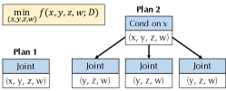
Figure 1. Two different execution plans for the same optimization problem. Each plan corresponds to a different way to decompose the same search space $(x,y,z,w)$.

VolcanoML Execution Plan

Due to space limitation, we omit the formal definition of a VolcanoML execution plan. Intuitively, a VolcanoML execution plan is a tree of building blocks. The root node corresponds to a building block solving the problem $f$ with the entire search space, which can be further decomposed into multiple building blocks if necessary, as previously described. As an example, Figure 1 illustrates two possible execution plans for $f(x,y,z,w;D)$. Plan 1 contains only a single root building block as a joint block, whereas Plan 2 first introduces a conditioning block on $x$, and then creates one lower level of building blocks for each possible value of $x$ (in Figure 1, we assume that $|\mathbb{D}_{x}|=3$).

VolcanoML Execution Model

To execute a VolcanoML execution plan, we follow a Volcano-style execution that is similar to a relational database (Graefe, 1994) — the system invokes the do_next! of the root node, which then invokes the do_next! of one of its child nodes, propagating until the leaf node. At any time, one can invoke the get_current_best of the root node, which returns the current best solution for the entire search space.

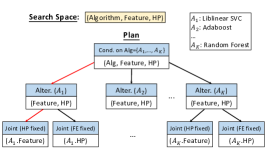
Figure 2. VolcanoML’s execution plan for the same search space as explored by auto-sklearn. Here ‘Alg’ and ‘HP’ correspond to Algorithm and hyper-parameters respectively.

VolcanoML Plan for auto-sklearn

Figure 2 presents a VolcanoML execution plan for the same search space explored by auto-sklearn, which consists of the joint search of algorithms, features, and hyper-parameters. Instead of conducting the search process in a single joint block, as was done by auto-sklearn, VolcanoML first decomposes the search space via a conditioning block on algorithms — this introduces a MAB problem in which each arm corresponds to one particular algorithm. It then further decomposes each of the conditioned subspaces via an alternating block between feature engineering and hyper-parameter tuning. The whole subspace of feature engineering (resp. that of hyper-parameter tuning) is optimized by a joint block.

Concretely, Figure 2 shows a search space for AutoML with $K$ choices of ML algorithms. During each iteration, starting from the root node, VolcanoML selects the child node to optimize until it reaches a leaf node, and then optimizes over the subspace in the leaf node. As shown by the red lines in Figure 2, in this iteration, VolcanoML only tunes the feature engineering pipeline of algorithm $A_{1}$ while fixing its algorithm hyper-parameters.

Alternative Execution Plans

Note that the execution plan in Figure 2 is not the only possible one. Our flexible and scalable framework in VolcanoML allows us to explore different execution plans before reaching the proposed one. We enumerate five possible plans in a coarse-grained level, and the results show that the proposed plan performs best. The reason why we choose this plan is due to the fundamental property of the AutoML search space — we observe that, the optimal choices of features are different across algorithms, which implies that we can first decompose the search space along ML algorithms. The improvements introduced by feature engineering and hyper-parameter tuning are largely complementary, and thus we can optimize them alternately. For feature engineering (resp. hyper-parameter tuning), the subspace is small enough to be handled by a single joint block efficiently.

VolcanoML Plan for Enriched Search Space

We can easily extend VolcanoML and enable functionalities that are not supported by most AutoML systems. For example, Figure 3 illustrates an execution plan for a search space with an additional stage — embedding selection. Given an input, e.g., image or text, we first choose embeddings based on a collection of TensorFlow Hub pre-trained models, and then conduct algorithm selection, feature engineering, and hyper-parameter tuning. We use an execution plan as illustrated in Figure 3, having the embedding selection step jointly optimized together with the feature engineering.

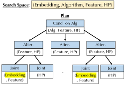
Figure 3. VolcanoML’s execution plan for a larger search space enriched by an additional embedding selection stage.

Discussion: Automatic Plan Generation. In principle, the design of VolcanoML opens up the opportunity for “automatic plan generation” — given a collection of benchmark datasets, one could automatically search for the best decomposition strategy of the search space and come up with a physical plan automatically. While the full treatment of this problem is beyond the scope of this paper, we illustrate the possibility with a very simple strategy. We automatically enumerate all possible execution plans in a coarse-grained level, and find that our manually specified execution plan in Figure 2 outperforms the alternatives. There is still an open question that whether we can support finer-grained partition of the search space (e.g., different plans for different subspace of features), and moreover, whether we can conduct efficient automatic plan optimization without enumerating all possible plans. These are exciting future directions and we expect the endeavor to be non-trivial. We hope that this paper sets the ground for this line of research in the future (e.g., rule-based heuristics or reinforcement learning).

Further Optimization with Meta-learning. VolcanoML supports meta-learning based techniques — given previous runs of the system over similar workloads, to transfer the knowledge and better help the workload at hand — to accelerate the optimization process of building blocks. Appendix contains the details.

5. Experimental Evaluation

We compare VolcanoML with state-of-the-art AutoML systems. In our evaluation, we focus on three perspectives: (1) the performance of VolcanoML given the same search space explored by existing systems, (2) the scalability of VolcanoML given larger search spaces, and (3) the extensibity of VolcanoML to integrate new components into the search space of AutoML pipelines.

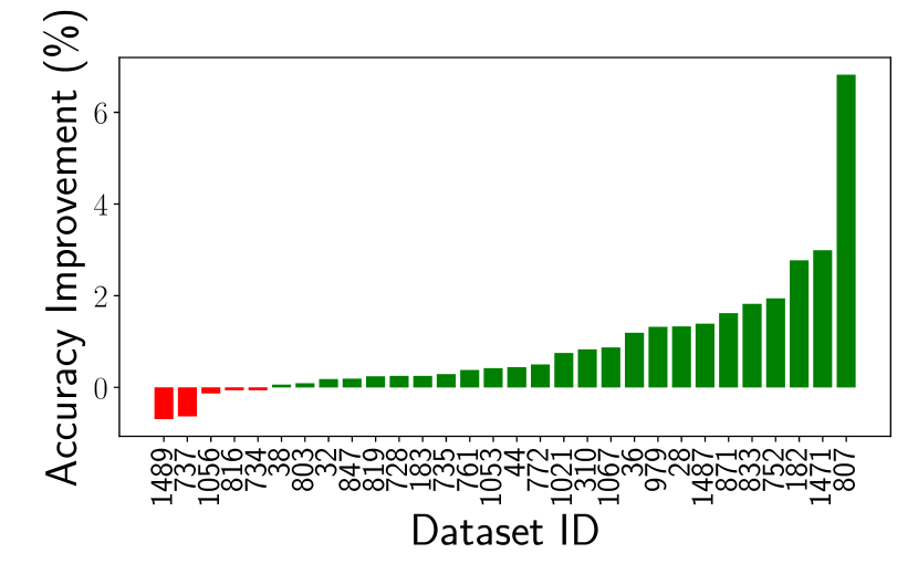
(a) VolcanoML vs. AUSK on CLS

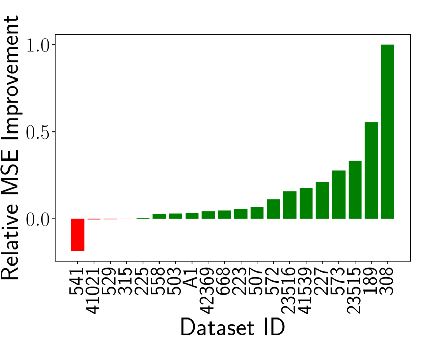
(b) VolcanoML vs. AUSK on REG

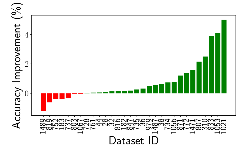
(c) VolcanoML vs. TPOT on CLS

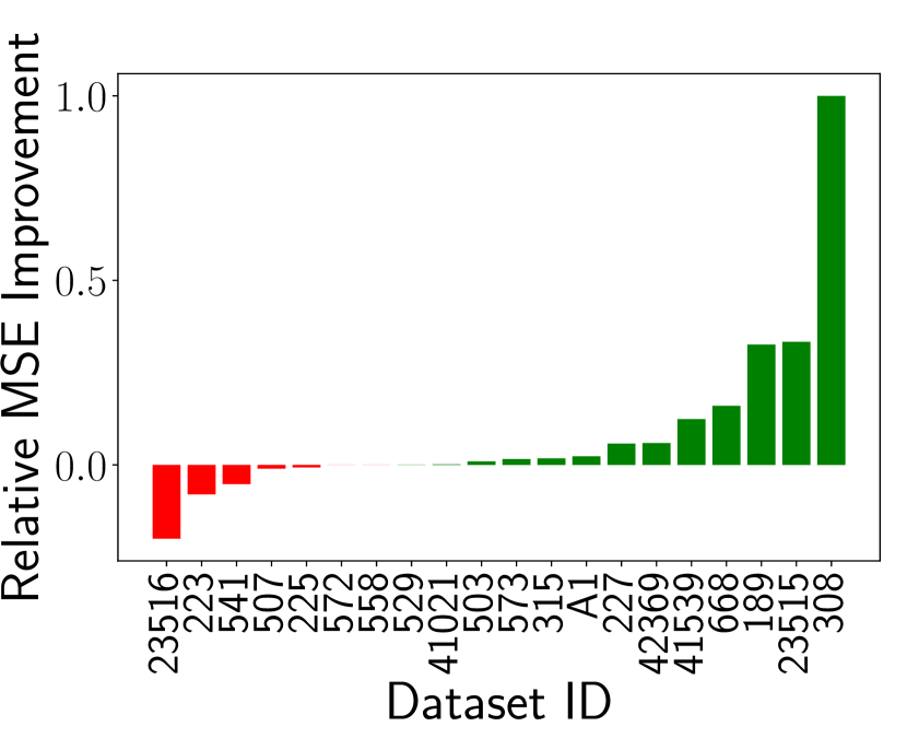
(d) VolcanoML vs. TPOT on REG

Figure 4. End-to-End results on 30 OpenML classification (CLS) datasets and 20 OpenML regression (REG) datasets.

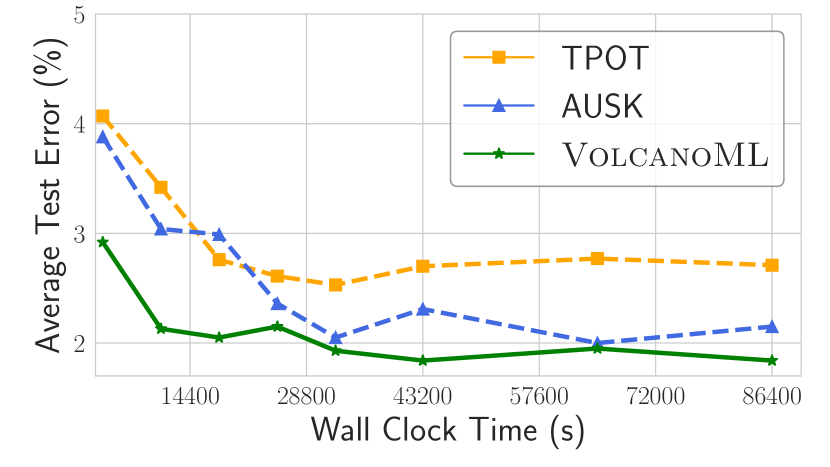
(a) Mnist_784

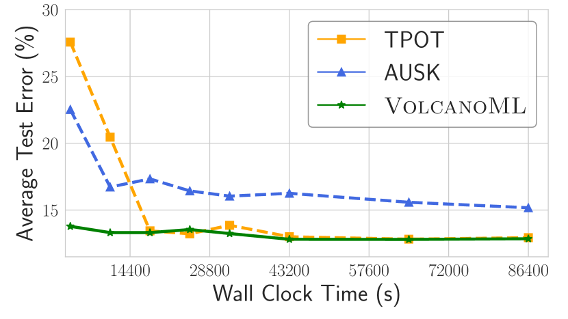
(b) Kropt

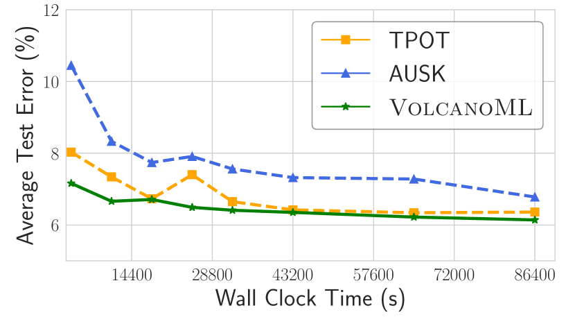
(c) Electricity

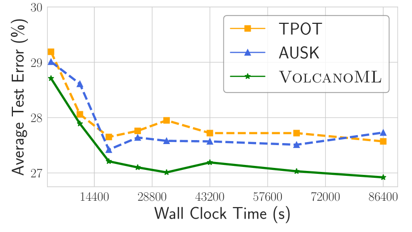
(d) Higgs

Figure 5. Average test errors on four large datasets with different time budgets.

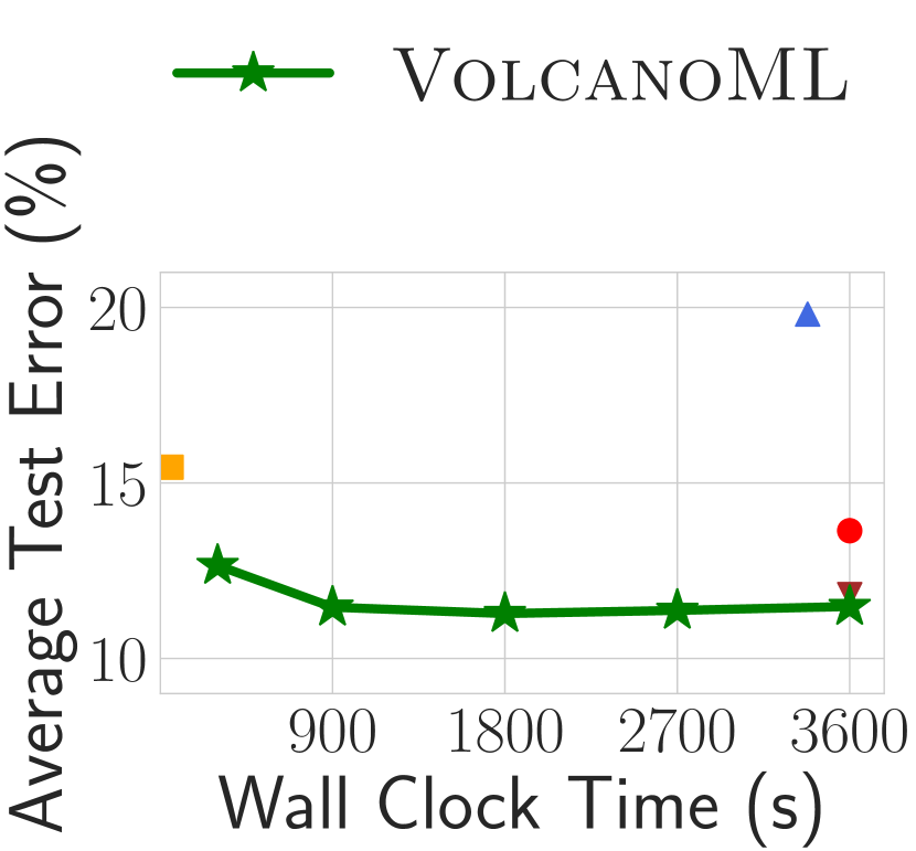
(a) Influence Network

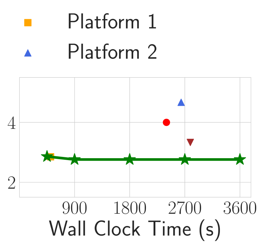
(b) Virus Prediction

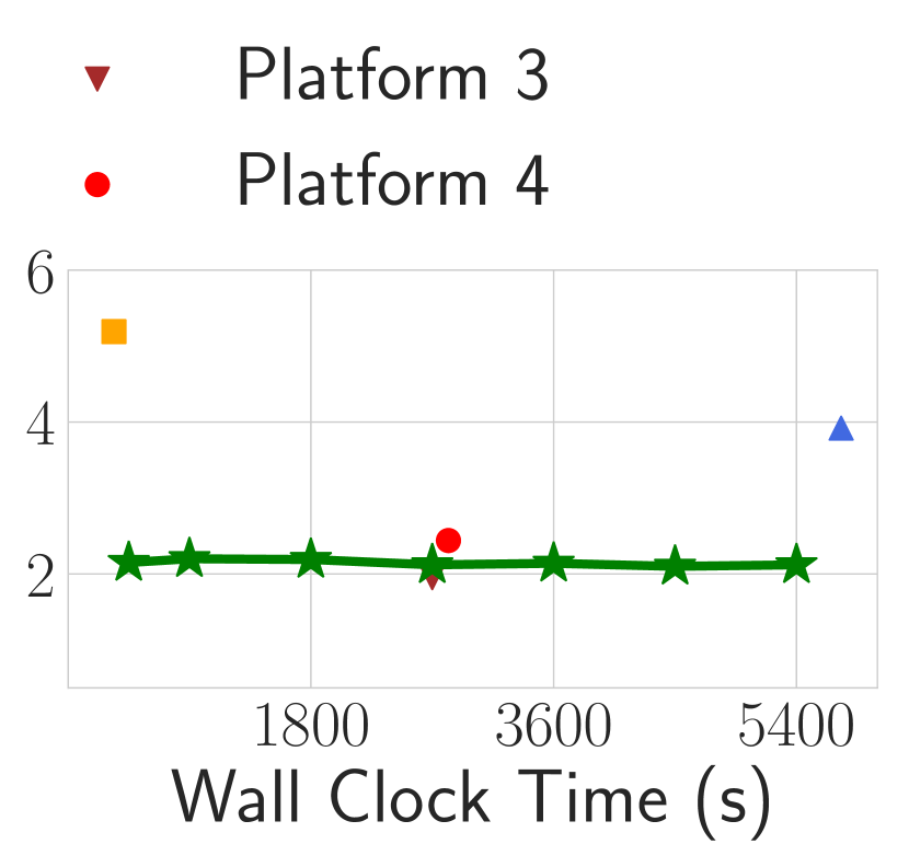
(c) Employee Access

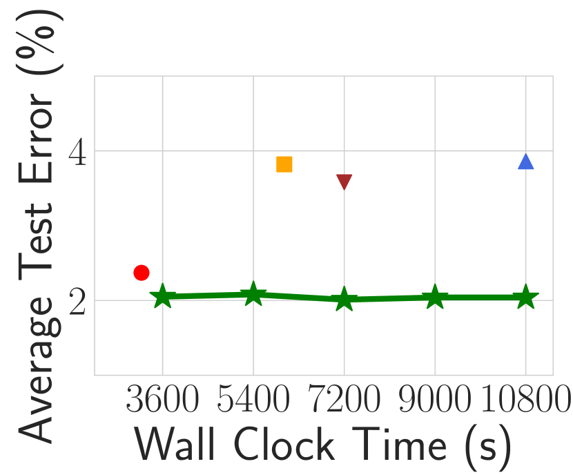
(d) Customer Satisfaction

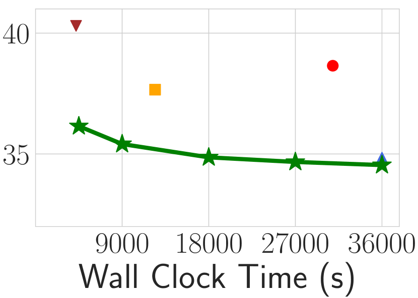
(e) Business Value

(f) Flavours

Figure 6. Test errors on 6 Kaggle competitions compared with four commercial platforms.

5.1. Experimental Setup

AutoML Systems.   We evaluate VolcanoML as well as two open source AutoML systems: auto-sklearn (Feurer et al., 2015) and TPOT (Olson and Moore, 2019). In addition, we also compare VolcanoML with four commercial AutoML platforms from Google, Amazon AWS, Microsoft Azure, and Oracle. Both VolcanoML and auto-sklearn support meta-learning, while TPOT does not. For fair comparison with TPOT, we also use $\textsc{VolcanoML}^{-}$ and AUSK^- to denote the versions of VolcanoML and auto-sklearn when meta-learning is disabled. Our implementation of VolcanoML is available at https://github.com/VolcanoML.

Datasets.   To compare VolcanoML with academic baselines, we use 60 real-world ML datasets from the OpenML repository (Vanschoren et al., 2014), including 40 for classification (CLS) tasks and 20 for regression (REG) tasks. 10 of the 40 classification datasets are relatively large, each with 20k to 110k data samples; the other 30 are of medium size, each with 1k to 12k samples. In addition, we also use datasets from six Kaggle competitions to compare VolcanoML with four commercial platforms.

AutoML Tasks.   We define three kinds of real-world AutoML tasks, including (1) a general classification task on 30 medium datasets, (2) a general regression task on 20 medium datasets, and (3) a large-scale classification task on 10 large datasets.

To test the scalability of the participating systems, we design three search spaces that include 20, 29, and 100 hyper-parameters, where the smaller search space is a subset of the larger one. We run VolcanoML and the baseline AutoML systems against each of the three search spaces. The time budget is 900 seconds for the smallest search space and 1,800 seconds for the other two, when performing the general classification task (1); the time budget is increased to 5,400 and 86,400 seconds respectively, when performing the general regression task (2) and the large-scale classification task (3).

Utility Metrics.   Following (Feurer et al., 2015), we adopt the metric balanced accuracy for all classification tasks — compared with standard (classification) accuracy, it assigns equal weights to classes and takes the average of class-wise accuracy. For regression tasks, we use the mean squared error (MSE) as the metric.

In our evaluation, we repeat each experiment 10 times and report the average utility metric. In each experiment, we use four fifths of the data samples in each dataset to search for the best ML pipeline and report the utility metric on the remaining fifth.

Search Space - Task	TPOT	AUSK-	AUSK	$\textsc{VolcanoML}^{-}$	VolcanoML
Small - CLS	3.09	3.07	3.01	2.94	2.89
Medium - CLS	3.2	3.32	3.27	2.78	2.43
Large - CLS	3.29	3.77	3.57	2.72	1.65
Small - REG	2.98	3.02	3.0	3.02	2.98
Medium - REG	2.95	3.3	3.12	2.75	2.88
Large - REG	3.1	3.85	3.82	2.15	2.08

Table 1. Average ranks on 30 classification (CLS) datasets and 20 regression (REG) datasets with three different search spaces. (The lower is the better)

Methodology for Comparing AutoML Systems.   To compare the overall test result of each AutoML system on a wide range of datasets, we use the average rank as the metric following (Bardenet et al., 2013). For each dataset, we rank all participant systems based on the result of the best ML pipeline they have found so far; we then take the average of their ranks across different datasets.

More Details.   We include the details of search space and programming API, experiment settings and additional experiments, and reproductions in the Appendix.

5.2. End-to-End Comparison

We first evaluate the participant AutoML systems given the search space explored by auto-sklearn. Figure 4 presents the results of VolcanoML compared to auto-sklearn (AUSK) and TPOT on the 30 classification tasks and the 20 regression tasks, respectively. For classification tasks, we plot the classification accuracy improvement (%); for regression tasks, we plot the relative MSE improvement $\Delta$, which is defined as $\Delta(m_{1},m_{2})=\frac{s(m_{2})-s(m_{1})}{\operatorname{max}(s(m_{2}),s(m_{1}))}$, where $s(\cdot)$ is MSE on the test set. Overall, VolcanoML outperforms auto-sklearn and TPOT on 25 and 23 of the 30 classification tasks, and on 17 and 15 of the 20 regression tasks, respectively.

We also conduct experiments to evaluate VolcanoML with different time budgets. Figure 5 presents the results on four large classification datasets. We observe that VolcanoML exhibits consistent performance over different time budgets. Notably, on Higgs, VolcanoML achieves $27.2$% test error within 4 hours, which is better than the performance of the other two systems given 24 hours.

We further study the scalability of the participant systems on the three aforementioned search spaces. Table 1 summarizes the results in terms of the average ranks. We have two observations: First, without meta-learning, VolcanoML achieves the best average rank for both the classification and regression tasks — on the small search space (with 20 hyper-parameters), VolcanoML performs slightly better than auto-sklearn and TPOT, and it performs significantly better on the medium (with 29 hyper-parameters) and large (with 100 hyper-parameters) search spaces. Second, with meta-learning, the average rank of VolcanoML is dramatically improved compared with auto-sklearn. Overall, VolcanoML with meta-learning achieves the best result over large search space. Furthermore, we also design additional experiments to evaluate the consistency of system performance given different (larger) time budgets and search spaces, and more details can be found in Appendix.

5.3. Search Space Enrichment

We now focus on evaluating the extensibility of VolcanoML via two experiments with enriched search spaces.

Adding Data_Balancing Operator. In the first experiment, we implement “smote_balancer” – a new feature engineering operator, and incorporate it into the aforementioned balancing stage of feature engineering (FE) (Section 3.1). Note that auto-sklearn cannot support this fine-grained enrichment of the search space. Table 2 presents the results of auto-sklearn, VolcanoML without enrichment, and VolcanoML with enrichment, on five imbalanced datasets. We observe that enriching the search space brings further improvement, e.g., VolcanoML with enrichment outperforms auto-sklearn by 3.57% (balanced accuracy) on the dataset pc2.

Supporting Embedding Selection. In the second experiment, we add a new stage “embedding selection” into the FE pipeline, with two candidate embedding-extraction operators (i.e., two pre-trained models). This allows VolcanoML to deal with images, which are not easily supported by both auto-sklearn and TPOT. We implement two pre-trained models to generate embeddings for images, and we evaluate VolcanoML with the enriched search space on the Kaggle dataset dogs-vs-cats. We observe that VolcanoML achieves 96.5% test accuracy, which is significantly better than 69.7% obtained by auto-sklearn without considering embeddings.

Dataset	AUSK	$\textsc{VolcanoML}^{-}$	VolcanoML
sick	97.29	97.31	97.34
pc2	86.70	86.91	90.27
abalone	66.86	65.97	67.32
page-blocks(2)	94.70	95.29	96.69
hypothyroid(2)	99.62	99.64	99.64

Table 2. Test accuracy (%) of VolcanoML with and without the enrichment of “smote_balancer” operator.

5.4. Comparison with 4 Industrial Platforms

In addition, we run additional experiments on six Kaggle datasets to compare VolcanoML with four commercial AutoML platforms: 1) Google Cloud AutoML, 2) Microsoft Azure Automated ML, 3) Oracle data science, and 4) Amazon AWS Sagemaker AutoPilot. Here, we anonymously refer to these platforms as Platform 1-4. Figure 6 show the results, and the Appendix contains the experiment details. We observe that, given the same time budget (i.e., fix the x-axis to some time budget), VolcanoML is at least comparable with, often outperforms, the considered commercial platforms.

6. Conclusion

In this paper, we have presented VolcanoML, a scalable and extensible framework that allows users to design decomposition strategies for large AutoML search spaces in an expressive and flexible manner. VolcanoML introduces novel building blocks akin to relational operators in database systems that enable expressing search space decomposition strategies in a structured fashion – similar to relational execution plans. Moreover, VolcanoML introduces a Volcano-style execution model, inspired by its classic counterpart that has been widely used for relational query evaluation, to execute the decomposition strategies it yields. Experimental evaluation demonstrates that VolcanoML can generate more efficient decomposition strategies that also lead to performance-wise better ML pipelines, compared to state-of-the-art AutoML systems.

References

- (1)
- Bardenet et al. (2013) Rémi Bardenet, Mátyás Brendel, Balázs Kégl, and Michele Sebag. 2013. Collaborative hyperparameter tuning. In International Conference on Machine Learning. 199–207.
- Barnes (2015) Jeff Barnes. 2015. Azure machine learning. Microsoft Azure Essentials. 1st ed, Microsoft (2015).
- Bergstra and Bengio (2012) James Bergstra and Yoshua Bengio. 2012. Random search for hyper-parameter optimization. Journal of Machine Learning Research 13, Feb (2012), 281–305.
- Bergstra et al. (2011) James S Bergstra, Rémi Bardenet, Yoshua Bengio, and Balázs Kégl. 2011. Algorithms for hyper-parameter optimization. In Advances in neural information processing systems. 2546–2554.
- Boehm et al. (2019) Matthias Boehm, Iulian Antonov, Mark Dokter, Robert Ginthör, Kevin Innerebner, Florijan Klezin, Stefanie Lindstaedt, Arnab Phani, and Benjamin Rath. 2019. SystemDS: A declarative machine learning system for the end-to-end data science lifecycle. arXiv:1909.02976
- Breck et al. (2019) Eric Breck et al. 2019. Data Validation for Machine Learning. In SysML.
- CarøE and Schultz (1999) Claus C CarøE and Rüdiger Schultz. 1999. Dual decomposition in stochastic integer programming. Operations Research Letters 24, 1-2 (1999), 37–45.
- Chen et al. (2018) Boyuan Chen, Harvey Wu, Warren Mo, and Ishanu Chattopadhyay. 2018. Autostacker: A compositional evolutionary learning system. In GECCO 2018 - Proceedings of the 2018 Genetic and Evolutionary Computation Conference. https://doi.org/10.1145/3205455.3205586 arXiv:1803.00684
- de Sá et al. (2017) Alex G.C. de Sá, Walter José G.S. Pinto, Luiz Otavio V.B. Oliveira, and Gisele L. Pappa. 2017. RECIPE: A grammar-based framework for automatically evolving classification pipelines. In Lecture Notes in Computer Science (including subseries Lecture Notes in Artificial Intelligence and Lecture Notes in Bioinformatics). https://doi.org/10.1007/978-3-319-55696-3_16
- Dechter (1998) Rina Dechter. 1998. Bucket elimination: A unifying framework for probabilistic inference. In Learning in graphical models. Springer, 75–104.
- Drori et al. (2018) Iddo Drori, Yamuna Krishnamurthy, Remi Rampin, Raoni De, Paula Lourenco, Jorge Piazentin Ono, Kyunghyun Cho, Claudio Silva, and Juliana Freire. 2018. AlphaD3M: Machine Learning Pipeline Synthesis. AutoML Workshop at ICML (2018).
- Efimova et al. (2017) Valeria Efimova, Andrey Filchenkov, and Viacheslav Shalamov. 2017. Fast Automated Selection of Learning Algorithm And its Hyperparameters by Reinforcement Learning. In International Conference on Machine Learning AutoML Workshop.
- Eggensperger et al. (2013) Katharina Eggensperger, Matthias Feurer, Frank Hutter, James Bergstra, Jasper Snoek, Holger Hoos, and Kevin Leyton-Brown. 2013. Towards an empirical foundation for assessing bayesian optimization of hyperparameters. In NIPS workshop on Bayesian Optimization in Theory and Practice, Vol. 10. 3.
- Falkner et al. (2018) Stefan Falkner, Aaron Klein, and Frank Hutter. 2018. BOHB: Robust and efficient hyperparameter optimization at scale. arXiv preprint arXiv:1807.01774 (2018).
- Feurer et al. (2015) Matthias Feurer, Aaron Klein, Katharina Eggensperger, Jost Springenberg, Manuel Blum, and Frank Hutter. 2015. Efficient and robust automated machine learning. In Advances in neural information processing systems. 2962–2970.
- Feurer et al. (2018) Matthias Feurer, Benjamin Letham, and Eytan Bakshy. 2018. Scalable meta-learning for bayesian optimization using ranking-weighted gaussian process ensembles. In AutoML Workshop at ICML.
- Garcia-Molina et al. (2008) Hector Garcia-Molina, Jeffrey D. Ullman, and Jennifer Widom. 2008. Database Systems: The Complete Book (2 ed.). Prentice Hall Press, USA.
- Ghoting et al. (2011) Amol Ghoting, Rajasekar Krishnamurthy, Edwin Pednault, Berthold Reinwald, Vikas Sindhwani, Shirish Tatikonda, Yuanyuan Tian, and Shivakumar Vaithyanathan. 2011. SystemML: Declarative machine learning on MapReduce. In Proceedings - International Conference on Data Engineering. https://doi.org/10.1109/ICDE.2011.5767930
- Golovin et al. (2017) Daniel Golovin, Benjamin Solnik, Subhodeep Moitra, Greg Kochanski, John Karro, and D Sculley. 2017. Google vizier: A service for black-box optimization. In Proceedings of the 23rd ACM SIGKDD International Conference on Knowledge Discovery and Data Mining. ACM, 1487–1495.
- Google (2020) Google. 2020. Google Prediction API,. https://developers.google.com/prediction.
- Graefe (1994) Goetz Graefe. 1994. Volcano—An Extensible and Parallel Query Evaluation System. IEEE Transactions on Knowledge and Data Engineering (1994). https://doi.org/10.1109/69.273032
- He et al. (2020) Xin He, Kaiyong Zhao, and Xiaowen Chu. 2020. AutoML: A Survey of the State-of-the-Art. arXiv:1908.00709 [cs.LG]
- Hu et al. (2019) Yi-Qi Hu, Yang Yu, Wei-Wei Tu, Qiang Yang, Yuqiang Chen, and Wenyuan Dai. 2019. Multi-Fidelity Automatic Hyper-Parameter Tuning via Transfer Series Expansion. AAAI (2019).
- Hutter et al. (2014) Frank Hutter, Hoiger Hoos, and Kevin Leyton-Brown. 2014. An efficient approach for assessing hyperparameter importance. In 31st International Conference on Machine Learning, ICML 2014.
- Hutter et al. (2011) Frank Hutter, Holger H Hoos, and Kevin Leyton-Brown. 2011. Sequential model-based optimization for general algorithm configuration. In International Conference on Learning and Intelligent Optimization. Springer, 507–523.
- Hutter et al. (2018) Frank Hutter, Lars Kotthoff, and Joaquin Vanschoren (Eds.). 2018. Automated Machine Learning: Methods, Systems, Challenges. Springer. In press, available at http://automl.org/book.
- Hutter et al. (2015) Frank Hutter, Jörg Lücke, and Lars Schmidt-Thieme. 2015. Beyond Manual Tuning of Hyperparameters. KI - Kunstliche Intelligenz (2015). https://doi.org/10.1007/s13218-015-0381-0
- IBM (2020) IBM. 2020. IBMWatson Studio AutoAI. https://www.ibm.com/cloud/watson-studio/autoai.
- Jamieson and Talwalkar (2016) Kevin Jamieson and Ameet Talwalkar. 2016. Non-stochastic best arm identification and hyperparameter optimization. In Artificial Intelligence and Statistics. 240–248.
- Jones et al. (1998) Donald R Jones, Matthias Schonlau, and William J Welch. 1998. Efficient global optimization of expensive black-box functions. Journal of Global optimization 13, 4 (1998), 455–492.
- Kandasamy et al. (2017) Kirthevasan Kandasamy, Gautam Dasarathy, Jeff Schneider, and Barnabas Poczos. 2017. Multi-fidelity bayesian optimisation with continuous approximations. arXiv preprint arXiv:1703.06240 (2017).
- Kanter and Veeramachaneni (2015) James Max Kanter and Kalyan Veeramachaneni. 2015. Deep feature synthesis: Towards automating data science endeavors. In 2015 IEEE International Conference on Data Science and Advanced Analytics, DSAA 2015, Paris, France, October 19-21, 2015. IEEE, 1–10.
- Katz et al. (2017) Gilad Katz, Eui Chul Richard Shin, and Dawn Song. 2017. ExploreKit: Automatic feature generation and selection. In Proc. - IEEE Int. Conf. Data Mining, ICDM. https://doi.org/10.1109/ICDM.2016.176
- Kaul et al. (2017) Ambika Kaul, Saket Maheshwary, and Vikram Pudi. 2017. Autolearn - automated feature generation and selection. In Proc. - IEEE Int. Conf. Data Mining, ICDM, Vol. 2017-Novem. https://doi.org/10.1109/ICDM.2017.31
- Khurana et al. (2018) Udayan Khurana, Horst Samulowitz, and Deepak Turaga. 2018. Feature engineering for predictive modeling using reinforcement learning. In 32nd AAAI Conf. Artif. Intell. AAAI 2018.
- Khurana et al. (2016) Udayan Khurana, Deepak Turaga, Horst Samulowitz, and Srinivasan Parthasrathy. 2016. Cognito: Automated Feature Engineering for Supervised Learning. In IEEE Int. Conf. Data Min. Work. ICDMW, Vol. 0. https://doi.org/10.1109/ICDMW.2016.0190
- Klein et al. (2017) Aaron Klein, Stefan Falkner, Simon Bartels, Philipp Hennig, and Frank Hutter. 2017. Fast Bayesian Optimization of Machine Learning Hyperparameters on Large Datasets. In Proceedings of the 20th International Conference on Artificial Intelligence and Statistics. 528–536.
- Komer et al. (2014) Brent Komer, James Bergstra, and Chris Eliasmith. 2014. Hyperopt-sklearn: automatic hyperparameter configuration for scikit-learn. In ICML workshop on AutoML, Vol. 9. Citeseer.
- Kraska (2018) Tim Kraska. 2018. Northstar: An Interactive Data Science System. PVLDB (2018).
- Krishnan et al. (2016) Sanjay Krishnan et al. 2016. ActiveClean: Interactive Data Cleaning for Statistical Modeling. PVLDB (2016).
- LeDell and Poirier (2020) Erin LeDell and S Poirier. 2020. H2o automl: Scalable automatic machine learning. In Proceedings of the AutoML Workshop at ICML, Vol. 2020.
- Levine et al. (2017) Nir Levine, Koby Crammer, and Shie Mannor. 2017. Rotting bandits. In Advances in NIPS. 3074–3083.
- Li et al. (2018b) Lisha Li, Kevin Jamieson, Giulia DeSalvo, Afshin Rostamizadeh, and Ameet Talwalkar. 2018b. Hyperband: A novel bandit-based approach to hyperparameter optimization. Proceedings of the International Conference on Learning Representations (2018), 1–48.
- Li et al. (2018a) Tian Li et al. 2018a. Ease.ml: Towards Multi-tenant Resource Sharing for Machine Learning Workloads. In PVLDB.
- Li et al. (2020a) Yang Li, Jiawei Jiang, Jinyang Gao, Yingxia Shao, Ce Zhang, and Bin Cui. 2020a. Efficient Automatic CASH via Rising Bandits.. In AAAI. 4763–4771.
- Li et al. (2020b) Yang Li, Jiawei Jiang, Jinyang Gao, Yingxia Shao, Ce Zhang, and Bin Cui. 2020b. Efficient Automatic CASH via Rising Bandits. In The Thirty-Fourth AAAI Conference on Artificial Intelligence, AAAI 2020, The Thirty-Second Innovative Applications of Artificial Intelligence Conference, IAAI 2020, The Tenth AAAI Symposium on Educational Advances in Artificial Intelligence, EAAI 2020, New York, NY, USA, February 7-12, 2020. AAAI Press, 4763–4771. https://aaai.org/ojs/index.php/AAAI/article/view/5910
- Li et al. (2020c) Yang Li, Yu Shen, Jiawei Jiang, Jinyang Gao, Ce Zhang, and Bin Cui. 2020c. MFES-HB: Efficient Hyperband with Multi-Fidelity Quality Measurements. arXiv:2012.03011 [cs.LG]
- Liaw et al. (2018) Richard Liaw, Eric Liang, Robert Nishihara, Philipp Moritz, Joseph E Gonzalez, and Ion Stoica. 2018. Tune: A Research Platform for Distributed Model Selection and Training. arXiv preprint arXiv:1807.05118 (2018).
- Liberty et al. (2020) Edo Liberty, Zohar Karnin, Bing Xiang, Laurence Rouesnel, Baris Coskun, Ramesh Nallapati, Julio Delgado, Amir Sadoughi, Yury Astashonok, Piali Das, et al. 2020. Elastic Machine Learning Algorithms in Amazon SageMaker. In Proceedings of the 2020 ACM SIGMOD International Conference on Management of Data. 731–737.
- Liu et al. (2020) Sijia Liu, Parikshit Ram, Djallel Bouneffouf, Gregory Bramble, Andrew R Conn, Horst Samulowitz, and Alexander G Gray. 2020. An ADMM Based Framework for AutoML Pipeline Configuration. (2020), 4892–4899.
- Modi et al. (2017) Akshay Naresh Modi et al. 2017. TFX: A TensorFlow-Based Production-Scale Machine Learning Platform. In KDD 2017.
- Mohr et al. (2018) Felix Mohr, Marcel Wever, and Eyke Hüllermeier. 2018. ML-Plan: Automated machine learning via hierarchical planning. Machine Learning (2018). https://doi.org/10.1007/s10994-018-5735-z
- Moritz et al. (2007) Philipp Moritz, Robert Nishihara, Stephanie Wang, Alexey Tumanov, Richard Liaw, Eric Liang, Melih Elibol, Zongheng Yang, William Paul, Michael I. Jordan, and Ion Stoica. 2007. Ray: A distributed framework for emerging AI applications. In Proceedings of the 13th USENIX Symposium on Operating Systems Design and Implementation, OSDI 2018. arXiv:1712.05889
- Nakandala et al. (2019) Supun Nakandala et al. 2019. Incremental and Approximate Inference for Faster Occlusion-Based Deep CNN Explanations. In SIGMOD.
- Nakandala et al. (2020) Supun Nakandala et al. 2020. Cerebro: A Data System for Optimized Deep Learning Model Selection. PVLDB (2020).
- Nargesian et al. (2017) Fatemeh Nargesian, Horst Samulowitz, Udayan Khurana, Elias B. Khalil, and Deepak Turaga. 2017. Learning feature engineering for classification. In IJCAI Int. Jt. Conf. Artif. Intell., Vol. 0. https://doi.org/10.24963/ijcai.2017/352
- Olson and Moore (2019) Randal S Olson and Jason H Moore. 2019. TPOT: A tree-based pipeline optimization tool for automating machine learning. In Automated Machine Learning. Springer, 151–160.
- Poloczek et al. (2017) Matthias Poloczek, Jialei Wang, and Peter Frazier. 2017. Multi-information source optimization. In Advances in Neural Information Processing Systems. 4288–4298.
- Ratner et al. (2017) Alexander Ratner et al. 2017. Snorkel: Rapid Training Data Creation with Weak Supervision. PVLDB (2017).
- Rekatsinas et al. (2017) Theodoros Rekatsinas et al. 2017. HoloClean: Holistic Data Repairs with Probabilistic Inference. PVLDB (2017).
- Research (2020) Microsoft Research. 2020. Microsoft NNI. https://github.com/Microsoft/nni.
- Schawinski et al. (2017) Kevin Schawinski et al. 2017. Generative Adversarial Networks recover features in astrophysical images of galaxies beyond the deconvolution limit. MNRAS Letters (2017).
- Sen et al. (2018) Rajat Sen, Kirthevasan Kandasamy, and Sanjay Shakkottai. 2018. Noisy Blackbox Optimization with Multi-Fidelity Queries: A Tree Search Approach. arXiv: Machine Learning (2018).
- Shahriari et al. (2016) Bobak Shahriari, Kevin Swersky, Ziyu Wang, Ryan P. Adams, and Nando De Freitas. 2016. Taking the human out of the loop: A review of Bayesian optimization. https://doi.org/10.1109/JPROC.2015.2494218
- Snoek et al. (2012) Jasper Snoek, Hugo Larochelle, and Ryan P Adams. 2012. Practical bayesian optimization of machine learning algorithms. In Advances in neural information processing systems. 2951–2959.
- Swersky et al. (2013) Kevin Swersky, Jasper Snoek, and Ryan P Adams. 2013. Multi-task bayesian optimization. In Advances in neural information processing systems. 2004–2012.
- Takeno et al. (2020) Shion Takeno, Hitoshi Fukuoka, Yuhki Tsukada, Toshiyuki Koyama, Motoki Shiga, Ichiro Takeuchi, and Masayuki Karasuyama. 2020. Multi-fidelity Bayesian Optimization with Max-value Entropy Search and its parallelization. arXiv:1901.08275 [stat.ML]
- Thornton et al. (2013) C. Thornton, F. Hutter, H. H. Hoos, and K. Leyton-Brown. 2013. Auto-WEKA: Combined Selection and Hyperparameter Optimization of Classification Algorithms. In Proc. of KDD-2013. 847–855.
- Van Rijn and Hutter (2018) Jan N. Van Rijn and Frank Hutter. 2018. Hyperparameter importance across datasets. In Proceedings of the ACM SIGKDD International Conference on Knowledge Discovery and Data Mining. https://doi.org/10.1145/3219819.3220058 arXiv:1710.04725
- Vanschoren (2018) Joaquin Vanschoren. 2018. Meta-Learning: A Survey. CoRR abs/1810.03548 (2018). arXiv:1810.03548 http://arxiv.org/abs/1810.03548
- Vanschoren et al. (2014) Joaquin Vanschoren, Jan N. van Rijn, Bernd Bischl, and Luis Torgo. 2014. OpenML: Networked Science in Machine Learning. SIGKDD Explor. Newsl. 15, 2 (June 2014), 49–60. https://doi.org/10.1145/2641190.2641198
- Vartak et al. (2016) Manasi Vartak et al. 2016. ModelDB: A System for Machine Learning Model Management. In HILDA.
- Wang et al. (2013) Ziyu Wang, Masrour Zoghi, Frank Hutter, David Matheson, and Nando De Freitas. 2013. Bayesian optimization in high dimensions via random embeddings. In Twenty-Third International Joint Conference on Artificial Intelligence.
- Wistuba et al. (2016) Martin Wistuba, Nicolas Schilling, and Lars Schmidt-Thieme. 2016. Two-stage transfer surrogate model for automatic hyperparameter optimization. In Joint European conference on machine learning and knowledge discovery in databases. Springer, 199–214.
- Wu et al. (2019a) Jian Wu, Saul Toscano-Palmerin, Peter I. Frazier, and Andrew Gordon Wilson. 2019a. Practical multi-fidelity Bayesian optimization for hyperparameter tuning. arXiv:1903.04703
- Wu et al. (2019b) Jian Wu, Saul Toscanopalmerin, Peter I Frazier, and Andrew Gordon Wilson. 2019b. Practical multi-fidelity Bayesian optimization for hyperparameter tuning. (2019), 284.
- Wu et al. (2020a) Renzhi Wu et al. 2020a. ZeroER: Entity Resolution Using Zero Labeled Examples. In SIGMOD.
- Wu et al. (2020b) Weiyuan Wu et al. 2020b. Complaint-Driven Training Data Debugging for Query 2.0. In SIGMOD.
- Yao et al. (2018) Quanming Yao, Mengshuo Wang, Hugo Jair Escalante, Isabelle Guyon, Yi-Qi Hu, Yu-Feng Li, Wei-Wei Tu, Qiang Yang, and Yang Yu. 2018. Taking Human out of Learning Applications: A Survey on Automated Machine Learning. CoRR (2018).
- Zaharia et al. (2018) M. Zaharia et al. 2018. Accelerating the Machine Learning Lifecycle with MLflow. IEEE Data Eng. Bull. (2018).
- Zhang et al. (2017) Ce Zhang et al. 2017. DeepDive: Declarative Knowledge Base Construction. Commun. ACM (2017).
- Zöller and Huber (2019) Marc-André Zöller and Marco F. Huber. 2019. Survey on Automated Machine Learning. CoRR abs/1904.12054 (2019).