Multiparameter persistent homology via generalized Morse theory

Abstract

We define a class of multiparameter persistence modules that arise from a one-parameter family of functions on a topological space and prove that these persistence modules are stable. We show that this construction can produce indecomposable persistence modules with arbitrarily large dimension. In the case of smooth functions on a compact manifold, we apply cobordism theory and Cerf theory to study the resulting persistence modules. We give examples in which we obtain a complete description of the persistence module as a direct sum of indecomposable summands and provide a corresponding visualization.

1 Introduction

Persistent homology is an important tool in topological data analysis, whose goal is to use ideas from topology to understand the ‘shape of data’ [12, 7].

An important example of persistent homology starts with a smooth, compact manifold $M$ and a Morse function $f:M\to\mathbb{R}$. Classical Morse theory concerns itself with the study of $M$ via the critical points of $f$ by analyzing the sublevel sets $F(a)=f^{-1}(\infty,a]$ and how their topology changes as $a$ varies. The subspaces $\{F(a)\}_{a\in\mathbb{R}}$ and their inclusion maps may be used to define a functor $F:\mathbf{R}\to\mathbf{Top}$, where $\mathbf{R}$ is the category given by the linear order on $\mathbb{R}$ and $\mathbf{Top}$ is the category of topological spaces and continuous maps. Composing with singular homology in some degree $j$ and coefficients in a field $k$ we obtain a functor $H_{j}F:\mathbf{R}\to\mathbf{Vect_{k}}$ with codomain the category of $k$-vector spaces and $k$-linear maps. Such a functor is called a persistence module.

Let $\beta_{j}$ denote the $j$-th Betti number of $M$ and let $M_{j}$ denote the number of critical points of index of $j$ of $f$. Let $M(t)=\sum_{j}M_{j}t^{j}$ and $\beta(t)=\sum_{j}\beta_{j}t^{j}$. Morse observed that $M(t)-\beta(t)=(1+t)D(t)$ for some polynomial $D(t)$ with non-negative coefficients [29]. That is, the excess of critical points of the Morse function come in pairs that differ in index by one. A strengthening of this observation is a central result in persistent homology. The persistence module $H_{j}F$ decomposes into a direct sum of indecomposable summands given by one-dimensional vector spaces supported on an interval. The end points of these intervals are exactly the critical values of the paired critical points in Morse’s theorem. This pairing of critical values, called the persistence diagram, is central to persistent homology.

While this setting has been very successful, in many applications the data are best described not by a single function $f:M\to\mathbb{R}$ but by a one-parameter family of functions $f_{t}:M\to\mathbb{R}$, where $t\in I=[0,1]$. For example, one may handle noise in the data with a procedure dependent on a parameter $t$. The resulting homological data may be encoded in a multiparameter persistence module. However, in general this module does not decompose into one-dimensional summands, and there is no complete invariant analogous to the persistence diagram [8].

We approach multiparameter persistent homology using two distinct generalizations of Morse theory. The first is a parametrized approach to Morse theory, known as Cerf theory. Cerf theory was initiated by J. Cerf in his celebrated proof of the Pseudo-Isotopy Theorem [9]. One outcome of his work was a useful stratification on the space of all smooth functions on a smooth compact manifold, stratified by singularity type. The existence of this stratification implies that generic, 1-parameter families of smooth functions are almost always Morse, except for finitely many parameter values at which the function may have cubic, or ‘birth-death’ type, singularities. Cerf developed a convenient framework for understanding how singularities merge, split, and pass one another in families. This understanding is paramount for our analysis.

The second variant is Morse theory adapted to the case of manifolds with boundary. This was developed around the same time as Cerf theory but by several authors independently [14, 2, 19]. Many statements in classical Morse theory can be adapted to manifolds with boundary, so long as the gradient or gradient-like flow used is tangent to the boundary. Critical points occurring on the interior behave as one expects, but on the boundary they come in two distinct flavors, either stable or unstable, depending on the local flow. Altogether, Morse theory for manifolds with boundary is a powerful extension of its classical analog. We have only touched the surface of using this subject in multiparameter persistence.

Our contributions

Given a topological space $X$ and a one-parameter family of (not necessarily continuous) functions $\tilde{f}:I\times X\to\mathbb{R}$, we define a fibered version of $\tilde{f}$ by letting $f:I\times X\to I\times\mathbb{R}$ be given by $f(t,x)=(t,\tilde{f}(t,x))$. The collection of subspaces

$$F(a,b,c)=f^{-1}([a,b]\times(-\infty,c])\subset I\times X\,,$$ (1)

for $0\leq a\leq b\leq 1$ and $c\in\mathbb{R}$, are our main objects of study. For $[a,b]\subset[a^{\prime},b^{\prime}]$ and $c\leq c^{\prime}$ there is an inclusion of $F(a,b,c)$ into $F(a^{\prime},b^{\prime},c^{\prime})$. These topological spaces and continuous maps describe a functor $F:\mathbf{Int_{I}\times R}\to\mathbf{Top}$, where $\mathbf{Int_{I}\times R}$ is the category given by the product of the partial order on the closed intervals in $I$ and the linear order on $\mathbb{R}$. Composing with singular homology in some degree $j$ with coefficients in a field $k$, we obtain a functor $H_{j}F:\mathbf{Int_{I}\times R}\to\mathbf{Vect_{k}}$. This functor is a multiparameter persistence module.

We prove that this functor is stable with respect to the interleaving distance for perturbations of the one-parameter family of smooth functions (Theorem 3.2).

We consider several examples of such one-parameter families of functions and give complete descriptions of their multiparameter persistence modules (Sections 4.1, 4.3, 4.4, and 6). In particular, we give decompositions of these modules into their indecomposable summands and provide corresponding visualizations (Figures 5, 7, and 10). We also show that indecomposable persistent modules arising from one-parameter families of functions may have arbitrarily large dimension (Section 4.2).

Now consider the case where $X$ is a smooth compact manifold and $\tilde{f}$ is smooth. Let $F_{0}(a,b,c)=f^{-1}([a,b]\times\{c\})$. We prove (Theorem 5.2) that for generic $a$, $b$, and $c$, $(F(a,b,c),F_{0}(a,b,c))$ forms a cobordism between the manifolds with boundary $(F(a,a,c),F_{0}(a,a,c))$ and $(F(b,b,c),F_{0}(b,b,c)$. Furthermore, it is naturally equipped with a Morse function

$$\pi_{[a,b]}:F(a,b,c)\to[a,b]\,,$$

given by projection onto the interval $[a,b]$. This Morse function has no critical points on $F(a,b,c)\setminus F_{0}(a,b,c)$ and the positive and negative critical points on $F_{0}(a,b,c)$ (Definition 5.1) correspond to boundary stable and boundary unstable critical points, respectively.

We remark that if we restrict our collection of subspaces in (1) to those with $a=0$ then we obtain a multiparameter persistence module indexed by $I\times\mathbb{R}\subset\mathbb{R}^{2}$, with the usual product partial order. However, this two-parameter persistence module is a weaker invariant than our three-parameter persistence module. For example, if $X$ is the one-point space then our persistence module is a complete invariant of 1-parameter families of functions, but the weaker invariant is not.

We also remark that in applications computing the full set of critical values (the Cerf diagram – Section 2.4) should not be considered to be a prerequisite. In the classical situation of sublevel set persistent homology of a single smooth function (e.g. a sum of a large number of Gaussians), instead of computing the set of critical values, one computes the sublevel set persistent homology of a piecewise linear approximation.

Related work

Much of the recent work on multiparameter persistent homology focuses on either its algebraic structure, for example [15, 3, 27, 4], or its computational challenges, for example [25, 10, 23, 30]. Other authors have begun to take a more geometric approach similar to our own, such as [26, 13]. There are two recent geometric approaches that are related but still distinct. In [6], the authors use handlebody theory to understand bi-filtrations arising from preimages of 2-Morse functions $f:M\to\mathbb{R}^{2}$. In a simliar vein, the authors of [22] use singularities of maps $M\to\mathbb{R}^{2}$ to understand preimages in $M$.

Motivation

While our framework is theoretical, we are motivated by applications. We highlight two examples: kernel density estimation and kernel regression.

Kernel Density Estimation

Suppose $\{x_{1},x_{2},\ldots,x_{n}\}\subset\mathbb{R}^{d}$ are samples drawn independently from an unknown density function $f$. An empirical estimator of the density is obtained by the average of bump functions centered at each $x_{i}$. The bump functions are translations of a bump function, $K$, centered at the origin called a kernel. That is,

$$\hat{f}_{\alpha}(x)=\frac{1}{n\alpha}\sum_{i=1}^{n}K\left(\frac{x-x_{i}}{\alpha}\right),$$

where the parameter $\alpha$ is called the bandwidth. A standard choice is the Gaussian kernel, $K(x)=\frac{1}{(2\pi)^{d/2}}\exp(-{\lVert x\rVert}^{2}/2)$. Other examples include the Epanechnikov and triangular kernels, which appear (up to rescaling) as the functions $g(t)$ and $\tilde{g}(t)$, respectively, of Section 4.1.

Properties of the kernel density estimator $\hat{f}$, such as the number of modes (i.e. local maxima), depend on the bandwidth $\alpha$. In order to obtain a global understanding of these properties for various of $\alpha$ and how they interact, we consider the one-parameter family of functions $\tilde{g}=-\hat{f}:\mathbb{R}\times I\to\mathbb{R}$, where $\tilde{g}(t,x)=-\hat{f}_{t}(x)$ and $I$ is some bounded interval of parameter values. We obtain a collection of spaces, $G$, given by (1) and its associated multiparameter persistence modules, $H_{j}G:\mathbf{Int_{I}}\times\mathbf{R}\to\mathbf{Vect_{K}}$. We may use $H_{0}G$ for a functorial analysis of the estimation of the modes of $f$. In particular, the dimension of $H_{0}G(\alpha,\alpha,-c)$ equals number of connected components of the superlevel set $f_{\alpha}^{-1}([c,\infty))$. Furthermore, the linear maps $H_{0}G(a,a,-c)\rightarrow H_{0}G(a,b,-c)\leftarrow H_{0}G(b,b,-c)$ allow one to study the persistence of these connected components.

Kernel regression

Closely related to kernel density estimation, is kernel regression. Suppose we are given data $\{(x_{1},y_{1}),\ldots,(x_{n},y_{n})\}\subset\mathbb{R}^{d}\times\mathbb{R}$ sampled from the graph of some unknown function $f:\mathbb{R}^{d}\to\mathbb{R}$. Consider the Nadaraya–Watson estimator

$$\hat{f}_{\alpha}(x)=\frac{\sum_{i=1}^{n}K_{\alpha}(x-x_{i})y_{i}}{\sum_{i=1}^{n}K_{\alpha}(x-x_{i})}.$$

In the same way as for kernel density estimation, we obtain a one-parameter family of functions and associated persistence modules.

Outline

The paper is organized as follows. In Section 2, we recall definitions from geometric topology and Cerf theory. We define our primary objects of study including our multiparameter persistence modules in Section 3. In Section 4, we provide several examples of one-parameter families of functions on manifolds, visualizations of the relevant cobordisms, and analyze the multiparameter persistence modules. Finally in Section 5, we prove our main theoretical result that $F(a,b,c)$ is generically equipped with a Morse function and analyze its critical points.

2 Background

We start with providing some background from geometric topology.

2.1 Manifolds with corners

There are several different, inequivalent notions of manifolds with corners and smooth maps between them in the differential topology literature. The following is a brief summary of [21]. Let $H^{n}_{k}=\{(x_{1},x_{2},\ldots,x_{n})\,|\,x_{1},x_{2},\ldots,x_{k}\geq 0\}$. In particular, $H^{n}_{0}=\mathbb{R}^{n}$ and $H^{n}_{1}=[0,\infty)\times\mathbb{R}^{n-1}$.

Definition 2.1 ([21, Definition 2.1]).

Let $M$ be a second countable Hausdorff space.

• An $n$-dimensional chart on $M$ without boundary is a pair $(U,\psi)$, where $U$ is an open subset of $\mathbb{R}^{n}$ and $\psi:U\to M$ is a homeomorphism onto a nonempty open set $\psi(U)$.

• An $n$-dimensional chart on $M$ with boundary for $n\geq 1$ is a pair $(U,\psi)$, where $U$ is an open subset in $\mathbb{R}^{n}$ or $H^{n}_{1}$, and $\psi:U\to M$ is a homeomorphism onto a nonempty open set $\psi(U)$.

• An $n$-dimensional chart of $M$ with corners for $n\geq 1$ is a pair $(U,\psi)$, where $U$ is an open subset of $H^{n}_{k}$ for $0\leq k\leq n$, and $\psi:U\to M$ is a homeomorphism onto a nonempty open subset $\psi(U)$.

Definition 2.2.

For $X\subset\mathbb{R}^{n}$ and $Y\subset\mathbb{R}^{m}$, a map $f:X\to Y$ is smooth if it can be extended to a smooth map between open neighborhoods of $X$ and $Y$. If $m=n$ and $f^{-1}$ is also smooth, then $f$ is a diffeomorphism.

Definition 2.3.

An $n$-dimensional atlas for $M$ without boundary, with boundary, or with corners is a collection of $n$-dimensional charts without boundary, with boundary, or with corners $\{(U_{j},\psi_{j})\,|\,j\in J\}$ on $M$ such that $M=\cup_{j}\psi_{j}(M)$ and are compatible in the following sense: $\psi_{j}\circ\psi_{k}^{-1}:\psi_{k}^{-1}(\psi_{j}(U_{j})\cap\psi_{k}(U_{k}))\to\psi_{j}^{-1}(\psi_{j}(U_{j})\cap\psi_{k}(U_{k}))$ is a diffeomorphism. An atlas is maximal if it is not a proper subset of any other atlas.

Definition 2.4.

An $n$-dimensional manifold without boundary, with boundary, or with corners is a second countable Hausdorff space $M$ together with a maximal $n$-dimensional atlas of charts without boundary, with boundary, or with corners.

Example 2.5.

The space $\Omega$ of Figure 2 provides an example of a manifold with corners. There are six corner points (with neighborhoods homeomorphic to $H_{2}^{2}$) at the intersections of $V_{0}$, $V_{1}$, and $Y$. The spaces $V_{0}$, $V_{1}$, and $Y$ are examples of manifolds with boundary. Their interiors, as well as the interior of $\Omega$, are examples of manifolds without boundary.

2.2 Generalized Morse functions

Morse theory provides powerful methods for understanding manifolds through the lens of smooth functions. Classical Morse theory concerns the study of smooth, compact manifolds without boundary and allows for a transformation from smooth, continuous data (manifolds) to discrete data (critical points and values). An adaptation to Morse theory for manifolds with boundary extends this to the setting of cobordisms. Another generalization we will consider, known as Cerf theory, generalizes this to the study of one-parameter families of functions. The remainder of this subsection is a summary and restatement of ideas from [11, §1] and [28].

Let $M$ and $Q$ be smooth, compact manifolds of dimension $n$ and $q$, respectively, and let $f:M\to Q$ be a smooth map. A point $p\in M$ is a critical point or singular point, if $\mathrm{rank}$ $d_{p}f=0$ or

$$\mathrm{rank}\,d_{p}f<\min(n,q)\,.$$

The set of all critical points of $f$ is denoted $\Sigma(f)$.

Assume $n\geq q$. A point $p\in\Sigma(f)$ is a fold singularity of index $j$ (see Figure 1(a)) if for some choice of local coordinates near $p$, the map $f$ is given by

$$\phi:\mathbb{R}^{q-1}\times\mathbb{R}^{n-q+1}\to\mathbb{R}^{q-1}\times\mathbb{R}$$

$$(t,x)\mapsto\left(t,-\sum_{i=1}^{j}x_{i}^{2}+\sum_{i=j+1}^{n-q+1}x_{i}^{2}\right)\,\,,$$ (2)

where $t\in\mathbb{R}^{q-1}$ and $x=(x_{1},x_{2},\ldots,x_{n-q+1})\in\mathbb{R}^{n-q+1}$. Let $\Sigma^{10}(f)$ be the set of all fold singularities.

For $q>1$, a point $p\in\Sigma(f)$ is a cusp singularity of index $j+1/2$ (see Figure 1(b)) if for some choice of local coordinates near $p$, the map $f$ is given by

$$\psi:\mathbb{R}^{q-1}\times\mathbb{R}\times\mathbb{R}^{n-q}\to\mathbb{R}^{q-1}\times\mathbb{R}$$

$$(t,z,x)\mapsto\left(t,x^{3}+3t_{1}z-\sum_{i=1}^{j}x_{i}^{2}+\sum_{i=j+1}^{n-q}x_{i}^{2}\right)\,\,,$$ (3)

where $t=(t_{1},t_{2},\ldots,t_{q-1})\in\mathbb{R}^{q-1}$, $z\in\mathbb{R}$, and $x=(x_{1},x_{2},\ldots,x_{n-q})\in\mathbb{R}^{n-q}$. Set $\Sigma^{11}(f)$ to be the set of all cusp singularities. Finally let $\Sigma^{1}(f)=\Sigma^{10}(f)\cup\Sigma^{11}(f)$.

Remark 2.6.

Consider the case $q=1$ and $Q\subset\mathbb{R}$, so that all terms of Eq. (2) involving $t$ vanish. In this case the fold singularities of $f:M\rightarrow Q$ coincide with non-degenerate critical points as in usual Morse theory. If such an $f$ has only fold singularities, then $f$ is known as a Morse function.

Remark 2.7.

Both fold and cusp singularities are locally fibered over $\mathbb{R}^{q-1}$ in the sense that the following commute

where $\pi$ is the projection onto $\mathbb{R}^{q-1}$. A single fibered function can be interpreted as a family of functions $\phi_{t}:\mathbb{R}^{n-q+1}\rightarrow\mathbb{R}$ or $\psi_{t}:\mathbb{R}\times\mathbb{R}^{n-q}\rightarrow\mathbb{R}$, indexed over $t\in\mathbb{R}^{q-1}$. In this language, the folds are constant families (see Figure 1(a)). The cusps consist of families of functions with two non-degenerate critical points of index $j$ and $j+1$ for $t_{1}<0$, no critical points for $t_{1}>0$, and a cubic or ‘birth-death’ singularity of index $j+1/2$ for $t_{1}=0$ (see Figure 1(b)).

(a)

(b)

Figure 1: Local models for (a) a fold singularity and (b) a cusp singularity. The middle slice of the cusp singularity has a cubic singularity. This is often referred to as a ‘birth-death’ singularity, since the two critical points to the left can be viewed as being “born” (moving right to left) or as “dying” (moving left to right).

2.3 Cobordisms

In this section, we recall some basic notions from Morse theory for manifolds with boundary from the well-written summary of [1]. The reader may also consult some of the original sources, such as [20, 2, 14]. We will assume that all manifolds (with or without boundaries or corners) are smooth.

Let $V_{0}$ and $V_{1}$ denote two compact $n$-manifolds with boundaries $\partial V_{0}$ and $\partial V_{1}$, respectively. Let $\Omega$ be a compact $(n+1)$-manifold with corners, $\partial\Omega=Y\cup V_{0}\cup V_{1}$, where $V_{0}\cap V_{1}=\varnothing$, and $Y\cap V_{0}=\partial V_{0}$, $Y\cap V_{1}=\partial V_{1}$. In this case, we say $(\Omega,Y)$ is a cobordism between $(V_{0},\partial V_{0})$ and $(V_{1},\partial V_{1})$. See Figure 2. Such a cobordism is a left-product cobordism if $\Omega$ is diffeomorphic to $V_{0}\times[0,1]$, or a right-product cobordism if $\Omega$ is diffeomorphic to $V_{1}\times[0,1]$.

Figure 2: A manifold with corners $\Omega$ provides a cobordism between two manifolds with boundary $V_{0}$ and $V_{1}$. The boundary $\partial V_{0}$ consists of two points and $\partial V_{1}$ consists of four points. The manifold with boundary $Y$ can be viewed as a cobordism between $\partial V_{0}$ and $\partial V_{1}$. Furthermore, $\Omega$ is a left-product cobordism.

Fixing a Riemannian metric on $\Omega$ allows us to consider the gradient $\nabla F$ of a smooth function $F:\Omega\rightarrow[a,b]$. A critical point $z$ of $F$ is Morse if the Hessian of $F$ at $z$ is non-degenerate. The function $F$ is a Morse function on the cobordism $(\Omega,Y)$ if $F^{-1}(a)=V_{0}$, $F^{-1}(b)=V_{1}$, there are no critical points on $V_{0}\cup V_{1}$, $F$ only has Morse critical points, and $\nabla F$ is everywhere tangent to $Y$.

The unstable manifold $W^{u}_{z}$ of a critical point $z$ is the set of all points which flow out from $z$ under $\nabla F$:

$$W^{u}_{z}=\{x\,|\,\lim_{t\to-\infty}\Phi_{t}(x)=z\}\,,$$

where $\Phi_{t}$ is the flow generated by $\nabla F$. With the same notation, the stable manifold $W^{s}_{z}$ of a critical point $z$ is given by

$$W^{s}_{z}=\{x\,|\,\lim_{t\to\infty}\Phi_{t}(x)=z\}\,.$$

The stable and unstable manifolds are locally embedded disks [18].

Unlike usual Morse theory, the critical points for a Morse function on a manifold with boundary come in a variety of types. If $z$ is a critical point and $z\in Y$, then $z$ is called a boundary critical point. Otherwise, $z$ is called an interior critical point. We are primarily interested in boundary critical points, of which there are again two types, determined by the gradient flow. A boundary critical point is boundary stable if $T_{z}W^{u}_{z}\subset T_{z}Y$; otherwise it is boundary unstable.

As usual, the index of a boundary critical point $z$ is defined as the dimension of the stable manifold $W^{s}_{z}$. If $z$ is boundary stable, then the index of $z$ is the usual index of $F|_{Y}$ plus one. On the other hand, if $z$ is boundary unstable, then the index of $z$ coincides with the usual notion of index of the restriction $F|_{Y}$. See Example 2.11.

Remark 2.8.

Note that there are no boundary unstable critical points of index $n+1$, or boundary stable critical points of index $0$.

Remark 2.9.

We consider the flow generated by $\nabla F$, as is frequently used in most mathematics literature. In other areas such as dynamical systems and physics, the flow generated by $-\nabla F$ is commonly used. The two versions are equivalent, since the stable and unstable manifolds swap after replacing the flow generated by $\nabla F$ with that generated by $-\nabla F$.

Proposition 2.10 ([1, Lem 2.10, Thm 2.27, Prop 2.38]).

Let $(\Omega,Y)$ be a cobordism between $(V_{0},\partial V_{0})$ and $(V_{1},\partial V_{1})$.

• If $(\Omega,Y)$ admits a Morse function whose critical points are all boundary stable, then $(\Omega,Y)$ is a left-product cobordism.

• If $(\Omega,Y)$ admits a Morse function whose critical points are all boundary unstable, then $(\Omega,Y)$ is a right-product cobordism.

• If $(\Omega,Y)$ admits a Morse function with no critical points, then $(\Omega,Y)$ is both a left- and right-product cobordism.

Example 2.11.

In Fig. 2, projection of $\Omega$ onto the horizontal axis yields a Morse function $F:\Omega\rightarrow[0,1]$, in which $F^{-1}(0)=V_{0}$, $F^{-1}(1)=V_{1}$. This function has no interior critical points and a single boundary critical point. The boundary critical point is boundary stable, and located at the vertex of the parabola of $Y$ in $\Omega$. This is an index 1 critical point. Proposition 2.10 implies $\Omega$ is a left-product cobordism, as is evident from Figure 2.

If we post-compose $F$ with the involution $t\mapsto 1-t$, then we again have a Morse function with no interior critical points. This composition has the same boundary critical point as before but now it is boundary unstable. The index of this critical point is $1$.

2.4 Cerf theory

Let $X$ be a smooth, compact $n$-manifold and let $I=[0,1]$ denote the unit interval. A one-parameter family of functions on $X$ is a family of smooth functions $\tilde{f}_{t}:X\rightarrow\mathbb{R}$, where $t\in I$, and the family varies smoothly with respect to $t$. This is equivalent to specifying a single smooth function $\tilde{f}:I\times X\rightarrow\mathbb{R}$. In either case, this data gives rise to a map fibered over the interval

$$f:I\times X\rightarrow I\times\mathbb{R}\,,\quad f(t,z)=(t,\tilde{f}(t,z))\,,$$

in the sense that the following diagram commutes

(4)

where $\pi_{I}$ is projection onto the $I$ factor.

Our primary tool for understanding such families of functions is the Cerf diagram.

Definition 2.12.

The Cerf diagram (or Kirby diagram) of a family of functions $\tilde{f}:I\times X\to\mathbb{R}$ is given by

$$\bigcup_{t\in I,\,x\in\Sigma(\tilde{f}_{t})}(t,\tilde{f}_{t}(x))\subset I\times\mathbb{R}\,.$$

We label each nondegenerate critical value of $\tilde{f}_{t}$ with its corresponding index.

The Cerf diagram encodes the critical value information of a family of functions as the time parameter $t$ varies [9, 16, 24]. A simple Cerf diagram is shown in Figure 3. Each (non-end) point on the curves corresponds to a nondegenerate critical value of $\tilde{f}_{t}$ and the points where two such curves terminate is a cubic singularity of $\tilde{f}_{t}$.

Figure 3: A Cerf diagram for a certain generic family of smooth functions. Each nondegenerate critical value is labeled by the index of its critical point. See also [17, Section A.3, Figures E, F, G.].

We will assume that the family $\tilde{f}$ is generic, meaning that for all but finitely many $t$, the fiber $\tilde{f}_{t}$ has finitely many nondegenerate critical points each of which has a distinct critical value. Furthermore, we will assume that all remaining fibers have either finitely many nondegenerate critical points exactly two of which have a common critical value or a single cubic singularity and finitely many nondegenerate critical points all of which have distinct critical values.

2.5 Wrinkled maps

We recall the notion of a wrinkle from [11]. Let

$$w:\mathbb{R}^{q-1}\times\mathbb{R}^{n-1}\times\mathbb{R}^{1}\rightarrow\mathbb{R}^{q-1}\times\mathbb{R}^{1}$$

be given by

$$w(t,x,z)=\left(t,z^{3}+3\left(|t|^{2}-1\right)z-\sum_{i=1}^{j}x_{i}^{2}+\sum_{i=j+1}^{n-q}x_{i}^{2}\right)\,,$$

where $|t|^{2}=\sum_{i=1}^{q-1}t_{i}^{2}$. The set of critical points of $w$ is

$$\Sigma(w)=\{x=0\,,\,z^{2}+|t|^{2}=1\}\subset\mathbb{R}^{q-1}\times\mathbb{R}^{n-q}\times\mathbb{R}\,\,,$$

and can be identified with a $(q-1)$ sphere $S^{q-1}\subset\mathbb{R}^{q-1}\times\{0\}\times\mathbb{R}$. This sphere has equator

$$\{x=0\,,\,z=0\,,\,|t|=1\}\subset\Sigma^{1}(w)\,,$$

which we identify with $S^{q-2}$. This equator consists of cusp singularities of index $j+1/2$, its upper hemisphere $\Sigma^{1}(w)\cap\{z>0\}$ consists of fold singularities of index $j$, and the lower hemisphere $\Sigma^{1}(w)\cap\{z<0\}$ consists of fold singularities of index $j+1$.

Definition 2.13 ([11]).

For an open subset $U\subset M$, a map $f:U\rightarrow Q$ is called a wrinkle of index $s+1/2$ if it is equivalent to the restriction of $w$ to an open neighborhood $V\supset D$, where $D$ is the $q$-dimensional disc $\{z^{2}+|y|^{2}\leq 1,x=0\}$ bounded by $\Sigma^{1}(w)$.

A map $f:M\rightarrow Q$ is called wrinkled if there exist disjoint open subsets $U_{1},U_{2},\ldots,U_{l}\subset M$ such that

• for each $i$, $f|_{U_{i}}$ is a wrinkle, and

• if $U=\cup_{1}^{l}U_{i}$, then $f|_{M\setminus U}$ is a submersion.

Definition 2.14.

A map $f:M\rightarrow Q$ is called wrinkled with folds if there exist disjoint open subsets $U_{1},U_{2},\ldots,U_{l}\subset M$ such that

• for each $i$, $f|_{U_{i}}$ is a wrinkle, and

• if $U=\cup_{1}^{l}U_{i}$, then $f|_{M\setminus U}$ has only fold singularities.

The singular locus of a wrinkled map decomposes into a union of wrinkles $S_{i}=\Sigma^{1}(f|_{U_{i}})\subset U_{i}$. As before, each $S_{i}$ has a $(q-2)$-dimensional equator of cusps which divides $S_{i}$ into 2 hemispheres of folds of adjacent indices. The singular locus of a wrinkled map with folds decomposes into a union of wrinkles and folds.

3 Persistence modules for 1-parameter families of functions

In this section we define multiparameter persistence modules for $1$-parameter families of functions. The unit interval $[0,1]$ is denoted by $I$.

3.1 Indexing categories

Let $\mathbf{Int_{I}}$ denote the category whose objects are closed intervals $[a,b]\subset I$, and whose morphisms $[a,b]\rightarrow[c,d]$ are inclusions $[a,b]\subset[c,d]$. Let $\Delta^{2}=\{(a,b)\,|\,0\leq a\leq b\leq 1\}$. The category $\mathbf{Int_{I}}$ is isomorphic to the category $\mathbf{\Delta}^{2}$, whose objects are points $(a,b)\in\Delta^{2}$ and has a unique morphism $(a,b)\rightarrow(c,d)$ if and only if $c\leq a\leq b\leq d$. Finally, let $\mathbf{R}$ denote the category corresponding to the poset of real numbers $(\mathbb{R},\leq)$. Then we have the isomorphic product categories $\mathbf{Int_{I}}\times\mathbf{R}$ and $\mathbf{\Delta}^{2}\times\mathbf{R}$.

Note that there may not exist a map between two objects of $\mathbf{\Delta}^{2}\times\mathbf{R}$, in contrast to the (ordinary) sublevel-set persistence of Morse functions. There does exist, however, a zig-zag of maps between any two objects due to the fact that $\mathbf{Int_{I}}\cong\mathbf{\Delta}^{2}$ is a join-semilattice. In particular, $[a,b]\subset[\min(a,a^{\prime}),\max(b,b^{\prime})]\supset[a^{\prime},b^{\prime}]$; for example, see the two arrows in the third triangular slice in Figure 5.

For $n\geq 1$, let $(\mathbb{R}^{n},\leq)$ be the set $\mathbb{R}^{n}$ together with the product partial order. That is $(x_{1},\ldots,x_{n})\leq(y_{1},\ldots,y_{n})$ if and only if $x_{k}\leq y_{k}$ for all $1\leq k\leq n$. Then the poset $\Delta^{2}$ includes in the poset $(\mathbb{R}^{2},\leq)$ under the mapping $(a,b)\mapsto(-a,b)$. It follows that the product poset $\Delta^{2}\times\mathbb{R}$ includes in the poset $(\mathbb{R}^{3},\leq)$ under the mapping $(a,b,c)\mapsto(-a,b,c)$. Thus we have an inclusion of categories $\mathbf{\Delta}^{2}\times\mathbf{R}\hookrightarrow\mathbf{R}^{3}$ where $\mathbf{R}^{3}$ denotes the category corresponding to the poset $(\mathbb{R}^{3},\leq)$. For a poset $P$ and $p\in P$, let $U_{p}=\{q\in P\ |\ p\leq q\}$, called the up-set of $p$. Then our persistence modules may also be considered to be $\mathbb{R}^{3}$-graded modules over the monoid ring $K[U_{0}]$, where $U_{0}$ is the up-set of $0\in\mathbb{R}^{3}$ (see [3, 27]).

3.2 Diagrams of spaces

Let $\mathbf{Top}$ denote the category of topological spaces and continuous maps. Let $X$ be a topological space and let $\tilde{f}:I\times X\to\mathbb{R}$ be a (not necessarily continuous in either variable) real-valued function on $I\times X$, which corresponds to a one-parameter family of real-valued functions on $X$, given by $\tilde{f}_{t}(x)=\tilde{f}(t,x)$. Let $f:I\times X\to I\times\mathbb{R}$ be the function given by $f(t,z)=(t,\tilde{f}(t,z))$. Then we have a diagram of spaces of $X$ given by $F:\mathbf{Int_{I}}\times\mathbf{R}\to\mathbf{Top}$ or equivalently $F:\mathbf{\Delta}^{2}\times\mathbf{R}\to\mathbf{Top}$ given by $F([a,b],c)=f^{-1}([a,b]\times(-\infty,c])$ or $F(a,b,c)=f^{-1}([a,b]\times(-\infty,c])$, and morphisms given by inclusions of the corresponding inverse images. For any subcategory $\mathcal{C}$ of $\mathbf{Int_{I}}\times\mathbf{R}$, we can restrict a diagrams of space $F$ to $\mathcal{C}$, forming a sub-diagram of spaces indexed on $\mathcal{C}$; we omit $\mathcal{C}$ if it is clear from context. If the subcategory is finite, we say the diagram of spaces if finite.

Remark 3.1.

The target category of a diagram of spaces of $X$ can be restricted to $\mathbf{Sub}(I\times X)$, the category whose objects are subspaces of $I\times X$ and whose morphisms are given by inclusion.

3.3 Multiparameter persistence modules

Let $\mathbf{Vect_{k}}$ denote the category of vector spaces over a field $k$ and $k$-linear maps.

Given a one-parameter family $\tilde{f}$ of real-valued functions on a topological space $X$ as in Section 3.2, we have the corresponding diagram of topological spaces $F$. For $j\geq 0$, let $H_{j}=H_{j}(-;k)$ denote the singular homology functor in degree $j$ with coefficients in the field $k$. The multiparameter persistence module corresponding to $\tilde{f}$ is given by the functor $H_{j}F:\mathbf{Int_{I}}\times\mathbf{R}\to\mathbf{Vect_{k}}$ or equivalently $H_{j}F:\mathbf{\Delta}^{2}\times\mathbf{R}\to\mathbf{Vect_{k}}$.

3.4 Betti and Euler characteristic functions

For applied mathematicians, it is sometimes preferable to ignore persistence entirely (i.e. the morphisms in the persistence module) and only compute the pointwise Betti numbers, or cruder still, the pointwise Euler characteristic. While much of the mathematical structure is lost, being able to complete computations on vastly larger data sets may be more important. In this section we show how these coarser invariants fit within our framework.

Whenever they are well defined, we have the following. For $j\geq 0$, the $j$-th Betti function $\beta_{j}:\Delta^{2}\times\mathbb{R}\to\mathbb{Z}$ is given by

$$\beta_{j}(a,b,c)=\operatorname{rank}(H_{j}F(a,b,c)).$$

The Euler characteristic function $\chi:\Delta^{2}\times\mathbb{R}\to\mathbb{Z}$ is given by

$$\chi(a,b,c)=\sum_{j}(-1)^{j}\beta_{j}(a,b,c).$$

In cases where $F$ is given by a cellular complex, the Euler characteristic equals the alternating sum of the number of cells of a given dimension.

3.5 Stability

We prove that our multiparameter persistence modules are stable with respect to perturbations of the underlying one-parameter family of functions.

Let $X$ be a topological space and consider two one-parameter families of (not necessarily continuous) functions, $\tilde{f},\tilde{g}:I\times X\to\mathbb{R}$. Let $F,G:\mathbf{\Delta^{2}}\times\mathbf{R}\to\mathbf{Top}$ be the corresponding diagrams of spaces defined in Section 3.2 and for $j\geq 0$, let $H_{j}F,H_{j}G:\mathbf{\Delta^{2}}\times\mathbf{R}\to\mathbf{Vect_{K}}$ be the corresponding multiparameter persistence modules defined in Section 3.3. Let $d_{\infty}(\tilde{f},\tilde{g})=\sup_{(t,x)\in I\times X}\lvert\tilde{f}_{t}(x)-\tilde{g}_{t}(x)\rvert$.

We define a superlinear family of translations [5, Section 3.5] on $\mathbf{\Delta^{2}}\times\mathbf{R}$ given by $\Omega_{\varepsilon}(a,b,c)=(a,b,c+\varepsilon)$ for $\varepsilon\geq 0$. The corresponding interleaving distance [5, Definition 3.20], $d_{I}$, is given by the infimum of all $\varepsilon$ for which two diagrams or persistence modules indexed by $\mathbf{\Delta^{2}}\times\mathbf{R}$ are $\Omega_{\varepsilon}$-interleaved [5, Definitions 3.4 and 3.5].

Theorem 3.2.

$d_{I}(H_{j}F,H_{j}G)\leq d_{\infty}(\tilde{f},\tilde{g})$.

Proof.

Let $\varepsilon=\sup_{(t,x)\in I\times X}\lvert\tilde{f}_{t}(x)-\tilde{g}_{t}(x)\rvert$. It follows from the definitions that $F$ and $G$ are $\Omega_{\varepsilon}$-interleaved. By [5, Theorem 3.23], $H_{j}F$ and $H_{j}G$ are also $\Omega_{\varepsilon}$-interleaved. ∎

4 Examples I: basic examples

In this Section, we illustrate our results with several examples. Recall that a one-parameter family of functions on $X$ is a function $\tilde{f}:I\times X\rightarrow\mathbb{R}$ consisting of functions $\tilde{f}_{t}:X\to\mathbb{R}$, indexed by $t\in I$. This gives rise to a map fibered over the interval I,

$$f:I\times X\to I\times\mathbb{R}\,,\quad f(t,z)=(t,\tilde{f}(t,z))\,.$$ (5)

We will replace smooth functions by piecewise linear approximations to make the associated multiparameter persistence module easier to describe – for an example, see Figure 4. This replacement does not affect the qualitative structure of the module but does change the support of its indecomposable summands.

4.1 Persistence modules of graphs of functions

We begin by considering a one point space $X=\{\ast\}$. A one-parameter family of functions $\tilde{f}_{t}:X\to\mathbb{R}$ is equivalent to a function $g:I\rightarrow\mathbb{R}$, where $g(t)=\tilde{f}_{t}(\ast)$. Hence, the image of the corresponding fibered function $f:I\times X\to I\times\mathbb{R}$ is just the graph of $g$. Furthermore, since $\ast$ is a critical point of $\tilde{f}_{t}$ for all $t$, the Cerf diagram of $f$ coincides with the graph of $g$.

For example, let $g(t)=4t(1-t)$, plotted in Figure 4. For convenience we will instead consider the piecewise linear function $\tilde{g}(t)=2\min(t,1-t)$. This function is no longer smooth in $t$, but its simplicity will make it easier to give a complete analysis (see the comment following Eq. (5)).

We have a diagram of topological spaces $F:\mathbf{\Delta}^{2}\times\mathbf{R}\to\mathbf{Top}$ given by $F(a,b,c)=f^{-1}([a,b]\times(-\infty,c])$, where $f:I\times X\to I\times\mathbb{R}$ is given by $(t,*)\mapsto(t,\tilde{g}(t))$. The space $F(a,b,c)$ is empty if $c<2\min(a,1-b)$. That is, $\frac{c}{2}<a\leq b<1-\frac{c}{2}$. The space $F(a,b,c)$ is contractible if $c\geq 1$ or if $2\min(a,1-b)\leq c<2\max(a,1-b)$. Equivalently, $a\leq\frac{c}{2}$ and $b<1-\frac{c}{2}$, or $\frac{c}{2}<a$ and $1-\frac{c}{2}\leq b$. In the remaining case, $2\max(a,1-b)\leq c<1$, we find $F(a,b,c)\simeq S^{0}$, two disjoint points. That is, $0\leq c<1$, $0\leq a\leq\frac{c}{2}$ and $1-\frac{c}{2}\leq b\leq 1$.

The persistence module $H_{0}F:\mathbf{\Delta}^{2}\times\mathbf{R}\to\mathbf{Vect_{k}}$ satisfies

$$\dim H_{0}F=\begin{cases}1&\text{if }c\geq 1\\ 2&\text{if }2\max(a,1-b)\leq c<1\\ 1&\text{if }2\min(a,1-b)\leq c<2\max(a,1-b)\\ 0&\text{if }c<2\min(a,1-b)\,,\end{cases}$$ (6)

while the persistence modules $H_{j}F$ are the trivial $K$-vector space for all $j>0$. See Figure 5 for a visualization of $\beta_{0}$.

Figure 4: Left: the graph of $g(t)=4t(1-t)$ for $t\in[0,1]$. Middle left: the graph of $\tilde{g}(t)=2\min(t,1-t)$ for $t\in[0,1]$. This is also the image of the map $f:I\times\{*\}\to I\times\mathbb{R}$ given by $f(t,*)=(t,\tilde{g}(t))$. Middle right: a subdiagram of the diagram of spaces $F:\mathbf{\Delta^{2}\times R}\to\mathbf{\mathbf{Top}}$ given by $F(a,b,c)=f^{-1}([a,b]\times(-\infty,c])$. Right: the corresponding subdiagram of the persistence module $H_{0}F:\mathbf{\Delta^{2}\times R}\to\mathbf{Vect}$.

Figure 5: The multiparameter persistence module $H_{*}F:\mathbf{\Delta^{2}\times R}\to\mathbf{Vect}$ defined by $H_{*}F(a,b,c)=H_{*}(f^{-1}([a,b]\times(-\infty,c])$ where $f:I\times\{*\}\to I\times\mathbb{R}$ is given by $f(t,*)=(t,\tilde{g}(t))$ from Figure 4. For $j\leq 0$, $H_{j}(F)=0$. We have $\beta_{0}=2$ in the open square pyramid given by $0\leq c<1$, $0\leq a\leq\frac{c}{2}$ and $1-\frac{c}{2}\leq b\leq 1$. Furthermore, $\beta_{0}=1$ in the semi-infinite triangular cylinder given by $0\leq a\leq b\leq 1$ and $c\geq 1$. For $0\leq c<1$, we also have $\beta_{0}=1$ in the region given by $0\leq a\leq\frac{c}{2}$ and $a\leq b<1-\frac{c}{2}$ and the region $\frac{c}{2}<a\leq b$ and $1-\frac{c}{2}\leq b\leq 1$. Everywhere else, $\beta_{0}=0$. That is, for $c<0$ and $0\leq a\leq b\leq 1$ and for $0\leq c<1$ and $\frac{c}{2}<a\leq b<1-\frac{c}{2}$. The right hand diagram in Figure 4 is embedded in $H_{0}F$ as indicated. It follows that $H_{0}F$ is indecomposable.

The diagram of spaces $F$ has the sub-diagram given in Figure 4, which has a corresponding indecomposable persistence module, also in Figure 4. This submodule of $H_{0}F$ is also visualized in Figure 5. It follows that $H_{0}F$ is an indecomposable persistence module.

4.2 Indecomposable persistence modules with arbitrary maximum dimension

The example in the previous section can be generalized to produce an indecomposable persistence module arising from a one-parameter family of functions, with arbitrarily large maximum dimension.

For $n>0$, let $\tilde{g}_{n}:I\to\mathbb{R}$ be the piecewise linear function obtained by linear interpolation between the values $\tilde{g}_{n}(\frac{i}{n})=0$ for $0\leq i\leq n$ and $\tilde{g}_{n}(\frac{2i-1}{2n})=1$ for $1\leq i\leq n$ (the example of Section 4.1 is the case $n=1$). Then we have the corresponding diagram of topological spaces $F:\mathbf{\Delta}^{2}\times\mathbf{R}\to\mathbf{Top}$ given by $F(a,b,c)=f^{-1}([a,b]\times(-\infty,c])$, where $f:I\times\{*\}\to I\times\mathbb{R}$ is given by $(t,*)\mapsto(t,\tilde{g}(t))$. Now $F$ has a finite subdiagram $\hat{F}$ given by $F(\frac{i}{n},\frac{j}{n},\frac{1}{2})$, where $0\leq i\leq j\leq n$.

Applying $H_{0}$ we obtain the persistence module $H_{0}F$, which contains the following persistence module $H_{0}\hat{F}$:

Each linear map $k^{m}\to k^{m+1}$ pointing up and to the right is given by the inclusion $k^{m}\to k^{m}\oplus k\cong k^{m+1}$. and each linear map $k^{m}\to k^{m+1}$ pointing up and to the left left is given by the inclusion $k^{m}\to k\oplus k^{m}\cong k^{m+1}$. This persistence module is decomposable into $(n+1)$ one-dimensional summands, whose support is given by the up-set of one of the $(n+1)$ minimal elements.

Now append the terminal element $F(0,1,1)$ to the diagram $\hat{F}$ to obtain the diagram $\check{F}$, which is also a subdiagram of $F$. Then we have the persistence module $H_{0}\check{F}$,

where the linear map $k^{n+1}\to k$ is given by summing the coordinates. This persistence module is indecomposable since the upset of every minimal element contains the terminal element $H_{0}F(0,1,1)\cong k$.

4.3 A class of indecomposable persistence modules

Let $g:I\to\mathbb{R}$ be any (not necessarily continuous) bounded real-valued function on the unit interval. Let $f:I\times\{\ast\}\to I\times\mathbb{R}$ be given by $f(t,*)=(t,g(t))$ and let $F:\mathbf{\Delta}^{2}\times\mathbf{R}\to\mathbf{Top}$ be given by $F(a,b,c)=f^{-1}([a,b]\times(-\infty,c])$.

Theorem 4.1.

Let $f_{t}(*)=g(t)$ be any uniformly bounded one-parameter family of functions on a one point space $\{\ast\}$. Then the corresponding persistence module $H_{j}F$ is indecomposable for every $j\geq 0$.

Proof.

For all $(a,b,c))\in\Delta^{2}\times\mathbb{R}$, $F(a,b,c)$ deformation retracts to a subset of $I$, so $H_{k}(F)=0$ for $k\geq 1$. Recall (Section 3.1) that for $p\in\Delta^{2}\times\mathbb{R}$, $U_{p}$ denotes the up-set of $p$.

Assume that $H_{0}F\cong M\oplus N$ is a nontrivial decomposition of $H_{0}F$. Then there are nonzero maps $p:H_{0}F\to M$, $q:H_{0}F\to N$, $i:M\to H_{0}F$, and $j:N\to H_{0}F$ such that $ip+jq=1_{H_{0}F}$. Choose $B$ $\in\mathbb{R}$ such that $g(t)\leq B$ for all $t\in I$. Let $T=(0,1,B)$. Then $(H_{0}F)_{T}=k$. It follows that either $i_{T}$ or $j_{T}$ is the zero map. Assume without loss of generality that $i_{T}=0$.

By definition, we have that for all $t\in I$,

$$F(t,t,c)=\begin{cases}(t,c)&\text{if }c\geq g(t)\\ \emptyset&\text{if }c<g(t).\end{cases}$$

So, in particular $H_{0}F(t,t,g(t))=k$. Furthermore, we have a surjection of persistence modules

$$\bigoplus_{t\in I}k[U_{(t,t,g(t))}]\xrightarrow{\varphi}H_{0}F.$$

Since $\varphi$ is surjective and $p$ is nonzero, it follows that $p\circ\varphi$ is nonzero. Therefore there exists an $a=(t_{0},t_{0},g(t_{0}))$ such that $k[U_{a}]\xrightarrow{p\varphi}M$ is nonzero, which forces $(p\varphi)_{a}:k[U_{a}]_{a}\to M_{a}$ to also be nonzero. Since $k[U_{a}]_{a}\cong k$ and $(H_{0}F)_{a}\cong k$, it follows that $p_{a}:(H_{0}F)_{a}\to M_{a}$ is injective. Therefore, $q_{a}=0$.

Since $ip+jq=1_{H_{0}F}$, $(H_{0}F)_{a\leq T}=i_{T}M_{a\leq T}p_{a}+j_{T}N_{a\leq T}q_{a}=0$, which is a contradiction. ∎

4.4 The cylinder

Increasing the dimension of the manifold in our examples, consider $X=S^{1}$. Let $\tilde{f}_{t}:S^{1}\to\mathbb{R}$ be the constant family of height functions on the circle; $\tilde{f}_{t}(\theta)=\sin\theta$. The corresponding function fibered over the interval $f:I\times S^{1}\to I\times\mathbb{R}$ has domain the cylinder, and is given by $f(t,\theta)=(t,\sin\theta)$. See Figure 6(a). The corresponding Cerf diagram is shown in Figure 6(b). It consists of two horizontal lines, corresponding to the fold singularities of $\tilde{f}$ given by the global minimum and global maximum of the height function.

By definition, $F(a,b,c)=f^{-1}([a,b]\times(-\infty,c])=[a,b]\times\{\theta\ |\ \sin\theta\leq c\}$. Therefore $F(a,b,c)$ is empty if $c<0$, $F(a,b,c)$ is contractible if $0\leq c<1$, and $F(a,b,c)$ is homotopy equivalent to $S^{1}$ if $c\geq 1$. Thus we find

$$\dim H_{0}F=\begin{cases}1&\text{if }c\geq 0\\ 0&\text{if }c<0\,,\end{cases}\quad\text{and }\quad\dim H_{1}F=\begin{cases}1&\text{if }c\geq 1\\ 0&\text{if }c<1.\end{cases}$$

(a)

(b)

Figure 6: Left: The cylinder $I\times S^{1}$. Right: the Cerf diagram of the constant one-parameter family of height functions on the circle.

This multiparameter persistence module can also be visualized as shown in Figure 7. The blue region is the support of $H_{0}F$ and the red region is the support of $H_{1}F$. These two regions are unbounded, analogous to sub-level set persistence of the standard height function on $S^{1}$. Since each of $H_{0}F$ and $H_{1}F$ are indecomposable and at most one-dimensional, this visualization also shows the structure of the multiparameter persistence module $H_{*}F$.

Figure 7: The multiparameter persistence module of the constant $1$-parameter family of height functions on the circle. The Betti functions are constant for $0\leq a\leq b\leq 1$. $\beta_{0}=0$ for $c<-1$ and $\beta_{0}=1$ for $c\geq-1$ (blue). $\beta_{1}=0$ for $c<1$ and $\beta_{1}=1$ for $c\geq 1$ (red). For $H_{0}F$, all linear maps within the blue region are the identity map. Similarly, for $H_{1}F$, all linear maps with the red region are the identity map. That is, both $H_{0}F$ and $H_{1}F$ are one-dimensional persistence modules supported on semi-infinite triangular prisms in which all non-trivial maps are identity maps.

5 Analyzing diagrams of spaces

Let $X$ be a smooth, compact manifold. For generic 1-parameter families of smooth functions $\tilde{f}:I\times X\to\mathbb{R}$, the nondegenerate critical points of the fibers $\tilde{f}_{t}$ occur in families themselves, as can be seen in the arcs of the Cerf diagrams of Section 4.

Definition 5.1.

We say that such a critical point is positive if the curve in the Cerf diagram containing its value has positive slope (is locally strictly increasing). Similarly, say that such a critical point is negative if the curve in the Cerf diagram containing its value has negative slope (is locally decreasing). There can be points that are neither positive nor negative, e.g., the maximum or minimum of the singular locus of a wrinkle.

Recall that $f:I\times X\to I\times\mathbb{R}$ is given by $f(t,x)=(t,\tilde{f}(t,x))=(t,\tilde{f}_{t}(x))$ and $F:\mathbf{\Delta^{2}\times R}\to\mathbf{Top}$ is given by $F(a,b,c)=f^{-1}([a,b]\times(-\infty,c])$. For $(a,b,c)\in\Delta^{2}\times\mathbb{R}$, let $F_{0}(a,b,c)=f^{-1}([a,b]\times\{c\})$.

Theorem 5.2.

Suppose $\tilde{f}:I\times X\to\mathbb{R}$ is a generic 1-parameter family of functions on a smooth, compact manifold $X$. Let $0\leq a<b\leq 1$ and $c\in\mathbb{R}$. Then $(F(a,b,c),F_{0}(a,b,c))$ is a cobordism between $(F(a,a,c),F_{0}(a,a,c))$ and $(F(b,b,c),F_{0}(b,b,c))$. Assume that there are no critical points in $F_{0}(a,a,c)$ and $F_{0}(b,b,c)$. Then the projection onto $[a,b]$

$$\pi_{[a,b]}:F(a,b,c)\to[a,b]$$ (7)

is a Morse function on the cobordism $(F(a,b,c),F_{0}(a,b,c))$. Furthermore, $\pi_{[a,b]}$ has no interior critical points. In addition, positive and negative critical points in $F_{0}(a,b,c)$ are boundary stable and boundary unstable critical points of $\pi_{[a,b]}$, respectively.

Proof.

The projection $\pi_{[a,b]}:[a,b]\times X\to[a,b]$ is a submersion and hence has no critical points. Therefore, all critical points of the restriction $\pi_{[a,b]}:F(a,b,c)\to[a,b]\subset I$ must lie on the boundary $Y=F_{0}(a,b,c)$.

Consider a nondegenerate critical point $z$ of $\tilde{f}_{t}$ with $z\in Y$. Near this point there exists a coordinate system for which it is a fold singularity of $\tilde{f}$ given by Eq. (2). In this coordinate system, $\pi_{[a,b]}(t,x)=t$, so $d\pi_{[a,b]}=[\,1\,0\,\cdots\,0\,]$. For simplicity, assume that $(z,f(z))$ is at the origin. Then the level set $\{0\}\times\{x_{1}^{2}+\cdots+x_{j}^{2}-x_{j+1}^{2}-\cdots-x_{n-1}^{2}=0\}$ has tangent space contained in $\{0\}\times\mathbb{R}^{n-1}$ and hence lies $\ker d\pi_{[a,b]}$. Therefore, $z$ is a critical point of $\pi_{[a,b]}$.

Suppose $z$ is a negative critical point of $\tilde{f}_{t}$ and $z\in Y$. There exists a path $\alpha:\mathbb{R}\to I\times X$ whose image consists of points $(t,x)$ where $x$ is a critical point of $\tilde{f}_{t}$ so that $\alpha(0)=z$, $\tilde{f}(\alpha(-t))>c$ and $\tilde{f}(\alpha(t))<c$ for $t>0$ (i.e., a parametrization of the preimage of an arc in the Cerf diagram containing the image of $z$). Thus, $\alpha$ restricted to $[0,\infty)$ provides a path in $F(a,b,c)$ so that $f(\alpha(t))\not\in Y$ for $t>0$, and therefore, $T_{z}W^{u}_{z}\not\subset T_{z}Y$. Hence, $z$ is a boundary unstable critical point for $\pi_{[a,b]}$.

On the other hand, suppose $z$ is a positive critical point of $\tilde{f}_{t}$ and $z\in Y$. Near $z$, there exists a coordinate system on $I\times X$ of the form prescribed by Eq. (2). In this coordinate system, we find $\pi_{[a,b]}(t,x)=t$ and thus $d\pi_{[a,b]}=[\,1\,0\,\cdots\,0\,]$. Since $z$ is a positive critical point, If we take a sufficiently small such neighborhood $U$, then the $\tilde{f}$ function values will increase along the flow lines of $\nabla\pi_{[a,b]}$. Precisely, if $\xi:\mathbb{R}\times I\times X\to I\times X$ denotes the flow generated by $\nabla\pi_{[a,b]}$, then we have $\tilde{f}(\xi(\epsilon,t,x))\geq\tilde{f}(t,x)$ for $\epsilon\geq 0$ and $(t,x)\in U$. This inequality holds in the restriction to $U\cap F(a,b,c)$. Hence, points on $Y\cap U=F_{0}(a,b,c)\cap U$ must flow to other points on $Y$ under $\xi$. In particular, $U\cap W^{s}_{z}\subset Y$ and hence $T_{z}W^{s}_{z}\subset T_{z}Y$. ∎

Remark 5.3.

Theorem 5.2 does not address the case when $F_{0}(a,b,c)$ contains nondegenerate critical points that are neither positive nor negative or the case that $F_{0}(a,b,c)$ contains cusp singularities.

The remainder of this section and the next section are dedicated to showing how the theory developed thus far and in particular, Theorem 5.2, can be applied to examples.

Example 5.4.

Consider the function $\tilde{g}(t)=2\min(t,1-t)$ in Section 4.1. Let $X=\{*\}$ and define $\tilde{f}:I\times X\to\mathbb{R}$ to be given by $\tilde{f}(t,*)=\tilde{g}(t)$ and define $f:I\times X\to I\times\mathbb{R}$ to be given by $f(t,*)=(t,\tilde{g}(t))$. For $f$, we have the associated diagram of topological spaces $F:\mathbf{\Delta}^{2}\times\mathbf{R}\to\mathbf{Top}$.

By definition, $\ast$ is a critical point of $\tilde{g}_{t}$ for all $t\in I$. Let $0\leq a<b\leq 1$ and let $c\in\mathbb{R}$. In the case $a<\frac{1}{2}$ and $2a<c<\tilde{g}(b)$, then $F_{0}(a,b,c)$ has a positive critical point and Proposition 5.2 implies this intersection coincides with a boundary stable critical point of $\pi_{[a,b]}$. Proposition 2.10 implies $F(a,b,c)$ is a left-product cobordism. Note that $F(b,b,c)$ is empty. Similarly, if $b>\frac{1}{2}$ and $2(1-b)<c<\tilde{g}(a)$ then we have a single boundary unstable critical point for $\pi_{[a,b]}$ and $F(a,b,c)$ is a right-product cobordism. In the case that $a<\frac{1}{2}<b$ and $2a,2(1-b)<c<1$, we have that $F(a,b,c)$ is a cobordism between the singletons $F(a,a,c)$ and $F(b,b,c)$. This is not a product cobordism, however, since the projection $\pi_{[a,b]}$ has both a boundary stable and a boundary unstable critical point. Note that $F(\frac{1}{2},\frac{1}{2},c)$ is empty.

6 Examples II: the wrinkled cylinder

We modify the constant height function on the cylinder of Section 4.4 by introducing a wrinkle (Section 2.5), as shown in Figure 8. The wrinkle creates two additional critical points for all times strictly between $t=p$ and $t=q$. As before, the two horizontal lines of the Cerf diagram correspond to fold singularities of $\tilde{f}$, which are the global minimum and global maximum. The functions $\tilde{f}_{p}$ and $\tilde{f}_{q}$ have cubic singularities, corresponding to birth and death singularities, respectively, of $\tilde{f}$ at $t=p$ and $t=q$ (see Remark 2.7). The birth singularity at $t=p$ gives rise to a pair of critical points of index 0 and 1, and these two critical points merge together at $t=q$. For all times $t$ distinct from $c$ and $d$, the function $\tilde{f}_{t}$ is a Morse function, with either two or four critical points.

The associated diagram of spaces $F:\mathbf{\Delta}^{2}\times\mathbf{R}\to\mathbf{Top}$ takes some care to analyze. The input parameters $a$, $b$, and $c$ define a semi-infinite strip $[a,b]\times(-\infty,c]$ which can be overlaid on the Cerf diagram (Figure 9). Call the component of the singular locus containing cubic singularities the wrinkle envelope. If the top edge ($[a,b]\times\{c\}$) of the semi-infinite strip ($[a,b]\times(-\infty,c]$) lies in the interior of the wrinkle envelope then $F(a,b,c)$ is homotopy equivalent to $S^{0}$ (Figure 9 left). If the top edge of the semi-infinite strip intersects the wrinkle envelope once and $c<m$, then $F(a,b,c)$ is homotopy equivalent to $S^{0}$ (Figure 9 middle). If the top edge of the semi-infinite strip intersects the wrinkle envelope twice and $c\geq m$ then $F(a,b,c)$ is homotopy equivalent to $S^{1}$ (Figure 9 right). In all other cases $F(a,b,c)$ is homotopy equivalent to the corresponding space for the cylinder (Section 4.4).

This topological analysis can be made precise using the language of Theorem 5.2. Consider the three examples shown in Figure 9. In the leftmost display of Figure 9, the Cerf diagram does not intersect $[a,b]\times\{c\}$ and according to Theorem 5.2, the projection $\pi_{[a,b]}:F(a,b,c)\to[a,b]$ has no critical points. By Proposition 2.10, $F(a,b,c)$ is a product cobordism diffeomorphic to both $F(a,a,c)\times[a,b]$ and $F(b,b,c)\times[a,b]$. In the middle display of Figure 9, there is a single negative critical point in $F_{0}(a,b,c)$. Theorem 5.2 implies $\pi_{[a,b]}$ has a single boundary unstable critical point. By Proposition 2.10, $F(a,b,c)$ is a right-product cobordism, as is evident from the displayed space. Finally, in the rightmost display of Figure 9 contains both a positive and a negative critical point. Thus, $\pi_{[a,b]}$ has a boundary stable and boundary unstable critical point, so we cannot conclude that $F(a,b,c)$ is either a left- or right-product cobordism.

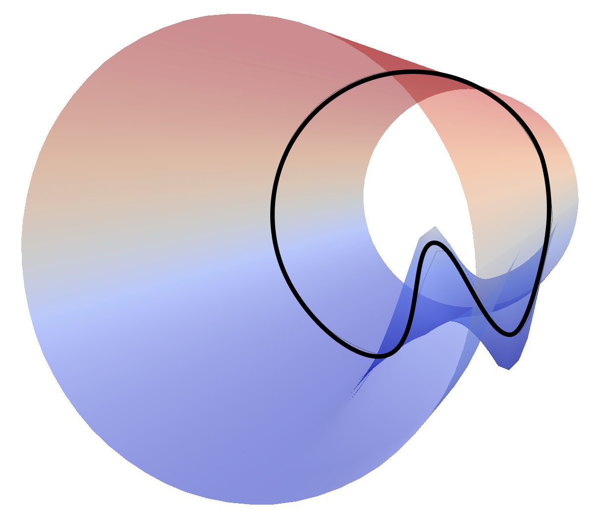
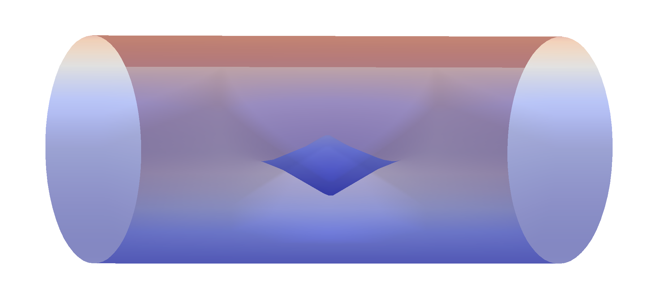
Figure 8: Left and middle: The wrinkled cylinder from two different angles. The left graphic contains the image of $\tilde{f}_{t}$ for some $t\in(p,q)$, a wrinkled circle, which has four critical points. Right: The Cerf diagram for the wrinkled cylinder.

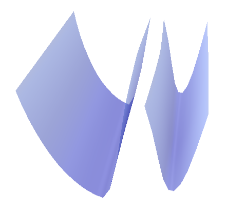
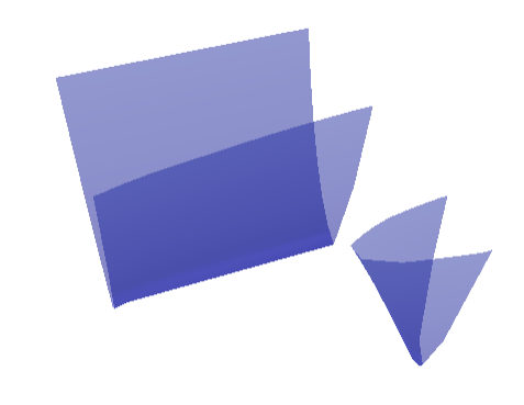
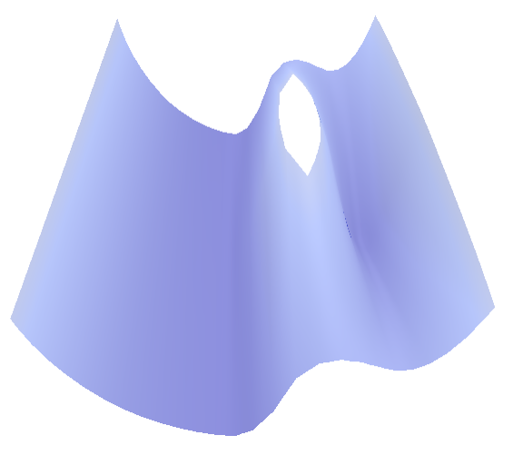
Figure 9: Left, middle, right: three cases of the semi-infinite strip $[a,b]\times(-\infty,c]$ are shown in blue overlaid on the Cerf diagram from Figure 9. The corresponding spaces $F(a,b,c)$ are shown to the right of each.

To aid in visualization of the persistence module, we again linearize the wrinkle (see the comment at the beginning Section 4). In Figure 10, the blue regions correspond to $H_{0}F$ and the red regions correspond to $H_{1}F$. Both $H_{0}F$ and $H_{1}F$ contain an unbounded region, arising from the global maxima and minima (fold) singularities, and a finite region, due to the wrinkle. Note that both $H_{0}F$ and $H_{1}F$ decompose into one-dimensional persistence modules, in contrast to the persistence modules of Theorem 4.1.

For precise formulas, assume $p=\frac{1}{4}$, $q=\frac{3}{4}$. Then the bounded component of $H_{1}F$ has support $m\leq c<n$, $0\leq a\leq\frac{1}{2}-\frac{1}{4}\frac{n-c}{n-m}$, and $\frac{1}{2}+\frac{1}{4}\frac{n-c}{n-m}\leq b\leq 1$. The bounded component of $H_{0}F$ has support given by the union of (i) $\ell\leq c<m$, $0\leq a\leq\frac{1}{2}+\frac{1}{4}\frac{c-\ell}{m-\ell}$, $\frac{1}{2}-\frac{1}{4}\frac{c-\ell}{m-\ell}\leq b\leq 1$, and (ii) $m\leq c<n$, $\frac{1}{2}-\frac{1}{4}\frac{n-c}{n-m}<a\leq b<\frac{1}{2}+\frac{1}{4}\frac{n-c}{n-m}$.

Figure 10: The persistence module for the wrinkled cylinder. Both $H_{0}F$ (blue) and $H_{1}F$ (red) decompose into two one-dimensional persistence modules, one bounded and one unbounded, in which all non-trivial maps are the identity map. The unbounded components, $0\leq a\leq b\leq 1$ together with $c\geq u$ and $c\geq v$, respectively, are exactly the persistence modules of the cylinder (Figure 6). The bounded components are due to the wrinkle.

Acknowledgments

This material is based upon work supported by, or in part by, the Army Research Laboratory and the Army Research Office under contract/grant number W911NF-18-1-0307.

References

- [1] Maciej Borodzik, András Némethi and Andrew Ranicki “Morse theory for manifolds with boundary” In Algebraic & Geometric Topology 16.2 Mathematical Sciences Publishers, 2016, pp. 971–1023
- [2] Dietrich Braess “Morse-Theorie für berandete Mannigfaltigkeiten” In Mathematische Annalen 208, 1974, pp. 133–148 URL: https://mathscinet.ams.org/mathscinet-getitem?mr=0348790
- [3] Peter Bubenik and Nikola Milićević “Homological Algebra for Persistence Modules” In Foundations of Computational Mathematics 21.5, 2021, pp. 1233–1278
- [4] Peter Bubenik, Jonathan Scott and Donald Stanley “Exact weights, path metrics, and algebraic Wasserstein distances” arXiv:1809.09654 In arXiv:1809.09654 [math.RA], 2018 URL: http://arxiv.org/abs/1809.09654
- [5] Peter Bubenik, Vin Silva and Jonathan Scott “Metrics for Generalized Persistence Modules” In Found. Comput. Math. 15.6, 2015, pp. 1501–1531
- [6] Ryan Budney and Tomasz Kaczynski “Bi-filtrations and persistence paths for 2-Morse functions” arXiv: 2110.08227 In arXiv:2110.08227 [math], 2021 URL: http://arxiv.org/abs/2110.08227
- [7] Gunnar Carlsson “Topology and data” In Bull. Amer. Math. Soc. (N.S.) 46.2, 2009, pp. 255–308
- [8] Gunnar Carlsson and Afra Zomorodian “The Theory of Multidimensional Persistence” In Discrete & Computational Geometry 42.1, 2009, pp. 71–93
- [9] Jean Cerf “La stratification naturelle des espaces de fonctions différentiables réelles et le théorème de la pseudo-isotopie” In Inst. Hautes Études Sci. Publ. Math., 1970, pp. 5–173
- [10] René Corbet, Ulderico Fugacci, Michael Kerber, Claudia Landi and Bei Wang “A kernel for multi-parameter persistent homology” In Computers & Graphics: X 2, 2019, pp. 100005
- [11] Y. M. Eliashberg and N. M. Mishachev “Wrinkling of smooth mappings and its applications. I” In Inventiones mathematicae 130.2, 1997, pp. 345–369
- [12] Robert Ghrist “Barcodes: the persistent topology of data” In Bull. Amer. Math. Soc. (N.S.) 45.1, 2008, pp. 61–75
- [13] Ryan E. Grady and Anna Schenfisch “Natural Stratifications of Reeb Spaces and Higher Morse Functions” In arXiv:2011.08404 [cs, math], 2020 URL: http://arxiv.org/abs/2011.08404
- [14] B. Hajduk “Minimal m-functions” In Fundamenta Mathematicae 111, 1981, pp. 179–200
- [15] Heather A. Harrington, Nina Otter, Hal Schenck and Ulrike Tillmann “Stratifying Multiparameter Persistent Homology” In SIAM Journal on Applied Algebra and Geometry 3.3, 2019, pp. 439–471
- [16] Allen Hatcher and John Wagoner “Pseudo-isotopies of compact manifolds” Astérisque, No. 6 Société Mathématique de France, Paris, 1973, pp. i+275
- [17] Kiyoshi Igusa “The space of framed functions” In Trans. Amer. Math. Soc. 301.2, 1987, pp. 431–477
- [18] M. C. Irwin “On the Stable Manifold Theorem” In Bulletin of the London Mathematical Society 2.2, 1970, pp. 196–198
- [19] A. Jankowski and R. Rubinsztein “Functions with non-degenerate critical points on manifolds with boundary” In Comment. Math. Prace Mat. 16, 1972, pp. 99–112
- [20] A Jankowski and R Rubinsztein “Functions with non-degenerate critical points on manifolds with boundary” In Comm. Math 16, 1972, pp. 99–112
- [21] Dominic Joyce “On manifolds with corners” Available arXiv: 0910.3518 In Advances in Geometric Analysis, Advanced Lectures in Mathematics 21 International Press, Boston, 2012, pp. 225–228
- [22] Mishal Assif P. K and Yuliy Baryshnikov “Biparametric persistence for smooth filtrations” In arXiv:2110.09602 [math], 2021 URL: http://arxiv.org/abs/2110.09602
- [23] Michael Kerber, Michael Lesnick and Steve Oudot “Exact computation of the matching distance on 2-parameter persistence modules” In J. Comput. Geom. 11.2, 2020, pp. 4–25
- [24] Robion Kirby “A Calculus for Framed Links in S3.” In Inventiones mathematicae 45, 1978, pp. 35–56
- [25] Michael Lesnick and Matthew Wright “Interactive Visualization of 2-D Persistence Modules” arXiv:1512.00180 [math.AT], 2015
- [26] Robert MacPherson and Amit Patel “Persistent local systems” In Adv. Math. 386, 2021, pp. 107795
- [27] Ezra Miller “Homological algebra of modules over posets” arXiv:2008.00063 [math.AT], 2020
- [28] J. Milnor “Morse theory” Princeton University Press, Princeton, N.J., 1963
- [29] Marston Morse “Relations between the critical points of a real function of independent variables” In Trans. Amer. Math. Soc. 27.3, 1925, pp. 345–396
- [30] Oliver Vipond “Multiparameter Persistence Landscapes” In Journal of Machine Learning Research 21.61, 2020, pp. 1–38