Search for high-energy neutrino sources from the direction of IceCube alert events

Abstract

We use IceCube’s high-statistics, neutrino-induced, through-going muon samples to search for astrophysical neutrino sources. Specifically, we analyze the arrival directions of IceCube’s highest energy neutrinos. These high-energy events allow for a good angular reconstruction of their origin. Additionally, they have a high probability to come from an astrophysical source. On average, 8 neutrino events that satisfy these selection criteria are detected per year. Using these neutrino events as a source catalog, we present a search for the production sites of cosmic neutrinos. In this contribution we explore a time-dependent analysis, and present preliminary 3$\sigma$ discovery potential fluences of $\approx 2.7\cdot 10^{-2}\rm{GeV}/\rm{cm}^{2}$. We construct the fluences using expectation maximization.

Corresponding authors: Martina Karl^1,2∗, Philipp Eller², Anna Schubert^2
1 Max Planck Institute for Physics, Föhringer Ring 6, 80805 München, Germany
² Technical University of Munich, James-Frank-Str. 1, 85748 Garching, Germany
^∗ Presenter

1 Introduction

The IceCube Neutrino Observatory [1] is a cubic-kilometer scale neutrino detector instrumenting a gigaton of ice at the geographic South Pole in Antarctica. Contrary to traditional telescopes, IceCube’s field of view comprises the whole sky with the greatest sensitivity for high-energy events at the horizon. It is thus ideally suited to inform other telescopes of interesting events. If a neutrino event has a high probability to be of astrophysical origin, IceCube sends alerts to other telescopes [2]. These notifications trigger follow-up multi-messenger observations [3]. A map of the arrival directions of IceCube alerts is shown in fig. 1. This map shows all events that fulfill the alert criteria [2], starting from August 2009, until March 2019.

On the 22nd of September 2017, IceCube detected an astrophysical neutrino (IceCube-170922A) with an extremely high energy (EHE alert). The promptly triggered gamma-ray follow-up observations detected a flaring blazar at the origin of this event [4]. Additionally, we searched for previous neutrino emission from the origin direction in archival IceCube data. We identified a neutrino flare from the same direction between September 2014 and March 2015 [5].

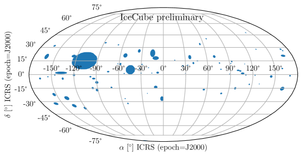
Figure 1: Sky map with the arrival directions of events fulfilling the IceCube alert criteria from August 2009 until March 2019. The size of a dot represents the uncertainty region of the reconstruction, providing a 90% chance of the alert to be from inside the filled region. Figure taken from [6].

This discovery leads to the question whether there are additional neutrino emissions coming from the origins of other alert events. To address this, we analyze 12 years of archival IceCube data and search for an excess in neutrino emission. The IceCube alerts provide positions of interest, comparable to a catalog of possible neutrino sources. A search for steady neutrino sources at the position of alert events was presented in [6]. In this specific analysis, we search for transient neutrino sources.

2 Analysis Method

We expand the time integrated analysis method (presented in [6]) with a time dependency. We use an unbinned likelihood approach.

2.1 Point source search with unbinned likelihood ratio

We expect two components in the neutrino-induced muon sample. One is the astrophysical signal, the other component is the atmospheric background [7]. Thus, the likelihood is a superposition of the signal ($S$) and background ($B$) probability density functions (pdfs). It is constructed by the product over all events $i$ in the sample. We can neglect the Poisson dependence due to the high number of events in the sample:

$$\mathcal{L}=\prod_{i}\left[\frac{n_{s}}{N}S_{i}(\vec{x}_{i},\sigma_{i},E_{i};\vec{x}_{s},\gamma,t_{i},t_{s})+\left(1-\frac{n_{s}}{N}\right)B_{i}(\delta_{i},E_{i},livetime)\right].$$ (1)

Here, $n_{s}$ denotes the mean number of expected signal events in the detector and is divided by $N$, which is the total number of all detected events (background + signal). The reconstructed origin position for each event $i$ is $\vec{x}_{i}=(\alpha_{i},\delta_{i})$, the right ascension $\alpha$ and the declination $\delta$. The one sigma uncertainty of this reconstructed position is given with $\sigma_{i}$. The event’s energy is given as $E_{i}$, and the time the event was detected is given as $t_{i}$. We also consider the source properties: the source position $\vec{x}_{s}$, and the source energy spectral index $\gamma$. We assume a power law emission spectrum of $\propto E^{-\gamma}$. The source has a time dependency, which is denoted as $t_{s}$ in the form of flaring time and flare duration. The total detector up-time of the considered data period is called $livetime$. The signal pdf $S_{i}$ can be split into different parts $S(\vec{x}_{i},\sigma_{i},E_{i};\vec{x}_{s},\gamma,t_{i},t_{s})=S_{spatial}\cdot S_{energy}\cdot S_{temporal}$ [7]:

$$S_{spatial}\cdot S_{energy}=S_{i}(\vec{x}_{i},\sigma_{i};\vec{x}_{s})\cdot\varepsilon_{s}(E_{i};\delta_{i},\gamma)=\frac{1}{2\pi\sigma_{i}^{2}}\exp\left(-\frac{|\vec{x}_{i}-\vec{x}_{s}|^{2}}{2\sigma_{i}^{2}}\right)\cdot\varepsilon_{s}(E_{i};\delta_{i},\gamma),$$ (2)

$$S_{temporal}(t_{i},\mu_{T},\sigma_{T})=\frac{1}{{\sigma_{T}\sqrt{2\pi}}}e^{{{-\left({t_{i}-\mu_{T}}\right)^{2}}\mathord{\left/{\vphantom{{-\left({t_{i}-\mu_{T}}\right)^{2}}{2\sigma_{T}^{2}}}}\right.\kern-1.2pt}{2\sigma_{T}^{2}}}}.$$ (3)

The spatial part shows a Gaussian distribution with the source position as mean and the event reconstruction uncertainty as standard deviation. We take the uncertainty of the source position into account in section 2.2. The energy factor $\varepsilon_{s}$ is the probability density function for a signal event of energy $E_{i}$ depending on its declination $\delta_{i}$, and the source spectral index $\gamma$. This factor is calculated from Monte Carlo simulation [7]. In the time pdf, we assume that neutrino flares are emitted in a Gaussian shape with the mean $\mu_{T}$ and the standard deviation $\sigma_{T}$.

Similarly, we express the background pdf $B_{i}$ as $B(\vec{x}_{i},E_{i},livetime)=B_{spatial}\cdot B_{energy}\cdot B_{temporal}$ [7]:

$$B\left(\vec{x}_{i},E_{i},livetime\right)=B_{i}(\vec{x}_{i})\cdot\varepsilon_{B}(E_{i};\delta_{i})\cdot B(livetime)=\frac{1}{2\pi}\cdot P(\delta_{i})\cdot\varepsilon_{B}(E_{i};\delta_{i})\cdot\frac{1}{livetime},$$ (4)

because of Icecube’s unique geographic location and symmetry, we can assume uniformity over right ascension for background events. The spatial background pdf depends only on declination $\delta_{i}$, because of detector geometry. Here, similar to the signal case, the energy term $\varepsilon_{B}$ denotes the probability density function for a background event with energy $E_{i}$ at declination $\delta_{i}$. In the temporal background we assume a uniform distribution over the whole detector up-time of IceCube ($livetime$).

We take the likelihood ratio of the null-hypothesis (background only, $n_{s}=0$) and the best fit of the signal hypothesis $n_{s}>0$ to calculate the test statistics (TS). We also need to consider the look-elsewhere effect, since there are more short time flare windows than long time flare windows. We correct this by introducing a penalty factor ($pf$) [7]. The penalty factor depends on the maximum allowed flare length, which is 300 days. The test statistics can be expressed as follows [7]:

$$\begin{split}TS=2\left(\log\left[\frac{P(Data|H_{S})}{P(Data|H_{0})}\right]-\log\left(pf\right)\right)&=2~{}\left(\sum_{i}\log\left[\frac{\hat{n}_{s}}{N_{obs}}\left(\frac{S_{i}}{B_{i}}-1\right)+1\right]-\log\left(\frac{300~{}\rm{days}}{\sqrt{2\pi}\sigma_{T}}\right)\right).\end{split}$$ (5)

2.2 Position fit

We consider alert events in IceCube to be a source catalog for potential high-energy neutrino sources. The alerts do not provide a precise, point-like position of sources. The 90% error regions are shown in fig. 1. We are looking for point-like sources within the 90% reconstructed uncertainty region of alerts. For this, we divide the uncertainty region in an evenly spaced grid of $0.1^{\circ}$ in right ascension and declination. This grid size is smaller than the reconstruction angular resolution, thus this method represents an unbinned search. At each point, we fit the maximal test statistic value depending on the mean number of signal events and the source energy spectral index. Eventually, we select the point yielding the highest test statistic value as the source position. This approach was also used in [6]. We illustrate this procedure in figure 2. With this best test statistic value, we build the test statistic distribution and determine a p-value for each alert.

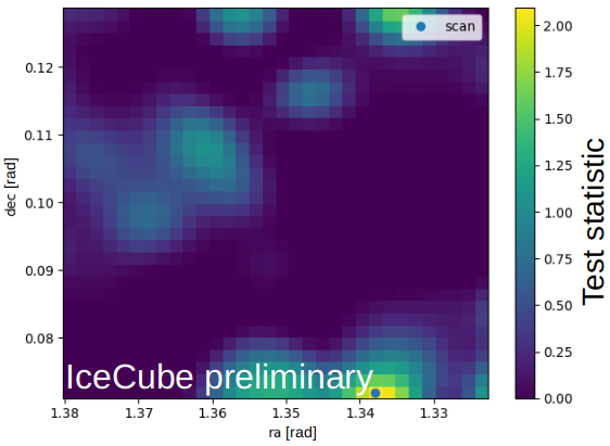
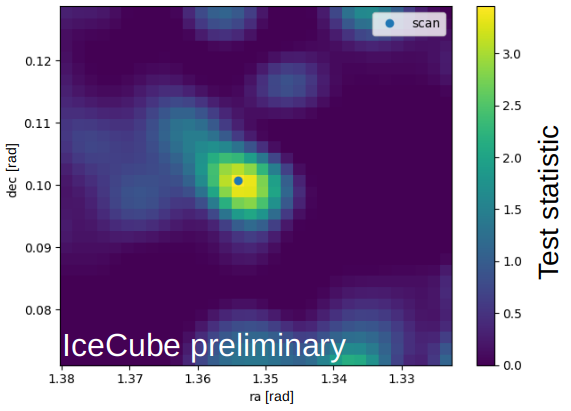
Figure 2: We show example plots of a reconstructed alert 90% uncertainty region, the test statistic values for a random background distribution (left) and a region with injected signal (right). We divide each region into steps with $0.1^{\circ}$ spacing. We determine the best test statistic value at each step by fitting the best mean number of signal events and energy spectral index. We consider the position with the highest test statistic value as the point source position, indicated with the blue dot ("scan"). In the left plot the scan finds the position with the most significant background fluctuation. In the right plot, we simulate 10 signal events injected at the center of the region. The scan returns the position with the simulated signal. Figure taken from [6].

2.3 Search for neutrino flares

At each point in the position grid, we search the data for possible time-dependent neutrino flares. Previous approaches followed a brute force testing of different neutrino flares [5]. If we combine the brute force flare search with the brute force position search (see previous paragraph 2.2), we need prohibitively large computational resources for calculation of the test statistic. Thus, we apply a new method for the search for neutrino flares in IceCube data: we use expectation maximization [8] (EM), an unsupervised learning algorithm. This new approach speeds up the analysis significantly (about a factor of $10000$). An in-depth explanation of the expectation maximization algorithm can be found in [9].

We use a mixture model, with a Gaussian signal pdf (the neutrino flare in time) and a uniform background distribution. We take the spatial and energy information as our data and want to determine the flaring time. We use the spatial and energy signal pdf over background pdf ratio $SoB=\frac{S_{spatial}\cdot S_{energy}}{B_{spatial}\cdot B_{energy}}$, with each pdf defined as in equations 2 and 4. Then we apply the EM algorithm with the mixture model on the $SoB$ over time distribution. Hence, we find the best fitting Gaussian time pdf for events that are close to the source and could follow the source spectral distribution. We show an example of the EM algorithm in fig. 3. Left we see the $SoB$ distribution vs. time for background data only and the best fit of background fluctuations. On the right we simulated a neutrino flare of 10 events within 110 days. Their $SoB$ values exceed the background $SoB$ by some orders of magnitude because of their spatial clustering and higher energies. The EM algorithm then maximizes the likelihood and determines the best flaring time. We can then calculate the temporal pdf and determine the test statistic value as in eq. 5. We repeat this procedure at every grid point in the uncertainty area (see section 2.2).

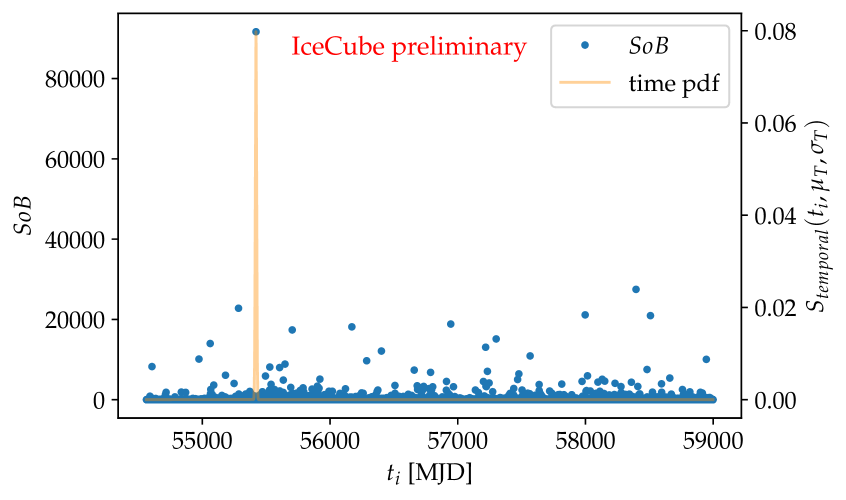
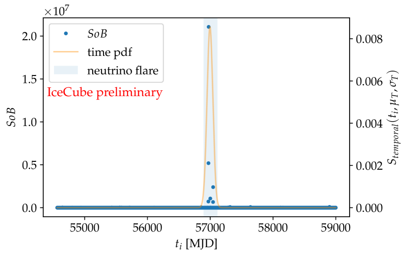
Figure 3: Left: The $SoB$ ratios for background. The EM algorithm fits background fluctuations (orange curve).
Right: We simulate a neutrino flare of 10 events within 110 days (blue shaded region), the $SoB$ values of these events exceed the background $SoB$ by some orders of magnitude. The EM algorithm finds the flare and determines proper parameters ($\mu_{T},\sigma_{T}$) for the time pdf (orange Gaussian curve).

2.4 Parametrized description of the test statistic quantiles depending on flare parameter

The search for a clustering in time in addition to a clustering in space means highly increased computational effort. We investigate an analytical description of how the test statistic distribution changes for different flare intensities.

In this test, we specifically want to investigate the effect of the flare itself. We eliminate other influences by assuming we know the correct position and the correct flare parameters. We also consider a box-shaped neutrino flare model. The box-shaped pdf allows only neutrino emission between the flare starting time $t_{start}$ and the flare end time $t_{end}$. The temporal signal pdf is thus 0 for $t_{i}\notin[t_{start},t_{end}]$ and $\frac{1}{\Delta t}$ for $t_{i}\in[t_{start},t_{end}$], where $\Delta t=t_{end}-t_{start}$.

We use this time pdf in equation 5. We find the dependency $TS\propto\log\left(\frac{n_{s}}{\Delta t}\right)$ and define the fitting function:

$$TS\propto a+b\cdot\text{log}\left(\frac{n_{s}}{\Delta t}\right).$$ (6)

We simulate different flare strengths and flare durations and calculate the test statistic median for each flare (see fig. 4). For a fixed flare strength, we fit the test statistic median with the logarithmic function in eq. 6, shown in the left of fig. 5. The parameters $a$ and $b$ show a linear dependency on the flare strength (see right of fig. 5). With this, we can analytically sample the test statistic quantiles for different flares.

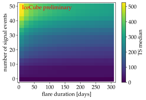
Figure 4: The test statistic median for different flares. We simulated flares with a duration of up to 300 days (x-axis) and with a signal strengths of up to 50 neutrinos (y-axis). Short strong flares yield very high test statistic values, which decrease with increasing flaring time or weaker flare strength.

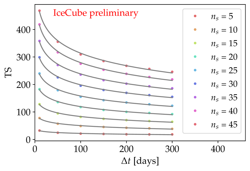
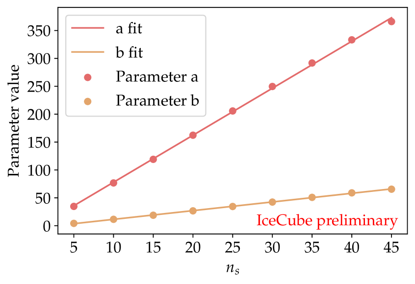
Figure 5: Left: the points show the simulated test statistic median for different fixed number of signal events (ninj). The black line is the fit with the function $TS=a+b\cdot\text{log}\left(\frac{n}{\Delta t}\right)$. For each flare strength, the fit accurately describes how the test statistic median changes with increasing flare duration.
Right: We take the parameters $a$ and $b$ of the fitting function $TS=a+b\cdot\text{log}\left(\frac{n}{\Delta t}\right)$. The fit paramaters show a linear dependency on the flare strength.

3 Performance study

We examine the performance of the analysis. A measure for this is the discovery potential. The $3\sigma$ discovery potential is defined as the source flux for which we have a 50% chance to determine a p-value of at least $3\sigma$.

In the time-dependent case, a relevant quantity is the total neutrino emission seen from the source during the neutrino flare – the fluence. The fluence is the source flux integrated over flaring time. We present the $3\sigma$ discovery potential fluences of this analysis at the position of the blazar TXS0506+056 ($\alpha=77.366^{\circ},\delta=5.69^{\circ}$) and for the same flare duration as discovered in [5] ($\sigma_{T}=55.18~{}\rm{days},\Delta t=110.36~{}\rm{days}$). We assume a source spectral index of $\gamma=2$.

We combine several data sets from different data taking periods of IceCube. We want to determine the overall $3\sigma$ discovery potential fluence. Additionally, we want to find out whether these different data sets influence which source flux we can potentially detect. Thus we simulate similar neutrino flares in each data sample and evaluate the fluence of the respective $3\sigma$ discovery potential. We also compare how the shape of the time pdf influences the $3\sigma$ discovery potential fluence. For this, we additionally simulate a neutrino flare following a box-shaped time pdf (as described in section 2.4).

In table 1, we show the $3\sigma$ discovery potential fluence for each data taking period. We see a slight difference in fluences for different data samples. We calculate the $3\sigma$ discovery potential fluence for a box-shaped time pdf for the latest and longest data set. The fluence for the box-shaped pdf agrees with the fluence of the Gaussian time pdf (see the last two lines of table 1). The mean $3\sigma$ discovery potential fluence is $2.7\cdot 10^{-2}\rm{GeV}/\rm{cm}^{2}$.

Time pdf shape	Duration of data taking period [days]	$3\sigma$ discovery potential fluence [$\frac{\rm{GeV}}{\rm{cm}^{2}}$]
Gaussian	409	0.027
Gaussian	376	0.037
Gaussian	346	0.032
Gaussian	3304	0.026
Box	3304	0.026

Table 1: The $3\sigma$ discovery potential fluences for different data sets, time pdfs (first row), and data sets (second row). The second row lists the duration of the IceCube data taking period within the respective data set. We compare the fluences for a Gaussian time pdf with the fluence for a box-shaped time pdf for a flare in the latest data set (last two lines). We find that the fluence does not depend on the shape of the time pdf.

4 Conclusion

We search for transient neutrino sources in 12 years of IceCube archival data. We present improved methods for a time-dependent point source analysis. With expectation maximization we use a fast and efficient flare finding method. We also explore methods to analytically describe how the test statistic quantiles change for different flare intensities. We determine $3\sigma$ discovery potential fluences in the range of $\approx 2.7\cdot 10^{-2}\rm{GeV}/\rm{cm}^{2}$. With this analysis, we will be able set new upper fluence limits as soon as we run the analysis on unblinded IceCube data.

Full Author List: IceCube Collaboration

R. Abbasi¹⁷, M. Ackermann⁵⁹, J. Adams¹⁸, J. A. Aguilar¹², M. Ahlers²², M. Ahrens⁵⁰, C. Alispach²⁸, A. A. Alves Jr.³¹, N. M. Amin⁴², R. An¹⁴, K. Andeen⁴⁰, T. Anderson⁵⁶, G. Anton²⁶, C. Argüelles¹⁴, Y. Ashida³⁸, S. Axani¹⁵, X. Bai⁴⁶, A. Balagopal V.³⁸, A. Barbano²⁸, S. W. Barwick³⁰, B. Bastian⁵⁹, V. Basu³⁸, S. Baur¹², R. Bay⁸, J. J. Beatty^20, 21, K.-H. Becker⁵⁸, J. Becker Tjus¹¹, C. Bellenghi²⁷, S. BenZvi⁴⁸, D. Berley¹⁹, E. Bernardini^59, 60, D. Z. Besson^34, 61, G. Binder^8, 9, D. Bindig⁵⁸, E. Blaufuss¹⁹, S. Blot⁵⁹, M. Boddenberg¹, F. Bontempo³¹, J. Borowka¹, S. Böser³⁹, O. Botner⁵⁷, J. Böttcher¹, E. Bourbeau²², F. Bradascio⁵⁹, J. Braun³⁸, S. Bron²⁸, J. Brostean-Kaiser⁵⁹, S. Browne³², A. Burgman⁵⁷, R. T. Burley², R. S. Busse⁴¹, M. A. Campana⁴⁵, E. G. Carnie-Bronca², C. Chen⁶, D. Chirkin³⁸, K. Choi⁵², B. A. Clark²⁴, K. Clark³³, L. Classen⁴¹, A. Coleman⁴², G. H. Collin¹⁵, J. M. Conrad¹⁵, P. Coppin¹³, P. Correa¹³, D. F. Cowen^55, 56, R. Cross⁴⁸, C. Dappen¹, P. Dave⁶, C. De Clercq¹³, J. J. DeLaunay⁵⁶, H. Dembinski⁴², K. Deoskar⁵⁰, S. De Ridder²⁹, A. Desai³⁸, P. Desiati³⁸, K. D. de Vries¹³, G. de Wasseige¹³, M. de With¹⁰, T. DeYoung²⁴, S. Dharani¹, A. Diaz¹⁵, J. C. Díaz-Vélez³⁸, M. Dittmer⁴¹, H. Dujmovic³¹, M. Dunkman⁵⁶, M. A. DuVernois³⁸, E. Dvorak⁴⁶, T. Ehrhardt³⁹, P. Eller²⁷, R. Engel^31, 32, H. Erpenbeck¹, J. Evans¹⁹, P. A. Evenson⁴², K. L. Fan¹⁹, A. R. Fazely⁷, S. Fiedlschuster²⁶, A. T. Fienberg⁵⁶, K. Filimonov⁸, C. Finley⁵⁰, L. Fischer⁵⁹, D. Fox⁵⁵, A. Franckowiak^11, 59, E. Friedman¹⁹, A. Fritz³⁹, P. Fürst¹, T. K. Gaisser⁴², J. Gallagher³⁷, E. Ganster¹, A. Garcia¹⁴, S. Garrappa⁵⁹, L. Gerhardt⁹, A. Ghadimi⁵⁴, C. Glaser⁵⁷, T. Glauch²⁷, T. Glüsenkamp²⁶, A. Goldschmidt⁹, J. G. Gonzalez⁴², S. Goswami⁵⁴, D. Grant²⁴, T. Grégoire⁵⁶, S. Griswold⁴⁸, M. Gündüz¹¹, C. Günther¹, C. Haack²⁷, A. Hallgren⁵⁷, R. Halliday²⁴, L. Halve¹, F. Halzen³⁸, M. Ha Minh²⁷, K. Hanson³⁸, J. Hardin³⁸, A. A. Harnisch²⁴, A. Haungs³¹, S. Hauser¹, D. Hebecker¹⁰, K. Helbing⁵⁸, F. Henningsen²⁷, E. C. Hettinger²⁴, S. Hickford⁵⁸, J. Hignight²⁵, C. Hill¹⁶, G. C. Hill², K. D. Hoffman¹⁹, R. Hoffmann⁵⁸, T. Hoinka²³, B. Hokanson-Fasig³⁸, K. Hoshina^38, 62, F. Huang⁵⁶, M. Huber²⁷, T. Huber³¹, K. Hultqvist⁵⁰, M. Hünnefeld²³, R. Hussain³⁸, S. In⁵², N. Iovine¹², A. Ishihara¹⁶, M. Jansson⁵⁰, G. S. Japaridze⁵, M. Jeong⁵², B. J. P. Jones⁴, D. Kang³¹, W. Kang⁵², X. Kang⁴⁵, A. Kappes⁴¹, D. Kappesser³⁹, T. Karg⁵⁹, M. Karl²⁷, A. Karle³⁸, U. Katz²⁶, M. Kauer³⁸, M. Kellermann¹, J. L. Kelley³⁸, A. Kheirandish⁵⁶, K. Kin¹⁶, T. Kintscher⁵⁹, J. Kiryluk⁵¹, S. R. Klein^8, 9, R. Koirala⁴², H. Kolanoski¹⁰, T. Kontrimas²⁷, L. Köpke³⁹, C. Kopper²⁴, S. Kopper⁵⁴, D. J. Koskinen²², P. Koundal³¹, M. Kovacevich⁴⁵, M. Kowalski^10, 59, T. Kozynets²², E. Kun¹¹, N. Kurahashi⁴⁵, N. Lad⁵⁹, C. Lagunas Gualda⁵⁹, J. L. Lanfranchi⁵⁶, M. J. Larson¹⁹, F. Lauber⁵⁸, J. P. Lazar^14, 38, J. W. Lee⁵², K. Leonard³⁸, A. Leszczyńska³², Y. Li⁵⁶, M. Lincetto¹¹, Q. R. Liu³⁸, M. Liubarska²⁵, E. Lohfink³⁹, C. J. Lozano Mariscal⁴¹, L. Lu³⁸, F. Lucarelli²⁸, A. Ludwig^24, 35, W. Luszczak³⁸, Y. Lyu^8, 9, W. Y. Ma⁵⁹, J. Madsen³⁸, K. B. M. Mahn²⁴, Y. Makino³⁸, S. Mancina³⁸, I. C. Mariş¹², R. Maruyama⁴³, K. Mase¹⁶, T. McElroy²⁵, F. McNally³⁶, J. V. Mead²², K. Meagher³⁸, A. Medina²¹, M. Meier¹⁶, S. Meighen-Berger²⁷, J. Micallef²⁴, D. Mockler¹², T. Montaruli²⁸, R. W. Moore²⁵, R. Morse³⁸, M. Moulai¹⁵, R. Naab⁵⁹, R. Nagai¹⁶, U. Naumann⁵⁸, J. Necker⁵⁹, L. V. Nguyễn²⁴, H. Niederhausen²⁷, M. U. Nisa²⁴, S. C. Nowicki²⁴, D. R. Nygren⁹, A. Obertacke Pollmann⁵⁸, M. Oehler³¹, A. Olivas¹⁹, E. O’Sullivan⁵⁷, H. Pandya⁴², D. V. Pankova⁵⁶, N. Park³³, G. K. Parker⁴, E. N. Paudel⁴², L. Paul⁴⁰, C. Pérez de los Heros⁵⁷, L. Peters¹, J. Peterson³⁸, S. Philippen¹, D. Pieloth²³, S. Pieper⁵⁸, M. Pittermann³², A. Pizzuto³⁸, M. Plum⁴⁰, Y. Popovych³⁹, A. Porcelli²⁹, M. Prado Rodriguez³⁸, P. B. Price⁸, B. Pries²⁴, G. T. Przybylski⁹, C. Raab¹², A. Raissi¹⁸, M. Rameez²², K. Rawlins³, I. C. Rea²⁷, A. Rehman⁴², P. Reichherzer¹¹, R. Reimann¹, G. Renzi¹², E. Resconi²⁷, S. Reusch⁵⁹, W. Rhode²³, M. Richman⁴⁵, B. Riedel³⁸, E. J. Roberts², S. Robertson^8, 9, G. Roellinghoff⁵², M. Rongen³⁹, C. Rott^49, 52, T. Ruhe²³, D. Ryckbosch²⁹, D. Rysewyk Cantu²⁴, I. Safa^14, 38, J. Saffer³², S. E. Sanchez Herrera²⁴, A. Sandrock²³, J. Sandroos³⁹, M. Santander⁵⁴, S. Sarkar⁴⁴, S. Sarkar²⁵, K. Satalecka⁵⁹, M. Scharf¹, M. Schaufel¹, H. Schieler³¹, S. Schindler²⁶, P. Schlunder²³, T. Schmidt¹⁹, A. Schneider³⁸, J. Schneider²⁶, F. G. Schröder^31, 42, L. Schumacher²⁷, G. Schwefer¹, S. Sclafani⁴⁵, D. Seckel⁴², S. Seunarine⁴⁷, A. Sharma⁵⁷, S. Shefali³², M. Silva³⁸, B. Skrzypek¹⁴, B. Smithers⁴, R. Snihur³⁸, J. Soedingrekso²³, D. Soldin⁴², C. Spannfellner²⁷, G. M. Spiczak⁴⁷, C. Spiering^59, 61, J. Stachurska⁵⁹, M. Stamatikos²¹, T. Stanev⁴², R. Stein⁵⁹, J. Stettner¹, A. Steuer³⁹, T. Stezelberger⁹, T. Stürwald⁵⁸, T. Stuttard²², G. W. Sullivan¹⁹, I. Taboada⁶, F. Tenholt¹¹, S. Ter-Antonyan⁷, S. Tilav⁴², F. Tischbein¹, K. Tollefson²⁴, L. Tomankova¹¹, C. Tönnis⁵³, S. Toscano¹², D. Tosi³⁸, A. Trettin⁵⁹, M. Tselengidou²⁶, C. F. Tung⁶, A. Turcati²⁷, R. Turcotte³¹, C. F. Turley⁵⁶, J. P. Twagirayezu²⁴, B. Ty³⁸, M. A. Unland Elorrieta⁴¹, N. Valtonen-Mattila⁵⁷, J. Vandenbroucke³⁸, N. van Eijndhoven¹³, D. Vannerom¹⁵, J. van Santen⁵⁹, S. Verpoest²⁹, M. Vraeghe²⁹, C. Walck⁵⁰, T. B. Watson⁴, C. Weaver²⁴, P. Weigel¹⁵, A. Weindl³¹, M. J. Weiss⁵⁶, J. Weldert³⁹, C. Wendt³⁸, J. Werthebach²³, M. Weyrauch³², N. Whitehorn^24, 35, C. H. Wiebusch¹, D. R. Williams⁵⁴, M. Wolf²⁷, K. Woschnagg⁸, G. Wrede²⁶, J. Wulff¹¹, X. W. Xu⁷, Y. Xu⁵¹, J. P. Yanez²⁵, S. Yoshida¹⁶, S. Yu²⁴, T. Yuan³⁸, Z. Zhang⁵¹

¹ III. Physikalisches Institut, RWTH Aachen University, D-52056 Aachen, Germany
² Department of Physics, University of Adelaide, Adelaide, 5005, Australia
³ Dept. of Physics and Astronomy, University of Alaska Anchorage, 3211 Providence Dr., Anchorage, AK 99508, USA
⁴ Dept. of Physics, University of Texas at Arlington, 502 Yates St., Science Hall Rm 108, Box 19059, Arlington, TX 76019, USA
⁵ CTSPS, Clark-Atlanta University, Atlanta, GA 30314, USA
⁶ School of Physics and Center for Relativistic Astrophysics, Georgia Institute of Technology, Atlanta, GA 30332, USA
⁷ Dept. of Physics, Southern University, Baton Rouge, LA 70813, USA
⁸ Dept. of Physics, University of California, Berkeley, CA 94720, USA
⁹ Lawrence Berkeley National Laboratory, Berkeley, CA 94720, USA
¹⁰ Institut für Physik, Humboldt-Universität zu Berlin, D-12489 Berlin, Germany
¹¹ Fakultät für Physik & Astronomie, Ruhr-Universität Bochum, D-44780 Bochum, Germany
¹² Université Libre de Bruxelles, Science Faculty CP230, B-1050 Brussels, Belgium
¹³ Vrije Universiteit Brussel (VUB), Dienst ELEM, B-1050 Brussels, Belgium
¹⁴ Department of Physics and Laboratory for Particle Physics and Cosmology, Harvard University, Cambridge, MA 02138, USA
¹⁵ Dept. of Physics, Massachusetts Institute of Technology, Cambridge, MA 02139, USA
¹⁶ Dept. of Physics and Institute for Global Prominent Research, Chiba University, Chiba 263-8522, Japan
¹⁷ Department of Physics, Loyola University Chicago, Chicago, IL 60660, USA
¹⁸ Dept. of Physics and Astronomy, University of Canterbury, Private Bag 4800, Christchurch, New Zealand
¹⁹ Dept. of Physics, University of Maryland, College Park, MD 20742, USA
²⁰ Dept. of Astronomy, Ohio State University, Columbus, OH 43210, USA
²¹ Dept. of Physics and Center for Cosmology and Astro-Particle Physics, Ohio State University, Columbus, OH 43210, USA
²² Niels Bohr Institute, University of Copenhagen, DK-2100 Copenhagen, Denmark
²³ Dept. of Physics, TU Dortmund University, D-44221 Dortmund, Germany
²⁴ Dept. of Physics and Astronomy, Michigan State University, East Lansing, MI 48824, USA
²⁵ Dept. of Physics, University of Alberta, Edmonton, Alberta, Canada T6G 2E1
²⁶ Erlangen Centre for Astroparticle Physics, Friedrich-Alexander-Universität Erlangen-Nürnberg, D-91058 Erlangen, Germany
²⁷ Physik-Department, Technische Universität München, D-85748 Garching, Germany
²⁸ Département de physique nucléaire et corpusculaire, Université de Genève, CH-1211 Genève, Switzerland
²⁹ Dept. of Physics and Astronomy, University of Gent, B-9000 Gent, Belgium
³⁰ Dept. of Physics and Astronomy, University of California, Irvine, CA 92697, USA
³¹ Karlsruhe Institute of Technology, Institute for Astroparticle Physics, D-76021 Karlsruhe, Germany
³² Karlsruhe Institute of Technology, Institute of Experimental Particle Physics, D-76021 Karlsruhe, Germany
³³ Dept. of Physics, Engineering Physics, and Astronomy, Queen’s University, Kingston, ON K7L 3N6, Canada
³⁴ Dept. of Physics and Astronomy, University of Kansas, Lawrence, KS 66045, USA
³⁵ Department of Physics and Astronomy, UCLA, Los Angeles, CA 90095, USA
³⁶ Department of Physics, Mercer University, Macon, GA 31207-0001, USA
³⁷ Dept. of Astronomy, University of Wisconsin–Madison, Madison, WI 53706, USA
³⁸ Dept. of Physics and Wisconsin IceCube Particle Astrophysics Center, University of Wisconsin–Madison, Madison, WI 53706, USA
³⁹ Institute of Physics, University of Mainz, Staudinger Weg 7, D-55099 Mainz, Germany
⁴⁰ Department of Physics, Marquette University, Milwaukee, WI, 53201, USA
⁴¹ Institut für Kernphysik, Westfälische Wilhelms-Universität Münster, D-48149 Münster, Germany
⁴² Bartol Research Institute and Dept. of Physics and Astronomy, University of Delaware, Newark, DE 19716, USA
⁴³ Dept. of Physics, Yale University, New Haven, CT 06520, USA
⁴⁴ Dept. of Physics, University of Oxford, Parks Road, Oxford OX1 3PU, UK
⁴⁵ Dept. of Physics, Drexel University, 3141 Chestnut Street, Philadelphia, PA 19104, USA
⁴⁶ Physics Department, South Dakota School of Mines and Technology, Rapid City, SD 57701, USA
⁴⁷ Dept. of Physics, University of Wisconsin, River Falls, WI 54022, USA
⁴⁸ Dept. of Physics and Astronomy, University of Rochester, Rochester, NY 14627, USA
⁴⁹ Department of Physics and Astronomy, University of Utah, Salt Lake City, UT 84112, USA
⁵⁰ Oskar Klein Centre and Dept. of Physics, Stockholm University, SE-10691 Stockholm, Sweden
⁵¹ Dept. of Physics and Astronomy, Stony Brook University, Stony Brook, NY 11794-3800, USA
⁵² Dept. of Physics, Sungkyunkwan University, Suwon 16419, Korea
⁵³ Institute of Basic Science, Sungkyunkwan University, Suwon 16419, Korea
⁵⁴ Dept. of Physics and Astronomy, University of Alabama, Tuscaloosa, AL 35487, USA
⁵⁵ Dept. of Astronomy and Astrophysics, Pennsylvania State University, University Park, PA 16802, USA
⁵⁶ Dept. of Physics, Pennsylvania State University, University Park, PA 16802, USA
⁵⁷ Dept. of Physics and Astronomy, Uppsala University, Box 516, S-75120 Uppsala, Sweden
⁵⁸ Dept. of Physics, University of Wuppertal, D-42119 Wuppertal, Germany
⁵⁹ DESY, D-15738 Zeuthen, Germany
⁶⁰ Università di Padova, I-35131 Padova, Italy
⁶¹ National Research Nuclear University, Moscow Engineering Physics Institute (MEPhI), Moscow 115409, Russia
⁶² Earthquake Research Institute, University of Tokyo, Bunkyo, Tokyo 113-0032, Japan

Acknowledgements

USA – U.S. National Science Foundation-Office of Polar Programs, U.S. National Science Foundation-Physics Division, U.S. National Science Foundation-EPSCoR, Wisconsin Alumni Research Foundation, Center for High Throughput Computing (CHTC) at the University of Wisconsin–Madison, Open Science Grid (OSG), Extreme Science and Engineering Discovery Environment (XSEDE), Frontera computing project at the Texas Advanced Computing Center, U.S. Department of Energy-National Energy Research Scientific Computing Center, Particle astrophysics research computing center at the University of Maryland, Institute for Cyber-Enabled Research at Michigan State University, and Astroparticle physics computational facility at Marquette University; Belgium – Funds for Scientific Research (FRS-FNRS and FWO), FWO Odysseus and Big Science programmes, and Belgian Federal Science Policy Office (Belspo); Germany – Bundesministerium für Bildung und Forschung (BMBF), Deutsche Forschungsgemeinschaft (DFG), Helmholtz Alliance for Astroparticle Physics (HAP), Initiative and Networking Fund of the Helmholtz Association, Deutsches Elektronen Synchrotron (DESY), and High Performance Computing cluster of the RWTH Aachen; Sweden – Swedish Research Council, Swedish Polar Research Secretariat, Swedish National Infrastructure for Computing (SNIC), and Knut and Alice Wallenberg Foundation; Australia – Australian Research Council; Canada – Natural Sciences and Engineering Research Council of Canada, Calcul Québec, Compute Ontario, Canada Foundation for Innovation, WestGrid, and Compute Canada; Denmark – Villum Fonden and Carlsberg Foundation; New Zealand – Marsden Fund; Japan – Japan Society for Promotion of Science (JSPS) and Institute for Global Prominent Research (IGPR) of Chiba University; Korea – National Research Foundation of Korea (NRF); Switzerland – Swiss National Science Foundation (SNSF); United Kingdom – Department of Physics, University of Oxford.

References

- [1] IceCube Collaboration, M. Aartsen et al. Journal of Instrumentation 12 no. 03, (2017) P03012–P03012.
- [2] IceCube Collaboration, M. G. Aartsen et al. Astropart. Phys. 92 (2017) 30–41.
- [3] Thomas Kintscher for the IceCube Collaboration Journal of Physics: Conference Series 718 (2016) 062029.
- [4] IceCube, Fermi-LAT, MAGIC, AGILE, ASAS-SN, HAWC, H.E.S.S, INTEGRAL, Kanata, Kiso, Kapteyn, Liverpool telescope, Subaru, Swift/NuSTAR, VERITAS, and VLA/17b-403 Collaboration, M. G. Aartsen et al. Science 361 (2018) eaat1378.
- [5] IceCube Collaboration, M. G. Aartsen et al. Science 361 (2018) 147–151.
- [6] M. Karl, “Search for Neutrino Emission in IceCube’s Archival Data from the Direction of IceCube Alert Events,” in 36th International Cosmic Ray Conference (ICRC2019), vol. 36 of International Cosmic Ray Conference, p. 929. July, 2019. arXiv:1908.05162 [astro-ph.HE].
- [7] J. Braun, J. Dumm, F. De Palma, C. Finley, A. Karle, and T. Montaruli Astropart. Phys. 29 (2008) 299–305.
- [8] A. P. Dempster, N. M. Laird, and D. B. Rubin Journal of the Royal Statistical Society. Series B (Methodological) 39 no. 1, (1977) 1–38.
- [9] W. Press, W. H, S. Teukolsky, W. Vetterling, S. A, and B. Flannery, Numerical Recipes 3rd Edition: The Art of Scientific Computing. Cambridge University Press, 2007. https://books.google.de/books?id=1aAOdzK3FegC.