TIFR/TH/21-1

We make a careful re-examination of the possibility that, in a $U(1)$ extension of the Standard Model, the extra $Z^{\prime}$ boson may acquire a mass from a Stückelberg-type scalar. The model, when all issues of theoretical consistency are taken into account, contains several attractive new features, including a high degree of predictability.

PACS Nos: 12.15.-y, 12.60.-i, 14.80.-j

 

1 Introduction

In recent times, it has become something of a cliché that physics beyond the Standard Model (SM) of elementary particles is like the Holy Grail of high energy physicists, proving equally elusive, and being characterised by many a myth [1]. And yet, every so often, an experimental result pops up which is not quite in conformity with the SM. The experience till now has been that such anomalies are either washed out with the collection of more statistics [2], or disappear after a re-evaluation of the SM prediction from a theoretical standpoint [3]. Nevertheless, there appear to be a couple of such mismatches which have successfully resisted rapid extinction [4, 5], at least until the present juncture. Both relate to a seeming violation of lepton universality, one in the measurement of $B^{0}\to K^{*0}\ell^{+}\ell^{-}$ decay distributions [4], and one in the measurement of the anomalous magnetic moment $\left(g-2\right)_{\ell}$, where $\ell=e,\mu$ [5]. In either case, one of the more attractive ’beyond SM’ (BSM) explanations of these processes is the presence of a massive $Z^{\prime}$ vector boson with different couplings to the $e$ and the $\mu$ [6]. It is, therefore, natural to speculate if such a vector boson can be obtained in a simple bottom-up extension of the SM, and indeed, this is easily achieved if the $SU(2)\times U(1)_{Y}$ gauge symmetry of the SM is extended by an extra $U(1)_{X}$ symmetry to a $SU(2)\times U(1)_{Y}\times U(1)_{X}$ gauge symmetry [7]. The normal symmetry-breaking mechanism of the SM with a single scalar doublet will not, however, provide the extra $Z^{\prime}$ boson with a mass, since it is protected by the extra $U(1)$ gauge symmetry. One must, therefore, also extend the scalar sector by adding an extra doublet or bi-doublet, which will break this symmetry and ensure that the $Z^{\prime}$ acquires a mass [8]. Such models, however, involve a mixing between the $Z$ and the $Z^{\prime}$ bosons, which must be tuned very finely since the couplings of the $Z$ boson have been measured very precisely and seem to agree very closely with the SM predictions [9]. Likewise, there will be mixing between the SM scalar doublet and the extra scalar multiplet(s), which will change the Higgs boson couplings accordingly. Since these are also constrained – and are getting further constrained – to be close to the SM values, this involves a whole set of further fine tuning [10].

It is not that a phenomenologically viable model cannot be created using the above philosophy, and indeed, examples abound in the literature [6], with a good deal of ingenuity having been expended in making these compatible with existing data. However, much of this effort can be avoided if we can devise a theory in which the $Z^{\prime}$ boson acquires a mass without breaking the extra $U(1)$ symmetry. The advantage of such a theory would be that the presence of an unbroken symmetry would prevent a large number of operators from appearing in the Lagrangian, which otherwise appear through the symmetry-breaking. Such a model would, then be much more economical than the usual models, and consequently, far more predictive. It is in the pursuit of such a model that we turn to the idea of a Stückelberg mechanism to generate the $Z^{\prime}$ mass.

Many years before the application of spontaneous symmetry-breaking and the Higgs mechanism to electroweak theory, Stückelberg had studied a $U(1)$ gauge theory and devised a gauge invariant way to give mass to the gauge boson. Stückelberg’s model [11] involved adding an extra ‘gauge scalar’ to the Lagrangian, and assigning to it a specific gauge transformation which would keep the action invariant even when the gauge boson mass terms were included. In the original model, however, the scalar and the gauge boson became mass-degenerate, and the obvious absence of such accompanying scalar particles led to the early demise of the idea. The concept of spontaneous symmetry-breaking and the Higgs mechanism which came up subsequently, proved to be far more successful [12]. That the electroweak interactions can be accurately described by the Higgs scalar-based model is, of course, no longer in doubt, following the discovery of the Higgs boson and the close correlation observed between particles masses and couplings as predicted in the SM [10]. Nevertheless, the Stückelberg mechanism remains an attractive idea for generating masses of gauge bosons, and it may well be a path which Nature chooses in addition to the spontaneous symmetry-breaking route. Obviously, this will not form any part of the SM, but it can still prove useful in extensions of the SM which envisage the existence of extra gauge bosons, such as, for example, the massive $Z^{\prime}$ in a $U(1)$ extension of the SM discussed above.

In this article, therefore, we explore the possibility that the mass of the $Z^{\prime}$ in a $U(1)$ extended SM can arise from a Stückelberg mechanism. This requires the further extension of the model by one Stückelberg scalar, but no extension of the Higgs sector. This model, as will be shown, is very economical with parameters. Such ideas have been studied before [13], but our work makes a thorough investigation of the model, which turns out to be more restrictive when all considerations of internal consistency are taken into account. We have also worked out the mass spectrum and Feynman rules relevant to this model. In a subsequent work, we shall be exploring the phenomenological implications and possible experimental signatures which could be used to verify these ideas [14].

This article is organised as follows. The next two sections serve to set the notation and also provide the reader with a quick introduction so that this article may be read independently without consulting the references. Thus, in Section 2, we briefly introduce the original idea of Stückelberg and show why the model was not viable. In Section 3, we describe a $U(1)$ extension of the SM and show why the $Z^{\prime}$ boson must remain massless unless an extra mechanism is introduced. The core of our work is described in Section 4, where we show how the introduction of a Stückelberg scalar can give a mass to the $Z^{\prime}$. Section 5 is devoted to a study of the model parameter space and the new Feynman vertices for the theory. Some concluding remarks and caveats are relegated to the final section.

2 The $\mathbf{U(1)}$ Stückelberg model

In this section we briefly review the original idea of Stückelberg [11], and apply it to a minimal model with a $U(1)$ gauge symmetry. As is well known, if we consider a model with a single fermion field $\psi(x)$ with a local $U(1)$ gauge transformation

$$\psi(x)\to\psi^{\prime}(x)=\exp[-ig\theta(x)]\ \psi(x)$$ (2.1)

then, a Lagrangian which is invariant under this local gauge invariance (2.1) will have the form

$${\cal L}_{\rm U(1)}=i\bar{\psi}\gamma^{\mu}D_{\mu}\psi-m\bar{\psi}\psi-\frac{1}{4}F^{\mu\nu}F_{\mu\nu}$$ (2.2)

where $D_{\mu}=\partial_{\mu}-igA_{\mu}$ and the gauge field $A_{\mu}(x)$ has the transformation

$$A_{\mu}(x)\to A^{\prime}_{\mu}(x)=A_{\mu}(x)+\partial_{\mu}\theta(x)$$ (2.3)

under which $F_{\mu\nu}=\partial_{\mu}A_{\nu}-\partial_{\nu}A_{\mu}$ is invariant. The gauge symmetry, however, forbids the writing of a mass term for the gauge boson, which would be

$${\cal L}_{M}=\frac{1}{2}M^{2}A^{\mu}A_{\mu}$$ (2.4)

and this is the oft-quoted reason for the photon to be massless, since the above Lagrangian is simply the QED Lagrangian.

The common way to generate a gauge boson mass is by introducing into the model a self-interacting tachyonic Higgs scalar which induces spontaneous breakdown of the gauge symmetry at low energies, allowing a gauge boson mass to develop, as well as acquiring a real mass for itself. This is, of course, the famous Brout-Englert-Higgs-Guralnik-Hagen-Kibble (BEHGHK) mechanism [12] and the massive scalar is a Higgs boson.

Stückelberg’s idea – which pre-dated the BEHGHK mechanism – was to introduce into the model a scalar field $\sigma(x)$, which would have a gauge transformation

$$\sigma(x)\to\sigma^{\prime}(x)=\sigma(x)-M\theta(x)$$ (2.5)

which would render the construct

$$\Gamma_{\mu}=A_{\mu}+\frac{1}{M}\partial_{\mu}\sigma$$ (2.6)

gauge invariant if the gauge field $A_{\mu}(x)$ transforms as in Eq. (2.3). The mass term can then be rewritten as

$${\cal L}_{\rm M}=\frac{1}{2}M^{2}\Gamma_{\mu}\Gamma^{\mu}$$ (2.7)

This expands to give a gauge boson mass term as well as a kinetic term for the scalar $\sigma(x)$ field. However, there is no mass term for the $\sigma(x)$ and there is also an extra bilinear term $MA^{\mu}\partial_{\mu}\sigma$, which cannot be physically interpreted. This led to the demise of the original Stückelberg model.

However, there is another construct that can be made, and this is

$$\Delta=\sigma-\frac{1}{M}\partial_{\mu}A^{\mu}$$ (2.8)

which is gauge invariant so long as we stay within the family of harmonic gauges, i.e. satisfying $\Box\theta(x)=0$. If we accept this restricted definition of gauge invariance, we can add a term

$${\cal L}_{M}^{\sigma}=-\frac{1}{2}M^{2}\Delta^{2}$$ (2.9)

to the Lagrangian, which provides a mass term for the scalar, as well as a bilinear term $M\sigma\partial_{\mu}A^{\mu}$, and a gauge fixing term

$$-\frac{1}{2}\left\{\partial_{\mu}A^{\mu}\right\}^{2}$$

It is clear that the two bilinear terms combine to give a total derivative which can be dropped from the Lagrangian, and what we get finally is

$${\cal L}_{\rm S}=i\bar{\psi}\gamma^{\mu}D_{\mu}\psi-m\bar{\psi}\psi+\frac{1}{2}\partial^{\mu}\sigma\partial_{\mu}\sigma-\frac{1}{2}M^{2}\sigma^{2}-\frac{1}{4}F^{\mu\nu}F_{\mu\nu}+\frac{1}{2}M^{2}A^{\mu}A_{\mu}-\frac{1}{2}\left(\partial_{\mu}A^{\mu}\right)^{2}$$ (2.10)

This is a very nice Lagrangian indeed, for it does not break the gauge symmetry and yet has a massive gauge boson, as well as a gauge fixing term with $\xi=1$, indicative of the Feynman gauge (which in QED has to be put in by hand). However, the problem with this model is that the scalar $\sigma$ must be mass-degenerate with the gauge boson $A_{\mu}$ for the bilinear terms to combine, and this would make it non-viable as a model for any kind of theory of the weak interactions. As a result, despite its considerable elegance, the Stückelberg theory was abandoned and has remained a curiosity for the past several decades.

3 A $\mathbf{U(1)_{X}}$ extension of the Standard Model

For the moment, we omit fermions and describe the scalar and gauge sector of the SM, which is invariant under $SU(2)_{L}\times U(1)_{Y}$ gauge transformations,

$$\Phi(x)\to\Phi^{\prime}(x)=\exp\left(-ig\mathbb{T}_{a}\theta_{a}-\frac{i}{2}g^{\prime}_{Y}Y_{\Phi}\theta^{\prime}\mathbb{I}\right)\ \Phi(x)$$ (3.1)

with $\mathbb{T}_{a}=\frac{1}{2}\sigma_{a}\ (a=1,2,3)$ being the $SU(2)$ generators and $\theta_{a},\theta^{\prime}$ being the parameters of the gauge transformation, while $Y_{\Phi}$ is the weak hypercharge of the $\Phi$ field. The SM Lagrangian is

$${\cal L}_{\rm SM}=\left(\mathbb{D}^{\mu}\Phi\right)^{\dagger}\mathbb{D}_{\mu}\Phi-\frac{1}{8}{\rm Tr}(\mathbb{W}_{\mu\nu}\mathbb{W}^{\mu\nu})-\frac{1}{4}B_{\mu\nu}B^{\mu\nu}-V(\Phi)$$ (3.2)

where, as usual,

$$\mathbb{D}_{\mu} = \mathbb{I}\partial_{\mu}-ig\mathbb{T}_{a}W_{\mu}^{a}-\frac{i}{2}g^{\prime}_{Y}Y_{\Phi}B_{\mu}\mathbb{I}\hskip 72.26999pt\mathbb{W}_{\mu\nu}=\frac{1}{ig}\left[\mathbb{D}_{\mu},\mathbb{D}_{\nu}\right]$$ (3.3)

$$V(\Phi) = -\mu^{2}\Phi^{\dagger}\Phi+\lambda\left(\Phi^{\dagger}\Phi\right)^{2}\hskip 104.79128ptB_{\mu\nu}=\partial_{\mu}B_{\nu}-\partial_{\nu}B_{\mu}$$

in terms of vector gauge fields $W_{\mu}^{a}\ (a=1,2,3)$ and $B_{\mu}$, and the doublet of scalar fields

$$\Phi=\left(\begin{array}[]{c}\varphi^{+}\\ \frac{1}{\sqrt{2}}\left(v+h^{0}+i\varphi^{0}\right)\end{array}\right)$$ (3.4)

where $v^{2}=\mu^{2}/2\lambda$. As is well known, the $SU(2)_{L}\times U(1)_{Y}$ gauge symmetry is spontaneously broken by the $v$ parameter in Eq. (3.4), leading to masses

$$M_{W}=\frac{1}{2}gv\hskip 72.26999ptM_{Z}=\frac{1}{2}gv\sec\theta_{W}\hskip 72.26999ptM_{A}=0$$ (3.5)

for the physical gauge bosons

$$W_{\mu}^{\pm}=\frac{1}{\sqrt{2}}\left(W_{\mu}^{1}\mp iW_{\mu}^{2}\right)\hskip 36.135ptZ_{\mu}=W_{\mu}^{3}\cos\theta_{W}-B_{\mu}\sin\theta_{W}\hskip 36.135ptA_{\mu}=W_{\mu}^{3}\sin\theta_{W}+B_{\mu}\cos\theta_{W}$$ (3.6)

with $\tan\theta_{W}=g^{\prime}_{Y}Y_{\Phi}/g$, and a scalar mass $M_{h}=\sqrt{2}\mu$, while the $\varphi^{\pm}$, $\varphi^{0}$ remain massless and can indeed be absorbed into the definitions of the gauge bosons by a judicious choice of the initial gauge (unitary gauge). In addition, when this theory is quantised, it will be necessary to add gauge fixing and Fadeev-Popov ghost terms to the Lagrangian, which are omitted here for the sake of brevity.

We now consider the modification of the above theory where the gauge symmetry is extended to $SU(2)_{L}\times U(1)_{Y}\times U(1)_{X}$, i.e. by an extra ’weak hypercharge’ $X_{\Phi}$ in addition to the weak hypercharge $Y_{\Phi}$. The corresponding gauge transformation is

$$\Phi(x)\to\Phi^{\prime}(x)=\exp\left(-ig\mathbb{T}_{a}\theta_{a}-\frac{i}{2}g^{\prime}_{Y}Y_{\Phi}\theta^{\prime}_{Y}\mathbb{I}-\frac{i}{2}g^{\prime}_{X}X_{\Phi}\theta^{\prime}_{X}\mathbb{I}\right)\ \Phi(x)$$ (3.7)

and the Lagrangian becomes

$${\cal L}_{\rm SMX}=\left(\mathbb{\bar{D}}^{\mu}\Phi\right)^{\dagger}\mathbb{\bar{D}}_{\mu}\Phi-\frac{1}{8}{\rm Tr}(\mathbb{W}_{\mu\nu}\mathbb{W}^{\mu\nu})-\frac{1}{4}B_{\mu\nu}B^{\mu\nu}-\frac{1}{4}C_{\mu\nu}C^{\mu\nu}-V(\Phi)$$ (3.8)

where, now

$$\mathbb{\bar{D}}_{\mu}=\mathbb{I}\partial_{\mu}-ig\mathbb{T}_{a}W_{\mu}^{a}-\frac{i}{2}g^{\prime}_{Y}Y_{\Phi}B_{\mu}\mathbb{I}-\frac{i}{2}g^{\prime}_{X}X_{\Phi}C_{\mu}\mathbb{I}\hskip 36.135pt\mathbb{W}_{\mu\nu} = \frac{1}{ig}\left[\mathbb{D}_{\mu},\mathbb{D}_{\nu}\right]$$ (3.9)

$$V(\Phi)=-\mu^{2}\Phi^{\dagger}\Phi+\lambda\left(\Phi^{\dagger}\Phi\right)^{2}\hskip 115.63243ptB_{\mu\nu} = \partial_{\mu}B_{\nu}-\partial_{\nu}B_{\mu}$$

$$C_{\mu\nu} = \partial_{\mu}C_{\nu}-\partial_{\nu}C_{\mu}$$

with a new gauge field $C_{\mu}$ with a new coupling constant $g^{\prime}_{X}$, and with a new ’weak hypercharge’ $X_{\Phi}$ of the scalar doublet. All other symbols have the same meanings as before.

As in the SM, the mass terms arise from the seagull terms

$${\cal L}_{\rm M} = \left[\left(-ig\mathbb{T}_{a}W^{\mu a}-\frac{i}{2}g^{\prime}_{Y}Y_{\Phi}B^{\mu}\mathbb{I}-\frac{i}{2}g^{\prime}_{X}X_{\Phi}C^{\mu}\mathbb{I}\right)\langle\Phi\rangle\right]^{\dagger}$$ (3.10)

$$\times \left[\left(-ig\mathbb{T}_{b}W_{\mu}^{b}-\frac{i}{2}g^{\prime}_{Y}Y_{\Phi}B_{\mu}\mathbb{I}-\frac{i}{2}g^{\prime}_{X}X_{\Phi}C_{\mu}\mathbb{I}\right)\langle\Phi\rangle\right]$$

where

$$\langle\Phi\rangle=\left(\begin{array}[]{c}0\\ v/\sqrt{2}\end{array}\right)$$ (3.11)

which leads to

$$\begin{array}[]{r}{\cal L}_{\rm M}=M_{W}^{2}W^{+\mu}W_{\mu}^{-}+\frac{1}{2}\left(\begin{array}[]{ccc}W^{3\mu}&B^{\mu}&C^{\mu}\end{array}\right)\mathbb{M}\\[2.84526pt] \\[2.84526pt] \end{array}\left(\begin{array}[]{c}W^{3}_{\mu}\\ B_{\mu}\\ C_{\mu}\end{array}\right)$$ (3.12)

where the mass matrix $\mathbb{M}$ is

$$\mathbb{M}=\frac{v^{2}}{4}\left(\begin{array}[]{ccc}g^{2}&gg^{\prime}_{Y}Y_{\Phi}&gg^{\prime}_{X}X_{\Phi}\\ gg^{\prime}_{Y}Y_{\Phi}&(g^{\prime}_{Y}Y_{\Phi})^{2}&g^{\prime}_{X}g^{\prime}_{Y}X_{\Phi}Y_{\Phi}\\ gg^{\prime}_{X}X_{\Phi}&g^{\prime}_{X}g^{\prime}_{Y}X_{\Phi}Y_{\Phi}&(g^{\prime}_{X}X_{\Phi})^{2}\end{array}\right)$$ (3.13)

One eigenvalue of this matrix is $\frac{1}{4}v^{2}\left(g^{2}+g^{\prime 2}_{Y}Y_{\Phi}^{2}+g^{\prime 2}_{X}X_{\Phi}^{2}\right)$ and the other two are $0,0$. If we identify the corresponding mixed neutral boson states as the $Z$ boson, the photon $A$ and a new $Z^{\prime}$ boson, respectively, then the mass of the $Z$ boson can be identified as

$$M_{Z}^{2}=\frac{1}{4}v^{2}\left(g^{2}+g^{\prime 2}_{Y}Y_{\Phi}^{2}+g^{\prime 2}_{X}X_{\Phi}^{2}\right)$$ (3.14)

while $M_{\gamma}=M_{Z^{\prime}}=0$. While the photon should indeed be massless, as in the Standard Model, a massless $Z^{\prime}$ would obviously have phenomenological consequences which would have been detected long ago. Hence arises the urgency that the $Z^{\prime}$ should acquire a mass.

In this model, of course, the zero mass of the $Z^{\prime}$ boson may be directly traced to the extra $U(1)_{X}$ symmetry, as a result of which, the symmetry-breaking pattern in this model is

$$SU(2)_{L}\times U(1)_{Y}\times U(1)_{X}\rightarrow U(1)_{\rm em}\times U(1)_{Z^{\prime}}$$

with only three out of the five symmetry-generators being broken. To break the additional symmetry, it is usual to introduce an additional scalar which develops a vacuum expectation value of its own and breaks the residual $U(1)_{\rm em}\times U(1)_{Z^{\prime}}$ symmetry to $U(1)_{\rm em}$ alone. As stated in the Introduction, there is nothing wrong in such an approach, since, after all, one cannot strain at the gnat of this additional symmetry-breaking after having swallowed the camel of the Higgs-sector symmetry-breaking. Nevertheless, breaking a symmetry always permits the inclusion of symmetry-breaking interactions with an attendant proliferation of undetermined parameters. These have then to be tuned for internal consistency and compatibility with experimental data. It is not our purpose, in this article, to critique the symmetry-breaking approach to obtain a massive $Z^{\prime}$ boson, but simply to explore an alternative idea, viz. that the $U(1)_{\rm em}\times U(1)_{Z^{\prime}}$ symmetry remains unbroken, but the $Z^{\prime}$ acquires mass through a Stückelberg mechanism, i.e. through the addition of a ’gauge scalar’ rather than a symmetry-breaking scalar as described above. We shall see that the actual number of parameters in this model will indeed be highly constrained, as expected from the existence of an unbroken symmetry. It will however, retain the necessary flexibility to provide generation-dependent couplings for the $Z^{\prime}$ boson, which was the starting point of our argument.

At this juncture, it is necessary to mention that the idea of generating a $Z^{\prime}$ mass through a Stückelberg mechanism is not new. It has been explored in Refs. [13] with a fair degree of thoroughness. However, we have revisited the basic idea, imposing some extra consistency conditions and thereby obtaining a more restrictive theory. Our work, therefore, is intended to complete, rather than refute, earlier works on this interesting question.

4 Stückelberg masses in the $\mathbf{SU(2)_{L}\times U(1)_{Y}\times U(1)_{X}}$ model

In the model described in the previous section, the $B_{\mu}$ and $C_{\mu}$ gauge fields undergo the usual $U(1)$ gauge transformations, independently of the $W_{\mu}^{a}$, viz.

$$B_{\mu}\to B^{\prime}_{\mu}=B_{\mu}+\partial_{\mu}\theta^{\prime}_{Y}\qquad\qquad C_{\mu}\to C^{\prime}_{\mu}=C_{\mu}+\partial_{\mu}\theta^{\prime}_{X}$$ (4.1)

under which the Lagrangian ${\cal L}_{\rm SMX}$ remains invariant. We now add a Stückelberg scalar $\sigma_{0}$ which transforms under the same pair of gauge transformations as

$$\sigma_{0}\to\sigma^{\prime}_{0}=\sigma_{0}-M_{Y}\theta^{\prime}_{Y}-M_{X}\theta^{\prime}_{X}$$ (4.2)

in terms of the mass-dimension parameters $M_{X},M_{Y}$. We can now construct the gauge invariant expressions

$$\Gamma_{\mu}=\partial_{\mu}\sigma_{0}+M_{X}B_{\mu}+M_{Y}C_{\mu}$$ (4.3)

and

$$\Delta=\sigma_{0}-\frac{1}{M_{Y}}\partial_{\mu}B^{\mu}-\frac{1}{M_{X}}\partial_{\mu}C^{\mu}$$ (4.4)

where, as in the Abelian case, we restrict the gauge invariance to the case of harmonic gauges satisfying $(\Box+M_{Y}^{2})\theta^{\prime}_{Y}=(\Box+M_{X}^{2})\theta^{\prime}_{X}=0$. In terms of these we can now construct the Stückelberg part of the Lagrangian as

$${\cal L}_{\rm S}=\frac{1}{2M^{2}}\left(M^{2}+\lambda^{\prime}_{1}\Phi^{\dagger}\Phi\right)\Gamma_{\mu}\Gamma^{\mu}-\frac{1}{2}\left(M^{2}+\lambda^{\prime}_{2}\Phi^{\dagger}\Phi\right)\Delta^{2}$$ (4.5)

where $M$ is a mass parameter, and $\lambda^{\prime}_{1}$ and $\lambda^{\prime}_{2}$ are new dimensionless coupling constants (not to be confused with the quartic self-coupling $\lambda$ in the embedded $V(\Phi)$). The complete Lagrangian is then obtained by combining those in Eqs. (3.8) and (4.5) as

$${\cal L}_{\rm SMX}^{(\sigma)}={\cal L}_{\rm SMX}+{\cal L}_{\rm S}$$ (4.6)

Apart from the Stückelberg masses, further mass terms and bilinears will be generated by spontaneous symmetry-breaking in the Higgs sector, which will require the replacement of $\Phi^{\dagger}\Phi=v^{2}/2$ in the above equation. Expanding the terms which arise thereby, we obtain a free scalar Lagrangian

$${\cal L}_{\sigma}=\frac{1}{2}\left(1+\frac{\lambda^{\prime}_{1}v^{2}}{2M^{2}}\right)\partial_{\mu}\sigma_{0}\,\partial^{\mu}\sigma_{0}-\frac{1}{2}M^{2}\left(1+\frac{\lambda^{\prime}_{2}v^{2}}{2M^{2}}\right)\sigma_{0}^{2}$$ (4.7)

To obtain the proper normalisation for the kinetic term, it is necessary to renormalise the scalar $\sigma_{0}$, writing

$$\sigma_{0}(x)=\frac{\sigma(x)}{\sqrt{Z_{\sigma}}}$$ (4.8)

where

$$Z_{\sigma}=1+\frac{\lambda^{\prime}_{1}v^{2}}{2M^{2}}$$ (4.9)

In terms of the renormalised scalar defined in Eq. (4.8), we can now rewrite the Eq. (4.7) in the form

$${\cal L}_{\sigma}=\frac{1}{2}\partial_{\mu}\sigma\,\partial^{\mu}\sigma-\frac{1}{2}M^{2}_{\sigma}\sigma^{2}$$ (4.10)

where

$$M_{\sigma}=M\sqrt{\left(1+\frac{\lambda^{\prime}_{2}v^{2}}{2M^{2}}\right)\left(1+\frac{\lambda^{\prime}_{1}v^{2}}{2M^{2}}\right)^{-1}}$$ (4.11)

is the mass of the physical scalar.

The bilinear terms involving the $\sigma$ and the $B_{\mu},C_{\mu}$ fields will take the form

$${\cal L}_{\rm bil} = \left(1+\frac{\lambda^{\prime}_{1}v^{2}}{2M^{2}}\right)M_{Y}\ \partial_{\mu}\sigma_{0}\,B^{\mu}+\left(1+\frac{\lambda^{\prime}_{2}v^{2}}{2M^{2}}\right)\frac{M^{2}}{M_{Y}}\ \sigma_{0}\,\partial_{\mu}B^{\mu}$$ (4.12)

$$+ \left(1+\frac{\lambda^{\prime}_{1}v^{2}}{2M^{2}}\right)M_{X}\ \partial_{\mu}\sigma_{0}\,C^{\mu}+\left(1+\frac{\lambda^{\prime}_{2}v^{2}}{2M^{2}}\right)\frac{M^{2}}{M_{X}}\ \sigma_{0}\,\partial_{\mu}C^{\mu}$$

These will reduce to a pair of total derivatives and can be dropped from the Lagrangian – as in the $U(1)$ case – provided the coefficients satisfy

$$\left(1+\frac{\lambda^{\prime}_{1}v^{2}}{2M^{2}}\right)M_{Y}=\left(1+\frac{\lambda^{\prime}_{2}v^{2}}{2M^{2}}\right)\frac{M^{2}}{M_{Y}}$$ (4.13)

and

$$\left(1+\frac{\lambda^{\prime}_{1}v^{2}}{2M^{2}}\right)M_{X}=\left(1+\frac{\lambda^{\prime}_{2}v^{2}}{2M^{2}}\right)\frac{M^{2}}{M_{X}}$$ (4.14)

Imposing this constraint, it follows from Eqs. (4.14) and (4.13) that

$$M_{X}^{2}=M_{Y}^{2}$$ (4.15)

i.e. we must take $M_{X}=M_{Y}$ for cancellation of the bilinears, as well as a relation (4.13) between the parameters $M_{Y}$, $M$, $\lambda^{\prime}_{1}$ and $\lambda^{\prime}_{2}$. It may be noted in passing that we could equally well have taken $M_{X}=-M_{Y}$. However, this merely amounts to a redefinition of the gauge parameter $\theta^{\prime}_{X}$ and cannot change any of the physical results, since the $U(1)_{X}$ gauge symmetry remains unbroken.

In addition to the bilinear terms, expansion of the right side of Eq. (4.5) leads to gauge-fixing terms

$${\cal L}_{\rm gf}=-\frac{M^{2}}{2M_{Y}^{2}}\left(1+\frac{\lambda^{\prime}_{2}v^{2}}{2M^{2}}\right)\left[\left(\partial_{\mu}B^{\mu}\right)^{2}+\left(\partial_{\mu}C^{\mu}\right)^{2}+2\,\partial_{\mu}B^{\mu}\,\partial_{\nu}C^{\nu}\right]$$ (4.16)

The last (bilinear) term on the right can be removed by redefining

$$\left(\!\!\!\begin{array}[]{c}B_{\mu}\\ C_{\mu}\end{array}\!\!\!\right)=\left(\!\!\!\begin{array}[]{cc}\frac{1}{\sqrt{2}}&\frac{1}{\sqrt{2}}\\ \frac{1}{\sqrt{2}}&-\frac{1}{\sqrt{2}}\end{array}\!\!\!\right)\left(\!\!\!\begin{array}[]{c}\widetilde{B}_{\mu}\\ \widetilde{C}_{\mu}\end{array}\!\!\!\right)$$ (4.17)

which leads to

$${\cal L}_{\rm gf}=-\frac{1}{2\xi_{B}}\left(\partial_{\mu}\widetilde{B}^{\mu}\right)^{2}-\frac{1}{2\xi_{C}}\left(\partial_{\mu}\widetilde{C}^{\mu}\right)^{2}$$ (4.18)

where

$$\xi_{B}=\frac{2M_{Y}^{2}}{M^{2}}\left(1+\frac{\lambda^{\prime}_{2}v^{2}}{2M^{2}}\right)^{-1}\qquad\qquad\xi_{C}\to\infty$$ (4.19)

i.e. we have a specific gauge choice for the $\widetilde{B}_{\mu}$ field (as in the $U(1)$ theory) and the unitary gauge for the $\widetilde{C}_{\mu}$ field (or any other choice, e.g. the Feynman gauge, which must be put in by hand). For the remaining part of this discussion, these gauge choices will be assumed .

We are now in a position to write down the mass terms for the gauge bosons. Taking the constraints in Eqs. (4.13) and (4.15) into account, we can now work out the mass terms as

$$\begin{array}[]{r}{\cal L}_{\rm M}=M_{W}^{2}W^{+\mu}W_{\mu}^{-}+\frac{1}{2}\left(\begin{array}[]{ccc}W^{3\mu}&\widetilde{B}^{\mu}&\widetilde{C}^{\mu}\end{array}\right)\mathbb{M}\\[2.84526pt] \\[2.84526pt] \end{array}\left(\begin{array}[]{c}W^{3}_{\mu}\\ \widetilde{B}_{\mu}\\ \widetilde{C}_{\mu}\end{array}\right)$$ (4.20)

where the mass matrix $\mathbb{M}$ is now

$$\mathbb{M}=\frac{M_{W}^{2}}{4}\left(\begin{array}[]{ccc}2&-\sqrt{2}a_{\Phi}&-\sqrt{2}b_{\Phi}\\ -\sqrt{2}a_{\Phi}&a_{\Phi}^{2}+4\mu^{2}&a_{\Phi}b_{\Phi}\\ -\sqrt{2}b_{\Phi}&a_{\Phi}b_{\Phi}&b_{\Phi}^{2}\end{array}\right)$$ (4.21)

where $M_{W}=\frac{1}{2}gv$, as usual, and

$$a_{\Phi}=\frac{1}{g}\left(g^{\prime}_{Y}Y_{\Phi}+g^{\prime}_{X}X_{\Phi}\right)\qquad\qquad b_{\Phi}=\frac{1}{g}\left(g^{\prime}_{Y}Y_{\Phi}-g^{\prime}_{X}X_{\Phi}\right)$$ (4.22)

while

$$\mu^{2}=Z_{\sigma}\frac{M_{\sigma}^{2}}{M_{W}^{2}}$$ (4.23)

It is easy to check that this matrix has eigenvalues which lead to real and non-negative gauge boson masses, for all values of $a_{\Phi}$, $b_{\Phi}$ and $\mu$, and that one of the eigenvalues is always zero, which can be identified with the photon mass. The non-zero eigenvalues are

$$M_{\pm}^{2}=\frac{M_{W}^{2}}{8}\left(2+a_{\Phi}^{2}+b_{\Phi}^{2}+4\mu^{2}\pm\sqrt{(2+a_{\Phi}^{2}+b_{\Phi}^{2}-4\mu^{2})^{2}+16\mu^{2}a_{\Phi}^{2}}\right)$$ (4.24)

Identifying the lighter of these gauge bosons with the $Z$ and equating $M_{-}=M_{Z}=M_{W}/\cos\theta_{W}$ leads to the equation

$$\mu^{2}\left(b_{\Phi}^{2}-2\tan^{2}\theta_{W}\right)=\frac{1}{2\cos^{2}\theta_{W}}\left(a_{\Phi}^{2}+b_{\Phi}^{2}-2\tan^{2}\theta_{W}\right)$$ (4.25)

There are now two possibilities, viz.

1. We have $a_{\Phi}$ arbitrary and choose

   $$b_{\Phi}^{2}\neq 2\tan^{2}\theta_{W}\qquad\qquad\mu^{2}=\frac{1}{2\cos^{2}\theta_{W}}\left(1+\frac{a_{\Phi}^{2}}{b_{\Phi}^{2}-\tan^{2}\theta_{W}}\right)$$ (4.26)

2. We have $\mu^{2}$ arbitrary and choose

   $$a_{\Phi}=0\qquad\qquad\qquad b_{\Phi}^{2}=2\tan^{2}\theta_{W}$$ (4.27)

Both options look equally plausible at this stage, but it can be shown (see Appendix) that the first case (4.26) leads to an electric charge operator which is different from the SM. As this cannot be, we are forced to choose the second option (4.27). This simplifies the mass matrix in Eq. (4.21) considerably, to

$$\mathbb{M}=\frac{M_{W}^{2}}{4}\left(\begin{array}[]{ccc}2&0&-2\tan\theta_{W}\\ 0&4\mu^{2}&0\\ -2\tan\theta_{W}&0&2\tan^{2}\theta_{W}\end{array}\right)$$ (4.28)

which leads to mass terms

$${\cal L}_{\rm M}=M_{W}^{2}W^{+\mu}W_{\mu}^{-}+\frac{1}{2}M_{Z}^{2}Z^{\mu}Z_{\mu}+\frac{1}{2}M_{Z^{\prime}}^{2}Z^{\prime\mu}Z^{\prime}_{\mu}$$ (4.29)

where

$$M_{Z}=\frac{M_{W}}{\cos\theta_{W}}\qquad\qquad M_{Z^{\prime}}=\sqrt{2}M_{W}\mu=M\sqrt{2+\frac{\lambda^{\prime}_{2}v^{2}}{M^{2}}}$$ (4.30)

This model thus has two extra fields, the scalar $\sigma$ and the gauge boson $Z^{\prime}$, both of whose masses depend on the unknown parameters $M$ and $\lambda^{\prime}_{1,2}$. Inspection of Eqs. (4.11) and (4.30) shows that these masses can be made arbitrarily large by making $M$ arbitrarily large, which would cause these fields to effectively decouple from the SM part of the Lagrangian.

Completing the diagonalisation, the physical states corresponding to these gauge bosons are now

$$Z_{\mu} = W_{\mu}^{3}\cos\theta_{W}-\widetilde{C}_{\mu}\sin\theta_{W}$$

$$A_{\mu} = W_{\mu}^{3}\sin\theta_{W}-\widetilde{C}_{\mu}\cos\theta_{W}$$

$$Z^{\prime}_{\mu} = \widetilde{B}_{\mu}$$ (4.31)

so that the gauge-fixing in Eq. (4.18) is actually relevant to the $Z^{\prime}$ field. This mixing pattern is very close to the SM, with the photon and the $Z$ boson being mixed states while the $Z^{\prime}$ states stands apart. Of course, we do have an extra mixing between the two $U(1)$ gauge bosons, which happens due to the gauge-fixing terms in Eq. (4.16), irrespective of the symmetry-breaking in the Higgs sector.

All that remains now is to rewrite the interaction Lagrangian (4.6) in terms of these physical gauge bosons and derive the Feynman vertices for the model. This is described in the next section. Before that, however, it is necessary to introduce the fermions i.e. leptons and quarks into this model. Let $\Psi(x)$ be an arbitrary $SU(2)$ doublet of fields, with $U(1)$ gauge charges $Y$ and $X$ respectively. The covariant derivative acting on this is

$${\cal D}_{\mu}=\mathbb{I}\partial_{\mu}-ig\mathbb{T}_{a}W_{\mu}^{a}-\frac{i}{2}g^{\prime}_{Y}YB_{\mu}\mathbb{I}-\frac{i}{2}g^{\prime}_{X}XC_{\mu}\mathbb{I}$$ (4.32)

which can be written in terms of the physical fields as

$${\cal D}_{\mu}=\mathbb{I}\partial_{\mu}-ig\left(\mathbb{T}_{+}W_{\mu}^{+}+\mathbb{T}_{-}W_{\mu}^{-}\right)-ig\cos\theta_{W}{\cal Q}_{Z}Z_{\mu}-ig\sin\theta_{W}{\cal Q}A_{\mu}-ig{\cal Q}_{Z}^{\prime}Z^{\prime}_{\mu}$$ (4.33)

where $\mathbb{T}_{\pm}=\mathbb{T}_{1}\pm i\mathbb{T}_{2}$ and $W_{\mu}^{\pm}=\left(W_{\mu}^{1}\mp iW_{\mu}^{2}\right)/\sqrt{2}$ as in the SM, and the other generators are

$${\cal Q}_{Z}=\mathbb{T}_{3}-\frac{b\tan\theta_{W}}{2\sqrt{2}}\mathbb{I}\qquad\qquad{\cal Q}=\mathbb{T}_{3}+\frac{b}{2\sqrt{2}\tan\theta_{W}}\mathbb{I}\qquad\qquad{\cal Q}_{Z}^{\prime}=\frac{a}{2\sqrt{2}}\mathbb{I}$$ (4.34)

in terms of

$$a=\frac{1}{g}\left(g^{\prime}_{Y}Y+g^{\prime}_{X}X\right)\qquad\qquad b=\frac{1}{g}\left(g^{\prime}_{Y}Y-g^{\prime}_{X}X\right)$$ (4.35)

For the scalar doublet $\Psi(x)=\Phi(x)$, we have $a=a_{\Phi}=0$ and $b=b_{\Phi}=\sqrt{2}\tan\theta_{W}$, i.e.

$$g^{\prime}_{Y}Y_{\Phi}=-g^{\prime}_{X}X_{\Phi}=\frac{g\tan\theta_{W}}{\sqrt{2}}=\frac{g^{\prime}}{\sqrt{2}}$$ (4.36)

where $g^{\prime}$ is the $U(1)_{Y}$ coupling of the SM. The generators become

$$\mathbb{Q}_{Z}^{(\Phi)}=\mathbb{T}_{3}-\frac{1}{2}\tan^{2}\theta_{W}\mathbb{I}\qquad\qquad\mathbb{Q}^{(\Phi)}=\mathbb{T}_{3}+\frac{1}{2}\mathbb{I}\qquad\qquad\mathbb{Q}_{Z^{\prime}}^{(\Phi)}=0$$ (4.37)

In general, the generators ${\cal Q}_{Z}$ and ${\cal Q}$ are identical with the SM and we can identify $e=g\sin\theta_{W}$, exactly as in the SM. This shows that the interactions of the $Z$ and the photon are the same as in the SM. Since $\mathbb{Q}_{Z^{\prime}}^{(\Phi)}=0$, the $Z^{\prime}$ field decouples from the Higgs doublet. However, we do not have enough constraints to determine $g^{\prime}_{Y}$, $g^{\prime}_{X}$, $Y_{\Phi}$ and $X_{\Phi}$ uniquely, and therefore, to proceed further, we must rely on some ansätze. We, therefore, treat the $g^{\prime}_{Y}$ and $g^{\prime}_{X}$ as free parameters, which immediately leads to the scalar having quantum numbers

$$Y_{\Phi}=\frac{g^{\prime}}{\sqrt{2}g^{\prime}_{Y}}\qquad\qquad X_{\Phi}=-\frac{g^{\prime}}{\sqrt{2}g^{\prime}_{X}}$$ (4.38)

In the general case, the values of $a_{\Phi}$ and $b_{\Phi}$ also enable us to write Eq. (4.35) as

$$a=\frac{g^{\prime}}{\sqrt{2}g}\left(\frac{Y}{Y_{\Phi}}-\frac{X}{X_{\Phi}}\right)\qquad\qquad b=\frac{g^{\prime}}{\sqrt{2}g}\left(\frac{Y}{Y_{\Phi}}+\frac{X}{X_{\Phi}}\right)$$ (4.39)

We must identify the charge operator ${\cal Q}$ with that of the SM, which immediately leads to

$$b=\sqrt{2}\tan\theta_{W}Y_{\rm SM}$$ (4.40)

which reduces to

$$\frac{Y}{Y_{\Phi}}+\frac{X}{X_{\Phi}}=2Y_{\rm SM}$$ (4.41)

where $Y_{SM}$ is the weak hypercharge normally assigned to the gauge multiplet in the SM. Eq. (4.41) is obviously consistent with the SM value $Y_{\rm SM}^{\Phi}=+1$. Substitution for $Y_{\Phi}$ and $X_{\Phi}$ using Eq. (4.38) leads to

$$X=-\frac{\sqrt{2}g^{\prime}}{g_{X}}Y+\frac{g_{Y}}{g_{X}}Y_{\rm SM}$$ (4.42)

and therefore

$$a=\frac{2g_{Y}}{g}Y-\frac{\sqrt{2}g^{\prime}}{g}Y_{\rm SM}$$ (4.43)

For fermions, we must choose the $Y$ and $X$ quantum numbers such than there is no chiral anomaly in the theory, which leads to a set of anomaly cancellation conditions, which can be written in the usual shorthand as

$${\rm Tr}[\mathbb{Y}]={\rm Tr}[\mathbb{X}]=0\qquad\qquad{\rm Tr}[\mathbb{Y}^{3}]={\rm Tr}[\mathbb{Y}^{2}\mathbb{X}]={\rm Tr}[\mathbb{Y}\mathbb{X}^{2}]={\rm Tr}[\mathbb{X}^{3}]=0$$ (4.44)

For the SM, it is well known that ${\rm Tr}[\mathbb{Y}_{\rm SM}]={\rm Tr}[\mathbb{Y}_{\rm SM}^{3}]=0$, and hence the simplest ansatz we can take for the hypercharges in this model is to choose $Y\propto Y_{\rm SM}$, which, by Eq. (4.42) implies $X\propto Y_{\rm SM}$ as well. Making this choice, we can now rewrite Eq. (4.43) as

$$a=\eta Y_{\rm SM}$$ (4.45)

where $\eta$ is a free parameter which is the same for all fermions. This will show up in all the couplings of the $Z^{\prime}$ boson.

We thus have a model with six free parameters, viz. the mass scale $M$ (which can be exchanged for the physical mass of the $Z^{\prime}$ boson), the two gauge couplings $g^{\prime}_{X}$ and $g^{\prime}_{Y}$, the two quartic couplings $\lambda^{\prime}_{1}$ and $\lambda^{\prime}_{2}$, and finally the $\eta$ parameter. The presence of two extra fields – the scalar $\sigma$ and the gauge boson $Z^{\prime}$ – will lead to the existence of some extra interaction vertices in this model. These are worked out in the next section.

5 New interactions

We have, till now, considered only the bilinear and mass terms in the Lagrangian of Eq. (4.6). As elsewhere, there are also cubic and quartic terms in the interaction Lagrangian, which will give rise to the vertices of the theory in the purely bosonic sector. In this section, we evaluate them and work out the corresponding Feynman rules. However, the first step towards this is write the new mass parameters, using Eqs. (4.11) and (4.30) as

$$M^{2}=\frac{1}{2}v^{2}\left(\zeta^{\prime}-\lambda^{\prime}_{2}\right)\qquad\qquad M_{\sigma}^{2}=\frac{1}{2}v^{2}\frac{\zeta^{\prime}\left(\zeta^{\prime}-\lambda^{\prime}_{2}\right)}{\zeta^{\prime}+\lambda^{\prime}_{1}-\lambda^{\prime}_{2}}$$ (5.1)

where $v$ is the SM Higgs vev and $\zeta^{\prime}=M_{Z^{\prime}}^{2}/v^{2}$. If we assume the mass of the $Z^{\prime}$ boson to range from $M_{Z}$ to about 2.5 TeV, then the range of $\zeta^{\prime}$ will be from $0.137$ to $100$. The values of $\lambda^{\prime}_{1}$ and $\lambda^{\prime}_{2}$ are not constrained except by the corresponding perturbative limits $\pm\sqrt{4\pi}$. The corresponding values of $M_{\sigma}$ and $M_{Z^{\prime}}$ are plotted in Figure 1. We do not plot $M$ as it is not a physical mass.

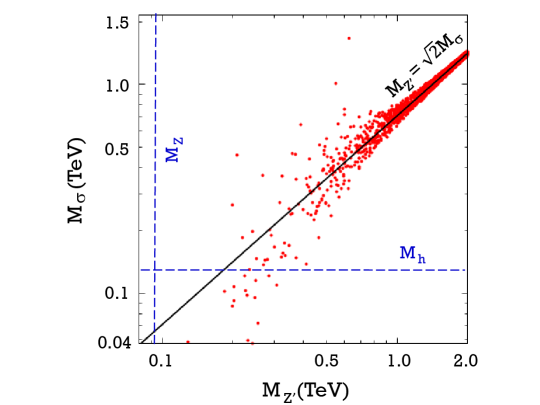
Figure 1: Masses of the Stückelberg scalar $\sigma$ and the extra gauge boson $Z^{\prime}$ when $\zeta^{\prime}$, $\lambda^{\prime}_{1}$ and $\lambda^{\prime}_{2}$ are varied as follows: $0.137\leq\zeta^{\prime}\leq 100$ and $-\sqrt{4\pi}\leq\lambda^{\prime}_{1.2}\leq+\sqrt{4\pi}$. For heavier masses ($M_{Z^{\prime}}>1$ TeV), it may be seen that the ratio $M_{Z^{\prime}}/M_{\sigma}\to\sqrt{2}$. The masses $M_{Z}$ of the $Z$ boson and $M_{h}$ of the Higgs boson are marked on the plot for comparison.

Though we do not make a detailed analysis in this work, it is likely that the lower end of the spectrum, especially the scalar masses lower than 100 GeV, may be ruled out by the existing data. However, there will be plenty of parameter choices which will easily evade these bounds, since the scalar and the $Z^{\prime}$ will simultaneously become heavy. In any case, to make a detailed phenomenological analysis, the Feynman rules for the model require to be worked out in detail. In this model, when we work out the cubic and quartic interactions of the model of Eq. (4.6), it turns out that the interactions of the photon and the $Z$-boson are identical with those of the SM. Thus, one cannot search for signatures of this model by looking for deviations in the usual SM signatures. However, the $Z^{\prime}$ boson and the scalar $\sigma$ will have some new interactions as in the interaction Lagrangian below.

$${\cal L}_{\rm int}=\frac{\mid\!\Phi\!\mid^{2}}{v^{2}}\left[A\left(\partial^{\mu}\sigma\;\partial_{\mu}\sigma-Bv^{2}\sigma^{2}\right)-C\left\{\left(\partial^{\mu}Z^{\prime}_{\mu}\right)^{2}-Dv^{2}Z^{\prime\mu}Z^{\prime}_{\mu}\right\}+v\left(EZ^{\prime}_{\mu}\partial^{\mu}\sigma+F\sigma\partial^{\mu}Z^{\prime}_{\mu}\right)\right]$$

where

$$\mid\!\Phi\!\mid^{2}=\varphi^{+}\varphi^{-}+\frac{1}{2}\left(h^{0}\right)^{2}+\frac{1}{2}\left(\varphi^{0}\right)^{2}+vh^{0}$$ (5.3)

and

$$A = \frac{2\lambda^{\prime}_{1}}{\zeta^{\prime}+\lambda^{\prime}_{1}-\lambda^{\prime}_{2}}$$

$$B = \frac{\lambda^{\prime}_{2}(\zeta^{\prime}-\lambda^{\prime}_{2})}{2\lambda^{\prime}_{1}}$$

$$C = \frac{4\lambda^{\prime}_{2}(\zeta^{\prime}+\lambda^{\prime}_{1}-\lambda^{\prime}_{2})}{\zeta^{\prime}(\zeta^{\prime}-\lambda^{\prime}_{2})}$$

$$D = \frac{\zeta^{\prime 2}\lambda^{\prime}_{1}(\zeta^{\prime}-\lambda^{\prime}_{2})}{2\lambda^{\prime}_{2}(\zeta^{\prime}+\lambda^{\prime}_{1}-\lambda^{\prime}_{2})^{2}}$$

$$E = \frac{2\lambda^{\prime}_{1}\sqrt{\zeta^{\prime}}}{\zeta^{\prime}+\lambda^{\prime}_{1}-\lambda^{\prime}_{2}}$$

$$F = \frac{2\lambda^{\prime}_{2}}{\sqrt{\zeta^{\prime}}}$$ (5.4)

The vertices of these interactions can be read off from this equation, and are listed in Figure 2. As a quick check, we can see that in the decoupling limit, i.e. when $\zeta^{\prime}\to\infty$ (equivalently, when $\lambda^{\prime}_{1,2}\to 0$), the parameters in Eq. (5.4) reduce to

$$A \to \frac{2\lambda^{\prime}_{1}}{\zeta^{\prime}}\qquad\qquad\qquad C\to\frac{4\lambda^{\prime}_{2}}{\zeta^{\prime}}\qquad\qquad\qquad E\to\frac{2\lambda^{\prime}_{1}}{\sqrt{\zeta^{\prime}}}$$

$$B \to \frac{\zeta^{\prime}\lambda^{\prime}_{2}}{2\lambda^{\prime}_{1}}\ \ \qquad\qquad\quad D\to\frac{\zeta^{\prime}\lambda^{\prime}_{1}}{2\lambda^{\prime}_{2}}\qquad\qquad\quad\ \ F\to\frac{2\lambda^{\prime}_{2}}{\sqrt{\zeta^{\prime}}}$$ (5.5)

Figure 2: Feynman vertices for the new bosonic interactions of the $\sigma$ and $Z^{\prime}$ fields.

Thus the only couplings which do not vanish are

$$AB\to\lambda^{\prime}_{2}\qquad\qquad\qquad CD\to 2\lambda^{\prime}_{1}$$ (5.6)

which remain perturbative because the $\lambda^{\prime}_{1,2}$ are perturbative. However, these may get further constrained by the non-observation of the interactions of Figure 2. A related issue is the presence of derivative couplings and hence a strong momentum-dependence of the cubic and quartic couplings, which could, in principle, lead to unitarity violation at a scale significantly higher than the electroweak scale. This does not seem to happen in $U(1)$ Stückelberg models [15]. However, such an analysis for the present model could be interesting in its own right, for, if unitarity is violated, it would mean that the Stückelberg mechanism only works within the framework of an effective theory. However, we defer this analysis to a future work [14].

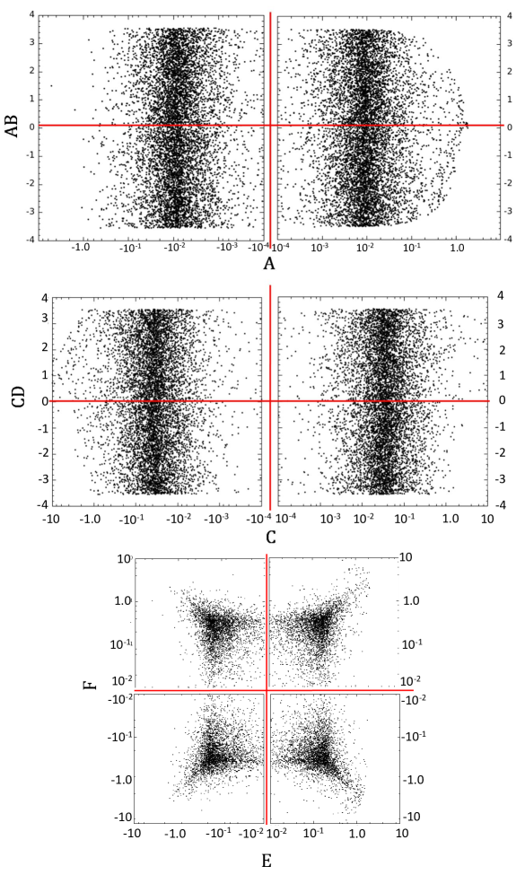
Figure 3: Scatter plots showing the variation of the coupling parameters $A$, $AB$, $C$, $CD$, $E$ and $F$ with random variations in the parameters $\zeta^{\prime}$, $\lambda^{\prime}_{1}$ and $\lambda^{\prime}_{2}$ within their allowed ranges. The coordinate axes are marked in red.

Nevertheless, even apart from the decoupling limit, we can form an idea about the strength of the couplings $A$, $AB$, $C$, $CD$, $E$ and $F$ by varying the independent parameters $\zeta^{\prime}$, $\lambda^{\prime}_{1}$ and $\lambda^{\prime}_{2}$ between their allowed ranges, as we have done above for the masses of the $\sigma$ and the $Z^{\prime}$. The results are shown in Figure 3. It may be seen that the parameters $A$ and $C$ are mostly restricted to the order $10^{-3}$ and $10^{-2}$ respectively, while the product couplings $AB$ and $CD$ vary almost uniformly over the full allowed range. The couplings $E$ and $F$ remain mostly smaller than unity, with a few outlying values. We may conclude, therefore, that even if perturbative unitarity is breached in this model, it will happen at a energy at least an order of magnitude above the electroweak scale, i.e. a few TeV, which is currently unattainable at existing collider machines.

Finally, we come to the gauge-fermion interactions. As usual, these arise from

$${\cal L}_{f}= \sum_{i=k}^{3} \bigl{[}i\bar{L}_{Lk}\gamma^{\mu}{\cal D}_{\mu}^{(L)}L_{Lk}+i\bar{\ell}_{Rk}\gamma^{\mu}D_{\mu}^{(\ell)}\ell_{Rk}$$ (5.7)

$$\!\!\!\!\!+\ i\bar{Q}_{Lk}\gamma^{\mu}{\cal D}_{\mu}^{(Q)}Q_{Lk}+i\bar{u}_{Rk}\gamma^{\mu}D_{\mu}^{(u)}u_{Rk}+i\bar{d}_{Rk}\gamma^{\mu}D_{\mu}^{(d)}d_{Rk}\bigr{]}$$

where the covariant derivatives ${\cal D}_{\mu}$ on the $SU(2)_{L}$ doublets $L_{L}^{T}=(\!\!\begin{array}[]{cc}\nu_{L\ell}&\ell_{L}\end{array}\!\!)$ and $Q_{L}^{T}=(\!\!\begin{array}[]{cc}u_{L}&d_{L}\end{array}\!\!)$ are defined in Eq. (4.33) and the covariant derivative on the singlets $\ell_{R}$, $u_{R}$ and $d_{R}$ are defined as

$$D_{\mu}=\partial_{\mu}-ig\cos\theta_{W}Q_{Z}Z_{\mu}-ig\sin\theta_{W}QA_{\mu}-igQ_{Z}^{\prime}Z^{\prime}_{\mu}$$ (5.8)

where

$$Q_{Z} = -\frac{b\tan\theta_{W}}{2\sqrt{2}}=\frac{1}{2}Y_{\rm SM}\tan^{2}\theta_{W}$$

$$Q = \frac{b}{2\sqrt{2}\tan\theta_{W}}=\frac{1}{2}Y_{\rm SM}$$

$$Q_{Z^{\prime}} = \frac{a}{2\sqrt{2}}=\frac{\eta}{2\sqrt{2}}Y_{\rm SM}$$ (5.9)

In Eq. (5.9), the $Z$ boson and photon interactions are the same as in the SM, as was the case with the Higgs and SM gauge sectors. Thus we will get new interactions only from the $Z^{\prime}$ terms, which can be worked out as

$${\cal L}_{Z^{\prime}f\bar{f}}=\sum_{f}-\frac{g\eta}{4\sqrt{2}}\overline{\psi}_{f}\gamma^{\mu}\left(c^{\prime}_{Vf}+c^{\prime}_{Af}\gamma_{5}\right)\psi_{f}$$ (5.10)

where the generation-independent constants $c^{\prime}_{Vf}$ and $c^{\prime}_{Af}$ are listed in Table 1. This leads to the Feynman vertices in Figure 4.

It must be noted that this pattern of couplings is not unique, but arises only when the simplest ansatz for anomaly cancellation, i.e. $Y\propto Y_{\rm SM}$ is taken. Naturally, this retains the generation-universality observed in the SM and may not be the best choice to explain the flavour anomalies mentioned in the Introduction. However, in that case, one can always pick up one or other of the many different ansätze proposed in $U(1)$-extended SM scenarios [16], and use it in conjunction with the mass generation mechanism proposed in this work.

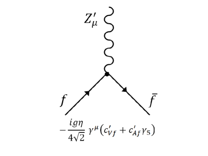
Figure 4: Feynman vertex for the $Z^{\prime}$ coupling with fermions. The constants $c^{\prime}_{Vf}$ and $c^{\prime}_{Af}$ are listed in Table 1.

To get a comparison between the couplings of the $Z^{\prime}$ boson with those of the $Z$ boson, we have plotted the vector and axial vector couplings of both in Figure 5. The quantities plotted for the $Z$ boson are

$$v_{f\bar{f}}(Z)=\frac{g}{4\cos\theta_{W}}c_{Vf}\qquad\qquad a_{f\bar{f}}(Z)=\frac{g}{4\cos\theta_{W}}c_{Af}$$ (5.11)

and for the $Z^{\prime}$ boson are

$$v_{f\bar{f}}(Z^{\prime})=\frac{g\eta}{4\sqrt{2}}c^{\prime}_{Vf}\qquad\qquad a_{f\bar{f}}(Z^{\prime})=\frac{g\eta}{4\sqrt{2}}c^{\prime}_{Af}$$ (5.12)

where, in the four panels, from left to right, $f=\nu,\ell,u$ and $d$ respectively.

$f$	$c^{\prime}_{Vf}$	$c^{\prime}_{Af}$
$\nu_{\ell}$	$Y_{\rm SM}^{(L)}=1$	$-Y_{\rm SM}^{(L)}=-1$
$\ell$	$Y_{\rm SM}^{(L)}+Y_{\rm SM}^{(\ell)}=3$	$-Y_{\rm SM}^{(L)}+Y_{\rm SM}^{(\ell)}=1$
$u$	$Y_{\rm SM}^{(Q)}+Y_{\rm SM}^{(u)}=-\frac{5}{3}$	$-Y_{\rm SM}^{(Q)}+Y_{\rm SM}^{(u)}=-1$
$d$	$Y_{\rm SM}^{(Q)}+Y_{\rm SM}^{(d)}=\frac{1}{3}$	$-Y_{\rm SM}^{(Q)}+Y_{\rm SM}^{(d)}=1$

Table 1: Couplings of the fermions with the $Z^{\prime}$ boson assuming that all the hypercharges are proportional to those in the SM.

A glance at the figure immediately shows that the couplings of the $Z^{\prime}$ boson to fermions can be significantly stronger than those of the $Z$ boson, and hence, in regions which are kinematically favourable, production cross-sections of the $Z^{\prime}$ boson as resonances in fermion pair annihilation can be significantly higher than those of the $Z$ boson. Of course, we also have the decoupling limit $\eta\to 0$ in which the $Z^{\prime}$ has no fermion interactions whatsoever. This, however, is unlikely, since it would call for a fine tuning $Y=g^{\prime}Y_{\rm SM}/\sqrt{2}$ for every fermion hypercharge. We may thus conclude that the $Z^{\prime}$ can have interesting signals at high energy colliders such as the LHC and its upgrades, no less than at a high energy $e^{+}e^{-}$ collider. The study of these will be taken up in a future work [14].

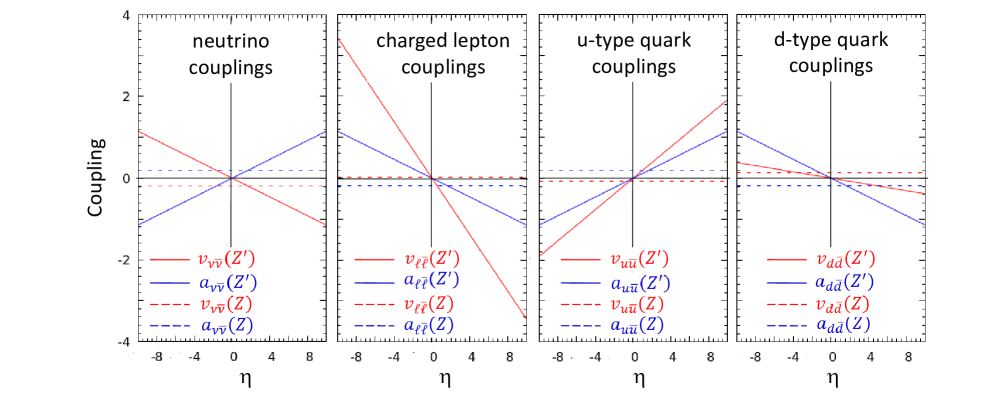
Figure 5: Fermion couplings of the $Z$ and $Z^{\prime}$ bosons, showing their variation with the parameter $\eta$. The range $-10\leq\eta\leq 10$ ensures that all these couplings stay within the perturbative limit.

6 Concluding remarks

In this article, we have reported a careful and detailed development of a $U(1)_{X}$ extended SM, with a Stückelberg mechanism to generate a mass for the extra $Z^{\prime}$ gauge boson instead of a further extension of the Higgs sector. Our analysis differs from previous studies in that we have made the cancellation of (unphysical) bilinear terms in the Lagrangian a keystone of our analysis. As a result, we have obtained constraints which not only provide a gauge-fixing term for the extra gauge boson, but also render the mass matrix extremely simple. This has made it possible to consider, for the first time, new quartic interactions of the Stückelberg scalar, which are permitted by the gauge symmetry. Even with these new interactions, however, the model remains quite minimal and is very economical in new fields and parameters. There are just two new particles, viz., a vector $Z^{\prime}$ and a Stückelberg scalar $\sigma$. Similarly, there are just three parameters in the bosonic part of the theory, which we have chosen to be the $Z^{\prime}$ mass (scaled to the SM vev) and the two new quartic couplings. The advantage of using coupling constants as parameters is, of course, their phenomenological limitation within the perturbative range $-\sqrt{4\pi}<\lambda^{\prime}_{1,2}<+\sqrt{4\pi}$. Thus, the mass scale for new physics is entirely set by the $Z^{\prime}$ mass.

Another nice feature of the model presented here is that the requirement that we obtain the correct charge operator on the Higgs doublet acts as a second constraint, which renders the mass matrix even more simple. As a result, the mixing pattern of gauge bosons becomes such that the interactions of the photon and the $Z$ boson become identical with those in the SM. This immediately renders the model immune from constraints arising from measurement of $Z$ boson interactions, but alas! it also removes a possible phenomenological handle on the new physics. Nevertheless, there do exist a set of interaction vertices between the physical and unphysical fields in the Higgs doublet with the $Z^{\prime}$ and the $\sigma$, which we plan to investigate for possible signals. These new vertices, as we have shown, assume small, but not too small values, which may make these interactions visible at a higher energy and/or luminosity machine.

The fermion sector of the model differs from most other $U(1)_{X}$ extended models in that the couplings of the $Z$ boson remain identical to those in the SM, with no effect of mixing being manifest. The $Z^{\prime}$ boson also couples to fermions, but these couplings depend only on the hypercharge assignments in the model. The requirement that the photon couplings match with QED and the SM, and that the chiral anomalies should cancel put very stringent constraints on the hypercharge choices. This is no different from generic $U(1)_{X}$- extended models, and the same kind of choices are possible. The simplest ansatz, which we have adopted in this article, is to take the hypercharges all proportional to their SM values. This automatically ensures anomaly cancellation, but it drastically reduces the freedom to vary the $Z^{\prime}$ couplings to fermions. While this has the advantage of economy – the parameter space being restricted to that one proportionality factor – it may prove inadequate to explain flavour anomalies as they currently stand. In such a case, perhaps a different ansatz for the fermion-$Z^{\prime}$ couplings may have to be adopted. However, a phenomenological analysis would be needed before we come to any such conclusion.

To make a long story short, then, we have re-examined the possibility that a msssive vector boson $Z^{\prime}$ in a $U(1)$-extended SM can get its mass through a Stückelberg mechanism rather than by invoking a further complication of the symmetry-breaking mechanism of the SM. The answer to this question seems to be in the affirmative. The resultant model, which has several features not considered earlier in the existing literature, cannot be falsified by current data, but it can predict interesting novel signatures at future colliders. It also has the potential to explain flavour physics anomalies. A joint study of such anomalies and possible collider signals in the context of this model will be required in order to make a more definitive statement, and is in the pipeline.

 Acknowledgments: RV is grateful to A. Misra for discussions and acknowledges the DST-INSPIRE for financial support. SR acknowledges extensive discussions with A. Venkata (CEBS, Mumbai) which helped initiate this study. SR acknowledges support of the Department of Atomic Energy, Government of India, under Project Identification No. RTI 4002.

Appendix

In this Appendix, we present the proof that the choice # 1 in Section 4, which is described in Eq. (4.26), does not lead to a physically viable solution. For this choice, we note that $a_{\Phi}$ and $b_{\Phi}$ are arbitrary, and hence $\mu^{2}$ is fixed by Eq. (4.26) as

$$\mu^{2}=\frac{1}{2\cos^{2}\theta_{W}}\left(1+\frac{a_{\Phi}^{2}}{b_{\Phi}^{2}-\tan^{2}\theta_{W}}\right)$$ (A.1)

and the mass matrix is given by Eq. (4.21) as

$$\mathbb{M}=\frac{M_{W}^{2}}{4}\left(\begin{array}[]{ccc}2&-\sqrt{2}a_{\Phi}&-\sqrt{2}b_{\Phi}\\ -\sqrt{2}a_{\Phi}&a_{\Phi}^{2}+4\mu^{2}&a_{\Phi}b_{\Phi}\\ -\sqrt{2}b_{\Phi}&a_{\Phi}b_{\Phi}&b_{\Phi}^{2}\end{array}\right)$$ (A.2)

which has eigenvalues $M_{Z}^{2}=M_{W}^{2}/\cos^{2}\theta_{W}$, $M_{\gamma}^{2}=0$ and

$$M_{Z^{\prime}}^{2}=\frac{M_{W}^{2}}{4}\left(2+a_{\Phi}^{2}+b_{\Phi}^{2}+4\mu^{2}+\sqrt{(2+a_{\Phi}^{2}+b_{\Phi}^{2}-4\mu^{2})^{2}+16\mu^{2}a_{\Phi}^{2}}\right)$$ (A.3)

We can now work out the eigenvectors and obtain the diagonalising matrix $\mathbb{S}$ in terms of which we can write

$$\left(\!\!\begin{array}[]{c}Z_{\mu}\\ A_{\mu}\\ Z^{\prime}_{\mu}\end{array}\!\!\right)=\mathbb{S}\left(\!\!\begin{array}[]{c}W_{\mu}^{3}\\ \widetilde{B}_{\mu}\\ \widetilde{C}_{\mu}\end{array}\!\!\right)$$ (A.4)

The only relevant elements of $\mathbb{S}$ are

$$S_{12}=S_{32}=\frac{b_{\Phi}}{\sqrt{2+b_{\Phi}^{2}}}\qquad\qquad S_{22}=0$$ (A.5)

and these can be obtained simply from the eigenvector corresponding to the vanishing eigenvalue. The covariant derivative of Eq. (4.33) can then be written out in full, but these three elements are the only ones needed to obtain the electric charge operator

$$ie{\cal Q}=\frac{igb_{\Phi}}{\sqrt{2+b_{\Phi}^{2}}}\left(\mathbb{T}_{3}+\frac{b}{b_{\Phi}}\mathbb{I}\right)$$ (A.6)

To obtain the correct value of $e$ we will have to identify

$$\frac{b_{\Phi}}{\sqrt{2+b_{\Phi}^{2}}}=\sin\theta_{W}$$ (A.7)

which immediately leads to $b_{\Phi}^{2}=2\tan^{2}\theta_{W}$ contradicting Eq. (4.26), our starting point. This completes the proof that there is no way we can get the correct electric charge quantum $e$ if we choose the option # 1 in Section 4.