Using newest VLT-KMOS HII Galaxies and other cosmic tracers to test the $\Lambda$CDM tension

Abstract

We place novel constraints on the cosmokinetic parameters by using a joint analysis of the newest VLT-KMOS HII galaxies (HIIG) with the Supernovae Type Ia (SNIa) Pantheon sample. We combine the latter data sets in order to reconstruct, in a model independent way, the Hubble diagram to as high redshifts as possible. Using a Gaussian process we derive the basic cosmokinetic parameters and compare them with those of $\Lambda$CDM. In the case of SNIa we find that the extracted values of the cosmokinetic parameters are in agreement with the predictions of $\Lambda$CDM model. Combining SNIa with high redshift tracers of the Hubble relation, namely HIIG data we obtain consistent results with those based on $\Lambda$CDM as far as the present values of the cosmokinetic parameters are concerned, but find significant deviations in the evolution of the cosmokinetic parameters with respect to the expectations of the concordance $\Lambda$CDM model.

I Introduction

The discovery of the accelerated expansion of the Universe from Supernovae type Ia (SNIa) data [1, 2] has opened a new window for research in Cosmology. Indeed, the analysis of various cosmological probes, including those of Cosmic Microwave Background (CMB) [3, 4, 5], Baryon Acoustic Oscillation (BAO) [6, 7, 8, 9, 10, 11, 12], and cosmic chronometers [13] have provided the general framework of cosmic expansion, namely the universe is in the phase of acceleration at late times. Despite the latter confirmation, the nature of cosmic acceleration remains a mystery, hence a lot of effort has been put in by cosmologists over the last two decades in order to provide a viable explanation concerning the underlying mechanism which is responsible for this phenomenon.

Within the framework of homogeneous and isotropic Universe, the corresponding accelerated expansion can be described by considering either a new form of matter with negative pressure [14, 15, 16, 17, 18, 19, 20] or a modification of gravity [$f(R)$, $f(T)$ theories etc, 21, 22, 23, 24, 25]. Among the large family of cosmological models the present accelerating phase of the universe is quite well described in the context of general relativity together with a cosmological constant – the so called $\Lambda$CDM model. This model is spatially flat, with cold dark matter (CDM) and baryonic matter coexisting with the cosmological constant. However, the $\Lambda$CDM model suffers from well known theoretical problems, namely the coincidence problem and the expected value of the vacuum energy density [26, 27, 28, 29].

Although the $\Lambda$CDM model is consistent with the majority of cosmological data [5], the model seems to currently be in tension with some recent measurements [30, 31, 32, 33, 34], associated with the Hubble constant $H_{0}$ and the present value of the mass variance at 8$h^{-1}$Mpc, namely $\sigma_{8}$. Also [35] performing a combined analysis of SNIa, quasars, and gamma-ray bursts (GRBs), found a $\sim 4\sigma$ tension between the best fit cosmographic parameters with respect to those of $\Lambda$CDM (see also [36]). Recently, [37] continued this study by using the same notations but a relatively larger sample of quasars. They have shown a strong deviation from $\Lambda$CDM at high redshifts. As expected, in light of the aforementioned results, an intense debate is taking place in the literature and our work attempts to contribute to this debate.

In our work, for the first time, we use our new set of high spectral resolution observations of high-z HIIG, obtained with VLT-KMOS [38] along with available HIIG data [39, 40] and combine them with the Type Ia Supernovae (SNIa) data from the Pantheon sample [41] in order to reconstruct the Hubble diagram and thus to place constraints on the main cosmokinetic parameters (deceleration and jerk), as well as to check for deviations from the predictions of the $\Lambda$CDM model. Specifically, in this paper we focus on a model-independent parameterization of the Hubble diagram using the Gaussian process, and investigate its performance against the latest SNIa+HIIG Hubble diagram data. It is crucial to note that we need to introduce a kernel function with a set of hyper-parameters which can be optimized in order to fit the data. The reader may find more details of model-independent methods in [42, 43, 44, 45, 46].

The structure of the current article is as follows. In section II, we briefly review the basic cosmological background equations and present the observational data used. In section III, we present the main properties of the Gaussian process together with the corresponding kernel functions, while in section IV we discuss our results. Finally, we draw our conclusions in section V.

II Background cosmology and data set

Considering a spatially flat FRW cosmology and assuming that the fluid components do not interact with each other, the evolution of the Hubble parameter is given by

$$H^{2}(z)=H_{0}^{2}\left[\Omega_{m0}(1+z)^{3}+\Omega_{r0}(1+z)^{4}+\Omega_{x}(z)\right],$$ (1)

where $H_{0}$ is the Hubble constant, $\Omega_{m0}$ and $\Omega_{r0}$ are the density parameters of matter and radiation at the present time. The parameter $\Omega_{x}(z)$ can be seen as a general function that describes the dark energy component. There are a lot of options for the dark energy component (see the introduction for some references), but the simplest case is a constant density parameter: $\Omega_{\Lambda}(z)=\Omega_{\Lambda 0}=1-\Omega_{m0}-\Omega_{r0}$, namely the well known $\Lambda$CDM model, where the Hubble parameter is written as

$$H^{2}(z)=H_{0}^{2}\left[\Omega_{m0}(1+z)^{3}+\Omega_{r0}(1+z)^{4}+1-\Omega_{m0}-\Omega_{r0}\right].$$ (2)

Of course, it is straightforward to compute the luminosity distance,

$$D_{L}(z)=(1+z)D(z),$$ (3)

where

$$D(z)=\int_{0}^{z}\frac{dx}{H(x)},$$ (4)

is the comoving distance, while the luminosity distance usually is related with the distance modulus,

$$\mu(z)=5\log_{10}D_{L}(z)+25.$$ (5)

where the distance $D_{L}$ is given in Mpc. Having a sample of standard candles in the universe and measuring their distance moduli, it is straightforward to compute the Hubble parameter from

$$H(z)=\left[D^{\prime}(z)\right]^{-1},$$ (6)

where prime denotes derivative with respect to redshift and $D^{\prime}(z)\neq 0$. Therefore, given the luminosity distance data, one can reconstruct the comoving distance and then find the corresponding Hubble parameter. The step that follows is to derive the cosmokinetic parameters, namely

$$q(z) =(1+z)\frac{H^{\prime}(z)}{H(z)}-1,$$ (7)

$$j(z) =(1+z)^{2}\left[\frac{H^{\prime\prime}(z)}{H(z)}+(\frac{H^{\prime}(z)}{H(z)})^{2}\right]-2(1+z)\frac{H^{\prime}(z)}{H(z)}+1,$$ (8)

where $q(z)$ and $j(z)$ are the deceleration and jerk parameters, respectively. These parameters provide a useful parametrization, in these kind of studies, to test the performance of a given cosmological model against the observational data.

Below we briefly present the type of observational data used in reconstructing the Hubble diagram.

• HIIG data: In a large sequence of articles, [38, 39, 47, 48, 40, 49, 50, 51, 52] HIIGs have been proposed as alternative tracers of the cosmic expansion extending the Hubble diagram on epochs beyond the range of available SNIa data. We use the HIIG sample as provided by [38] (for a full description of the data see [38]). This data set includes 181 entries, which can be split in the local sample (107 objects: $z\leq 0.16$) and a high redshift sample which contains 29 KMOS, 15 MOSFIRE, 6 XShooter and 24 literature objects [38]. The redshift span of the HIIG data is: $0.088\leq z\leq 2.5$.

• SNIa data: In our analysis we utilize the data of the Pantheon SNIa sample (considering only statistical uncertainties) [41], which combines the SNIa sources of the PanSTARRS1 (PS1) Medium Deep Survey with a large number of other surveys, to compare the two distinct and independent tracers of the Hubble relation.

Before reconstructing the Hubble parameter, we perform a Bayesian inference considering the $\Lambda$CDM model to find the cosmokinetic parameters at the present time. In Figure (1), we present the observational data and on top we plot the predictions of $\Lambda$CDM model by using the best fit values, namely $\Omega_{m0}=0.282\pm 0.012$ and $H_{0}=71.86\pm 0.22$. The comparison indicates that there is a small difference between data and model at high redshifts. Additionally, in Figure (2) we present the contour plot in $H_{0}-\Omega_{m0}$ plane. Notice that we do not consider the radiation term in Eq.(1) since we are well inside the matter/dark energy dominated eras.

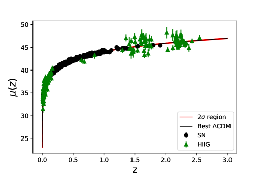
Figure 1: The distance moduli as a function of redshift of the SNIa and HIIG are shown as points with uncertainties. The continuous curve is the best-fit $\Lambda$CDM Hubble function.

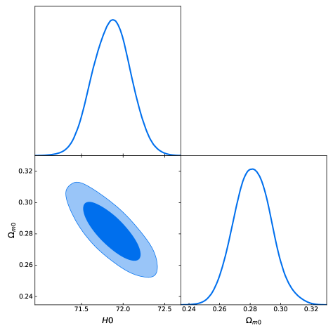
Figure 2: 1 and 2 $\sigma$ confidence levels in the $H_{0}-\Omega_{m0}$ plane and their posterior distributions for the $\Lambda$CDM model.

III Gaussian process as a model independent method

In general, based on the luminosity distance, there are two main avenues in order to study the Hubble diagram, aiming to understand the expansion rate of the universe. The first choice is to impose a cosmological model and through standard lines to extract the corresponding form of the luminosity distance. Subsequently, the model is fitted to the data in order to put constraints on the corresponding free parameters. Obviously, this approach is a model-dependent method, since different models provide different functional forms for the luminosity distance. The second choice is to use a model independent method in building the Hubble diagram via the observational data [42, 43, 44, 45], hence we do not need to impose a particular model as an underlying cosmology. In this context, one of the model independent methods which is widely used in this kind of studies is the Gaussian process (GP), and indeed in the present article we attempt to test the performance of GP against the available Hubble diagram data.

Now let us briefly present the basic steps of the method. The GP is a sequence of Gaussian random variables (RV), which can be modeled with a multivariate Gaussian distribution.

Generally, for a given data set $M$

$$M=\{(x_{i},y_{i})|i=1,..,n\},$$ (9)

our target is to build a function which can reproduce the data in a model independent way, assuming that the data points can be modeled with a GP, $y\sim GP(\mu(x),K(x_{i},x_{j}))$, where $\mu(x)$ provides the mean value at each point and $K$ is the so called GP kernel which indicates the covariance function between different points. In this case, the diagonal (off-diagonal) terms of the kernel give the uncertainty at each point (correlation between different points). Now, in order to build a continuous function we need to compute the prediction of GP at a set of arbitrary points ($x^{\star}$) rather than at the observational points ($x$). In this context, it is an easy task to compute the mean and the covariance function at these new points according to [54]:

$$\mu^{\star} = K(x,x^{\star})[K(x,x^{\star})+C_{D}]^{-1}Y$$ (10)

$$\Sigma^{\star} = K(x^{\star},x^{\star})-K(x^{\star},x)[K(x,x^{\star})+C_{D}]^{-1}K(x,x^{\star}),$$ (11)

where $C_{D}$ is the covariance matrix of the data, $Y$ is the column vector of observation $y_{i}$, while a zero mean prior has been considered in deriving the above equations. Having obtained these quantities, one can generate many functions at $(x^{\star})$ using the expression

$$f(x^{\star})\sim N(\mu^{\star},\Sigma^{\star}),$$

where $N(\mu^{\star},\Sigma^{\star})$ is a multivariate Gaussian distribution.

Regarding the kernel function, there are a variety of options depending of course on the characteristics of the data. The best known kernel is the squared exponential kernel

$$K(x_{i},x_{j})=\sigma_{f}^{2}\exp{\left(-\frac{(x_{i}-x_{j})^{2}}{2l^{2}}\right)},$$ (12)

where $\sigma_{f}^{2}$ and $l$ are two hyper-parameters of the kernel. Since the results might depend on the selected kernel, it is common procedure to consider several kernels. In our analysis, we utilize the Matren $\nu=7/2$ and $\nu=9/2$ kernels along with equation (12) as detailed in [46].

It is interesting to mention that the GP method provides the reconstructed function $f(x)$ as well as the corresponding derivatives. Indeed, since the derivative of a GP function is another GP, the corresponding derivative with respect to variable $x$ is given by

$$f^{\prime}(x)\sim GP\left(\mu^{\prime}(x),\frac{\partial^{2}K}{\partial x_{i}\partial{x_{j}}}\right)$$

Concerning the second and third derivatives we refer the reader for more details to [55, 56].

To conclude this section let us summarize the steps that we need to follow in order to reconstruct the Hubble diagram and the corresponding cosmokinetic parameters.

1. We convert the distance modulus to luminosity distance and finally to comoving distance,
   

2. we obtain the GP of $D(z)$ using different kernels and different data sets, by employing the scikit-learn library [57],
   

3. for $D^{\prime}(z)=0$, we see from equation (6) that $H(z)$ goes to infinity, hence we exclude these solutions (if any) from the reconstruction process,
   

4. and finally, we generate many reconstructed comoving distances as well as its first and second derivatives, and then compute the cosmokinetic parameters [e.g $H(z)$,$q(z)$ and $j(z)$].

IV The estimated cosmokinetic parameters

In this section we discuss the main results of our analysis, utilizing the aforementioned data sets and methods. In order to reconstruct $H(z)$, $q(z)$ and $j(z)$, we use the $D(z)$, $D^{\prime}(z)$ and $D^{\prime\prime}(z)$ functions described in section II. In Figures 4 and 5 we present our results considering the Gaussian kernel. We have verified that considering other kernels the results remain unaltered. Having obtained the reconstructed cosmokinetic parameters we compute the corresponding uncertainties at each redshift. Since the values of the reconstructed cosmokinetic parameters follow a normal distribution at each redshift, their uncertainties are given by the standard deviation at those points. To check the robustness of the results, we sample $D(z)$, $D^{\prime}(z)$ and $D^{\prime\prime}(z)$ several times and compute the cosmokinetic parameters from different samples and verified that the results are stable.

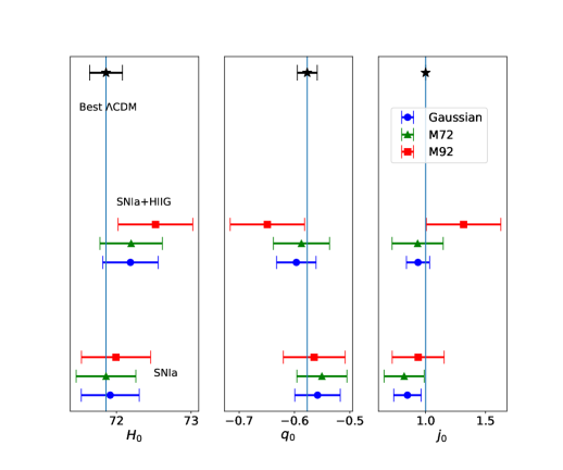
Figure 3: Cosmokinetic parameters at the present time considering different kernels and data sets. Blue circles, green triangles and red squares show the results for Gaussian, Matren $(\nu=3.5)$ and Matren $(\nu=4.5)$, respectively. The best fit $\Lambda$CDM value, considering all the data, is shown by a black star at the top of each panel.

In Table (1), we provide a summary of the obtained results. We also show the extracted cosmokinetics parameters in Figure (3) at the present time.

	Gaussian	Matren $\nu=7/2$	Matren $\nu=9/2$
SNIa	$H_{0}$= $71.92\pm 0.38$ $q_{0}$=$-0.558\pm 0.040$ $j_{0}$=$0.840\pm 0.110$	$H_{0}$=$71.86\pm 0.40$ $q_{0}$=$-0.550\pm 0.045$ $j_{0}$=$0.820\pm 0.170$	$H_{0}$=$71.99\pm 0.46$ $q_{0}$=$-0.564\pm 0.050$ $j_{0}$=$0.940\pm 0.220$
SNIa+HIIG	$H_{0}$=$72.18\pm 0.37$ $q_{0}$=$-0.596\pm 0.035$ $j_{0}$=$0.936\pm 0.096$	$H_{0}$=$72.19\pm 0.42$ $q_{0}$=$-0.587\pm 0.050$ $j_{0}$=$0.933\pm 0.213$	$H_{0}$=$72.52\pm 0.50$ $q_{0}$=$-0.648\pm 0.067$ $j_{0}$=$1.310\pm 0.310$

Table 1: Cosmokinetic parameters at the present time for different data sets and kernels.

Overall, we find that our results are in very good agreement with those of [46] who used Gamma ray bursts instead of HIIG and a similar approach to the one presented here. The current GP analysis shows that close to the present time we acquire $\sim 1\sigma$ compatibility in all cases. Specifically, the dimensionless parameters $q_{0}$ and $j_{0}$ are constrained to an interval which includes the concordance $\Lambda$CDM model and there is only a small deviation in $H_{0}$ considering all data sets.

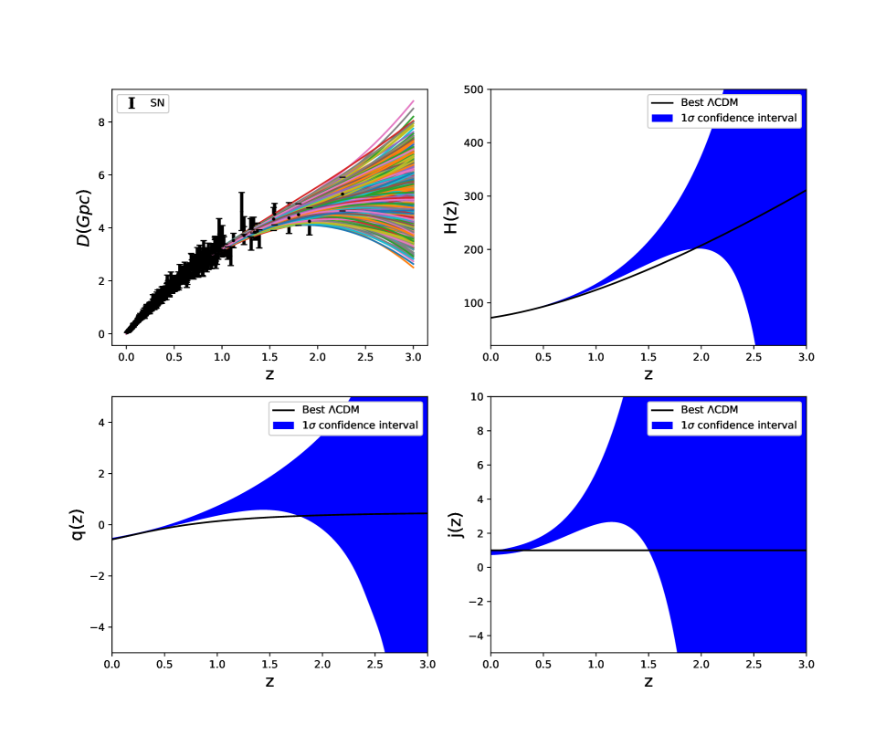
Figure 4: The reconstruction of the cosmokinetic parameters using SNIa data with Gaussian kernel.

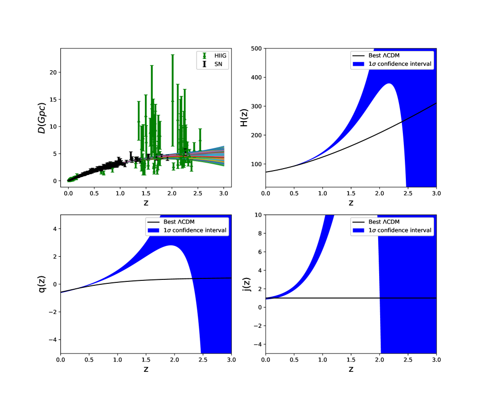
Figure 5: The reconstruction of cosmokinetic parameters using SNIa and HII data with Gaussian kernel.

	Redshifts	H(z)	q(z)	j(z)
SNIa	$z=0.5$ $z=1$ $z=1.5$	$1.5$   $2.0$   $1.5$	$1.6$ $2.1$ $1.5$	$2.1$ $2.0$ $1.0$
SNIa+HIIG	$z=0.5$ $z=1$ $z=1.5$	$1.6$ $4.8$ $4.0$	$3.2$ $5.8$ $4.1$	$5.0$ $4.9$ $2.5$

Table 2: Amount of $\sigma$ deviation ($\Delta X(z)$) from the best $\Lambda$CDM model at 3 different redshifts.

Next we focus on the evolution of the cosmokinetic parameters. For the given cosmological quantity $X(z)$, namely $H(z)$, $q(z)$, and $j(z)$ we estimate the corresponding deviation $\Delta X$, with respect to the $\Lambda$CDM solution

$$\Delta X(z)=\left[\frac{X(z)-X_{\Lambda}(z)}{\sigma_{X}(z)}\right],$$ (13)

where $\sigma_{X}(z)$ is the uncertainty of the reconstructed $X$ parameter at redshift $z$. In Table (2) we provide an overall presentation of the relative deviation for three different cosmic epochs, namely $z=0.5,1$ and 1.5. Also, in Figures 4 and 5 we show the evolution of the reconstructed cosmokinetic parameters. At this point we need to mention that for $z>1.5$ the deviation starts to decay due to large uncertainties in the reconstruction of the Hubble relation and its derivatives, hence we restrict our analysis to the aforementioned cosmic epochs.

In the case of SNIa data, the deviation of the reconstructed cosmokinetic parameters with respect to those of the $\Lambda$CDM lies in the interval $[1\sigma,2.1\sigma]$, implying that these data alone do not indicate any significant difference. These results remain robust regardless of the form of the corresponding kernel used during the reconstruction process. First, including HIIG data, the deviation in all $H(z)$, $q(z)$ and $j(z)$ is significant for $z\sim 1$ (or $1.5$). Specifically, close to $z=1$ (or $z=1.5$), we find that the reconstructed Hubble parameter deviates from the best $H_{\Lambda}(z)$ by $\sim 4.8\sigma,(\sim 4\sigma)$. Moreover for the total data set, SNIa+HIIG, we see that prior to the present epoch, since SNIa data dominate the Hubble relation, the reconstructed Hubble parameter tends to that of $\Lambda$CDM, namely the relative deviation is quite small $\sim 1.6\sigma$. Regarding the deceleration parameter, we observe a clear deviation from the $\Lambda$CDM model, which can reach up to $\sim 5.8\sigma$ (or $4.1\sigma$) at $z=1$ (or $z=1.5$) [see SNIa+HIIG in Table(2)]. Concerning the jerk parameter, there is a visible deviation from the $\Lambda$CDM model, where the maximum tension is $\sim 5\sigma$ at $z=0.5$ for the set SNIa+HIIG.

Finally, we run our code only for HIIG data and in Figure (6) we show the corresponding results. We find that the performance of the reconstruction method is rather poor with respect to that for SNIa, but this is not surprising because in our case we have only 181 HIIG, most of them at $z<0.16$ (106 objects) a region of space where differences between cosmological models are almost negligible. However, the strength of our results is that the HIIG sample includes 69 objects with $z>1.4$ vs. only 6 SNIa. Indeed from Figure (6) we observe that despite the poor reconstruction of the cosmic expansion it is encouraging that the jerk parameter starts to deviate from unity at relatively high-z. This is an indication for deviations in the evolution of $j(z)$ with respect to the expectations of the usual $\Lambda$CDM model. Of course as we have already discussed above combining HIIG with SNIa we obtain similar results to those of [37, 46], where they have combined SNIa with other potential high-z cosmic tracers (quasars, GRBs) in order to extend the Hubble relation to as high redshifts as possible.

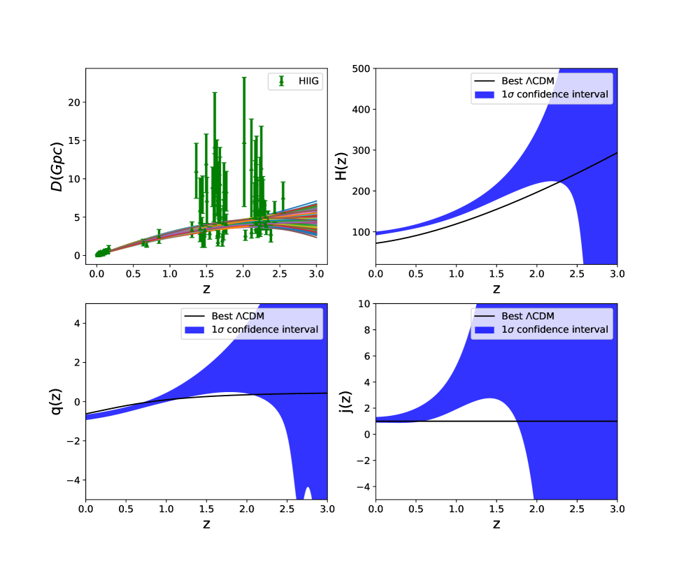
Figure 6: The reconstruction of cosmokinetic parameters using only HIIG data with Gaussian kernel.

V Discussion and Conclusions

Although the concordance $\Lambda$CDM model is considered to be in agreement with the majority of observational data, lately there have been heated debates in the literature since it seems to be in tension with some recent measurements, related to the Hubble constant $H_{0}$ and the current value of the mass variance in spheres of 8 $h^{-1}$ Mpc radius [31, 30, 33, 32, 34].

From the view point of the Hubble diagram, [35, 37] combining the nominal standard candles (SNIa) with other probes such as quasars and Gamma-Ray Bursts obtained a $\sim 4\sigma$ tension between the best fit cosmokinetic parameters and the $\Lambda$CDM expectations (see also Lusso et al. [37], Mehrabi and Basilakos [46]). Whether these tensions are the result of yet unknown systematic errors or hint towards new Physics is still unclear. Therefore, within the framework of the traditional $\Lambda$CDM model, testing the validity of the Hubble diagram at large redshifts is considered one of the most crucial tasks in cosmology, hence it is important to minimize the amount of assumptions needed to successfully complete such an effort. One possible avenue is to reconstruct the Hubble diagram in a model independent way, and thence to estimate the cosmokinetic parameters.

In this article we worked along the above lines and in particular we used HIIG as alternative tracers of the Hubble expansion and combined them with the SNIa data aiming to reconstruct the Hubble diagram in a model independent way and thus to constrain the corresponding cosmokinetic parameters. We performed a reconstruction method which is based on the so called GP method [55, 56, 46] in the context of three different kernels. In the case of SNIa data we found that the cosmokinetic parameters, extracted from the Gaussian process, are consistent with those of $\Lambda$CDM at the present time. Including HIIG in the analysis, we didn’t find significant deviations from $\Lambda$CDM, as far as the current value of cosmokinetic parameters is concerned.

Then we focused on the evolution of the cosmokinetic parameters and we verified that it is not significantly affected by the choice of the kernel. Since our method has some limitations due to large uncertainties in reconstructing properly the Hubble relation at large enough redshits, we have restricted our analysis to intermediate cosmic epochs, namely $z\in[1,1.5]$. For this redshift interval we found that the estimated cosmokinetic parameters significantly deviate from those of the usual $\Lambda$CDM model. Indeed for the SNIa+HIIG combination, the corresponding deviation, close to $z=1.5$, can reach up to $\sim 4\sigma$ in the case of $H(z)$, $\sim 4.1\sigma$ in the case of $q(z)$ and $\sim 2.5\sigma$ for $j(z)$, while for $z=1$ the corresponding deviations become even larger.

In a nutshell, we argue that the potential benefit of having standard tracers for cosmology at high redshifts makes it tempting to try and use HIIG to constrain the cosmological expansion history in a way similar to SNIa. Notice that our team has thoroughly studied in a series of papers (see [50, 40]) the question of which is the most efficient strategy to tighten the cosmological constraints provided by fitting the Hubble relation. Using extensive Monte-Carlo simulations we have found that by using a number of $\sim 300$ high z tracers, even with a relatively large distance modulus uncertainty, we can reduce significantly the cosmological parameter solution space. Currently, our group is designing the appropriate KMOS-VLT observations of high-z objects aiming to include $\sim$100 additional entries in the HIIG sample which are expected to substantially improve the performance of our method in reconstructing (in a model-independent way) the Hubble relation, hence to use cosmokinetics in order to test the validity of the concordance $\Lambda$CDM.

The use of HIIG as distance indicators and to deduce cosmological parameters ($\Omega_{m0}$, $H_{0}$, equation of state parameter etc) is not new. Since the work, e.g., of [58], our group has refined the method and, following e.g. [50, 40, 48] simulations, have embarked in a concerted observational programme destined to improve the pool of data, in particular at higher z ranges, where differences between cosmological models are more prominent, and on better understanding the systematic errors in the method. Specifically, [59] have used the data to investigate performance of some well-known models including the $\Lambda$CDM, wCDM (quintessence) and $R_{h}=ct$ universe. Their analysis indicated that the $R_{h}=ct$ model is strongly favored over wCDM. On the other hand, [60] have used a sub-sample of our HIIG data and the GP method in order to reconstruct the Hubble relation, without estimating the cosmokinetic parameters. In addition, in a more recent work [61], have combined two compilations of HIIG data with quasars, BAOs, cosmic expansion $H(z)$ data and SNIa data in order to place constrains on several cosmological models.

Overall, we argue that by including high-$z$ alternative tracers in the Hubble diagram, there is a discrepancy/tension between the measured cosmokinetic parameters with those of the concordance $\Lambda$CDM model in intermediate cosmic epochs, possibly an indication for new Physics, if one would eventually exclude systematics and small-number statistics.

Therefore, in order to clarify the situation it is necessary to increase our HIIG sample, especially at high redshifts. Indeed this has been shown to be crucial, since according to [50, 48], a possible deviation from $\Lambda$CDM could in principle be detected when using a few hundreds of high redshift HIIG in the $1.5\leq z\leq 4$ interval.

In the current work we used the newest HIIG sample that contains in total 181 entries, out of which 74 are high redshift HIIG, already providing very promising results. In the future our group is designing the appropriate KMOS-VLT observations of high-z objects aiming to add $\sim$ 100 additional HIIG in the sample which are expected to substantially improve the performance of our method in reconstructing (in a model-independent way) the Hubble relation, and thus the validity of the concordance $\Lambda$CDM model will be effectively tested via the cosmokinetic analysis.

References

- Riess et al. [1998] A. G. Riess, A. V. Filippenko, P. Challis, and et al., AJ 116, 1009 (1998).
- Perlmutter et al. [1999] S. Perlmutter, G. Aldering, G. Goldhaber, and et al., ApJ 517, 565 (1999).
- Komatsu et al. [2011] E. Komatsu, K. M. Smith, J. Dunkley, and et al., ApJS 192, 18 (2011).
- Planck Collaboration XIV [2016] Planck Collaboration XIV (Planck Collaboration), Astron.Astrophys. 594, A14 (2016).
- Aghanim et al. [2018] N. Aghanim et al. (Planck), (2018), arXiv:1807.06209 [astro-ph.CO] .
- Eisenstein et al. [2005] D. J. Eisenstein et al. (SDSS Collaboration), ApJ 633, 560 (2005).
- Percival et al. [2010] W. J. Percival, B. A. Reid, D. J. Eisenstein, and et al., MNRAS 401, 2148 (2010).
- Blake et al. [2011] C. Blake et al., Mon. Not. Roy. Astron. Soc. 415, 2876 (2011), arXiv:1104.2948 [astro-ph.CO] .
- Reid et al. [2012] B. A. Reid, L. Samushia, M. White, W. J. Percival, M. Manera, et al., MNRAS 426, 2719 (2012).
- Abbott et al. [2019] T. M. C. Abbott et al. (DES), Mon. Not. Roy. Astron. Soc. 483, 4866 (2019), arXiv:1712.06209 [astro-ph.CO] .
- Alam et al. [2017] S. Alam et al. (BOSS), Mon. Not. Roy. Astron. Soc. 470, 2617 (2017), arXiv:1607.03155 [astro-ph.CO] .
- Gil-Marín et al. [2018] H. Gil-Marín et al., Mon. Not. Roy. Astron. Soc. 477, 1604 (2018), arXiv:1801.02689 [astro-ph.CO] .
- Farooq et al. [2017] O. Farooq, F. R. Madiyar, S. Crandall, and B. Ratra, Astrophys. J. 835, 26 (2017), arXiv:1607.03537 [astro-ph.CO] .
- Weinberg [1989] S. Weinberg, Reviews of Modern Physics 61, 1 (1989).
- Peebles and Ratra [2003] P. Peebles and B. Ratra, Rev. Mod. Phys. 75, 559 (2003).
- Copeland et al. [2006] E. J. Copeland, M. Sami, and S. Tsujikawa, IJMP D15, 1753 (2006).
- Chiba et al. [2009] T. Chiba, S. Dutta, and R. J. Scherrer, Phys. Rev. D 80, 043517 (2009).
- Amendola and Tsujikawa [2010] L. Amendola and S. Tsujikawa, Dark Energy: Theory and Observations (Cambridge University Press, Cambridge UK, 2010).
- Mehrabi [2018] A. Mehrabi, Phys. Rev. D97, 083522 (2018), arXiv:1804.09886 [astro-ph.CO] .
- Mehrabi and Basilakos [2018] A. Mehrabi and S. Basilakos, Eur. Phys. J. C78, 889 (2018), arXiv:1804.10794 [astro-ph.CO] .
- Schmidt [1990] H.-J. Schmidt, Astron. Nachr. 311, 165 (1990).
- Magnano and Sokolowski [1994] G. Magnano and L. M. Sokolowski, Phys. Rev. D 50, 5039 (1994).
- Dobado and Maroto [1995] A. Dobado and A. L. Maroto, Phys. Rev. D 52, 1895 (1995).
- Capozziello et al. [2003] S. Capozziello, S. Carloni, and A. Troisi, Recent Res. Dev. Astron. Astrophys. 1, 625 (2003).
- Carroll et al. [2004] S. M. Carroll, V. Duvvuri, M. Trodden, and M. S. Turner, Phys. Rev. D 70, 043528 (2004).
- Weinberg [1989] S. Weinberg, Reviews of Modern Physics 61, 1 (1989).
- Padmanabhan [2003] T. Padmanabhan, Phys. Rep. 380, 235 (2003), arXiv:hep-th/0212290 [hep-th] .
- Perivolaropoulos [2008] L. Perivolaropoulos, “Six puzzles for lcdm cosmology,” (2008), arXiv:0811.4684 [astro-ph] .
- Padilla [2015] A. Padilla, “Lectures on the cosmological constant problem,” (2015), arXiv:1502.05296 [hep-th] .
- Verde et al. [2019] L. Verde, T. Treu, and A. G. Riess, Nature Astronomy 3, 891–895 (2019).
- Solà et al. [2017] J. Solà, A. Gómez-Valent, and J. de Cruz Pérez, Phys. Lett. B774, 317 (2017), arXiv:1705.06723 [astro-ph.CO] .
- di Valentino et al. [2021a] E. di Valentino et al., Astroparticle Physics 131, 102605 (2021a).
- di Valentino et al. [2021b] E. di Valentino et al., Astroparticle Physics 131, 102604 (2021b).
- Perivolaropoulos and Skara [2021] L. Perivolaropoulos and F. Skara, (2021), arXiv:2105.05208 [astro-ph.CO] .
- Lusso et al. [2019] E. Lusso, E. Piedipalumbo, G. Risaliti, M. Paolillo, S. Bisogni, E. Nardini, and L. Amati, Astron. Astrophys. 628, L4 (2019), arXiv:1907.07692 [astro-ph.CO] .
- Risaliti and Lusso [2019] G. Risaliti and E. Lusso, Nat. Astron. 3, 272 (2019), arXiv:1811.02590 [astro-ph.CO] .
- Lusso et al. [2020] E. Lusso, G. Risaliti, E. Nardini, G. Bargiacchi, M. Benetti, S. Bisogni, S. Capozziello, F. Civano, L. Eggleston, M. Elvis, and et al., A&A 642, A150 (2020).
- González-Morán et al. [2021] A. L. González-Morán, R. Chávez, E. Terlevich, R. Terlevich, D. Fernández-Arenas, F. Bresolin, M. Plionis, J. Melnick, S. Basilakos, and E. Telles, Monthly Notices of the Royal Astronomical Society (2021), 10.1093/mnras/stab1385.
- González-Morán et al. [2019] A. L. González-Morán, R. Chávez, R. Terlevich, E. Terlevich, F. Bresolin, D. Fernández-Arenas, M. Plionis, S. Basilakos, J. Melnick, and E. Telles, Mon. Not. Roy. Astron. Soc. 487, 4669 (2019), arXiv:1906.02195 [astro-ph.GA] .
- Terlevich et al. [2015] R. Terlevich, E. Terlevich, J. Melnick, R. Chávez, M. Plionis, F. Bresolin, and S. Basilakos, Mon. Not. Roy. Astron. Soc. 451, 3001 (2015), arXiv:1505.04376 [astro-ph.CO] .
- Scolnic et al. [2018] D. M. Scolnic et al., Astrophys. J. 859, 101 (2018), arXiv:1710.00845 [astro-ph.CO] .
- Liao et al. [2019] K. Liao, A. Shafieloo, R. E. Keeley, and E. V. Linder, (2019), arXiv:1908.04967 [astro-ph.CO] .
- Zhang and Li [2018] M.-J. Zhang and H. Li, Eur. Phys. J. C78, 460 (2018), arXiv:1806.02981 [astro-ph.CO] .
- Gómez-Valent and Amendola [2018] A. Gómez-Valent and L. Amendola, JCAP 1804, 051 (2018), arXiv:1802.01505 [astro-ph.CO] .
- Melia and Yennapureddy [2018] F. Melia and M. K. Yennapureddy, JCAP 1802, 034 (2018), arXiv:1802.02255 [astro-ph.CO] .
- Mehrabi and Basilakos [2020] A. Mehrabi and S. Basilakos, The European Physical Journal C 80 (2020), 10.1140/epjc/s10052-020-8221-2.
- Fernández Arenas et al. [2018] D. Fernández Arenas, E. Terlevich, R. Terlevich, J. Melnick, R. Chávez, F. Bresolin, E. Telles, M. Plionis, and S. Basilakos, Mon. Not. Roy. Astron. Soc. 474, 1250 (2018), arXiv:1710.05951 [astro-ph.CO] .
- Chávez et al. [2016] R. Chávez, M. Plionis, S. Basilakos, R. Terlevich, E. Terlevich, J. Melnick, F. Bresolin, and A. L. González-Morán, Mon. Not. Roy. Astron. Soc. 462, 2431 (2016), arXiv:1607.06458 [astro-ph.CO] .
- Plionis et al. [2010] M. Plionis, R. Terlevich, S. Basilakos, F. Bresolin, E. Terlevich, J. Melnick, and R. Chavez, AIP Conf. Proc. 1241, 267 (2010), arXiv:0911.3198 [astro-ph.CO] .
- Plionis et al. [2011] M. Plionis, R. Terlevich, S. Basilakos, F. Bresolin, E. Terlevich, J. Melnick, and R. Chavez, Mon. Not. Roy. Astron. Soc. 416, 2981 (2011), arXiv:1106.4558 [astro-ph.CO] .
- Plionis et al. [2009] M. Plionis, R. Terlevich, S. Basilakos, F. Bresolin, E. Terlevich, J. Melnick, and I. Georgantopoulos, J. Phys. Conf. Ser. 189, 012032 (2009), arXiv:0903.0131 [astro-ph.CO] .
- Melnick et al. [2000] J. Melnick, R. Terlevich, and E. Terlevich, Mon. Not. Roy. Astron. Soc. 311, 629 (2000), arXiv:astro-ph/9908346 .
- Note [1] For the concordance CDM model we have and , where with .
- Rasmussen and Williams [2005] C. E. Rasmussen and C. K. I. Williams, Gaussian Processes for Machine Learning (Adaptive Computation and Machine Learning) (The MIT Press, 2005).
- Rasmussen and Williams [2006] C. Rasmussen and C. Williams, Gaussian Processes for Machine Learning, Adaptive Computation and Machine Learning (MIT Press, Cambridge, MA, USA, 2006) p. 248.
- Seikel et al. [2012] M. Seikel, C. Clarkson, and M. Smith, JCAP 1206, 036 (2012), arXiv:1204.2832 [astro-ph.CO] .
- Pedregosa et al. [2011] F. Pedregosa, G. Varoquaux, A. Gramfort, V. Michel, B. Thirion, O. Grisel, M. Blondel, P. Prettenhofer, R. Weiss, V. Dubourg, J. Vanderplas, A. Passos, D. Cournapeau, M. Brucher, M. Perrot, and E. Duchesnay, Journal of Machine Learning Research 12, 2825 (2011).
- Melnick et al. [1988] J. Melnick, R. Terlevich, and M. Moles, Monthly Notices of the Royal Astronomical Society 235, 297 (1988), https://academic.oup.com/mnras/article-pdf/235/1/297/3145334/mnras235-0297.pdf .
- Wei et al. [2016] J.-J. Wei, X.-F. Wu, and F. Melia, Mon. Not. Roy. Astron. Soc. 463, 1144 (2016), arXiv:1608.02070 [astro-ph.CO] .
- Yennapureddy and Melia [2017] M. K. Yennapureddy and F. Melia, JCAP 11, 029 (2017), arXiv:1711.03454 [astro-ph.CO] .
- Cao et al. [2021] S. Cao, J. Ryan, and B. Ratra, (2021), arXiv:2109.01987 [astro-ph.CO] .