Radiative transitions of charmonium states in
the covariant confined quark model

Abstract

We have studied the dominant radiative transitions of the charmonium $S$- and $P$-wave states within the covariant confined quark model. The gauge invariant leading-order transition amplitudes have been expressed by using either the conventional Lorentz structures, or the helicity amplitudes, where it was effective. The renormalization couplings of the charmonium states have been strictly fixed by the compositeness conditions that excludes the constituent degrees of freedom from the space of physical states. We use the basic model parameters for the constituent c-quark mass $m_{c}=1.80$ GeV and the global infrared cutoff $\lambda=0.181$ GeV. We additionally introduce only one adjustable parameter $\varrho>0$ common for the charmonium states $\eta_{c}({}^{1}\!S_{0})$, $J/\psi({}^{3}\!S_{1})$, $\chi_{c0}({{}^{3}}\!P_{0})$, $\chi_{c1}({{}^{3}}\!P_{1})$, $h_{c}({{}^{1}}\!P_{1})$, and $\chi_{c2}({{}^{3}}\!P_{2})$ to describe the quark distribution inside the hadron. This parameter describes the ratio between the charmonium “size” and its physical mass. The optimal value $\varrho=0.485$ has been fixed by fitting the latest data for the partial widths of the one-photon radiative decays of the triplet $\chi_{cJ}({{}^{3}}\!P_{J}),~{}J=\{0,1,2\}$. Then, we calculate corresponding fractional widths for states $J/\psi({}^{3}\!S_{1})$ and $h_{c}({{}^{1}}\!P_{1})$. Estimated results are in good agreement with the latest data. By using the fraction data from PDG2020 and our estimated partial decay width for $h_{c}({{}^{1}}\!P_{1})$ we recalculate the “theoretical full width” $\Gamma^{\rm theor}_{h_{c}}\simeq(0.57\pm 0.12)$ MeV in comparison with latest data $\Gamma^{\rm exp}_{h_{c}}\simeq(0.7\pm 0.4)$ MeV. We also repeated our calculations by gradually decreasing the global cutoff parameter and revealed that the results do not change for any $\lambda<0.181$ GeV up to the “deconfinement” limit.

I   Introduction

Charmonium is a bound state of a charm quark and antiquark. The properties of charmonium states have been intensively studied within various theoretical frameworks based on and motivated by QCD since the first charmonium state $J/\psi$ was observed in 1974 Aubert:1974js ; Augustin:1974xw . The charmonium states are unusual since the quark masses are much larger than the typical confinement scale and they have low-lying excited states observed in different experiments LHCb15Cleo13 . Typically, low-lying $c{\bar{c}}$ mesons have narrow widths and their dominant radiative transitions are one-photon decay modes. Particularly, the decays of the charmonium states $J/\psi$, $\chi_{c0}$, $\chi_{c1}$, $h_{c}$, and $\chi_{c2}$, which are below the $D{\bar{D}}$ threshold, have been observed and measured fairly accurately.

The state $h_{c}$ escaped experimental detection for a long time. Only many years later CLEO succeeded to isolate this state Rosner:2005ry and observed that its prominent mode is $h_{c}(1P)\to\gamma\eta$. The branching fraction was later accurately measured at the BESIII experiment Ablikim:2010rc . Recent studies of $\chi_{c0}$, $\chi_{c1}$, and $\chi_{c2}$ mesons at hadron colliders have exploited the radiative decays $\chi_{c0,c1,c2}\to\gamma J/\psi$ LHCb-PAPER-2011-019 ; LHCb-PAPER-2013-028 ; aaij17 and have found that the branching fractions are fairly large, allowing us to detect a signal despite the high background.

In the description of hadron structure within the Standard Model, many theories are based on phenomenological models and effective theories in varying degrees of sophistication in their relation to the underlying QCD. The charmonium system presents itself as an ideal testing ground to explore the validity of basic model assumptions due to its small binding energy which allows for perturbative calculations, even by means of nonrelativistic approaches.

Radiative decays in charmonium play an important role in the understanding of their structure and can serve as a testing ground for a number of theories and models (see, e.g., Refs. Barnes:2005pb ; Voloshin:2007dx ). Properties of the electromagnetic (radiative) decays of low-lying charmonium states can be estimated with the widely used quark potential models Godfrey:1985xj -weijun2016 , but these models are insufficient in obtaining high precision. Besides the conventional potential models, other approaches such as lattice simulations QCD Dudek:2006ej ; Dudek:2009kk ; Chen:2011kpa ; Becirevic:2012dc , QCD sum rules Khodjamirian:1979fa ; Beilin:1984pf ; Zhu:1998ih , effective Lagrangian approaches DeFazio:2008xq ; Wang:2011rt , nonrelativistic effective field theories of QCD Brambilla:2005zw ; Brambilla:2012be ; Pineda:2013lta , quark models Ebert:2003 ; brus2020 , approaches based on solutions of the Bethe-Salpeter equations Wang:2010ej , light-front quark model Ke:2013zs , and Coulomb gauge approach Guo:2014zva have been employed to deal with the theoretical description of radiative decays of charmonium.

For the radiative transitions of the low-lying charmonium states discrepancies still exist between the theoretical predictions and experimental measurements. Particularly, calculations with the nonrelativistic potential model Swanson:2005 and in the Coulomb gauge approach Guo:2014zva result in large widths $\Gamma(J/\psi\to\gamma\eta_{c}(1S))\simeq 2.9$ keV, about a factor of 2 larger than the latest world average of data reported by the PDG PDG20 . Quark models fail to reproduce the measured branching width $\Gamma(J/\psi\to\gamma\eta_{c})$ and, instead, obtain a significantly larger value Eichten:2007qx ; Voloshin:2007dx ; Swanson:2005 . Recently, the electromagnetic transitions of charmonium states have been studied with a constituent quark model and a reasonable description of the radiative transitions of the well-established charmonium states $J/\psi$, $\psi(2S)$, $\chi_{cJ}(1P)$, $h_{c}(1P)$, and $\psi(3770)$ has been obtained weijun2016 , but the numerical results differ from the worldwide data. Some studies on the radiative transition properties of $\chi_{c0,c1}(1P)$ were carried out in Lattice QCD as well Dudek:2006ej ; Chen:2011kpa , however, good descriptions are still not obtained due to technical restrictions. Although some comparable predictions from different models have been obtained, strong model dependencies still exist.

Recently, the Particle Data Group (PDG) PDG20 has reported that the treatment of the branching ratios of the orbital charmonium excitations has undergone an important restructuring. Hereby, the PDG used footnotes to indicate the branching ratios actually given by the experiments and the quantities they use to derive them from the true combination of branching ratios actually measured PDG20 . Meanwhile, in the wake of the recent measurements of charmonium production in $b$-hadron decays performed by the LHCb Collaboration aaij17 a theoretical analysis of the quasiparticle properties of the orbital charmonium excitations serves a good testing ground and may contribute to a deeper understanding of the underlying physical processes.

The construction of appropriate theoretical models to explain and implement the confinement phenomenon is important in modern particle physics. Our relativistic approach has an advantage to describe different composite systems by using the same theoretical principles. The approach is manifestly Lorentz invariant, consistent with symmetries of QCD and electroweak theory and consistently incorporates symmetry breaking. For the processes involving heavy quarkonia the important limits like nonrelativistic and heavy quark limits are straightforwardly applied in our approach. In these sense our approach goes beyond nonrelativistic potential model and is able to take into account relativistic effects. Therefore, our approach goes beyond nonrelativisitc picture without spoiling “classic” results and taking into account relativistic effects by using the quantum field approach.

One of the key point of our approach is the fulfillment of Weinberg-Salam (WS) framework of compositeness condition (see, Refs. Salam:1962ap -Efimov:1993ei ) to exclude totally any unphysical degrees of freedom from consideration dealing with bound states. This framework is consistent with all axioms of quantum field theory and has clear nonrelativistic reduction proposed by Weinberg in Ref.  Weinberg:1962hj . Originally, Salam Salam:1962ap and Weinberg Weinberg:1962hj applied this approach for a description of deuteron as proton-neutron bound state. Later on, our group extended the ideas of Salam and Weinberg to various composite systems, starting from conventional hadrons (mesons and baryons) [see, e.g., Refs. Ivanov:1996pz -Faessler:2003yf ] up to hybrids Ivanov:1985zw , tetraquarks Dubnicka:2010kz ; Goerke:2016hxf pentaquarks Gutsche:2019mkg , and hadronic molecules Faessler:2007gv -Dong:2008gb .

Application of our framework for study of bound states is based on the following steps:

(1) First, we derive a phenomenological Lagrangian, which is manifestly Lorenz covariant and gauge invariant and describes the interaction of the bound state and its constituents via interpolating currents with respective $J^{PC}$ quantum numbers;

(2) Second, the coupling constant of the bound state with the constituents is fixed by solving the WS condition for vanishing of the renormalization function of the bound state $Z=1-\Pi^{\prime}=0$ [1]-[4], where $\Pi^{\prime}$ is the derivative of the mass operator of the bound state induced by interaction Lagrangian of the bound state with its constituents. The WS condition leads to zero probability of finding bare states among bound states. In other words, the bound state is always dressed by their constituents;

(3) Third, we construct the $S$-matrix operator, which consistently generates matrix elements of physical processes involving bound states. Matrix elements are represented by a set of Feynman diagrams, which are calculated using the methods of quantum field theory. The convergence of Feynman diagrams is guaranteed by introducing the cutoff regularization consistent with gauge invariance. Loop integration in the integrals corresponding to Feynman diagrams is performed in Euclidean region using the Wick rotation in momenta.

In our recent studies (see details in Refs. Ivanov:1996pz -Gutsche:2019mkg ) we developed different mechanisms of confinement and applied them to the actual problems in particle physics. As result we proposed and developed a series of models united by the physical principles discussed above. Last decade we proposed and developed new covariant confined quark model (CCQM) bran10ivan17 , which implements effective quark confinement with convolutions of local quark propagators and vertex functions accompanied by an infrared cutoff of the scale integration that prevents any singularities in matrix elements. Furthermore, the CCQM has been applied to multiquark meson structure, form factors and angular decay characteristics of light and heavy baryons. Possible new physics effects in the exclusive decays of $\bar{B}^{0}$ and transitions of $\Lambda_{b}$ have been studied in some extension of the Standard Model by taking into account right-handed vector (axial), left- and right-handed (pseudo)scalar, and tensor current contributions. In the framework of the CCQM we demonstrated the equivalence of Yukawa-type and Fermi-type theories under two constraint equations determining the corresponding couplings and meson masses. The Fermi coupling was evaluated as a function of meson mass and we obtained a new smooth behavior for the resulting curve Ganbold:2014pua . Inspired by recent measurements we studied the radiative decays of charmonium states below the $D{\bar{D}}$ threshold in a relativistic quark model with analytic confinement. We stress, that decays of heavy quarkonia have been considered in our framework earlier in Ivanov:2000aj . More recently, we have studied implications of new physics in the decays of the $B_{c}$ meson into final charmonium states within the standard model and beyond. Properties of baryons with two and three heavy quarks have been considered in Refs.[8]. In this report we present a theoretical investigation on the hadronic structure and dominant radiative transitions of the charmonium excitations within the CCQM bran10ivan17 .

The paper is organized as follows. A brief description of the CCQM is introduced in Sec. II. In Sec. III we consider the renormalization couplings of hadrons which are constrained by the compositeness condition and thereby guarantee the absence of constituent degrees of freedom from the space of physical states. The dominant one-photon radiative transitions of the charmonium $S$- and $P$-wave states, their leading-order transition amplitudes are studied in Sec. IV. In Sec. V we present numerical results on the renormalized couplings and fractional decay widths of charmonium states. In Sec. VI we go beyond the infrared confinement mode in the CCQM and repeat our calculations by gradually decreasing the fixed global cutoff parameter for confinement ($\lambda=181~{}\mathrm{MeV}$) up to the deconfinement limit corresponding to $\lambda\to 0$. In Sec.VII we discuss the obtained results by comparing them with some recent theoretical predictions and experimental data PDG20 . A summary is given in Sec. VIII.

II   Approach

The covariant confined quark model (CCQM) is an effective quantum field approach to hadronic physics, which is based on a relativistic Lagrangian describing the interaction of a hadron with its constituent quarks. Detailed descriptions of the model, as well as the calculational techniques used for the quark-loop evaluation may be found in bran10ivan17 ; Gutsche:2018nks ; Dubnicka:2015iwg ; Gutsche:2015mxa ; Gutsche:2013pp ; Ivanov:2015woa and references therein. The CCQM represents an appropriate theoretical framework to perform an analysis of the recent measurement of radiative transitions involving the charmonium ground ($J/\psi$) and excited states ($\chi_{c0},\chi_{c1},h_{c},\chi_{c2}$) reported by the LHCb Collaboration aaij17 .

The hadron is described by a field $H(x)$, which satisfies the corresponding equation of motion, while the quark part is introduced by an interpolating quark current $J_{H}(x)$ with the hadron quantum numbers. In the case of mesons, the interaction Lagrangian reads

$${\cal L}_{int} = g_{H}\cdot H(x)\cdot J_{H}(x)+{\rm H.c.}\,,$$

$$J_{H}(x) = \int\!\!dx_{1}\!\!\int\!\!dx_{2}F_{H}(x,x_{1},x_{2})\,\bar{q}_{2}(x)\Gamma_{H}\,q_{1}(x)\,,$$ (1)

where $\Gamma_{H}$ is the Dirac matrix ensuring the quantum numbers of the meson. The quark-meson coupling $g_{H}$ is determined by the so-called compositeness condition, which imposes that the wave function renormalization constant of the hadron has to be equal to zero: $Z_{H}=0$.

The vertex function

$$F_{H}(x,x_{1},x_{2})=\delta^{(4)}(x-w_{1}x_{1}-w_{2}x_{2})\,\Phi_{H}\Big{[}(x_{1}-x_{2})^{2}\Big{]}\,,$$ (2)

effectively describes the distribution of constituent quarks inside the meson, where $w_{i}=m_{i}/(m_{1}+m_{2}),\>i=1,2$ is the fraction of quark masses with $w_{1}+w_{2}=1$.

The Fourier transform of the translationally invariant vertex function $\Phi_{H}\Big{[}\left(x_{1}-x_{2}\right)^{2}\Big{]}$ in momentum space is required to fall off in the Euclidean region in order to provide the ultraviolet convergence of the loop integrals. We use a simple Gaussian form written as

$$\widetilde{\Phi}_{H}\left(-p^{2}\right)=\exp\left(s_{H}\!\cdot\!p^{2}\right),\qquad s_{H}\equiv 1/\Lambda_{H}^{2}\,,$$ (3)

where $\Lambda_{H}$ is an adjustable hadron size-related parameter of the CCQM.

We note, any choice for $\Phi_{H}$ is appropriate as long as it falls off sufficiently fast in the ultraviolet region to render the corresponding Feynman diagrams ultraviolet finite.

For the quark propagator we use the Fock-Schwinger representation:

$$\widetilde{S}(\hat{k})=\left(m+\hat{k}\right)\intop_{0}^{\infty}d\alpha\>\exp\big{(}-\alpha\left(m^{2}-k^{2}\right)\big{)}\,.$$ (4)

Further on, we consider the hadron mass operator, matrix elements of hadronic transitions are represented by quark-loop diagrams, which are described as convolutions of the corresponding quark propagators and vertex functions.

In our previous papers we have shown that any hadronic matrix element containing loops can be finally written in the form $\Pi^{0}=N_{c}\int\limits_{0}^{\infty}\!d^{n}\alpha\,f(\alpha_{1},\ldots,\alpha_{n})$, where $N_{c}=3$ is the number of colors and $f$ is the resulting integrand corresponding to a given diagram. It is convenient to convert the set of Fock-Schwinger parameters into a simplex by adding the integral $1=\int\limits_{0}^{\infty}\!dt\,\delta\big{(}t-\sum\limits_{i=1}^{n}{{\alpha_{i}}}\big{)}$ as follows:

$$\Pi^{0}=N_{c}\int\limits_{0}^{\infty}\!dt\,t^{n-1}\int\limits_{0}^{1}\!d^{n}\alpha\,\,\delta\Big{(}1-\sum\limits_{i=1}^{n}\alpha_{i}\Big{)}f(t\alpha_{1},\ldots,t\alpha_{n})\,.$$ (5)

The integral in Eq. (5) diverges for $t\to\infty$, if the kinematic variables allow for the appearance of branch points corresponding to the creation of free quarks. However, these possible threshold singularities disappear if one cuts off the integral for large values of t:

$$\Pi^{\lambda}=N_{c}\int\limits_{0}^{1/\lambda^{2}}\!dt\,t^{n-1}\int\limits_{0}^{1}\!d^{n}\alpha\,\,\delta\Big{(}1-\sum\limits_{i=1}^{n}\alpha_{i}\Big{)}f(t\alpha_{1},\ldots,t\alpha_{n})\,.$$ (6)

The parameter $\lambda$ is the so-called infrared cutoff parameter, which is introduced to avoid the appearance of a branch point corresponding to the creation of free quarks, and taken to be universal for all physical processes. The multidimensional integral in Eq. (6) is calculated numerically by using a fortran code.

The CCQM consists of several free parameters: the constituent quark masses $m_{q}$, the hadron size parameters $\Lambda_{H}$, and the universal infrared cutoff parameter $\lambda$. The model parameters are determined by minimizing $\chi^{2}$ in a fit to the latest available experimental data and some lattice results. In doing so, we have observed that the errors of the fitted parameters are of the order of $\sim 10\%$.

Particularly, the central values of the basic parameters updated in Refs. Ganbold:2014pua ; Gutsche:2015mxa are (in GeV):

 $$m_{u/d}$$        

 0.241  0.428  1.67  5.05  0.181

(7)

Obviously, the errors of our calculations within the CCQM are expected to be about $\pm 10\%$. Below we apply the CCQM to estimate the decay widths of the dominant (one-photon) radiative transitions of $\chi_{cJ}$ mesons. The first step in the calculation of physical observables is the determination of the couplings $g_{H}$ of the participating hadrons according to Eq. (1).

III   Renormalization couplings

According to the CCQM, the renormalization coupling $g_{H}$ of a hadron in Eq. (1) should be defined from the compositeness condition as follows:

$$Z_{H}=1-g_{H}^{2}\tilde{\Pi}_{H}^{{}^{\prime}}\!\!\left(M_{H}^{2}\right)=0\,,\qquad\tilde{\Pi}_{H}^{{}^{\prime}}\!\!\left(p^{2}\right)=\frac{d}{dp^{2}}\,\tilde{\Pi}_{H}^{(1)}\!\!\left(p^{2}\right)\,,$$ (8)

where $\tilde{\Pi}_{H}^{(1)}\!\!\left(p^{2}\right)$ is the diagonal (scalar) part of the hadron self-energy operator. For a meson the mass operator corresponding to the self-energy diagram in Fig. 1 reads

$$\tilde{\Pi}_{H}(p) = N_{c}\int\!\!\frac{dk}{(2\pi)^{4}i}\widetilde{\Phi}^{2}_{H}\left(-k^{2}\right){\mbox{\rm{tr}}}\left[\Gamma_{H}\widetilde{S}_{1}(\hat{k}+w_{1}\hat{p})\Gamma_{H}\widetilde{S}_{2}(\hat{k}-w_{2}\hat{p})\right]\,.$$ (9)

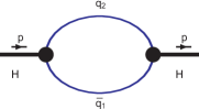
Figure 1: Self-energy diagram for a meson.

The requirement $Z_{H}=0$ implies that the physical state does not contain the bare state and is appropriately described as a bound state. The interaction leads to a dressed physical particle, i.e. its mass and wave function have to be renormalized. The condition $Z_{H}=0$ also effectively excludes the constituent degrees of freedom from the space of physical states. It thereby guarantees the absence of double counting for the physical observable under consideration, the constituents only exist in virtual states.

Therefore, the coupling constants $g_{H}$ of hadrons $H$ are strictly fixed by the requirements of Eq. (8) and do not constitute further free parameters.

IV   One-photon radiative transitions of charmonium states

We consider the dominant one-photon radiative transitions of the charmonium $S$- and $P$-wave states $X=\{J/\psi({{}^{3}}\!S_{1}),\chi_{c0}({{}^{3}}\!P_{0}),\chi_{c1}({{}^{3}}\!P_{1}),h_{c}({{}^{1}}\!P_{1}),\chi_{c2}({{}^{3}}\!P_{2})\}$. The orbitally excited state $h_{c}(3525)$ is included in the considerations despite the large uncertainty in its full decay width.

The latest data on the masses, full decay widths and branching fraction of the dominant radiative decays of the charmonium S- and P-wave states reported in PDG20 are given in Table 1.

Table 1: The charmonium states ${{}^{2S+1}}\!{\it L}_{J}$ and dominant radiative decay modes PDG20 .

State	$J^{PC}$	Interpolating current	Mass (MeV)	Full width ($\Gamma$)	Mode	Fraction ($\Gamma_{i}/\Gamma$)
$\eta_{c}({{}^{1}}\!S_{0})$	$0^{-+}$	$i\bar{q}\,\gamma^{5}q$	2983.9$\pm$0.5	32.0$\pm$0.7 MeV	$\gamma\,\gamma$	(1.58$\pm$0.11) $\cdot 10^{-4}$
$J/\psi({{}^{3}}\!S_{1})$	$1^{--}$	$\bar{q}\,\gamma^{\mu}q$	3096.9$\pm$0.0006	92.9$\pm$2.8 keV	$\gamma\,\eta_{c}$	(1.7$\pm$0.4) $\cdot 10^{-2}$
$\chi_{c0}({{}^{3}}\!P_{0})$	$0^{++}$	$\bar{q}\,Iq$	3414.71$\pm$0.30	10.8$\pm$0.6 MeV	$\gamma\,J/\psi$	(1.40$\pm$0.05) $\cdot 10^{-2}$
$\chi_{c1}({{}^{3}}\!P_{1})$	$1^{++}$	$\bar{q}\,\gamma^{\mu}\gamma^{5}\,q$	3510.67$\pm$0.05	0.84$\pm$0.04 MeV	$\gamma\,J/\psi$	(34.3$\pm$1.0) $\cdot 10^{-2}$
$h_{c}({{}^{1}}\!P_{1})$	$1^{+-}$	$i{\bar{q}}\!\stackrel{{\scriptstyle\leftrightarrow}}{{\partial}}_{\nu}\!\gamma^{5}q$	3525.38$\pm$0.11	0.7$\pm$0.4 MeV	$\gamma\,\eta_{c}$	(51$\pm$6) $\cdot 10^{-2}$
$\chi_{c2}({{}^{3}}\!P_{2})$	$2^{++}$	${\frac{i}{2}}\,{\bar{q}}\left(\gamma^{\mu}\!\!\stackrel{{\scriptstyle\leftrightarrow}}{{\partial}}_{\nu}\!\!+\gamma^{\nu}\!\!\stackrel{{\scriptstyle\leftrightarrow}}{{\partial}}_{\mu}\!\right)q$	3556.17$\pm$0.07	1.97$\pm$0.09 MeV	$\gamma\,J/\psi$	(19.0$\pm$0.5) $\cdot 10^{-2}$

The invariant matrix element for the one-photon radiative transition $X_{1}\to\gamma X_{2}$ reads

$${\cal M}_{X_{1}\to\gamma X_{2}}^{\sigma}=i(2\pi)^{4}\delta^{(4)}(p-q_{1}-q_{2})\,\varepsilon_{X_{1}}\,\varepsilon_{X_{2}}\,\varepsilon_{\gamma\sigma}\,T_{X_{1}\to\gamma X_{2}}^{\sigma}(q_{1},q_{2})\,,$$ (10)

where $\{p,q_{1},q_{2}\}$ and $\{\varepsilon_{X_{1}}\,,\varepsilon_{X_{2}}\,,\varepsilon_{\gamma}\,\}$ are the momenta and polarization vectors of the $X_{1}$, $X_{2}$ and the photon ($\gamma$), correspondingly.

In leading order, the transition amplitude $T_{X_{1}\to\gamma X_{2}}^{\sigma}(q_{1},q_{2})$ in Eq. (10) is described by the triangle and bubble Feynman diagrams shown in Fig. 2.

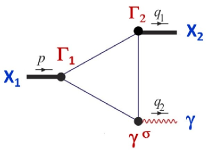
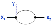
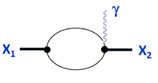
Figure 2: Feynman diagrams contributing in leading order to the dominant one-photon radiative transitions $X_{1}(p)\to\gamma(q_{2})+X_{2}(q_{1})$ of the charmonium states.

Note, each particular diagram in Fig. 2 is not gauge invariant by itself, but the total sum fulfills the gauge invariance requirement:

$$q_{2\sigma}\cdot T^{\rm tot;\sigma}_{X_{1}\to\gamma X_{2}}(q_{1},q_{2})=0\,.$$ (11)

To simplify the calculation we split the contribution of each diagram $T^{\sigma}_{X_{1}\to\gamma X_{2}}(q_{1},q_{2})$ into a part which is gauge invariant $T^{{\rm inv};\sigma}_{X_{1}\to\gamma X_{2}}(q_{1},q_{2})$ and one which is not $T^{{\rm rest};\sigma}_{X_{1}\to\gamma X_{2}}(q_{1},q_{2})$:

$$T^{\sigma}_{X_{1}\to\gamma X_{2}}(q_{1},q_{2})=T^{{\rm inv};\sigma}_{X_{1}\to\gamma X_{2}}(q_{1},q_{2})\,+\,T^{{\rm rest};\sigma}_{X_{1}\to\gamma X_{2}}(q_{1},q_{2})\,.$$ (12)

This separation can be achieved in the following manner. For the $\gamma$-matrix and the four momenta with photon Lorentz index we use the substitutions $\gamma^{\sigma}=\gamma^{\sigma}_{\perp}+q^{\sigma}\!\not\!\!q/q^{2}$ and $p^{\sigma}=p^{\sigma}_{\perp}+q^{\sigma}(p\cdot q)/q^{2}$ where $\gamma^{\sigma}_{\perp}=\gamma^{\sigma}-q^{\sigma}\!\not\!\!q/q^{2}$ and $p^{\sigma}_{\perp}=p^{\sigma}-q^{\sigma}(p\cdot q)/q^{2}$ obey the transversity conditions $\gamma^{\sigma}_{\perp}\cdot q_{\sigma}=0$ and $p^{\sigma}_{\perp}\cdot q_{\sigma}=0$. Expressions for diagrams containing only $\perp$-values are gauge invariant separately. It is easy to show that the remaining terms, which are not gauge invariant, cancel each other in total (see detailed discussion, e.g., in Ref. Faessler:2003yf ). Therefore, it is enough to consider only the sum of the gauge-invariant contributions from all diagrams in Fig. 2. The contributions to the full gauge-invariant amplitude given by the bubble-type diagrams are small and do not exceed the common errors ($\pm 10\%$) of our calculations within the CCQM. Therefore, taking into account the uncertainty of the experimental data in Table 1, we drop the bubble-type diagrams from the consideration without loss in accuracy of our estimates.

The LO amplitude of the charmonium radiative (one-photon) transition described by the gauge-invariant contribution of the triangle diagram in Fig. 2 in our approach reads

$$T_{X_{1}\to\gamma X_{2}}^{{\rm inv};\sigma}(q_{1},q_{2}) \!\!=\!\! g_{X_{1}}g_{X_{2}}e_{c}eN_{c}\!\!\int\!\!\frac{d^{4}k}{(2\pi)^{4}i}\widetilde{\Phi}_{X_{1}}\Big{(}\!\!-\!k^{2}\Big{)}\widetilde{\Phi}_{X_{2}}\Big{(}\!\!-\!\!(k\!+\!\tfrac{1}{2}q_{2})^{2}\Big{)}$$ (13)

$$\!\!\!\cdot\!\!\! {\rm tr}\Big{[}\Gamma_{2}S(\hat{k}+\tfrac{1}{2}\hat{p})\Gamma_{1}\widetilde{S}(\hat{k}-\tfrac{1}{2}\hat{p})\gamma^{\sigma}_{\perp}\widetilde{S}(\hat{k}-\tfrac{1}{2}\hat{p}+\hat{q}_{2})\Big{]},$$

where $e_{c}\!=\!2/3$, $e$ is the electron electric charge; $\Gamma_{1}\!=\!\{\gamma^{\mu},I,\gamma^{\mu}\gamma_{5},\,\stackrel{{\scriptstyle\leftrightarrow}}{{\partial}}_{\nu}\!\!\gamma^{5}\,,i(\gamma^{\mu}\!\!\stackrel{{\scriptstyle\leftrightarrow}}{{\partial}}_{\nu}+\gamma^{\nu}\!\!\stackrel{{\scriptstyle\leftrightarrow}}{{\partial}}_{\mu})/2\}$ for $\{J/\psi,\chi_{c0},\chi_{c1},h_{c},\chi_{c2}\}$ and $\Gamma_{2}\!=\!\{i\gamma^{5},\gamma^{\mu}\}$ for $\{\eta_{c},J/\psi\}$, correspondingly.

As mentioned above, the renormalized couplings $g_{X_{1}}$ and $g_{X_{2}}$ are strictly determined by the self-energy (mass) function of the corresponding charmonia in Eq. (8).

By substituting the Gaussian-type vertices functions and the charm quark propagators in the Fock-Schwinger representation we rewrite the transition amplitude as follows:

$$T_{X_{1}\to\gamma X_{2}}^{{\rm inv};\sigma}(q_{1},q_{2}) \!\!\!=\!\!\! g_{X_{1}}g_{X_{2}}e_{c}eN_{c}\!\!\int\!\!\!\!\intop_{0}^{1}\!\!\!\!\int\!\!d\alpha_{1}\,d\alpha_{2}\,d\alpha_{3}$$ (14)

$$\!\!\cdot\!\! \!\!\int\!\!\frac{d^{4}k}{(2\pi)^{4}i}\exp\left\{\!k^{2}(\alpha_{1}\!+\alpha_{2}\!+\alpha_{3}\!+s_{1}\!+s_{2})+2k^{\nu}R^{\nu}+R_{0}\right\}$$

$$\!\!\!\cdot\!\!\! {\rm tr}\Big{[}\Gamma_{2}(m_{c}+\hat{k}+\tfrac{1}{2}\hat{p})\,\Gamma_{1}(m_{c}+\hat{k}-\tfrac{1}{2}\hat{p})\gamma^{\sigma}_{\perp}(m_{c}+\hat{k}-\tfrac{1}{2}\hat{p}+\hat{q}_{2})\Big{]}\,.$$

Here, $R^{\nu}$ and $R_{0}$ are linear combinations of the external momenta $\{p,q_{1},q_{2}\}$ which also depend on the charmonium size parameters $\{s_{1},s_{2}\}$ as well as the integration variables $\{\alpha_{1},\alpha_{2},\alpha_{3}\}$.

Note, we use the same Gaussian-type vertex function [see Eq. (3)] both for the ground-state and orbitally excited charmonia.

We take the trace for given $\Gamma_{1}$ and $\Gamma_{2}$ and perform an explicit $k$-integration in Eq. (14) while turning the set of Fock-Schwinger parameters into a simplex (see Eq. (6)). Finally we obtain the LO gauge-invariant transition amplitude of the dominant radiative decay of a charmonium state as follows:

$$T_{X_{1}\to\gamma X_{2}}^{{\rm inv}}(q_{1},q_{2})\!\! = \!\!\frac{g_{X_{1}}\,g_{X_{2}}\,e_{c}\,e\,N_{c}}{(2\pi)^{2}}\,\intop_{0}^{1/\lambda^{2}}\!\!\!dt\frac{t^{2}}{(s+t)^{2}}\int\!\!\!\intop_{0}^{1}\!\!\!\int\!\!\!d\alpha_{1}\,d\alpha_{2}\,d\alpha_{3}\,\delta(1-\alpha_{1}-\alpha_{2}-\alpha_{3})$$ (15)

$$\cdot \!\!\!\!f_{\Gamma_{1},\Gamma_{2}}(p,q_{1},q_{2},m_{c},s,t,\alpha_{1},\alpha_{2},\alpha_{3})\cdot\exp\Big{(}\!-\!t\,z_{0}\!+\!\frac{t\,s}{s+t}\,z_{1}\!+\!\frac{s^{2}}{s+t}\,z_{2}\!\Big{)},$$

where

$$z_{0} = m_{c}^{2}-p^{2}\,\alpha_{1}\alpha_{2}-q_{1}^{2}\,\alpha_{2}\alpha_{3}\,,$$

$$z_{1} = p^{2}(\alpha_{1}-\bar{s}_{1}/2)(1/2-\alpha_{2})+q_{1}^{2}(\alpha_{1}-1/2)(\alpha_{1}+\alpha_{2}-\bar{s}_{1}-\bar{s}_{2}/2)\,,$$

$$z_{2} = q_{2}^{2}\bar{s}_{1}\bar{s}_{2}/4\,,$$

$$s_{1} = 1/\Lambda^{2}_{X_{1}}\,,\quad s_{2}=1/\Lambda^{2}_{X_{2}}\,,\quad s=s_{1}+s_{2}\,,\quad\bar{s}_{1}=s_{1}/s\,,\quad\bar{s}_{2}=s_{2}/s.$$

$\Lambda_{X_{1}}$ and $\Lambda_{X_{2}}$ are the size parameters for the in and outgoing charmonia, while $p^{2}=M_{X_{1}}^{2}$, $q_{1}^{2}=M_{X_{2}}^{2}$ have on-mass-shell values. The limit $q_{2}^{2}=0$ corresponds to an outgoing real photon in the radiative decay.

Note, the kernel integrand $f_{\Gamma_{1},\Gamma_{2}}(\ldots)$ in Eq. (15) is formed by the trace operation in Eq. (14), and defines the main structure of the transition amplitude. Below we apply the CCQM to the charmonium S- and P-wave states where explicit expressions for the transition amplitudes are presented.

Transition $J/\psi({}^{3}\!S_{1})\to\gamma\eta_{c}({}^{1}\!S_{0})$

First we consider a typical electromagnetic M1 transition between ground states, from the vector $J/\psi$ ($\Gamma_{1}=\gamma^{\rho}$) to the pseudoscalar $\eta_{c}$ ($\Gamma_{2}=i\gamma^{5}$) by radiating a photon ($\Gamma_{\gamma}=\gamma^{\sigma}$).

For this case we calculate in Eq. (15):

$$f_{\Gamma_{1},\Gamma_{2}}=m_{c}\,\epsilon^{q_{1}q_{2}\rho\sigma}\,,\qquad\epsilon^{q_{1}q_{2}\rho\sigma}\equiv\epsilon^{\mu\nu\rho\sigma}q_{1}^{\mu}q_{2}^{\nu}\,,$$ (16)

where $\epsilon^{\mu\nu\rho\sigma}$ is the four-dimensional antisymmetric Levi-Civita tensor.

Accordingly, the gauge invariant transition amplitude in Eq. (15) takes the form:

$$T^{{\rm inv};\rho\sigma}_{J/\psi\to\gamma\eta_{c}}=g_{J/\psi}\,g_{\eta_{c}}\,C(p^{2},q_{1}^{2},q_{2}^{2})\,\epsilon^{q_{1}q_{2}\rho\sigma}\,,$$ (17)

where the form factor reads:

$$C=\frac{e_{c}eN_{c}m_{c}}{(2\pi)^{2}}\intop_{0}^{1/\lambda^{2}}\!\!\!\frac{dt\,t^{2}}{(s+t)^{2}}\!\!\intop_{0}^{1}\!\!\!\!\int\!\!d\alpha_{1}d\alpha_{2}\,\exp\left\{-t\,z_{0}\!+\!\frac{t\,s}{s+t}\,z_{1}\!+\!\frac{s^{2}}{s+t}\,z_{2}\!\right\}\,,$$ (18)

with $s_{1}=1/\Lambda_{J/\psi}^{2}$, $s_{2}=1/\Lambda_{\eta_{c}}^{2}$, $p^{2}=M^{2}_{J/\psi}$, $q_{1}^{2}=M^{2}_{\eta_{c}}$, $q_{2}^{2}=0$ and $\alpha_{3}=1-\alpha_{1}-\alpha_{2}$.

The renormalized couplings $g_{J/\psi}$ and $g_{\eta_{c}}$ are dimensionless and defined according to Eq. (8) by using the following diagonal parts of the corresponding polarization kernels:

$$g_{J/\psi}\!\! = \!\!\left\{\frac{N_{c}}{3}\Big{(}g_{\mu\nu}-\frac{p_{\mu}\,p_{\nu}}{p^{2}}\Big{)}\!\!\int\!\!\!\frac{d^{4}k}{(2\,\pi)^{4}\,i}\,\widetilde{\Phi}_{J/\psi}^{2}(-k^{2})\,{\rm tr}\left[\gamma_{\mu}\,\widetilde{S}(\hat{k}-\frac{\hat{p}}{2})\,\gamma_{\nu}\,\widetilde{S}(\hat{k}+\frac{\hat{p}}{2})\right]\right\}^{-1/2}\!\!\!\!\!,\,\,\,p^{2}=M^{2}_{J/\psi},$$

$$g_{\eta_{c}}\!\! = \!\!\left\{N_{c}\!\!\int\!\!\!\frac{d^{4}k}{(2\,\pi)^{4}\,i}\,\widetilde{\Phi}_{\eta_{c}}^{2}(-k^{2})\,{\rm tr}\left[\gamma^{5}\,\widetilde{S}(\hat{k}-\frac{\hat{p}}{2})\,\gamma^{5}\,\widetilde{S}(\hat{k}+\frac{\hat{p}}{2})\right]\right\}^{-1/2}\!\!\!\!\!,\quad p^{2}=M^{2}_{\eta_{c}}\,.$$ (19)

Finally, we calculate the fractional one-photon radiative decay width of the vector ground state $J/\psi$ as follows:

$$\Gamma(J/\psi\to\gamma\eta_{c})=\frac{\alpha}{24}\,g_{J/\psi}^{2}\,g_{\eta_{c}}^{2}\,M_{J/\psi}^{3}\,\left(1-\frac{M_{\eta_{c}}^{2}}{M_{J/\psi}^{2}}\right)^{3}\cdot\left[C(M^{2}_{J/\psi},M^{2}_{\eta_{c}},0)\right]^{2}\,,$$ (20)

where $\alpha=e^{2}/4\pi=1/137.036$ is the fine-structure constant.

Transition $\chi_{c0}({{}^{3}}\!P_{0})\to\gamma J/\psi({}^{3}\!S_{1})$

The most general form of the one-photon radiative transition amplitude of the orbitally excited (scalar) charmonium into the vector ground-state reads:

$$T^{{\rm inv};\rho\sigma}_{\chi_{c0}\to\gamma J/\psi}(q_{1},q_{2})=a\,g^{\rho\sigma}+b\,q_{1}^{\rho}\,q_{1}^{\sigma}+c\,q_{1}^{\rho}\,q_{2}^{\sigma}+d\,q_{2}^{\rho}\,q_{1}^{\sigma}+e\,q_{2}^{\rho}\,q_{2}^{\sigma}$$ (21)

with five seemingly independent terms (see, e.g. game09 ).

By taking into account the Lorentz conditions ($q_{1}^{\rho}\cdot\varepsilon_{J/\psi;\rho}=0$, $q_{2}^{\sigma}\cdot\varepsilon_{\gamma;\sigma}=0$) and applying the gauge invariance condition ($q_{2\sigma}\cdot T^{{\rm inv};\rho\sigma}_{\chi_{c0}\to\gamma J/\psi}=0$) one finds that the terms with coefficients $b$, $c$, and $e$ do not contribute while two remaining coefficients are related: $a=-d\,(q_{1}\cdot q_{2})$.

Therefore, the number of independent terms is reduced to one and the gauge-invariant transition amplitude reads

$$T^{{\rm inv};\rho\sigma}_{\chi_{c0}\to\gamma J/\psi}(q_{1},q_{2})=g_{\chi_{c0}}\,g_{J/\psi}\,d(p^{2},q_{1}^{2},q_{2}^{2})\cdot\big{(}q_{1}^{\sigma}q_{2}^{\rho}-g_{\rho\sigma}(q_{1}\!\cdot\!q_{2})\big{)}$$ (22)

resulting in

$$|\varepsilon_{J/\Psi;\rho}\,\varepsilon_{\gamma;\sigma}\,T^{{\rm inv};\rho\sigma}_{\chi_{c0}\to\gamma J/\psi}(q_{1},q_{2})|^{2}=\frac{1}{2}M^{4}_{\chi_{c0}}\big{(}1-M^{2}_{\Psi}/M^{2}_{\chi_{c0}}\big{)}^{2}\,g_{\chi_{c0}}^{2}\,g_{J/\psi}^{2}\,d^{2}\,.$$ (23)

For $\Gamma_{1}=I$ and $\Gamma_{2}=\gamma^{\rho}$ we calculate in Eq. (15):

$$f_{\Gamma_{1},\Gamma_{2}}=m_{c}\,\left(\frac{1}{2}+\frac{t\alpha_{3}+s_{2}/2}{s+t}\right)\,\cdot\big{(}q_{1}^{\sigma}q_{2}^{\rho}-g_{\rho\sigma}(q_{1}\!\cdot\!q_{2})\big{)}$$ (24)

and accordingly, the form factor $d$ reads:

$$d=\frac{e_{c}eN_{c}m_{c}}{(2\pi)^{2}}\intop_{0}^{1/\lambda^{2}}\!\!\!dt\frac{t^{2}}{(s+t)^{2}}\!\!\intop_{0}^{1}\!\!\!\!\int\!\!d\alpha_{1}d\alpha_{2}\left(\frac{1}{2}+\frac{t\alpha_{3}+s_{2}/2}{s+t}\right)e^{-t\,z_{0}+\frac{t\,s}{s+t}\,z_{1}}\,,$$ (25)

where $s_{1}=1/\Lambda_{\chi_{c0}}^{2}$, $s_{2}=1/\Lambda_{J/\psi}^{2}$, $\alpha_{3}=1-\alpha_{1}-\alpha_{2}$, $p^{2}=M^{2}_{\chi_{c0}}$, $q_{1}^{2}=M^{2}_{J/\psi}$ and $q_{2}^{2}=0$.

The renormalized coupling $g_{\chi_{c0}}$ is dimensionless and defined according to Eq. (8) by using the mass function as follows:

$$g_{\chi_{c0}}\!\! = \!\!\left\{N_{c}\int\!\!\!\frac{d^{4}k}{(2\,\pi)^{4}\,i}\,\widetilde{\Phi}_{\chi_{c0}}^{2}(-k^{2})\,{\rm tr}\left[\widetilde{S}(k-\frac{p}{2})\,\widetilde{S}(k+\frac{p}{2})\right]\right\}^{-1/2}\,.$$ (26)

The partial width of the decay $\chi_{c0}\to\gamma J/\psi$ is obtained as follows:

$$\Gamma(\chi_{c0}\to\gamma J/\psi)=\frac{\alpha}{24}g_{\chi_{c0}}^{2}\,g_{J/\psi}^{2}\,M_{\chi_{c0}}^{3}\left(1-\frac{M_{J/\psi}^{2}}{M_{\chi_{c0}}^{2}}\right)^{3}\cdot\left[d(g_{\chi_{c0}},g_{J/\psi},M^{2}_{\chi_{c0}},M^{2}_{J/\psi},0)\right]^{2}\,.$$ (27)

Transition $\chi_{c1}({{}^{3}}\!P_{1})\to\gamma J/\psi({}^{3}\!S_{1})$

The matrix element for the transition $\chi_{c1}\to\gamma J/\psi$ of the excited axial-vector charmonium ($\Gamma_{1}=\gamma^{\mu}\gamma^{5}$) into the vector ground state ($\Gamma_{2}=\gamma^{\rho}$) reads

$${\cal M}_{\chi_{c1}\to\gamma J/\psi}\sim\varepsilon_{\chi_{c1;\mu}}(p)\cdot\varepsilon_{J/\psi;\rho}(q_{1})\cdot\varepsilon_{\gamma;\sigma}(q_{2})\cdot T^{{\rm inv};\mu\rho\sigma}_{\chi_{c1}\to\gamma J/\psi}\,,$$ (28)

where the polarization vectors $\varepsilon_{\chi_{c1}}$, $\varepsilon_{J/\psi}$ and $\varepsilon_{\gamma}$ satisfy transversality, completeness and orthonormality conditions (see, e.g., Ref. bran10ivan17 ).

By taking into account the Lorentz conditions

$$p_{\mu}\,\varepsilon_{\chi_{c1}}^{\mu}=0,\qquad q_{1\rho}\,\varepsilon_{J/\psi}^{\rho}=0,\qquad q_{2\sigma}\,\varepsilon_{\gamma}^{\sigma}=0$$ (29)

and applying the gauge invariance requirement

$$q_{2\sigma}\,T^{{\rm inv};\mu\rho\sigma}_{\chi_{c1}\to\gamma J/\psi}(q_{1},q_{2})=0$$ (30)

we write down the gauge-invariant transition amplitude with four seemingly independent Lorentz structures as follows:

$$T^{{\rm inv};\mu\rho\sigma}_{\chi_{c1}\to\gamma J/\psi}(q_{1},q_{2}) = g_{\chi_{c1}}\,g_{J/\psi}\,\left[\epsilon^{q_{2}\mu\sigma\rho}(q_{1}\cdot q_{2})\,W_{1}+\epsilon^{q_{1}q_{2}\sigma\rho}q_{1}^{\mu}\,W_{2}\right.$$ (31)

$$+ \left.\epsilon^{q_{1}q_{2}\mu\rho}q_{2}^{\sigma}\,W_{3}+\epsilon^{q_{1}q_{2}\mu\sigma}q_{1}^{\rho}\,W_{4}-\epsilon^{q_{1}\mu\sigma\rho}(q_{1}\cdot q_{2})\,W_{4}\right]\,.$$

In accordance with this pattern, we calculate the form factors $W_{1}$, $W_{2}$, $W_{3}$ and $W_{4}$ from Eq. (15) by taking into account definitions $s_{1}=1/\Lambda_{\chi_{c1}}^{2}$, $s_{2}=1/\Lambda_{J/\psi}^{2}$, $\alpha_{3}=1-\alpha_{1}-\alpha_{2}$ and the on-mass-shell conditions $p^{2}=M^{2}_{\chi_{c1}}$, $q_{1}^{2}=M^{2}_{J/\psi}$, $q_{2}^{2}=0$.

These form factors $W_{i}$ are proportional to the dimensionless renormalized coupling $g_{\chi_{c1}}$ which is defined [see Eq. (8)] by using the diagonalized polarization kernel:

$$g_{\chi_{c1}}\!\! = \!\!\left\{\frac{N_{c}}{3}\Big{(}g_{\mu\nu}-\frac{p_{\mu}\,p_{\nu}}{p^{2}}\Big{)}\int\!\!\!\frac{d^{4}k}{(2\,\pi)^{4}\,i}\,\widetilde{\Phi}_{\chi_{c1}}^{2}(-k^{2})\,{\rm tr}\left[\gamma^{\mu}\gamma^{5}\,\widetilde{S}(k-\frac{p}{2})\,\gamma^{\nu}\gamma^{5}\,\widetilde{S}(k+\frac{p}{2})\right]\right\}^{-1/2}\!\!\!\!\!\,.$$ (32)

By using specific symmetry relations between tensors $\epsilon^{\mu\nu\rho\sigma}$ described earlier in dubn10 we can reduce the number of independent Lorentz structures into two as follows:

$$T^{{\rm inv};\mu\rho\sigma}_{\chi_{c1}\to\gamma J/\psi}=g_{\chi_{c1}}\,g_{J/\psi}\,\left[\epsilon^{q_{1}q_{2}\mu\rho}\,q_{2}^{\sigma}\left(W_{1}\!+\!W_{3}\!-\!\frac{q_{1}^{2}}{(q_{1}\,q_{2})}W_{4}\right)\!+\!\epsilon^{q_{1}q_{2}\sigma\rho}\,q_{1}^{\mu}\left(W_{1}\!+\!W_{2}\!-\!W_{4}\!-\!\frac{q_{1}^{2}}{(q_{1}\,q_{2})}W_{4}\right)\right]\,.$$ (33)

We further introduce the following helicity amplitudes (see, dubn10 )

$$H_{L} = ig_{\chi_{c1}}\,g_{J/\psi}\,\frac{M_{\chi_{c1}}^{2}}{M_{J/\psi}}|\vec{q}_{2}|^{2}\Big{[}W_{1}+W_{3}-\frac{M^{2}_{J/\psi}}{M_{\chi_{c1}}|\vec{q}_{2}|}W_{4}\Big{]}\,,\qquad|\vec{q}_{2}|=\frac{M_{\chi_{c1}}^{2}-M^{2}_{J/\psi}}{2M_{\chi_{c1}}}\,,$$

$$H_{T} = -ig_{\chi_{c1}}\,g_{J/\psi}\,M_{\chi_{c1}}|\vec{q}_{2}|^{2}\Big{[}W_{1}+W_{2}-\Big{(}1+\frac{M^{2}_{J/\psi}}{M_{\chi_{c1}}|\vec{q}_{2}|}\Big{)}\,W_{4}\Big{]}\,.$$ (34)

Then, the partial decay width of the axial-vector charmonium $\chi_{c1}({{}^{3}}\!P_{1})$ reads

$$\Gamma(\chi_{c1}\to\gamma J/\Psi)=\frac{g_{\chi_{c1}}^{2}\,g_{J/\psi}^{2}\,}{12\pi}\frac{|\vec{q}_{2}|}{M_{\chi_{c1}}^{2}}\Big{(}|H_{L}|^{2}+|H_{T}|^{2}\Big{)}\,.$$ (35)

Transition $h_{c}({{}^{1}}\!P_{1})\to\gamma\eta_{c}({{}^{1}}\!S_{0})$

As mentioned above, we also consider the one-photon radiative transition of the orbitally excited charmonium state $h_{c}(3525)$ despite the large uncertainty in the full decay width (see Table I).

By substituting the matrices $\Gamma_{1}=k^{\mu}\gamma^{5}$ in Eq. (14) and $\Gamma_{2}=\gamma^{\rho}$ we obtain the gauge invariant amplitude of the transition $h_{c}\to\gamma\eta_{c}$ as follows:

$$T^{{\rm inv};\rho\sigma}_{h_{c}\to\gamma\eta_{c}}(q_{1},q_{2})=g_{h_{c}}\,g_{\eta_{c}}\,{\emph{h}}(p^{2},q_{1}^{2},q_{2}^{2})\cdot(q_{2}^{\rho}q_{1}^{\sigma}-g^{\rho\sigma}(q_{1}\cdot q_{2})\big{)}\,,$$ (36)

where the form factor h is calculated by using Eq. (14) in a similar way as described in the previous subsections.

In contrast to $g_{\eta_{c}}$ the renormalized coupling $g_{h_{c}}$ is dimensional ($\sim$ GeV^-1) and defined [see Eq. (8)] by using the diagonalized polarization kernel:

$$g_{h_{c}}\!\! = \!\!\left\{\frac{N_{c}}{3}\Big{(}g_{\mu\nu}-\frac{p_{\mu}\,p_{\nu}}{p^{2}}\Big{)}\int\!\!\!\frac{d^{4}k}{(2\,\pi)^{4}\,i}\,\widetilde{\Phi}_{h_{c}}^{2}(-k^{2})\,{\rm tr}\left[k^{\mu}\gamma^{5}\,\widetilde{S}(k-\frac{p}{2})\,k^{\nu}\gamma^{5}\,\widetilde{S}(k+\frac{p}{2})\right]\right\}^{-1/2}\!\!\!\!.$$ (37)

For the square of the invariant matrix element we have

$$|{\cal M}_{h_{c}\to\gamma\eta_{c}}|^{2}\sim|\varepsilon_{h_{c};\rho}\,\varepsilon_{\gamma;\sigma}\,T^{{\rm inv};\rho\sigma}_{h_{c}\to\gamma\eta_{c}}(q_{1},q_{2})|^{2}=\frac{1}{2}g_{h_{c}}^{2}\,g_{\eta_{c}}^{2}\,M^{4}_{h_{c}}\big{(}1-M^{2}_{\eta_{c}}/M^{2}_{h_{c}}\big{)}^{2}\cdot|{\emph{h}}(p^{2},q_{1}^{2},q_{2}^{2})|^{2}$$ (38)

with $s_{1}=1/\Lambda_{h_{c}}^{2}$, $s_{2}=1/\Lambda_{J/\psi}^{2}$, $p^{2}=M^{2}_{h_{c}}$, $q_{1}^{2}=M^{2}_{J/\psi}$ and $q_{2}^{2}=0$.

The fractional decay width of the excited charmonium state $h_{c}({{}^{1}}\!P_{1})$ reads

$$\Gamma(h_{c}\to\gamma\eta_{c})=\frac{\alpha\,g_{h_{c}}^{2}\,g_{\eta_{c}}^{2}\,}{24\,(1+2S)}M_{h_{c}}^{3}\left(1-\frac{M_{\eta_{c}}^{2}}{M_{h_{c}}^{2}}\right)^{3}\cdot|{\emph{h}}(M_{h_{c}}^{2},M_{\eta_{c}}^{2},0)|^{2}\,,$$ (39)

with the spin value $S=1$.

Transition $\chi_{c2}({{}^{3}}\!P_{2})\to\gamma J/\psi({}^{3}\!S_{1})$

The polarization vector $\varepsilon_{\mu\nu}^{(\lambda)}$ (below we denote as $\varepsilon^{\mu\nu}_{\chi_{c2}}$) of the tensor meson $\chi_{c2}$ satisfies the symmetry, transversality, tracelessness, orthonormality and completeness conditions:

$$\varepsilon^{(\lambda)}_{\mu\nu}(p)=\varepsilon^{(\lambda)}_{\nu\mu}(p),\qquad\varepsilon^{(\lambda)}_{\mu\nu}(p)\,p^{\mu}=0,\qquad\varepsilon^{(\lambda)}_{\mu\nu}(p)\,g^{\mu\nu}=0,\qquad\varepsilon^{\dagger\,(\lambda)}_{\mu\nu}\varepsilon^{(\lambda^{\prime})\,\mu\nu}=\delta_{\lambda\lambda^{\prime}},$$

$$\sum\limits_{\lambda=0,\pm 1,\pm 2}\!\!\!\varepsilon^{(\lambda)}_{\mu\nu}\varepsilon^{\dagger\,(\lambda)}_{\alpha\beta}=\frac{1}{2}\left(\bar{g}_{\mu\alpha}\,\bar{g}_{\nu\beta}+\bar{g}_{\mu\beta}\,\bar{g}_{\nu\alpha}\right)-\frac{1}{3}\,\bar{g}_{\mu\nu}\,\bar{g}_{\alpha\beta}\equiv\widetilde{g}_{\mu\nu\alpha\beta},\quad\bar{g}_{\mu\nu}\equiv-g_{\mu\nu}+\frac{p_{\mu}\,p_{\nu}}{p^{2}}\,.$$ (40)

For the gauge invariant amplitude of the transition $\chi_{c2}\to\gamma J/\psi$ we substitute the matrices $\Gamma_{1}=\gamma^{\mu}k^{\nu}\!+\!\gamma^{\nu}k^{\mu}$ and $\Gamma_{2}=\gamma^{\rho}$ into Eq. (14) and obtain

$$T^{{\rm inv};\mu\nu\rho\sigma}_{\chi_{c2}\to\gamma J/\psi}(q_{1},q_{2}) \!\!=\!\! g_{\chi_{c2}}\,g_{J/\psi}\,\left\{A\cdot\Big{(}g^{\mu\rho}\Big{[}g^{\sigma\nu}(q_{1}\cdot q_{2})-q_{1}^{\sigma}\,q_{2}^{\nu}\Big{]}+g^{\nu\rho}\Big{[}g^{\sigma\mu}(q_{1}\cdot q_{2})-q_{1}^{\sigma}\,q_{2}^{\mu}\Big{]}\Big{)}\right.$$ (41)

$$\!\!+\!\! \left.B\cdot\Big{(}g^{\sigma\rho}\Big{[}q_{1}^{\mu}\,q_{2}^{\nu}+q_{1}^{\nu}\,q_{2}^{\mu}\Big{]}-g^{\mu\sigma}q_{1}^{\nu}\,q_{2}^{\rho}-g^{\nu\sigma}q_{1}^{\mu}\,q_{2}^{\rho}\Big{)}\right\}\,,$$

where the two independent form factors $A(g_{\chi_{c2}},g_{J/\psi},p^{2},q_{1}^{2},q_{2}^{2})$ and $B(g_{\chi_{c2}},g_{J/\psi},p^{2},q_{1}^{2},q_{2}^{2})$ are determined by Eq. (15) with $s_{1}=1/\Lambda_{\chi_{c2}}^{2}$, $s_{2}=1/\Lambda_{J/\psi}^{2}$, $p^{2}=M^{2}_{\chi_{c2}}$, $q_{1}^{2}=M^{2}_{J/\psi}$ and $q_{2}^{2}=0$.

The renormalized coupling of the tensor meson is defined [see Eq. (8)] as follows:

$$g_{\chi_{c2}}\!\! = \!\!\left\{\frac{\widetilde{g}_{\mu\nu\rho\sigma}}{5}\,\!\!\!\int\!\!\!\!\frac{d^{4}k}{(2\,\pi)^{4}\,i}\,\widetilde{\Phi}_{\chi_{c2}}^{2}(-k^{2})\,{\rm tr}\left[\left(\gamma^{\mu}k^{\nu}\!+\!\gamma^{\nu}k^{\mu}\right)\widetilde{S}(k-\frac{p}{2})\left(\gamma^{\rho}k^{\sigma}\!+\!\gamma^{\sigma}k^{\rho}\right)\widetilde{S}(k+\frac{p}{2})\right]\right\}^{-1/2}\,$$ (42)

with dimension of ($\sim$ GeV^-1).

For the square of the invariant matrix element for the radiative transition of the tensor charmonium $\chi_{c2}\to\gamma J/\Psi$ we obtain

$$|{\cal M}_{\chi_{c2}\to\gamma J/\psi}|^{2}\sim|\varepsilon_{\chi_{c2};\mu\nu}\varepsilon_{J/\Psi;\rho}\,\varepsilon_{\gamma;\sigma}\,T^{{\rm inv};\mu\nu\rho\sigma}_{\chi_{c2}\to\gamma J/\psi}(q_{1},q_{2})|^{2}\!=\!g_{\chi_{c2}}^{2}\,g_{J/\psi}^{2}\,M_{\chi_{c2}}^{4}\big{(}C_{A}\!\cdot\!A^{2}\!+\!C_{AB}\!\cdot\!A\!\cdot\!B\!+\!C_{B}\!\cdot\!B^{2}\big{)}\,,$$ (43)

where the numerical constants $C_{A}$, $C_{AB}$ and $C_{B}$ are defined through the meson masses as follows:

$$C_{A} = \frac{1}{\xi}\left(\frac{1}{4}+\frac{7}{3}\xi-\frac{31}{6}\xi^{2}+\frac{7}{3}\xi^{3}+\frac{1}{4}\xi^{4}\right)=0.1957,\qquad\xi=M_{J/\psi}^{2}/M_{\chi_{c2}}^{2}=0.7584,$$

$$C_{AB} = -\frac{1}{\xi}\left(\frac{1}{2}-\frac{1}{3}\xi-2\xi^{2}+3\xi^{3}-\frac{7}{6}\xi^{4}\right)=-0.02576,$$ (44)

$$C_{B} = \frac{1}{\xi}\left(\frac{1}{4}-\frac{2}{3}\xi+\frac{1}{6}\xi^{2}+\xi^{3}-\frac{13}{12}\xi^{4}+\frac{1}{3}\xi^{5}\right)=0.00226\,.$$

The fractional decay width of the one-photon radiative transition of the tensor charmonium excitation $\chi_{c2}$ reads:

$$\Gamma(\chi_{c2}\to\gamma J/\psi)=\frac{\alpha\,g_{\chi_{c2}}^{2}\,g_{J/\psi}^{2}\,}{4(1\!+\!2S)}\,M_{\chi_{c2}}^{3}\left(1-\frac{M_{J/\psi}^{2}}{M_{\chi_{c2}}^{2}}\right)\cdot\big{(}C_{A}\!\cdot\!A^{2}\!+\!C_{AB}\!\cdot\!A\!\cdot\!B\!+\!C_{B}\!\cdot\!B^{2}\big{)}$$ (45)

with spin value $S=2$.

V   Numerical results

According to the CCQM the hadronic field is coupled to a nonlocal quark current by the interaction Lagrangian described in Eq. (1), where the nonlocal vertex function in Eq. (3) characterizes the quark distribution inside the hadron. The vertex function $\widetilde{\Phi}_{H}\left(-p^{2}\right)$ is unique for the given hadron and each hadron has its own adjustable parameter $\Lambda_{H}$, which can be related to the hadron ’size’. The fixed values of the “size” parameters of various hadrons differ in the CCQM but for most cases a pattern can be traced - the heavier a hadron, the larger its “size”.

On the other hand, the charmonium members under consideration have the same quark content ($c\bar{c}$) and possess physical masses in a relative narrow interval $\sim 3\div 3.5$ GeV. Therefore, for this specific case we use the ansatz that the charmonium ’size’ is proportional to its physical mass, i.e., $\Lambda_{X}=\varrho\!\cdot\!\!M_{X}$ with a constant $\varrho>0$.

Subsequently, we introduce one common and adjustable “slope” parameter:

$$\varrho\equiv\Lambda_{X}/M_{X}\,,$$ (46)

instead of six separate ’size’ parameters $\Lambda_{X}=\{\Lambda_{\eta_{c}},\Lambda_{J/\psi},\Lambda_{\chi_{c0}},\Lambda_{\chi_{c1}},\Lambda_{h_{c}},\Lambda_{\chi_{c2}}\}$ to describe the quark distribution inside the charmonia.

We further use the charmonium vertex function defined as:

$$\widetilde{\Phi}_{X}\left(-p^{2}\right)=\exp\left(\frac{1}{\varrho^{2}}\!\cdot\!\frac{p^{2}}{M_{X}^{2}}\right)$$ (47)

instead of the conventional one given in Eq. (3).

In doing so, we keep the central values of the basic CCQM parameters represented in Eq. (7). Namely, we use the universal infrared cutoff parameter $\lambda=0.181$ GeV and the constituent charm quark mass in the range of $\pm 10\%$ around $m_{c}=1.67$ GeV.

For the numerical evaluation on the charmonium states we vary the fully adjustable parameter $\varrho>0$ to fit the latest experimental data on radiative charmonium decays reported by the PDG PDG20 .

1. First we calculate the renormalization couplings $g_{H}$ of the hadrons which play an important role in the CCQM by excluding the constituent degrees of freedom from the space of physical states. They are strictly fixed by the compositeness requirements expressed in Eq. (8) and do not constitute further free parameters, although keep indirect dependencies on the basic model parameters. The renormalized couplings of the charmonium ground-states and first orbital excitations calculated in dependence on the “slope” parameter $\varrho$ for $m_{c}=1.80$ GeV are shown in Fig. 3. The renormalization couplings $g_{X}$ decrease monotonically, a larger slope for $\varrho\leq 1$ and more moderately for larger values.

2. Having calculated the renormalization couplings $g_{X}$ we are able to estimate the partial widths of the dominant one-photon radiative decays of the orbitally excited ($\emph{l}=1$) charmonium states $\chi_{cJ},~{}(J=\{0,1,2\})$ by using Eqs. (27), (35) and (45) to find the optimal model value of the “slope” parameter $\varrho>0$. The dependencies of the partial widths $\chi_{c0}$, $\chi_{c1}$ and $\chi_{c2}$ on the “slope” parameter $\varrho$ are shown in Fig. 4 for a fixed value of the charm quark mass $m_{c}=1.80$ GeV. We conclude that our theoretical estimates fit the corresponding experimental data only in the narrow interval $\varrho\in[0.47\div 0.50]$.

3. The dependencies of the charmonium partial decay widths $\Gamma_{X}$ on the charm quark mass $m_{c}$ for fixed values of the “slope” parameter $\varrho=0.485$ are depicted in Fig. 5. The best fits of our theoretical estimates to the corresponding experimental data occur around $m_{c}=1.80$ GeV.

Having fixed the model parameter $m_{c}=1.80$ GeV we are able to calculate the partial widths of the dominant one-photon radiative decays of the ground ($J/\psi\to\gamma\eta_{c}$) and orbitally excited ($h_{c}\to\gamma J\psi$) in dependence on $\varrho$, shown in Fig. 6 together with the curves curves for $\chi_{cJ},~{}J=\{0,1,2\}$.

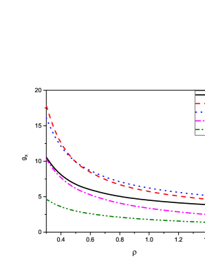
Figure 3: The renormalized couplings of the charmonium ground-states and first orbital excitations calculated in dependence on the slope parameter $\varrho$.

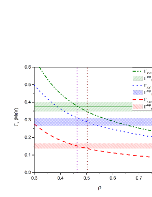
Figure 4: Partial decay widths of the dominant one-photon radiative decays of the orbitally excited ($\emph{l}=1$) charmonium states $\chi_{cJ},~{}J=\{0,1,2\}$ in dependence on the slope parameter $\varrho$ for a fixed c-quark mass $m_{c}=1.80$ GeV. The shaded bands with central horizontal solid lines correspond to the latest experimental data with given error bars.

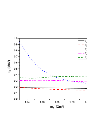
Figure 5: Theoretical estimates of the charmonium partial decay widths $\Gamma_{X}$ in dependence on the charm quark mass $m_{c}$ for fixed values of the slope parameter $\varrho=0.485$.

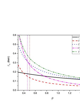
Figure 6: Partial decay widths of the dominant one-photon radiative decays of the charmonium ground $J/\psi$ and orbitally excited ($\emph{l}=1$) states $\chi_{cJ},~{}J=\{0,1,2\},h_{c}$ in dependence on the slope parameter $\varrho$ for fixed c-quark mass $m_{c}=1.80$ GeV. The vertical dotted lines indicate the optimal $\varrho$-interval from the fit of $\chi_{cJ}$ one-photon decays.

Finally by fitting the latest experimental data PDG20 on the partial widths of the dominant one-photon radiative decay of the orbitally excited charmonium states $\chi_{c0}$, $\chi_{c1}$ and $\chi_{c2}$ we fix the optimal values of model parameters as follows:

 $$\lambda$$    

 0.181  GeV  1.80  GeV  0.485

(48)

Note, the adjusted value of the ’slope’ parameter $\varrho$ is common to all charmonium states under consideration and is about 1/2. Subsequently, the conventional ’size’ parameters of these charmonia would be nearly half of their physical masses. The refitted constituent c-quark mass value in Eq. (48) exceeds the central basic value in Eq. (7) within the allowed $\sim 8\%$ deviation.

Our theoretical values for the fractional widths of the dominant one-photon radiative decay of the S- and P-wave charmonia in comparison with some recent theoretical predictions brus2020 ; Becirevic:2012dc ; weijun2016 and experimental data PDG20 are shown in Table 2.

Note, the full decay width of the charmonium state $h_{c}({{}^{1}}\!P_{1})(3525)$ shown in Table 1 is experimentally measured but with a large uncertainty (more than $\pm 50\%$) while the partial decay width of the radiative decay is detected more accurately.

For the experimental value of $\Gamma(h_{c}\to\gamma\eta_{c})$ given in Table 2 we have used the latest data for the full decay width of $h_{c}$ and the corresponding fraction $\Gamma_{i}/\Gamma$ reported in PDG20 and shown in Table 1.

Table 2: Some theoretical predictions of the partial widths (in units of keV) of the dominant radiative decay of the charmonium states below the $D{\bar{D}}$ threshold in comparison with recent data.

$J^{PC}$	Radiative decay	${}^{CCQM}_{\lambda=0.181}$	${}^{CCQM}_{~{}~{}\lambda\to 0}$	Exp . PDG20	p/m brus2020	LWL brus2020	Becirevic:2012dc	weijun2016
$1^{--}$	$\Gamma(J/\psi\to\gamma\eta_{c}$)	1.771	1.771	1.58 $\pm$ 0.43	-	-	2.64(11)	1.25
$0^{++}$	$\Gamma(\chi_{c0}\to\gamma J/\psi)$	142.0	142.0	151 $\pm$ 14	118	128	-	128
$1^{++}$	$\Gamma(\chi_{c1}\to\gamma J/\psi)$	296.7	297.0	288 $\pm$ 22	315	266	-	275
$1^{+-}$	$\Gamma(h_{c}\to\gamma\eta_{c})$	290.8	290.7	357 $\pm$ 270	-	-	720(50)(20)	587
$2^{++}$	$\Gamma(\chi_{c2}\to\gamma J/\psi)$	358.1	356.7	374 $\pm$ 27	419	353	-	467

As mentioned in Sec. II, the uncertainties of our basic model parameters, estimated renormalization couplings and form factors are about $10\%$, while the branching fractions are proportional to the square of these values. We therefore expect that the uncertainties of our calculation of the partial widths in Table 2 do not not exceed more than a few percent.

Concluding this section, we have fixed our model parameters $m_{c}$ and $\varrho$ by fitting the latest data in PDG20 on the partial decay widths of the one-photon radiative decays of the orbitally excited charmonium states $\chi_{c0}$, $\chi_{c1}$ and $\chi_{c2}$. By using these fixed parameters, we have calculated $\Gamma(J/\psi\to\gamma\eta_{c})$ and $\Gamma(h_{c}\to\gamma\eta_{c})$.

VI   Deconfinement limit $\lambda\to 0$

The infrared cutoff parameter introduced in the CCQM plays an important role [see, e.g., Eq. (6)]. It leads to the removal of possible threshold singularities corresponding to the creation of free quarks, and is taken to be universal ($\lambda=0.181$ GeV) for all physical processes. However, in some specific cases these singularities do not appear. Particularly, the fixed value ($m_{c}=1.80$ GeV) of the constituent charm quark mass obeys the condition $M_{X}<2m_{c}$ for all charmonium states under consideration and the initial integral in Eq. (5) converges and we can evaluate it for the full integration range $t\in[0,\infty)$ with $\lambda\to 0$ in Eq. (6).

The dependencies of the renormalized couplings $g_{X}$ and the one-photon radiative partial decay widths $\Gamma_{X}$ of the charmonium states on the upper integration bound $1/\lambda^{2}$ is presented in Fig. 7. The renormalized couplings and partial decay widths depicted in Fig. 7 do not change for $1/\lambda^{2}>20$ GeV^-2 while the CCQM universal confinement parameter $\lambda=0.181$ GeV corresponds to $1/\lambda^{2}=30.52$ GeV^-2. Therefore, our theoretical estimates for the renormalization couplings and fractional widths of the dominant one-photon radiative decay of the charmonium states shown in Table 2 remain unchanged in the deconfinement limit $\lambda\to 0$.

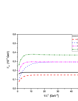
Figure 7: Dependence of the renormalized couplings $g_{X}$ and the one-photon radiative partial decay widths $\Gamma_{X}$ of the charmonium states on the infrared cutoff parameter $1/\lambda^{2}$.

VII   Discussion

VII.1 $J/\psi({}^{3}\!S_{1})\to\gamma\eta_{c}({}^{1}\!S_{0})$

Nowadays, discrepancies still exist between theoretical predictions and the data on the transition $J/\psi\to\gamma\eta_{c}(1S)$.

Particularly, the nonrelativistic potential model Swanson:2005 and the Coulomb gauge approach Guo:2014zva give a partial width of $\Gamma[J/\psi\rightarrow\gamma\eta_{c}]\simeq 2.9$ keV, almost twice as large as the present average data $\Gamma^{\rm exp}(J/\psi\to\gamma\eta_{c})\simeq 1.58\pm 0.37$ keV PDG20 .

Lattice QCD simulations for the hadronic matrix elements Becirevic:2012dc relevant to the radiative $J/\psi\to\gamma\eta_{c}$ and $h_{c}\to\gamma\eta_{c}$ decays have been performed by using the twisted mass QCD action with light dynamical quarks ($N_{\rm f}=2$) for several small lattice spacings. The authors smoothly extrapolated the relevant form factors at four lattice spacings to the continuum limit. For the radiative decay $J/\Psi\to\gamma\eta_{c}$ the lattice simulation computes a decay rate $\Gamma(J/\psi\to\gamma\eta_{c})=2.64(11)(3)$ keV Becirevic:2012dc that is obviously larger than the recent data PDG20 .

Recently, the radiative decays of the charmonium states $J/\psi$, $h_{c}(1P)$ and $\chi_{cJ}(1P)$ have been studied within a constituent quark model. The predicted partial decay width $\Gamma(J/\psi\to\gamma\eta_{c})\simeq 1.25$ keV weijun2016 is significantly (about 22$\%$) lower than the central value of the present data PDG20 .

According to our calculation, the partial decay width of the transition $J/\psi({}^{3}\!S_{1})\to\gamma\eta_{c}({}^{1}\!S_{0})$ in Eq. (20) is proportional to $\alpha\cdot(M_{J/\psi}-M_{\eta_{c}})^{3}\cdot|C(...)|^{2}$. Hereby, we note that the form factor $C$ in Eq. (18) is of order $m_{c}(1/m_{c}^{2}+1/M_{J/\psi}^{2}+1/M_{\eta_{c}}^{2})$ and $m_{c}\sim M_{J/\psi}/2\sim M_{\eta_{c}}/2$. Obviously, the transition rate of $J/\psi\to\gamma\eta_{c}(1S)$ is strongly suppressed by the factor $(M_{J/\psi}-M_{\eta_{c}})^{3}/m_{c}^{2}$.

Our calculation within the CCQM for the partial decay width (see Table II)

$$\Gamma(J/\psi\to\gamma\eta_{c})=1.77\ {\rm keV}$$ (49)

slightly (about 12$\%$) exceeds the average value of the recent data PDG20 .

VII.2 $h_{c}({{}^{1}}\!P_{1})\to\gamma\eta_{c}({{}^{1}}\!S_{0})$

The charmonium state $h_{c}(1P)$ has been discerned from the experimental background only recently, the CLEO succeeded to isolate this state Rosner:2005ry . Only a few decay modes of the $h_{c}$ are observed. Due to its negative $C$-parity, the dominant decay mode is $h_{c}(1P)\to\gamma\eta_{c}(1S)$ with a branching fraction of $(51\pm 6)\%$ Rosner:2005ry ; Dobbs:2008ec ; PDG20 .

There are some discrepancies between the different model predictions for $\Gamma[h_{c}(1P)\to\gamma\eta_{c}]$. A constituent quark model prediction for the partial decay width weijun2016 $\Gamma(h_{c}(1P)\to\gamma\eta_{c})\simeq 587$ keV is consistent with data within its large uncertainties PDG20 but much smaller than the predictions from the relativistic quark model Ebert:2003 and lattice QCD Dudek:2006ej .

A recent lattice calculation gives a larger width of $\Gamma(h_{c}\to\gamma\eta_{c})=720(50)(20)$ keV Becirevic:2012dc . A similar result was also obtained with a light front quark model Ke:2013zs . Both predictions are obviously much larger than the data PDG20 .

Our calculation within the CCQM for the partial decay width reads (see Table II)

$$\Gamma(h_{c}\to\gamma\eta_{c})=0.291\ {\rm MeV}\,.$$ (50)

The present world data for the full decay width of the charmonium state $h_{c}({{}^{1}}\!P_{1})(3525)$ cannot be used to test the various predictions due to their large uncertainties PDG20 . On the other hand, the fractional width for the one-photon radiative decay of $h_{c}({{}^{1}}\!P_{1})(3525)$ is detected more accurately PDG20 . Therefore, by combining the latest value for the fractional width of PDG20 with our estimate in Eq. (50) we may calculate the ’theoretical full decay width’ for $h_{c}$ as follows:

$$\Gamma^{\rm theor}_{h_{c}}\simeq(0.57\pm 0.12)\ {\rm MeV}\,.$$ (51)

Hereby, we admitted a relevant $\sim 10\%$ uncertainty for $\Gamma(h_{c}\to\gamma\eta_{c})$. Compared with data $\Gamma^{\rm exp}_{h_{c}}\simeq(0.7\pm 0.4)$ MeV PDG20 , the prediction in Eq. (51) is located in a more narrow interval.

VII.3 Triplet $\chi_{cJ}({{}^{3}}\!P_{J})\to\gamma J/\psi({}^{3}\!S_{1})$

Recently, a Cornell potential model has been used to study electromagnetic transitions $\chi_{cJ}(1P)\to\gamma J/\psi$ in charmonium brus2020 . The absence of any momentum dependence in the potential allowed for a complete factorization of the heavy quarkonium mass ($m_{c}$) dependence in the calculation of the electromagnetic decay widths in the $\sim p_{c}/m_{c}$ and long-wavelength (LWL) approximations. The calculated decay widths $\Gamma_{p/m}^{(II)}$ and $\Gamma_{LWL}^{(II)}$ in brus2020 are shown in Table 2 in comparison with our present results. Hereby, the effective charm-quark mass parameter, at least for the description of the low lying charmonium states, is constrained to be around $1.840$ GeV. Estimates of $\Gamma(\chi_{c0,c1,c2}(1P)\to\gamma J/\psi)$ reported in weijun2016 with a constituent quark model differ from the average data PDG20 (see Table 2). Some studies on the radiative transition properties of $\chi_{c0,c1}(1P)$ were carried out in Lattice QCD as well Dudek:2006ej ; Chen:2011kpa , however, good descriptions are still not obtained due to some technical problems.

Nowadays, discrepancies still remain between the different model predictions for the partial decay widths $\Gamma(\chi_{cJ}(1P)\to\gamma J/\psi)$ of the charmonium triplet $\chi_{c0,c1,c2}$.

Our calculations for the central values of the partial decay widths (see Table II) read

$$\Gamma(\chi_{c0}(1P)\to\gamma J/\psi)\!\! = \!\!142.0\,{\rm keV}\,,$$

$$\Gamma(\chi_{c1}(1P)\to\gamma J/\psi)\!\! = \!\!296.7\,{\rm keV}\,,$$

$$\Gamma(\chi_{c2}(1P)\to\gamma J/\psi)\!\! = \!\!358.1\,{\rm keV}$$ (52)

and are close to the recent LHCb data  PDG20 .

VIII   Summary

The dominant one-photon radiative transitions of the charmonium $S$- and $P$-wave states have been studied within the CCQM. In doing so, the transition amplitudes have been described by the leading-order triangle diagrams. We neglect the subleading bubble diagrams since their small contributions are comparable to the common model error ($\sim\pm 10\%$). The gauge invariant transition amplitudes have been expressed by using either the conventional Lorentz structures, or the helicity amplitudes, where it was effective.

We used the basic model parameters for the global infrared cutoff ($\lambda=0.181$ GeV) and the constituent c-quark mass ($m_{c}=1.80$ GeV which deviates $\sim 7\%$ from the central model value). We additionally introduced only one adjustable parameter $\varrho>0$ common to the charmonium states $\eta_{c}({}^{1}\!S_{0})$, $J/\psi({}^{3}\!S_{1})$, $\chi_{c0}({{}^{3}}\!P_{0})$, $\chi_{c1}({{}^{3}}\!P_{1})$, $h_{c}({{}^{1}}\!P_{1})$, and $\chi_{c2}({{}^{3}}\!P_{2})$ to describe the quark distribution inside the hadron. This dimensionless parameter indicates the ratio between the charmonium size parameter and its physical mass.

The renormalization couplings $g_{X}$ of the charmonium states play an important role in the CCQM by excluding the constituent degrees of freedom from the space of physical states. They are strictly fixed by the compositeness requirements ($Z_{H}=0$) and further eliminated as free parameters, although keep indirect dependencies on the basic model parameters. We have analyzed the behavior of $g_{X}$ in dependence on $\varrho$. The couplings $g_{X}$ decrease fast for $\varrho\leq 0.8$ and slowly for larger values.

The optimal value of the only adjustable parameter $\varrho$ has been found by fitting the latest data for the partial widths of the one-photon radiative decays of the charmonium triplet $\chi_{cJ}({{}^{3}}\!P_{J}),~{}J=\{0,1,2\}$. Note, the optimal value $\varrho=0.485$ is close to one half and common to all charmonium states under consideration. Then, we calculated fractional widths for the states $J/\psi({}^{3}\!S_{1})$ and $h_{c}({{}^{1}}\!P_{1})$. The results are in agreement with the latest data.

By using the latest partial decay data from PDG2020 PDG20 and our estimated partial decay width for $h_{c}({{}^{1}}\!P_{1})$ we calculate reversely the theoretical ’full decay width’ $\Gamma^{\rm theor}_{h_{c}}\simeq(0.57\pm 0.12)$ MeV that may be compared to $\Gamma^{\rm exp}_{h_{c}}\simeq(0.7\pm 0.4)$ MeV PDG20 .

The infrared cutoff parameter $\lambda$ plays the central role in the CCQM by removing possible threshold singularities corresponding to the creation of free quarks, and is taken to be universal ($\lambda=0.181$ GeV) for all physical processes. However, the fixed charm-quark mass value ($m_{c}=1.80$ GeV) excludes any appearance of branch points due to the mass relations $M_{X}<2m_{c}$ valid for charmonium states under consideration. This allowed us to repeat our calculations by decreasing $\lambda$ gradually close to the deconfinement limit $\lambda\to 0$. Our results obtained for $\lambda=0.181$ GeV changed insignificantly and converged to their limits for $1/\lambda^{2}>20$ GeV^-2 or $\lambda<0.220$ GeV. For this charmonium states our theoretical calculations performed within the CCQM remain unchanged even in the infrared deconfinement limit.

- (1) J. J. Aubert et al. (E598 Collaboration), Phys. Rev. Lett. 33, 1404 (1974).
- (2) J. E. Augustin et al. (SLAC-SP-017Collaboration), Phys. Rev. Lett. 33, 1406 (1974).
- (3) M. Ablikim et al. (BESIII Collaboration), Phys. Rev. D 99, 012015 (2019); R. Aaij et al. (LHCb Collaboration), Phys. Rev. D 92, 112009 (2015); M. Ablikim et al. (BESIII Collaboration), Phys. Rev. Lett. 115, 221805 (2015); A. Zupanc et al. (Belle Collaboration), Phys. Rev. Lett. 113, 042002 (2014); T. Xiao, S. Dobbs, A. Tomaradze, and K. K. Seth, Phys. Lett. B 727, 366 (2013).
- (4) J. L. Rosner et al. (CLEO Collaboration), Phys. Rev. Lett. 95, 102003 (2005).
- (5) M. Ablikim et al. (The BESIII Collaboration), Phys. Rev. Lett. 104, 132002 (2010).
- (6) R. Aaij et al. (LHCb Collaboration), Phys. Lett. B 714, 215 (2012).
- (7) R. Aaij et al. (LHCb Collaboration), production at TeV, JHEP 10, 115 (2013).
- (8) R. Aaij et al. (LHCb Collaboration), Eur. Phys. J. C 77, 609 (2017).
- (9) T. Barnes, S. Godfrey, and E. S. Swanson, Phys. Rev. D 72, 054026 (2005).
- (10) M. B. Voloshin, Prog. Part. Nucl. Phys. 61, 455 (2008).
- (11) S. Godfrey and N. Isgur, Phys. Rev. D 32, 189 (1985).
- (12) T. Barnes, S. Godfrey, and E. S. Swanson, Phys. Rev. D 72, 054026 (2005).
- (13) B. Q. Li and K. T. Chao, Phys. Rev. D 79, 094004 (2009).
- (14) T. Barnes and S. Godfrey, Phys. Rev. D 69, 054008 (2004).
- (15) L. Cao, Y. C. Yang, and H. Chen, Few Body Syst. 53, 327 (2012).
- (16) Wei-Jun Deng, Li-Ye Xiao, Long-Cheng Gui, and Xian-Hui Zhong, Phys. Rev. D 95, 034026 (2017).
- (17) J. J. Dudek, R. G. Edwards, and D. G. Richards, Phys. Rev. D 73, 074507 (2006).
- (18) J. J. Dudek, R. Edwards, and C. E. Thomas, Phys. Rev. D 79, 094504 (2009).
- (19) Y. Chen et al., Phys. Rev. D 84, 034503 (2011).
- (20) D. Becirevic and F. Sanfilippo, JHEP 1301, 028 (2013).
- (21) A. Y. Khodjamirian, Phys. Lett. B 90, 460 (1980).
- (22) V. A. Beilin and A. V. Radyushkin, Nucl. Phys. B260, 61 (1985).
- (23) S. L. Zhu and Y. B. Dai, Phys. Rev. D 59, 114015 (1999).
- (24) F. De Fazio, Phys. Rev. D 79, 054015 (2009); 83, 099901 (2011).
- (25) Z. G. Wang, Int. J. Theor. Phys. 51, 1518 (2012).
- (26) N. Brambilla, Y. Jia, and A. Vairo, Phys. Rev. D 73, 054005 (2006).
- (27) N. Brambilla, P. Pietrulewicz, and A. Vairo, Phys. Rev. D 85, 094005 (2012).
- (28) A. Pineda and J. Segovia, Phys. Rev. D 87, 074024 (2013).
- (29) D. Ebert, R. N. Faustov, and V. O. Galkin, Phys. Rev. D 67, 014027 (2003).
- (30) R. Bruschini and P. González, Phys. Rev. D 101, 014027 (2020).
- (31) T. H. Wang and G. L. Wang, Phys. Lett. B 697, 233 (2011).
- (32) H. W. Ke, X. Q. Li, and Y. L. Shi, Phys. Rev. D 87, 054022 (2013).
- (33) P. Guo, T. Ypez-Martnez, and A. P. Szczepaniak, Phys. Rev. D 89, 116005 (2014).
- (34) P. A. Zyla et al. (Particle Data Group), Prog. Theor. Exp. Phys. 2020, 083C01 (2020).
- (35) E. Eichten, S. Godfrey, H. Mahlke, and J. L. Rosner, Rev. Mod. Phys. 80, 1161 (2008).
- (36) A. Salam, Nuovo Cimento 25, 224 (1962).
- (37) S. Weinberg, Phys. Rev. 130, 776 (1963).
- (38) K. Hayashi, M. Hirayama, T. Muta, N. Seto, and T. Shirafuji, Fortsch. Phys. 15, 625 (1967).
- (39) G. V. Efimov and M. A. Ivanov, The Quark Confinement Model of Hadrons, (IOP Publishing, Bristol Philadelphia, 1993).
- (40) M. A. Ivanov, M. P. Locher, and V. E. Lyubovitskij, Few Body Syst. 21, 131 (1996).
- (41) M. A. Ivanov, V. E. Lyubovitskij, J. G. Körner, and P. Kroll, Phys. Rev. D 56, 348 (1997). Ivanov:1999bk
- (42) M. A. Ivanov, J. G. Körner, V. E. Lyubovitskij, and A. G. Rusetsky, Phys. Rev. D 60, 094002 (1999); T. Gutsche, M. A. Ivanov, J. G. Körner, V. E. Lyubovitskij, P. Santorelli, and N. Habyl, in the covariant confined quark model,” Phys. Rev. D 91, 074001 (2015); D 91, 119907(E) (2015).
- (43) M. A. Ivanov, J. G. Körner and P. Santorelli, Phys. Rev. D 63, 074010 (2001); Phys. Rev. D 73, 054024 (2006) [arXiv:hep-ph/0602050 [hep-ph]]; A. Faessler, T. Gutsche, M. A. Ivanov, J. G. Körner, and V. E. Lyubovitskij, Eur. Phys. J. direct 4, 1 (2002).
- (44) A. Faessler, T. Gutsche, M. A. Ivanov, J. G. Körner, V. E. Lyubovitskij, D. Nicmorus, and K. Pumsa-ard, Phys. Rev. D 73, 094013 (2006); A. Faessler, T. Gutsche, M. A. Ivanov, J. G. Körner, and V. E. Lyubovitskij, Phys. Lett. B 518, 55 (2001); Phys. Rev. D 80, 034025 (2009); T. Branz, A. Faessler, T. Gutsche, M. A. Ivanov, J. G. Körner, V. E. Lyubovitskij, and B. Oexl, Phys. Rev. D 81, 114036 (2010).
- (45) T. Gutsche, M. A. Ivanov, J. G. Körner and V. E. Lyubovitskij, Phys. Rev. D 96, no.5, 054013 (2017).
- (46) T. Gutsche, M. A. Ivanov, J. G. Körner, V. E. Lyubovitskij, and Z. Tyulemissov, Phys. Rev. D 99, 056013 (2019); Phys. Rev. D 100, 114037 (2019)
- (47) A. Faessler, T. Gutsche, M. A. Ivanov, V. E. Lyubovitskij, and P. Wang, Phys. Rev. D 68, 014011 (2003).
- (48) M. A. Ivanov and R. K. Muradov, JETP Lett. 42, 367 (1985)
- (49) S. Dubnicka, A. Z. Dubnickova, M. A. Ivanov, and J. G. Körner, Phys. Rev. D 81, 114007 (2010); S. Dubnicka, A. Z. Dubnickova, M. A. Ivanov, J. G. Körner, P. Santorelli, and G. G. Saidullaeva, Phys. Rev. D 84, 014006 (2011).
- (50) T. Gutsche, M. A. Ivanov, J. G. Körner, V. E. Lyubovitskij, and K. Xu, Phys. Rev. D 96, 114004 (2017); F. Goerke, T. Gutsche, M. A. Ivanov, J. G. Körner, and V. E. Lyubovitskij, Phys. Rev. D 96, 054028 (2017).
- (51) T. Gutsche and V. E. Lyubovitskij, Phys. Rev. D 100, 094031 (2019).
- (52) A. Faessler, T. Gutsche, V. E. Lyubovitskij, and Y. L. Ma, Phys. Rev. D 76, 014005 (2007); Phys. Rev. D 76, 114008 (2007).
- (53) T. Branz, T. Gutsche, and V. E. Lyubovitskij, Phys. Rev. D 80, 054019 (2009).
- (54) Y. Dong, A. Faessler, T. Gutsche, and V. E. Lyubovitskij, Phys. Rev. D 77, 094013 (2008); Y. Dong, A. Faessler, T. Gutsche, S. Kovalenko, and V. E. Lyubovitskij, Phys. Rev. D 79, 094013 (2009); Y. Dong, A. Faessler, and V. E. Lyubovitskij, Prog. Part. Nucl. Phys. 94, 282 (2017).
- (55) T. Branz, A. Faessler, T. Gutsche, M. A. Ivanov, J. G. Körner, and V. E. Lyubovitskij, Phys. Rev. D 81, 034010 (2010); M. A. Ivanov, J. G. Körner, S. G. Kovalenko, P. Santorelli, and G. G. Saidullaeva, Phys. Rev. D 85, 034004 (2012); T. Gutsche, M. A. Ivanov, J. G. Körner, V. E. Lyubovitskij, and P. Santorelli, Phys. Rev. D 86, 074013 (2012); F. Goerke, T. Gutsche, M. A. Ivanov, J. G. Korner, V. E Lyubovitskij, and P. Santorelli, Phys. Rev. D 94, 094017 (2016); M. A. Ivanov, J. G. Körner, and C. T. Tran, Phys. Rev. D 94, 094028 (2016); T. Gutsche, M. A. Ivanov, J. G. µKörner, V. E. Lyubovitskij, V. L. Lyubushkin, and P. Santorelli, Phys. Rev. D 96, 013003 (2017).
- (56) G. Ganbold, T. Gutsche, M. A. Ivanov, and V. E. Lyubovitskij, J. Phys. G 42, 075002 (2015).
- (57) C. T. Tran, M. A. Ivanov, J. G. Körner, and P. Santorelli Phys. Rev. D 97, 054014 (2018); T. Gutsche, M. A. Ivanov, J. G. Korner, V. E. Lyubovitskij, and Z. Tyulemissov, Phys. Rev. 99, 056013 (2019).
- (58) T. Gutsche, M. A. Ivanov, J. G. Körner, V. E. Lyubovitskij, P. Santorelli, and C. T. Tran, Phys. Rev. D 98, 053003 (2018).
- (59) S. Dubnička, A. Z. Dubničková, N. Habyl, M. A. Ivanov, A. Liptaj, and G. S. Nurbakova, Few-Body Syst. 57, 121 (2016).
- (60) T. Gutsche, M. A. Ivanov, J. G. Körner, V. E. Lyubovitskij, P. Santorelli, and N. Habyl, Phys. Rev. D 91, 074001 (2015).
- (61) T. Gutsche, M. A. Ivanov, J. G. Körner, V. E. Lyubovitskij, and P. Santorelli, Phys. Rev. D 87, 074031 (2013).
- (62) M. A. Ivanov and C. T. Tran, Phys. Rev. D 92, 074030 (2015).
- (63) D. Gamermann, E. Oset, and B. S. Zou, Eur. Phys. J. A 41, 85 (2009)
- (64) S. Dubnicka, A. Z. Dubnickova, M. A. Ivanov, and A. Liptaj, Phys. Rev. D 87, 074021 (2013)
- (65) S. Dobbs et al. (CLEO Collaboration), Phys. Rev. Lett. 101, 182003 (2008).