Renyi Differential Privacy of the Subsampled Shuffle Model in Distributed Learning

Antonious M. Girgis, Deepesh Data, Suhas Diggavi
Abstract

We study privacy in a distributed learning framework, where clients collaboratively build a learning model iteratively through interactions with a server from whom we need privacy. Motivated by stochastic optimization and the federated learning (FL) paradigm, we focus on the case where a small fraction of data samples are randomly sub-sampled in each round to participate in the learning process, which also enables privacy amplification. To obtain even stronger local privacy guarantees, we study this in the shuffle privacy model, where each client randomizes its response using a local differentially private (LDP) mechanism and the server only receives a random permutation (shuffle) of the clients’ responses without their association to each client. The principal result of this paper is a privacy-optimization performance trade-off for discrete randomization mechanisms in this sub-sampled shuffle privacy model. This is enabled through a new theoretical technique to analyze the Renyi Differential Privacy (RDP) of the sub-sampled shuffle model. We numerically demonstrate that, for important regimes, with composition our bound yields significant improvement in privacy guarantee over the state-of-the-art approximate Differential Privacy (DP) guarantee (with strong composition) for sub-sampled shuffled models. We also demonstrate numerically significant improvement in privacy-learning performance operating point using real data sets.

1 Introduction

As learning moves towards the edge, there is a need to collaborate to build learning models111This is because no client has access to enough data to build rich learning models locally and we do not want to directly share local data., such as in federated learning [KMY+16, YLCT19, KMA+19]. In this framework, the collaboration is typically mediated by a server. In particular, we want to collaboratively build a learning model by solving an empirical risk minimization (ERM) problem (see (4) in Section 2). To obtain a model parametrized by θ𝜃\theta using ERM, the commonly used mechanism is Stochastic Gradient Descent (SGD) [Bot10]. However, one needs to solve this while enabling strong privacy guarantees on local data from the server, while also obtaining good learning performance, i.e., a suitable privacy-learning performance operating point.

Differential privacy (DP) [DMNS06] is the gold standard notion of data privacy that gives a rigorous framework through quantifying the information leakage about individual training data points from the observed interactions. Though DP was originally proposed in a framework where data resides centrally [DMNS06], for distributed learning the more appropriate notion is of local differential privacy (LDP) [KLN+11, DJW13]. Here, each client randomizes its interactions with the server from whom the data is to be kept private (e.g., see industrial implementations  [EPK14, Gre16, DKY17]). However, LDP mechanisms suffer from poor performance in comparison with the central DP mechanisms [DJW13, KLN+11, KBR16]. To overcome this, a new privacy framework using anonymization has been proposed in the so-called shuffled model [EFM+19, GGK+19, BBGN19b, GPV19, BBGN19a, CSU+19, BBGN19c, BBGN20]. In the shuffled model, each client sends her private message to a secure shuffler that randomly permutes all the received messages before forwarding them to the server. This model enables significantly better privacy-utility performance by amplifying DP through this shuffling. Therefore, in this paper we consider the shuffle privacy framework for distributed learning.

In solving (4) using (distributed) gradient descent, each exchange leaks information about the local data, but we need as many steps as possible to obtain a good model; setting up the tension between privacy and performance. The goal is to obtain as many such interactions as possible for a given privacy budget. This is quantified through analyzing the privacy of the composition of privacy mechanisms. Abadi et al. [ACG+16] developed a framework for tighter analysis of such compositions, and this was later reformulated in terms of Renyi Differential Privacy (RDP) [Mir17], and mapping this back to DP guarantee [MTZ19]. Therefore, studying RDP is important to obtaining strong composition privacy results, and is the focus of this paper.
Refer to caption
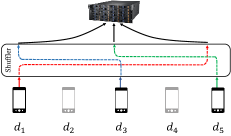
Figure 1: An iteration from the CLDP-SGD Algorithm, where 333 clients are randomly chosen at each iteration. Each client sends the private gradient p(gt(di))subscript𝑝subscript𝑔𝑡subscript𝑑𝑖\mathcal{R}_{p}\left(g_{t}(d_{i})\right) to the shuffler that randomly permutes the gradients before passing them to the server.

In distributed (and federated) learning, a fraction of the data samples are sampled; for example, with random client participation and stochastic gradient descent (SGD), which can be written as

θt+1θtηt1||i(fi(θt)),subscript𝜃𝑡1subscript𝜃𝑡subscript𝜂𝑡1subscript𝑖subscript𝑓𝑖subscript𝜃𝑡\theta_{t+1}\leftarrow\theta_{t}-\eta_{t}\frac{1}{|\mathcal{I}|}\sum_{i\in\mathcal{I}}\mathcal{R}(\nabla f_{i}(\theta_{t})),

where \mathcal{R} is the local randomization mechanism and \mathcal{I} are the indices of the sampled data. This is a subsampled mechanism that enables another privacy amplification opportunity; which, in several cases, is shown to yield a privacy advantage proportional to the subsampling rate; see [KLN+11, Ull17]. The central technical question addressed in this paper is how to analyze the RDP of an arbitrary discrete mechanism for the subsampled shuffle privacy model. This enables us to answer the overall question posed in this paper, which is an achievable privacy-learning performance trade-off point for solving (4) in the shuffled privacy model for distributed learning (see Figure 1). Our contributions are:

  • We analyze the RDP of subsampled mechanisms in the shuffle framework by developing a novel bound applicable to any discrete ϵ0subscriptitalic-ϵ0\epsilon_{0}-LDP mechanism as a function of the RDP order λ𝜆\lambda, subsampling rate γ𝛾\gamma, the LDP parameter ϵ0subscriptitalic-ϵ0\epsilon_{0}, and the number of clients n𝑛n; see Theorem 1. The bound is explicit and amenable to numerics, including all constants.222As emphasized in [WBK19], “in differential privacy, constants matter”. Furthermore, the bounds are valid for generic LDP mechanisms and all parameter regimes.333Some of the best known approximate DP bounds for the shuffle model [BBGN19c, FMT20] are restricted to certain parameter regimes in terms of n,δ,ϵ0𝑛𝛿subscriptitalic-ϵ0n,\delta,\epsilon_{0}, etc. We also provide a lower bound for the RDP in Theorem 2. We prove our upper bound (Theorem 1) using the following novel analysis techniques: First, we reduce the problem of computing the RDP of sub-sampled shuffle mechanisms to the problem of computing ternary |χ|αsuperscript𝜒𝛼|\chi|^{\alpha}-DP [WBK19] of shuffle (non sub-sampled) mechanisms; see Lemma 2. Then we reduce the computation of the ternary |χ|αsuperscript𝜒𝛼|\chi|^{\alpha}-DP of shuffle mechanisms for a generic triple of neighboring datasets to those that have a special structure (see Theorem 5) – this reduction step is one of the core technical results of this paper. Then we bound the ternary |χ|αsuperscript𝜒𝛼|\chi|^{\alpha}-DP of the shuffle mechanisms for triples of neighboring datasets having special structures by bounding the Pearson-Vajda divergence [WBK19] using some concentration properties (see Theorem 6).

  • Using the core technical result in Theorem 1, we analyze privacy-convergence trade-offs of the CLDP-SGD algorithm (see Algorithm 1) for Lipschitz convex functions in Theorem 3. This partially resolves an open question posed in [GDD+21b], to extend their privacy analysis to RDP and significantly strengthening their privacy guarantees.

  • Numerically, we save a factor of 14×14\times in privacy (ϵitalic-ϵ\epsilon) over the best known results for approximate DP for shuffling [FMT20] combined with strong composition [KOV15] for T=105,γ=0.001,n=106formulae-sequence𝑇superscript105formulae-sequence𝛾0.001𝑛superscript106T=10^{5},\gamma=0.001,n=10^{6}. Translating these to privacy-performance operating point in distributed optimization, over the MNIST data set with subscript\ell_{\infty}-norm clipping we numerically show gains: For the same privacy budget of ϵ=1.4italic-ϵ1.4\epsilon=1.4, we get a test performance of 80%percent8080\% whereas using strong composition the test performance of [FMT20] is 70%percent7070\%; furthermore, we achieve 90%percent9090\% accuracy with the total privacy budget ϵ=2.91italic-ϵ2.91\epsilon=2.91, whereas, [FMT20] (with strong composition) achieve the same accuracy with a total privacy budget of ϵ=4.82italic-ϵ4.82\epsilon=4.82. See Section 4 for more results.

Related work:

We give a more complete literature review in Appendix A, and focus here on the works that are closest to the results presented in this paper.

  • Private optimization in the shuffled model: Recently, [EFM+20] and [GDD+21b] have proposed differentially private SGD algorithms for federated learning, where at each iteration, each client applies an LDP mechanism on the gradients with the existence of a secure shuffler between the clients and the central server. However, the privacy analyses in these works developed approximate DP using advanced composition theorems for DP (e.g., [DRV10, KOV15]), which are known to be loose for composition [ACG+16]. To the best of our knowledge, analyzing the private optimization framework using RDP and subsampling in the shuffled model is new to this paper.

  • Subsampled RDP: The works [MTZ19, WBK19, ZW19] have studied the RDP of subsampled mechanisms without shuffling. They demonstrated that this provides a tighter bound on the total privacy loss than the bound that can be obtained using the standard strong composition theorems. The RDP of the shuffled model was very recently studied in [GDD+21a], but without incorporating subsampling, which poses new technical challenges, as directly bounding the RDP of subsampled shuffle mechanisms is non-trivial. We overcome this by reducing our problem of computing RDP to bounding the ternary |χ|αsuperscript𝜒𝛼|\chi|^{\alpha}-DP, and bounding the latter is a core technical contribution of our paper.

Paper organization:

We give preliminaries and problem formulation in Section 2, main results (upper and lower bounds, and privacy-convergence tradeoff) in Section 3, numerical results in Section 4, proof of the upper bound in Section 5, and proof of the ternary DP of the shuffle model in Section 6.

2 Preliminaries and Problem Formulation

We use several privacy definitions throughout this paper. Among these, the local and central differential privacy definitions are standard. The other privacy definitions (Renyi DP and ternary |χ|αsuperscript𝜒𝛼|\chi|^{\alpha}-DP) are relatively less standard and we define them below.

Definition 1 (Local Differential Privacy - LDP [KLN+11]).

For ϵ00subscriptitalic-ϵ00\epsilon_{0}\geq 0, a randomized mechanism :𝒳𝒴:𝒳𝒴\mathcal{R}:\mathcal{X}\to\mathcal{Y} is said to be ϵ0subscriptitalic-ϵ0\epsilon_{0}-local differentially private (in short, ϵ0subscriptitalic-ϵ0\epsilon_{0}-LDP), if for every pair of inputs d,d𝒳𝑑superscript𝑑𝒳d,d^{\prime}\in\mathcal{X}, we have

Pr[(d)𝒮]eϵ0Pr[(d)𝒮],𝒮𝒴.formulae-sequencePr𝑑𝒮superscript𝑒subscriptitalic-ϵ0Prsuperscript𝑑𝒮for-all𝒮𝒴~{}\Pr[\mathcal{R}(d)\in\mathcal{S}]\leq e^{\epsilon_{0}}\Pr[\mathcal{R}(d^{\prime})\in\mathcal{S}],\qquad\forall\mathcal{S}\subseteq\mathcal{Y}. (1)

Let 𝒟={d1,,dn}𝒟subscript𝑑1subscript𝑑𝑛\mathcal{D}=\{d_{1},\ldots,d_{n}\} denote a dataset comprising n𝑛n points from 𝒳𝒳\mathcal{X}. We say that two datasets 𝒟={d1,,dn}𝒟subscript𝑑1subscript𝑑𝑛\mathcal{D}=\{d_{1},\ldots,d_{n}\} and 𝒟={d1,,dn}superscript𝒟superscriptsubscript𝑑1superscriptsubscript𝑑𝑛\mathcal{D}^{\prime}=\{d_{1}^{\prime},\ldots,d_{n}^{\prime}\} are neighboring (and denoted by 𝒟𝒟similar-to𝒟superscript𝒟\mathcal{D}\sim\mathcal{D}^{\prime}) if they differ in one data point, i.e., there exists an i[n]𝑖delimited-[]𝑛i\in[n] such that didisubscript𝑑𝑖subscriptsuperscript𝑑𝑖d_{i}\neq d^{\prime}_{i} and for every j[n],jiformulae-sequence𝑗delimited-[]𝑛𝑗𝑖j\in[n],j\neq i, we have dj=djsubscript𝑑𝑗subscriptsuperscript𝑑𝑗d_{j}=d^{\prime}_{j}.

Definition 2 (Central Differential Privacy - DP [DMNS06, DR14]).

For ϵ,δ0italic-ϵ𝛿0\epsilon,\delta\geq 0, a randomized mechanism :𝒳n𝒴:superscript𝒳𝑛𝒴\mathcal{M}:\mathcal{X}^{n}\to\mathcal{Y} is said to be (ϵ,δ)italic-ϵ𝛿(\epsilon,\delta)-differentially private (in short, (ϵ,δ)italic-ϵ𝛿(\epsilon,\delta)-DP), if for all neighboring datasets 𝒟,𝒟𝒳n𝒟superscript𝒟superscript𝒳𝑛\mathcal{D},\mathcal{D}^{\prime}\in\mathcal{X}^{n} and every subset 𝒮𝒴𝒮𝒴\mathcal{S}\subseteq\mathcal{Y}, we have

Pr[(𝒟)𝒮]eϵ0Pr[(𝒟)𝒮]+δ.Pr𝒟𝒮superscript𝑒subscriptitalic-ϵ0Prsuperscript𝒟𝒮𝛿~{}\Pr\left[\mathcal{M}(\mathcal{D})\in\mathcal{S}\right]\leq e^{\epsilon_{0}}\Pr\left[\mathcal{M}(\mathcal{D}^{\prime})\in\mathcal{S}\right]+\delta. (2)
Definition 3 ((λ,ϵ)𝜆italic-ϵ(\lambda,\epsilon)-RDP (Renyi Differential Privacy) [Mir17]).

A randomized mechanism :𝒳n𝒴:superscript𝒳𝑛𝒴\mathcal{M}:\mathcal{X}^{n}\to\mathcal{Y} is said to have ϵitalic-ϵ\epsilon-Renyi differential privacy of order λ(1,)𝜆1\lambda\in(1,\infty) (in short, (λ,ϵ(λ))𝜆italic-ϵ𝜆(\lambda,\epsilon(\lambda))-RDP), if for any neighboring datasets 𝒟𝒟\mathcal{D}, 𝒟𝒳nsuperscript𝒟superscript𝒳𝑛\mathcal{D}^{\prime}\in\mathcal{X}^{n}, the Renyi divergence of order λ𝜆\lambda between (𝒟)𝒟\mathcal{M}(\mathcal{D}) and (𝒟)superscript𝒟\mathcal{M}(\mathcal{D}^{\prime}) is upper-bounded by ϵ(λ)italic-ϵ𝜆\epsilon(\lambda), i.e.,

Dλ((𝒟)||(𝒟))=1λ1log(𝔼θ(𝒟)[((𝒟)(θ)(𝒟)(θ))λ])ϵ(λ),D_{\lambda}(\mathcal{M}(\mathcal{D})||\mathcal{M}(\mathcal{D}^{\prime}))=\frac{1}{\lambda-1}\log\left(\mathbb{E}_{\theta\sim\mathcal{M}(\mathcal{D}^{\prime})}\left[\left(\frac{\mathcal{M}(\mathcal{D})(\theta)}{\mathcal{M}(\mathcal{D}^{\prime})(\theta)}\right)^{\lambda}\right]\right)\leq\epsilon(\lambda), (3)

where (𝒟)(θ)𝒟𝜃\mathcal{M}(\mathcal{D})(\theta) denotes the probability that \mathcal{M} on input 𝒟𝒟\mathcal{D} generates the output θ𝜃\theta.

Definition 4 (ζ𝜁\zeta-Ternary |χ|αsuperscript𝜒𝛼|\chi|^{\alpha}-differential privacy [WBK19]).

A randomized mechanism :𝒳n𝒴:superscript𝒳𝑛𝒴\mathcal{M}:\mathcal{X}^{n}\to\mathcal{Y} is said to have ζ𝜁\zeta-ternary-|χ|αsuperscript𝜒𝛼|\chi|^{\alpha}-DP, if for any triple of mutually adjacent datasets 𝒟,𝒟,𝒟′′𝒳n𝒟superscript𝒟superscript𝒟′′superscript𝒳𝑛\mathcal{D},\mathcal{D}^{\prime},\mathcal{D}^{\prime\prime}\in\mathcal{X}^{n} (i.e., they mutually differ in the same location), the ternary-|χ|αsuperscript𝜒𝛼|\chi|^{\alpha} divergence of (𝒟),(𝒟),(𝒟)𝒟superscript𝒟superscript𝒟\mathcal{M}(\mathcal{D}),\mathcal{M}(\mathcal{D}^{\prime}),\mathcal{M}(\mathcal{D}^{\prime}) is upper-bounded by (ζ(α))αsuperscript𝜁𝛼𝛼(\zeta(\alpha))^{\alpha} for all α1𝛼1\alpha\geq 1 (where ζ𝜁\zeta is a function from +superscript\mathbb{R}^{+} to +superscript\mathbb{R}^{+}), i.e.,

D|χ|α((𝒟),(𝒟)||(𝒟′′)):=𝔼(𝒟′′)[|(𝒟)(𝒟)(𝒟′′)|α](ζ(α))α.D_{|\chi|^{\alpha}}\left(\mathcal{M}(\mathcal{D}),\mathcal{M}(\mathcal{D}^{\prime})||\mathcal{M}(\mathcal{D}^{\prime\prime})\right):=\mathbb{E}_{\mathcal{M}(\mathcal{D}^{\prime\prime})}\left[\left|\frac{\mathcal{M}(\mathcal{D})-\mathcal{M}(\mathcal{D}^{\prime})}{\mathcal{M}(\mathcal{D}^{\prime\prime})}\right|^{\alpha}\right]\leq\left(\zeta(\alpha)\right)^{\alpha}.

The ternary |χ|αsuperscript𝜒𝛼|\chi|^{\alpha}-DP was proposed in [WBK19] to characterize the RDP of the sub-sampled mechanism without shuffling. In this work, we analyze the ternary |χ|αsuperscript𝜒𝛼|\chi|^{\alpha}-DP of the shuffled mechanism to bound the RDP of the sub-sampled shuffle model.

We can use the following result for converting the RDP guarantees of a mechanism to its central DP guarantees. To the best of our knowledge, this result gives the best conversion.

Lemma 1 (From RDP to DP [CKS20, BBG+20]).

Suppose for any λ>1𝜆1\lambda>1, a mechanism \mathcal{M} is (λ,ϵ(λ))𝜆italic-ϵ𝜆\left(\lambda,\epsilon\left(\lambda\right)\right)-RDP. Then, the mechanism \mathcal{M} is (ϵ,δ)italic-ϵ𝛿\left(\epsilon,\delta\right)-DP, where δ>0𝛿0\delta>0 is arbitrary and ϵitalic-ϵ\epsilon is given by

ϵ=minλ(ϵ(λ)+log(1/δ)+(λ1)log(11/λ)log(λ)λ1).italic-ϵsubscript𝜆italic-ϵ𝜆1𝛿𝜆111𝜆𝜆𝜆1\epsilon=\min_{\lambda}\left(\epsilon\left(\lambda\right)+\frac{\log\left(1/\delta\right)+\left(\lambda-1\right)\log\left(1-1/\lambda\right)-\log\left(\lambda\right)}{\lambda-1}\right).

2.1 Problem formulation

We consider a distributed private learning setup comprising a set of n𝑛n clients, where the i𝑖ith client has a data point disubscript𝑑𝑖d_{i} drawn from a universe 𝒳𝒳\mathcal{X} for i[n]𝑖delimited-[]𝑛i\in\left[n\right]; see also Figure 1. Let 𝒟=(d1,,dn)𝒟subscript𝑑1subscript𝑑𝑛\mathcal{D}=\left(d_{1},\ldots,d_{n}\right) denote the entire training dataset. The clients are connected to an untrusted server in order to solve the following empirical risk minimization (ERM) problem

minθ𝒞(F(θ,𝒟):=1ni=1nf(θ,di)),subscript𝜃𝒞assign𝐹𝜃𝒟1𝑛superscriptsubscript𝑖1𝑛𝑓𝜃subscript𝑑𝑖\min_{\theta\in\mathcal{C}}\Big{(}F(\theta,\mathcal{D}):=\frac{1}{n}\sum_{i=1}^{n}f(\theta,d_{i})\Big{)}, (4)

where 𝒞d𝒞superscript𝑑\mathcal{C}\subset\mathbb{R}^{d} is a closed convex set, and f:𝒞×𝒟:𝑓𝒞𝒟f:\mathcal{C}\times\mathcal{D}\to\mathbb{R} is the loss function. Our goal is to construct a global learning model θ𝜃\theta via stochastic gradient descent (SGD) while preserving privacy of individual data points in the training dataset 𝒟𝒟\mathcal{D} by providing strong DP guarantees.

Algorithm 1 𝒜cldpsubscript𝒜cldp\mathcal{A}_{\text{cldp}}: CLDP-SGD
1:Input: Datasets 𝒟=(d1,,dn)𝒟subscript𝑑1subscript𝑑𝑛\mathcal{D}=\left(d_{1},\ldots,d_{n}\right), LDP privacy parameter ϵ0subscriptitalic-ϵ0\epsilon_{0}, gradient norm bound C𝐶C, and learning rate schedule {ηt}subscript𝜂𝑡\{\eta_{t}\}.
2:Initialize: θ0𝒞subscript𝜃0𝒞\theta_{0}\in\mathcal{C}
3:for t[T]𝑡delimited-[]𝑇t\in\left[T\right] do
4:     Client sampling: A random set 𝒰tsubscript𝒰𝑡\mathcal{U}_{t} of k𝑘k clients is chosen.
5:     for clients i𝒰t𝑖subscript𝒰𝑡i\in\mathcal{U}_{t} do
6:         Compute gradient: 𝐠t(di)θtf(θt,di)subscript𝐠𝑡subscript𝑑𝑖subscriptsubscript𝜃𝑡𝑓subscript𝜃𝑡subscript𝑑𝑖\mathbf{g}_{t}\left(d_{i}\right)\leftarrow\nabla_{\theta_{t}}f\left(\theta_{t},d_{i}\right)
7:         Clip gradient: 𝐠~t(di)𝐠t(di)/max{1,𝐠t(di)pC}subscript~𝐠𝑡subscript𝑑𝑖subscript𝐠𝑡subscript𝑑𝑖1subscriptnormsubscript𝐠𝑡subscript𝑑𝑖𝑝𝐶\tilde{\mathbf{g}}_{t}\left(d_{i}\right)\leftarrow\mathbf{g}_{t}\left(d_{i}\right)/\max\left\{1,\frac{\|\mathbf{g}_{t}\left(d_{i}\right)\|_{p}}{C}\right\}
8:         Client i𝑖i sends p(𝐠~t(di))subscript𝑝subscript~𝐠𝑡subscript𝑑𝑖\mathcal{R}_{p}\left(\tilde{\mathbf{g}}_{t}\left(d_{i}\right)\right) to the shuffler.      
9:     Shuffling: The shuffler sends random permutation of {p(𝐠~t(di)):i𝒰t}conditional-setsubscript𝑝subscript~𝐠𝑡subscript𝑑𝑖𝑖subscript𝒰𝑡\{\mathcal{R}_{p}\left(\tilde{\mathbf{g}}_{t}\left(d_{i}\right)\right):i\in\mathcal{U}_{t}\} to the server.
10:     Aggregate: 𝐠¯t1ki𝒰tp(𝐠~t(di))subscript¯𝐠𝑡1𝑘subscript𝑖subscript𝒰𝑡subscript𝑝subscript~𝐠𝑡subscript𝑑𝑖\overline{\mathbf{g}}_{t}\leftarrow\frac{1}{k}\sum_{i\in\mathcal{U}_{t}}\mathcal{R}_{p}\left(\tilde{\mathbf{g}}_{t}\left(d_{i}\right)\right)
11:     Descent Step: θt+1𝒞(θtηt𝐠¯t)subscript𝜃𝑡1subscriptproduct𝒞subscript𝜃𝑡subscript𝜂𝑡subscript¯𝐠𝑡\theta_{t+1}\leftarrow\prod_{\mathcal{C}}\left(\theta_{t}-\eta_{t}\overline{\mathbf{g}}_{t}\right), where 𝒞subscriptproduct𝒞\prod_{\mathcal{C}} is the projection operator onto the set 𝒞𝒞\mathcal{C}.
12:
13:Output: The model θTsubscript𝜃𝑇\theta_{T} and the privacy parameters ϵitalic-ϵ\epsilon, δ𝛿\delta.

We revisit the CLDP-SGD algorithm presented in [GDD+21b] and described in Algorithm 1 to solve the ERM (4). In each step of CLDP-SGD, we choose uniformly at random a set 𝒰tsubscript𝒰𝑡\mathcal{U}_{t} of kn𝑘𝑛k\leq n clients out of n𝑛n clients. Each client i𝒰t𝑖subscript𝒰𝑡i\in\mathcal{U}_{t} computes and clips the psubscript𝑝\ell_{p}-norm of the gradient θtf(θt,di)subscriptsubscript𝜃𝑡𝑓subscript𝜃𝑡subscript𝑑𝑖\nabla_{\theta_{t}}f\left(\theta_{t},d_{i}\right) to apply the LDP mechanism psubscript𝑝\mathcal{R}_{p}, where p:pd{0,1}b:subscript𝑝superscriptsubscript𝑝𝑑superscript01𝑏\mathcal{R}_{p}:\mathcal{B}_{p}^{d}\to\{0,1\}^{b} is an ϵ0subscriptitalic-ϵ0\epsilon_{0}-LDP mechanism when inputs come from the psubscript𝑝\ell_{p}-norm ball pd={𝒙d:𝒙p1}superscriptsubscript𝑝𝑑conditional-set𝒙superscript𝑑subscriptnorm𝒙𝑝1\mathcal{B}_{p}^{d}=\{\boldsymbol{x}\in\mathbb{R}^{d}:\|\boldsymbol{x}\|_{p}\leq 1\}, where 𝒙p=(i=1d|xi|p)1/psubscriptnorm𝒙𝑝superscriptsuperscriptsubscript𝑖1𝑑superscriptsubscript𝑥𝑖𝑝1𝑝\|\boldsymbol{x}\|_{p}=\left(\sum_{i=1}^{d}|x_{i}|^{p}\right)^{1/p} denotes the psubscript𝑝\ell_{p}-norm of the vector 𝒙d𝒙superscript𝑑\boldsymbol{x}\in\mathbb{R}^{d}. In [GDD+21b], we proposed different ϵ0subscriptitalic-ϵ0\epsilon_{0}-LDP mechanisms for general psubscript𝑝\ell_{p}-norm balls. After that, the shuffler randomly permutes the received k𝑘k gradients {p(𝐠~t(di))}i𝒰tsubscriptsubscript𝑝subscript~𝐠𝑡subscript𝑑𝑖𝑖subscript𝒰𝑡\{\mathcal{R}_{p}\left(\tilde{\mathbf{g}}_{t}\left(d_{i}\right)\right)\}_{i\in\mathcal{U}_{t}} and sends them to the server. Finally, the server takes the average of the received gradients and updates the parameter vector. Our main contribution in this work is to present a stronger privacy analysis of the CLDP-SGD algorithm by characterizing the RDP of the sub-sampled shuffle model.

3 Main Results

In this section, we present our main results. First, we characterize the RDP of the subsampled shuffle mechanism by presenting an upper bound in Theorem 1 and a lower bound in Theorem 2. We then present the privacy-convergence trade-offs of the CLDP-SGD Algorithm in Theorem 3.

Consider an arbitrary ϵ0subscriptitalic-ϵ0\epsilon_{0}-LDP mechanism \mathcal{R}, whose range is a discrete set [B]={1,,B}delimited-[]𝐵1𝐵\left[B\right]=\left\{1,\ldots,B\right\} for some B:={1,2,3,}𝐵assign123B\in\mathbb{N}:=\{1,2,3,\ldots\}. Here, [B]delimited-[]𝐵[B] could be the whole of \mathbb{N}. Let (𝒟)𝒟\mathcal{M}(\mathcal{D}) be a subsampled shuffle mechanism defined as follows: First subsample kn𝑘𝑛k\leq n clients of the n𝑛n clients (without replacement), where γ=kn𝛾𝑘𝑛\gamma=\frac{k}{n} denotes the sampling parameter. Each client i𝑖i out of the k𝑘k selected clients applies \mathcal{R} on disubscript𝑑𝑖d_{i} and sends (di)subscript𝑑𝑖\mathcal{R}(d_{i}) to the shuffler,444With a slight abuse of notation, in this paper we write (di)subscript𝑑𝑖\mathcal{R}(d_{i}) to denote that \mathcal{R} takes as its input the gradient computed on disubscript𝑑𝑖d_{i} using the current parameter vector. who randomly permutes the received k𝑘k inputs and outputs the result. To formalize this, let k:𝒴k𝒴k:subscript𝑘superscript𝒴𝑘superscript𝒴𝑘\mathcal{H}_{k}:\mathcal{Y}^{k}\to\mathcal{Y}^{k} denote the shuffling operation that takes k𝑘k inputs and outputs their uniformly random permutation. Let sampkn:𝒳n𝒳k:superscriptsubscriptsamp𝑘𝑛superscript𝒳𝑛superscript𝒳𝑘\mathrm{samp}_{k}^{n}:\mathcal{X}^{n}\to\mathcal{X}^{k} denote the sampling operation for choosing a random subset of k𝑘k elements from a set of n𝑛n elements. We define the subsampled-shuffle mechanism as

(𝒟):=ksampkn((d1),,(dn)).assign𝒟subscript𝑘superscriptsubscriptsamp𝑘𝑛subscript𝑑1subscript𝑑𝑛\mathcal{M}\left(\mathcal{D}\right):=\mathcal{H}_{k}\circ\mathrm{samp}_{k}^{n}\left(\mathcal{R}\left(d_{1}\right),\ldots,\mathcal{R}\left(d_{n}\right)\right). (5)

Observe that each iteration of Algorithm 1 can be represented as an output of the subsampled shuffle mechanism \mathcal{M}. Thus, to analyze the privacy of Algorithm 1, it is sufficient to analyze the privacy of a sequence of identical T𝑇T subsampled shuffle mechanisms, and then apply composition theorems.

Histogram notation.

It will be useful to define the following notation. Since the output of ksubscript𝑘\mathcal{H}_{k} is a random permutation of the k𝑘k outputs of \mathcal{R} (subsampling is not important here), the server cannot associate the k𝑘k messages to the clients; and the only information it can use from the messages is the histogram, i.e., the number of messages that give any particular output in [B]delimited-[]𝐵[B]. We define a set 𝒜Bksuperscriptsubscript𝒜𝐵𝑘\mathcal{A}_{B}^{k} as

𝒜Bk={𝒉=(h1,,hB):j=1Bhj=k},superscriptsubscript𝒜𝐵𝑘conditional-set𝒉subscript1subscript𝐵superscriptsubscript𝑗1𝐵subscript𝑗𝑘\mathcal{A}_{B}^{k}=\bigg{\{}\boldsymbol{h}=\left(h_{1},\ldots,h_{B}\right):\sum_{j=1}^{B}h_{j}=k\bigg{\}}, (6)

to denote the set of all possible histograms of the output of the shuffler with k𝑘k inputs. Therefore, we can assume, without loss of generality (w.l.o.g.), that the output of \mathcal{M} is a distribution over 𝒜Bksuperscriptsubscript𝒜𝐵𝑘\mathcal{A}_{B}^{k}.

Our main results for the RDP of the subsampled shuffled mechanism (defined in (5)) are given below. Our first result provides an upper bound (stated in Theorem 1 and proved in Section 5) and the second result provides a lower bound (stated in Theorem 2 and proved in Section 7).

Theorem 1 (Upper Bound).

For any n𝑛n\in\mathbb{N}, kn𝑘𝑛k\leq n, ϵ00subscriptitalic-ϵ00\epsilon_{0}\geq 0, and any integer λ2𝜆2\lambda\geq 2, the RDP of the subsampled shuffle mechanism \mathcal{M} (defined in (5)) is upper-bounded by

ϵ(λ)1λ1log(1+4(λ2)γ2(eϵ01)2k¯eϵ0+j=3λ(λj)γjjΓ(j/2)(2(e2ϵ01)2k¯e2ϵ0)j/2+Υ),italic-ϵ𝜆1𝜆114binomial𝜆2superscript𝛾2superscriptsuperscript𝑒subscriptitalic-ϵ012¯𝑘superscript𝑒subscriptitalic-ϵ0superscriptsubscript𝑗3𝜆binomial𝜆𝑗superscript𝛾𝑗𝑗Γ𝑗2superscript2superscriptsuperscript𝑒2subscriptitalic-ϵ012¯𝑘superscript𝑒2subscriptitalic-ϵ0𝑗2Υ\epsilon(\lambda)\leq\frac{1}{\lambda-1}\log\left(1+4\binom{\lambda}{2}\gamma^{2}\frac{\left(e^{\epsilon_{0}}-1\right)^{2}}{\overline{k}e^{\epsilon_{0}}}+\sum_{j=3}^{\lambda}\binom{\lambda}{j}\gamma^{j}j\Gamma\left(j/2\right)\left(\frac{2\left(e^{2\epsilon_{0}}-1\right)^{2}}{\overline{k}e^{2\epsilon_{0}}}\right)^{j/2}+\Upsilon\right),

where k¯=k12eϵ0+1¯𝑘𝑘12superscript𝑒subscriptitalic-ϵ01\overline{k}=\lfloor\frac{k-1}{2e^{\epsilon_{0}}}\rfloor+1, γ=kn𝛾𝑘𝑛\gamma=\frac{k}{n}, and Γ(z)=0xz1ex𝑑xΓ𝑧superscriptsubscript0superscript𝑥𝑧1superscript𝑒𝑥differential-d𝑥\Gamma\left(z\right)=\int_{0}^{\infty}x^{z-1}e^{-x}dx is the Gamma function. The term ΥΥ\Upsilon is given by Υ=((1+γe2ϵ01eϵ0)λ1λγe2ϵ01eϵ0)ek18eϵ0Υsuperscript1𝛾superscript𝑒2subscriptitalic-ϵ01superscript𝑒subscriptitalic-ϵ0𝜆1𝜆𝛾superscript𝑒2subscriptitalic-ϵ01superscript𝑒subscriptitalic-ϵ0superscript𝑒𝑘18superscript𝑒subscriptitalic-ϵ0\Upsilon=\left(\left(1+\gamma\frac{e^{2\epsilon_{0}}-1}{e^{\epsilon_{0}}}\right)^{\lambda}-1-\lambda\gamma\frac{e^{2\epsilon_{0}}-1}{e^{\epsilon_{0}}}\right)e^{-\frac{k-1}{8e^{\epsilon_{0}}}}.

Theorem 2 (Lower Bound).

For any n𝑛n\in\mathbb{N}, kn𝑘𝑛k\leq n, ϵ00subscriptitalic-ϵ00\epsilon_{0}\geq 0, and any integer λ2𝜆2\lambda\geq 2, the RDP of the subsampled shuffle mechanism \mathcal{M} (defined in (5)) is lower-bounded by

ϵ(λ)1λ1log(1+(λ2)γ2(eϵ01)2keϵ0+j=3λ(λj)γj((e2ϵ01)keϵ0)j𝔼(mkeϵ0+1)j),italic-ϵ𝜆1𝜆11binomial𝜆2superscript𝛾2superscriptsuperscript𝑒subscriptitalic-ϵ012𝑘superscript𝑒subscriptitalic-ϵ0superscriptsubscript𝑗3𝜆binomial𝜆𝑗superscript𝛾𝑗superscriptsuperscript𝑒2subscriptitalic-ϵ01𝑘superscript𝑒subscriptitalic-ϵ0𝑗𝔼superscript𝑚𝑘superscript𝑒subscriptitalic-ϵ01𝑗\epsilon\left(\lambda\right)\geq\frac{1}{\lambda-1}\log\left(1+\binom{\lambda}{2}\gamma^{2}\frac{\left(e^{\epsilon_{0}}-1\right)^{2}}{ke^{\epsilon_{0}}}+\sum_{j=3}^{\lambda}\binom{\lambda}{j}\gamma^{j}\left(\frac{\left(e^{2\epsilon_{0}}-1\right)}{ke^{\epsilon_{0}}}\right)^{j}\mathbb{E}\left(m-\frac{k}{e^{\epsilon_{0}}+1}\right)^{j}\right),

where expectation is taken w.r.t. the binomial r.v. mBin(k,p)similar-to𝑚Bin𝑘𝑝m\sim\text{Bin}\left(k,p\right) with parameter p=1eϵ0+1𝑝1superscript𝑒subscriptitalic-ϵ01p=\frac{1}{e^{\epsilon_{0}}+1}.

The CLDP-SGD algorithm and its privacy-convergence trade-offs (stated in Theorem 3 below) are given for a general local randomizer psubscript𝑝\mathcal{R}_{p} (whose inputs comes from an psubscript𝑝\ell_{p}-ball for any p[1,]𝑝1p\in[1,\infty]) that satisfies the following conditions: (i) The randomized mechanism psubscript𝑝\mathcal{R}_{p} is an ϵ0subscriptitalic-ϵ0\epsilon_{0}-LDP mechanism. (ii) The randomized mechanism psubscript𝑝\mathcal{R}_{p} is unbiased, i.e., 𝔼[p(𝐱)|𝐱]=𝐱𝔼delimited-[]conditionalsubscript𝑝𝐱𝐱𝐱\mathbb{E}\left[\mathcal{R}_{p}\left(\mathbf{x}\right)|\mathbf{x}\right]=\mathbf{x} for all 𝐱p(a)𝐱subscript𝑝𝑎\mathbf{x}\in\mathcal{B}_{p}(a), where a𝑎a is the radius of the ball psubscript𝑝\mathcal{B}_{p}. (iii) The output of the randomized mechanism psubscript𝑝\mathcal{R}_{p} can be represented using B+𝐵superscriptB\in\mathbb{N}^{+} bits. (iv) The randomized psubscript𝑝\mathcal{R}_{p} has a bounded variance: sup𝐱p(a)𝔼p(𝐱)𝐱22Gp2(a)subscriptsupremum𝐱subscript𝑝𝑎𝔼superscriptsubscriptnormsubscript𝑝𝐱𝐱22superscriptsubscript𝐺𝑝2𝑎\sup_{\mathbf{x}\in\mathcal{B}_{p}(a)}\mathbb{E}\|\mathcal{R}_{p}\left(\mathbf{x}\right)-\mathbf{x}\|_{2}^{2}\leq G_{p}^{2}(a), where Gp2superscriptsubscript𝐺𝑝2G_{p}^{2} is a function from +superscript\mathbb{R}^{+} to +superscript\mathbb{R}^{+}.

[GDD+21b] proposed unbiased ϵ0subscriptitalic-ϵ0\epsilon_{0}-LDP mechanisms psubscript𝑝\mathcal{R}_{p} for several values of norms p[1,]𝑝1p\in[1,\infty] that require b=𝒪(log(d))𝑏𝒪𝑑b=\mathcal{O}\left(\log\left(d\right)\right) bits of communication and satisfy the above conditions. In this paper, achieving communication efficiency is not our goal (though we also achieve that since the ϵ0subscriptitalic-ϵ0\epsilon_{0}-LDP mechanism psubscript𝑝\mathcal{R}_{p} that we use takes values in a discrete set), as our main focus is on analyzing the RDP of the subsampled shuffle mechanism. If we use the ϵ0subscriptitalic-ϵ0\epsilon_{0}-LDP mechanism psubscript𝑝\mathcal{R}_{p} from [GDD+21b], we would also get similar gains in communication as were obtained in [GDD+21b].

The privacy-convergence trade-off of our algorithm 𝒜cldpsubscript𝒜cldp\mathcal{A}_{\text{cldp}} is given below.

Theorem 3 (Privacy-Convergence tradeoffs).

Let the set 𝒞𝒞\mathcal{C} be convex with diameter D𝐷D and the function f(θ;.):𝒞×𝒟f\left(\theta;.\right):\mathcal{C}\times\mathcal{D}\to\mathbb{R} be convex and L𝐿L-Lipschitz continuous with respect to the gsubscript𝑔\ell_{g}-norm, which is the dual of the psubscript𝑝\ell_{p}-norm. Let θ=argminθ𝒞F(θ)superscript𝜃subscript𝜃𝒞𝐹𝜃\theta^{*}=\arg\min_{\theta\in\mathcal{C}}F\left(\theta\right) denote the minimizer of the problem (4). For γ=kn𝛾𝑘𝑛\gamma=\frac{k}{n}, if we run Algorithm 𝒜cldpsubscript𝒜cldp\mathcal{A}_{\emph{cldp}} over T𝑇T iterations, then we have

  1. 1.

    Privacy: 𝒜cldpsubscript𝒜cldp\mathcal{A}_{\emph{cldp}} is (ϵ,δ)italic-ϵ𝛿\left(\epsilon,\delta\right)-DP, where δ>0𝛿0\delta>0 is arbitrary and ϵitalic-ϵ\epsilon is given by

    ϵ=minλ(Tϵ(λ)+log(1/δ)+(λ1)log(11/λ)log(λ)λ1),italic-ϵsubscript𝜆𝑇italic-ϵ𝜆1𝛿𝜆111𝜆𝜆𝜆1\epsilon=\min_{\lambda}\left(T\epsilon\left(\lambda\right)+\frac{\log\left(1/\delta\right)+\left(\lambda-1\right)\log\left(1-1/\lambda\right)-\log\left(\lambda\right)}{\lambda-1}\right), (7)

    where ϵ(λ)italic-ϵ𝜆\epsilon\left(\lambda\right) is the RDP of the subsampled shuffle mechanism given in Theorem 1.

  2. 2.

    Convergence: If we run 𝒜cldpsubscript𝒜cldp\mathcal{A}_{\emph{cldp}} with ηt=DGtsubscript𝜂𝑡𝐷𝐺𝑡\eta_{t}=\frac{D}{G\sqrt{t}}, where G2=max{d12p,1}L2+Gp2(L)γnsuperscript𝐺2superscript𝑑12𝑝1superscript𝐿2superscriptsubscript𝐺𝑝2𝐿𝛾𝑛G^{2}=\max\{d^{1-\frac{2}{p}},1\}L^{2}+\frac{G_{p}^{2}(L)}{\gamma n}, we get

    𝔼[F(θT)]F(θ)𝒪(DGlog(T)T).𝔼delimited-[]𝐹subscript𝜃𝑇𝐹superscript𝜃𝒪𝐷𝐺𝑇𝑇\displaystyle\mathbb{E}\left[F\left(\theta_{T}\right)\right]-F\left(\theta^{*}\right)\leq\mathcal{O}\left(\frac{DG\log(T)}{\sqrt{T}}\right).

The proof outline of Theorem 3 is as follows: Note that 𝒜cldpsubscript𝒜cldp\mathcal{A}_{\text{cldp}} is an iterative algorithm, where in each iteration we use the subsampled shuffle mechanism as defined in (5), for which we have computed the RDP guarantees in Theorem 1. Now, for the privacy analysis of 𝒜cldpsubscript𝒜cldp\mathcal{A}_{\text{cldp}}, we use the adaptive composition theorem from [Mir17, Proposition 1] and then use the RDP to DP conversion given in Lemma 1. For the convergence analysis, we use a standard non-private SGD convergence result and compute the required parameters for that. See Section 8 for a complete proof of Theorem 3.

Remark 1.

Note that our convergence bound is affected by the variance of the ϵ0subscriptitalic-ϵ0\epsilon_{0}-LDP mechanism psubscript𝑝\mathcal{R}_{p}. For example, when f𝑓f is L𝐿L-Lipschitz continuous w.r.t. the 2subscript2\ell_{2}-norm, we can use the LDP mechanism 2subscript2\mathcal{R}_{2} proposed in [BDF+18] that has variance G22(L)=14L2d(eϵ0+1eϵ01)2superscriptsubscript𝐺22𝐿14superscript𝐿2𝑑superscriptsuperscript𝑒subscriptitalic-ϵ01superscript𝑒subscriptitalic-ϵ012G_{2}^{2}(L)=14L^{2}d\big{(}\frac{e^{\epsilon_{0}}+1}{e^{\epsilon_{0}}-1}\big{)}^{2}; and when f𝑓f is L𝐿L-Lipschitz continuous w.r.t. the 1subscript1\ell_{1}-norm or subscript\ell_{\infty}-norm, we can use the LDP mechanisms subscript\mathcal{R}_{\infty} or 1subscript1\mathcal{R}_{1}, respectively, proposed in [GDD+21b] that have variances G2(L)=L2d2(eϵ0+1eϵ01)2superscriptsubscript𝐺2𝐿superscript𝐿2superscript𝑑2superscriptsuperscript𝑒subscriptitalic-ϵ01superscript𝑒subscriptitalic-ϵ012G_{\infty}^{2}(L)=L^{2}d^{2}\big{(}\frac{e^{\epsilon_{0}}+1}{e^{\epsilon_{0}}-1}\big{)}^{2} and G12(L)=L2d(eϵ0+1eϵ01)2superscriptsubscript𝐺12𝐿superscript𝐿2𝑑superscriptsuperscript𝑒subscriptitalic-ϵ01superscript𝑒subscriptitalic-ϵ012G_{1}^{2}(L)=L^{2}d\big{(}\frac{e^{\epsilon_{0}}+1}{e^{\epsilon_{0}}-1}\big{)}^{2}, respectively. By plugging these variances Gp2(L)superscriptsubscript𝐺𝑝2𝐿G_{p}^{2}(L) (for p=1,2,𝑝12p=1,2,\infty) into Theorem 3, we get the convergence rate of the L𝐿L-Lipschitz continuous loss function w.r.t. the psubscript𝑝\ell_{p}-norm (for p=,2,1𝑝21p=\infty,2,1).

Remark 2.

The privacy parameter in (7) is not in a closed form expression and could be obtained by solving an optimization problem. However, we numerically compute it for several interesting regimes of parameters in our numerical experiments; see Section 4 for more details.

4 Numerical Results

In this section, we present numerical experiments to show the performance of our bounds on RDP of the subsampled shuffle mechanism and its usage for getting approximate DP of Algorithm 1 for training machine learning models.

Refer to caption
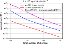
(a) Approx. DP as a function of T𝑇T for ϵ0=2subscriptitalic-ϵ02\epsilon_{0}=2, γ=0.001𝛾0.001\gamma=0.001, n=106𝑛superscript106n=10^{6}
Refer to caption
(b) Approx. DP as a function of T𝑇T for ϵ0=1subscriptitalic-ϵ01\epsilon_{0}=1, γ=0.001𝛾0.001\gamma=0.001, n=107𝑛superscript107n=10^{7}
Refer to caption
(c) Approx. DP as a function of n𝑛n for ϵ0=2subscriptitalic-ϵ02\epsilon_{0}=2, γn=103𝛾𝑛superscript103\gamma n=10^{3}, T=105𝑇superscript105T=10^{5}
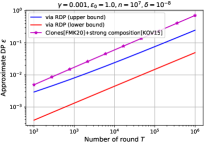
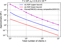
Figure 2: Comparison of several bounds on the Approximate (ϵ,δ)italic-ϵ𝛿\left(\epsilon,\delta\right)-DP for composition of a sequence of subsampled shuffle mechanisms for δ=108𝛿superscript108\delta=10^{-8}: (i) Approximate DP obtained from our upper bound on the RDP in Theorem 1 (blue); (ii) Approximate DP obtained from our lower bound on the RDP in Theorem 2 (red); and (iii) Applying the strong composition theorem [KOV15] after getting the Approximate DP of the shuffled model given in [FMT20] with subsampling [Ull17] (magenta).
Refer to caption
(a) Approx. DP as a function of T𝑇T for ϵ0=1subscriptitalic-ϵ01\epsilon_{0}=1, γ=0.001𝛾0.001\gamma=0.001, n=106𝑛superscript106n=10^{6}
Refer to caption
(b) Approx. DP as a function of T𝑇T for ϵ0=1subscriptitalic-ϵ01\epsilon_{0}=1, γ=0.001𝛾0.001\gamma=0.001, n=107𝑛superscript107n=10^{7}
Refer to caption
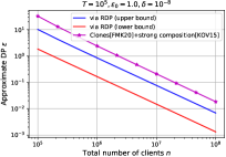
(c) Approx. DP as a function of n𝑛n for ϵ0=1subscriptitalic-ϵ01\epsilon_{0}=1, γn=104𝛾𝑛superscript104\gamma n=10^{4}, T=105𝑇superscript105T=10^{5}
Figure 3: Comparison of our bound on the Approximate (ϵ,δ)italic-ϵ𝛿\left(\epsilon,\delta\right)-DP (blue) for composition of a sequence of subsampled shuffle mechanisms for δ=108𝛿superscript108\delta=10^{-8} with applying the strong composition theorem [KOV15] after getting the Approximate DP of the shuffled model given in [FMT20] with subsampling [Ull17] (magenta).
Refer to caption
(a) Approx. DP as a function of T𝑇T for ϵ0=3subscriptitalic-ϵ03\epsilon_{0}=3, γ=0.001𝛾0.001\gamma=0.001, n=106𝑛superscript106n=10^{6}
Refer to caption
(b) Approx. DP as a function of T𝑇T for ϵ0=3subscriptitalic-ϵ03\epsilon_{0}=3, γ=0.0001𝛾0.0001\gamma=0.0001, n=107𝑛superscript107n=10^{7}
Refer to caption
(c) Approx. DP as a function of n𝑛n for ϵ0=3subscriptitalic-ϵ03\epsilon_{0}=3, γn=103𝛾𝑛superscript103\gamma n=10^{3}, T=105𝑇superscript105T=10^{5}
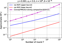
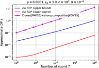
Figure 4: Comparison of several bounds on the Approximate (ϵ,δ)italic-ϵ𝛿\left(\epsilon,\delta\right)-DP for composition of a sequence of subsampled shuffle mechanisms for δ=108𝛿superscript108\delta=10^{-8}: (i) Approximate DP obtained from our upper bound on the RDP in Theorem 1 (blue); (ii) Approximate DP obtained from our lower bound on the RDP in Theorem 2 (red); and (iv) Applying the strong composition theorem [KOV15] after getting the Approximate DP of the shuffled model given in [FMT20] with subsampling [Ull17] (magenta).

Composition of a sequence of subsampled shuffle models:

In Figures 2 and 3, we plot several bounds on the approximate (ϵ,δ)italic-ϵ𝛿\left(\epsilon,\delta\right)-DP for a composition of T𝑇T mechanisms (1,,T)subscript1subscript𝑇\left(\mathcal{M}_{1},\ldots,\mathcal{M}_{T}\right), where tsubscript𝑡\mathcal{M}_{t} is a subsampled shuffle mechanism for t[T]𝑡delimited-[]𝑇t\in\left[T\right]. In all our experiments reported in Figures 2 and 3, we fix δ=108𝛿superscript108\delta=10^{-8}. In Figures 2(c) and 3(c), we fix the number of subsampled clients per iteration to be k=γn=103𝑘𝛾𝑛superscript103k=\gamma n=10^{3} and k=104𝑘superscript104k=10^{4}, respectively. Hence, the subsampling parameter γ𝛾\gamma varies with n𝑛n. We observe that our new bound on the RDP of the subsampled shuffle mechanism achieves a significant saving in total privacy ϵitalic-ϵ\epsilon compared to the state-of-the-art. For example, we save a factor of 14×14\times compared to the bound on DP [FMT20] with strong composition theorem [KOV15] in computing the overall privacy parameter ϵitalic-ϵ\epsilon for number of iterations T=105𝑇superscript105T=10^{5}, subsampling parameter γ=0.001𝛾0.001\gamma=0.001, LDP parameter ϵ0=2subscriptitalic-ϵ02\epsilon_{0}=2, and number of clients n=106𝑛superscript106n=10^{6}.

Observe that our RDP bound presented in 1 is general for any values of LDP parameter ϵ0subscriptitalic-ϵ0\epsilon_{0}, number of clients n𝑛n, and RDP order λ2𝜆2\lambda\geq 2. On the other hand, the result of the privacy amplification by shuffling presented in [FMT20] is valid under the condition on the LDP parameter:

ϵ0log(n16log(2/δ)).subscriptitalic-ϵ0𝑛162𝛿\epsilon_{0}\leq\log\left(\frac{n}{16\log(2/\delta)}\right). (8)

Furthermore, the result of the privacy amplification by shuffling presented in [BBGN19c] is valid under the condition on the LDP parameter:

ϵ012log(nlog(1/δ)).subscriptitalic-ϵ012𝑛1𝛿\epsilon_{0}\leq\frac{1}{2}\log\left(\frac{n}{\log(1/\delta)}\right). (9)

Thus, if the conditions in (8)-(9) do not hold, then the results in [FMT20, BBGN19c] have the privacy bound ϵ=ϵ0italic-ϵsubscriptitalic-ϵ0\epsilon=\epsilon_{0} and δ=0𝛿0\delta=0. For example, when total number of clients n=106𝑛superscript106n=10^{6}, LDP parameter ϵ0=3subscriptitalic-ϵ03\epsilon_{0}=3, and we choose uniformly at random k=1000𝑘1000k=1000 clients at each iteration, then the conditions in (8) and (9) do not hold.

In Figure 4, we plot our bound on the approximate (ϵ,δ)italic-ϵ𝛿\left(\epsilon,\delta\right)-DP for a composition of T𝑇T mechanisms (1,,T)subscript1subscript𝑇\left(\mathcal{M}_{1},\ldots,\mathcal{M}_{T}\right), where tsubscript𝑡\mathcal{M}_{t} is a subsampled shuffle mechanism for t[T]𝑡delimited-[]𝑇t\in\left[T\right]. In all our experiments reported in Figure 4, we fix δ=108𝛿superscript108\delta=10^{-8} and ϵ0=3subscriptitalic-ϵ03\epsilon_{0}=3 and the conditions (8)-(9) do not hold with the parameter setting in these experiments. Thus, we compare our results with the bound ϵ=ϵ0italic-ϵsubscriptitalic-ϵ0\epsilon=\epsilon_{0} and δ=0𝛿0\delta=0.

Layer Parameters
Convolution 161616 filters of 8×8888\times 8, Stride 222
Max-Pooling 2×2222\times 2
Convolution 161616 filters of 4×4444\times 4, Stride 222
Max-Pooling 2×2222\times 2
Fully connected 323232 units
Softmax 101010 units
Table 1: Model Architecture for MNIST

Distributed private learning:

We numerically evaluate the proposed privacy-learning performance on training machine learning models. We consider the standard MNIST handwritten digit dataset that has 60,0006000060,000 training images and 10,0001000010,000 test images. We train a simple neural network that was also used in [EFM+20, PTS+20] and described in Table 1. This model has d=13,170𝑑13170d=13,170 parameters and achieves an accuracy of 99%percent9999\% for non-private, uncompressed vanilla SGD. We assume that we have n=60,000𝑛60000n=60,000 clients, where each client has one sample.
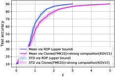
Refer to caption
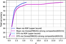
(a) Privacy-Utility trade-offs on the MNIST dataset with subscript\ell_{\infty}-norm clipping.
Refer to caption
(b) Privacy-Utility trade-offs on the MNIST dataset with 2subscript2\ell_{2}-norm clipping.
Figure 5: Distributed private learning.

In Figure 5(a), we choose uniformly at random 10,0001000010,000 clients at each step of the Algorithm 1, where each client clips the subscript\ell_{\infty}-norm of the gradient with clipping parameter C=1/100𝐶1100C=1/100 and applies the subscript\mathcal{R}_{\infty} ϵ0subscriptitalic-ϵ0\epsilon_{0}-LDP mechanism proposed in [GDD+21b] with ϵ0=1.5subscriptitalic-ϵ01.5\epsilon_{0}=1.5. We run Algorithm 1 with δ=105𝛿superscript105\delta=10^{-5} for 200200200 epochs, with learning rate η=0.3𝜂0.3\eta=0.3 for the first 707070 epochs, and then decrease it to 0.180.180.18 in the remaining epochs. Figure 5(a) plots the mean and the standard deviation of privacy-accuracy trade-offs averaged over 101010 runs for subscript\ell_{\infty}-norm clipping.

In Figure 5(b), we choose uniformly at random 2,00020002,000 clients at each step of the Algorithm 1, where each client clips the 2subscript2\ell_{2}-norm of the gradient with clipping parameter C=0.005𝐶0.005C=0.005 and applies the 2subscript2\mathcal{R}_{2} ϵ0subscriptitalic-ϵ0\epsilon_{0}-LDP mechanism (PrivUnit) proposed in [DJW13] with ϵ0=2subscriptitalic-ϵ02\epsilon_{0}=2. We run Algorithm 1 with δ=105𝛿superscript105\delta=10^{-5} for 200200200 epochs, with learning rate η=12𝜂12\eta=12 for the first 303030 epochs, and then decrease it to 444 in the next 303030 epochs. We decrease the learning rate to 3.53.53.5 for the remaining epochs. Figure 5(b) plots the mean and the standard deviation of privacy-accuracy trade-offs averaged over 444 runs for 2subscript2\ell_{2}-norm clipping.

For our privacy analysis, the total privacy budget is computed by optimizing over RDP order λ𝜆\lambda using our upper bound given in Theorem 1. For privacy analysis of [FMT20], we first compute the privacy amplification by shuffling numerically given in [FMT20]; then we compute its privacy obtained when amplified via subsampling [Ull17]; and finally we use the strong composition theorem [KOV15] to obtain the central privacy parameter ϵitalic-ϵ\epsilon.

For the subscript\ell_{\infty}-norm clipping, we achieve an accuracy of 80%(±1.8)percent80plus-or-minus1.880\%(\pm 1.8) with a total privacy budget of ϵ=1.4italic-ϵ1.4\epsilon=1.4 using our new privacy analysis, whereas, [FMT20] achieves an accuracy of 70.7%(±2.1)percent70.7plus-or-minus2.170.7\%(\pm 2.1) with the same privacy budget of ϵ=1.4italic-ϵ1.4\epsilon=1.4 using the standard composition theorems. Furthermore, we achieve an accuracy of 90%(±0.5)percent90plus-or-minus0.590\%(\pm 0.5) with total privacy budget of ϵ=2.91italic-ϵ2.91\epsilon=2.91 using our new privacy analysis, whereas, [FMT20] (together with the standard strong composition theorem) achieve the same accuracy with a total privacy budget of ϵ=4.82italic-ϵ4.82\epsilon=4.82. Similarly, for 2subscript2\ell_{2}-norm clipping, we achieve an accuracy of 81.15%(±0.7)percent81.15plus-or-minus0.781.15\%(\pm 0.7) with a total privacy budget of ϵ=3italic-ϵ3\epsilon=3 using our new privacy analysis, whereas, [FMT20] achieves an accuracy of only 76.46%(±1.9)percent76.46plus-or-minus1.976.46\%(\pm 1.9) with the same privacy budget of ϵ=3italic-ϵ3\epsilon=3 using the standard composition theorems. Furthermore, we achieve an accuracy of 89.7%(±0.5)percent89.7plus-or-minus0.589.7\%(\pm 0.5) with a total privacy budget of ϵ=5.8italic-ϵ5.8\epsilon=5.8 using our new privacy analysis, whereas, [FMT20] (together with the standard strong composition theorem) achieve the same accuracy with a total privacy budget of ϵ=18.3italic-ϵ18.3\epsilon=18.3.

5 Proof of Theorem 1: Upper Bound

For any dataset 𝒟k=(d1,,dk)𝒳ksubscript𝒟𝑘subscript𝑑1subscript𝑑𝑘superscript𝒳𝑘\mathcal{D}_{k}=(d_{1},\ldots,d_{k})\in\mathcal{X}^{k} containing of k𝑘k data points, we define a shuffle mechanism sh(𝒟k)subscript𝑠subscript𝒟𝑘\mathcal{M}_{sh}(\mathcal{D}_{k}) as follows:

sh(𝒟k)=k((d1),,(dk)),subscript𝑠subscript𝒟𝑘subscript𝑘subscript𝑑1subscript𝑑𝑘\mathcal{M}_{sh}(\mathcal{D}_{k})=\mathcal{H}_{k}\left(\mathcal{R}\left(d_{1}\right),\ldots,\mathcal{R}\left(d_{k}\right)\right), (10)

where ksubscript𝑘\mathcal{H}_{k} takes k𝑘k inputs and outputs a uniformly random permutation of them. Recall from (5), for any dataset 𝒟n=(d1,,dn)𝒳nsubscript𝒟𝑛subscript𝑑1subscript𝑑𝑛superscript𝒳𝑛\mathcal{D}_{n}=(d_{1},\ldots,d_{n})\in\mathcal{X}^{n} containing n𝑛n data points, the subsampled-shuffle mechanism is defined as (𝒟):=ksampkn((d1),,(dn))assign𝒟subscript𝑘superscriptsubscriptsamp𝑘𝑛subscript𝑑1subscript𝑑𝑛\mathcal{M}\left(\mathcal{D}\right):=\mathcal{H}_{k}\circ\mathrm{samp}_{k}^{n}\left(\mathcal{R}\left(d_{1}\right),\ldots,\mathcal{R}\left(d_{n}\right)\right).

The proof of Theorem 1 consists of two steps. First, we bound the ternary-|χ|αsuperscript𝜒𝛼|\chi|^{\alpha}-DP of the shuffle mechanism shsubscript𝑠\mathcal{M}_{sh} (see Theorem 4), which is the main technical contribution in this proof. Then, using this, we bound the RDP of the subsampled shuffle mechanism \mathcal{M}.

Theorem 4 (ζ𝜁\zeta-ternary-|χ|αsuperscript𝜒𝛼|\chi|^{\alpha}-DP of the shuffle mechanism shsubscript𝑠\mathcal{M}_{sh}).

For any integer k2𝑘2k\geq 2, ϵ0>0subscriptitalic-ϵ00\epsilon_{0}>0, and all α2𝛼2\alpha\geq 2, the ζ𝜁\zeta-ternary-|χ|αsuperscript𝜒𝛼|\chi|^{\alpha}-DP of the shuffle mechanism shsubscript𝑠\mathcal{M}_{sh} is bounded by:

ζ(α)α{4(eϵ01)2k¯eϵ0+(eϵ0eϵ0)αek18eϵ0if α=2,αΓ(α/2)(2(e2ϵ01)2k¯e2ϵ0)α/2+(eϵ0eϵ0)αek18eϵ0otherwise,𝜁superscript𝛼𝛼cases4superscriptsuperscript𝑒subscriptitalic-ϵ012¯𝑘superscript𝑒subscriptitalic-ϵ0superscriptsuperscript𝑒subscriptitalic-ϵ0superscript𝑒subscriptitalic-ϵ0𝛼superscript𝑒𝑘18superscript𝑒subscriptitalic-ϵ0if 𝛼2𝛼Γ𝛼2superscript2superscriptsuperscript𝑒2subscriptitalic-ϵ012¯𝑘superscript𝑒2subscriptitalic-ϵ0𝛼2superscriptsuperscript𝑒subscriptitalic-ϵ0superscript𝑒subscriptitalic-ϵ0𝛼superscript𝑒𝑘18superscript𝑒subscriptitalic-ϵ0otherwise\zeta\left(\alpha\right)^{\alpha}\leq\left\{\begin{array}[]{ll}4\frac{\left(e^{\epsilon_{0}}-1\right)^{2}}{\overline{k}e^{\epsilon_{0}}}+(e^{\epsilon_{0}}-e^{-\epsilon_{0}})^{\alpha}e^{-\frac{k-1}{8e^{\epsilon_{0}}}}&\text{if\ }\alpha=2,\\ \alpha\Gamma\left(\alpha/2\right)\left(\frac{2\left(e^{2\epsilon_{0}}-1\right)^{2}}{\overline{k}e^{2\epsilon_{0}}}\right)^{\alpha/2}+(e^{\epsilon_{0}}-e^{-\epsilon_{0}})^{\alpha}e^{-\frac{k-1}{8e^{\epsilon_{0}}}}&\text{otherwise},\end{array}\right. (11)

where k¯=k12eϵ0+1¯𝑘𝑘12superscript𝑒subscriptitalic-ϵ01\overline{k}=\lfloor\frac{k-1}{2e^{\epsilon_{0}}}\rfloor+1 and Γ(z)=0xz1ex𝑑xΓ𝑧superscriptsubscript0superscript𝑥𝑧1superscript𝑒𝑥differential-d𝑥\Gamma\left(z\right)=\int_{0}^{\infty}x^{z-1}e^{-x}dx is the Gamma function.

Theorem 4 is one of the core technical results of this paper, and we prove it in Section 6.

It was shown in [WBK19, Proposition 161616] that if a mechanism obeys ζ𝜁\zeta-ternary-|χ|αsuperscript𝜒𝛼|\chi|^{\alpha}-DP, then its subsampled version (with subsampling parameter γ𝛾\gamma) will obey γζ𝛾𝜁\gamma\zeta-ternary-|χ|αsuperscript𝜒𝛼|\chi|^{\alpha}-DP. Using that result, the authors then bounded the RDP of the subsampled mechanism in [WBK19, Eq. (9)9(9)]. Adapting that result to our setting, we have the following lemma.

Lemma 2 (From ζ𝜁\zeta-ternary-|χ|αsuperscript𝜒𝛼|\chi|^{\alpha}-DP to subsampled RDP).

Suppose the shuffle mechanism shsubscript𝑠\mathcal{M}_{sh} obeys ζ𝜁\zeta-ternary-|χ|αsuperscript𝜒𝛼|\chi|^{\alpha}-DP. For any λ2,knformulae-sequence𝜆2𝑘𝑛\lambda\geq 2,k\leq n, RDP of the subsampled shuffle mechanism \mathcal{M} (with subsampling parameter γ=k/n𝛾𝑘𝑛\gamma=k/n) is bounded by: ϵ(λ)1λ1log(1+α=2λ(λα)γαζ(α)α)italic-ϵ𝜆1𝜆11superscriptsubscript𝛼2𝜆binomial𝜆𝛼superscript𝛾𝛼𝜁superscript𝛼𝛼\epsilon(\lambda)\leq\frac{1}{\lambda-1}\log\big{(}1+\sum_{\alpha=2}^{\lambda}\binom{\lambda}{\alpha}\gamma^{\alpha}\zeta(\alpha)^{\alpha}\big{)}.

Lemma 2 can be seen as a corollary to [WBK19, Proposition 161616 and Eq. (9)9(9)]. However, for completeness, we prove it in Appendix C. Substituting the bound on ζ(α)𝜁𝛼\zeta(\alpha) from Theorem 4 into Lemma 2, we get

ϵ(λ)italic-ϵ𝜆\displaystyle\epsilon\left(\lambda\right) 1λ1log[1+(λ2)γ2(4(eϵ01)2k¯eϵ0+(eϵ0eϵ0)2ek18eϵ0)\displaystyle\leq\frac{1}{\lambda-1}\log\left[1+\binom{\lambda}{2}\gamma^{2}\left(4\frac{\left(e^{\epsilon_{0}}-1\right)^{2}}{\overline{k}e^{\epsilon_{0}}}+(e^{\epsilon_{0}}-e^{-\epsilon_{0}})^{2}e^{-\frac{k-1}{8e^{\epsilon_{0}}}}\right)\right.
+α=3λ(λα)γα(αΓ(α/2)(2(e2ϵ01)2k¯e2ϵ0)α/2+(eϵ0eϵ0)αek18eϵ0)]\displaystyle\hskip 71.13188pt\left.+\sum_{\alpha=3}^{\lambda}\binom{\lambda}{\alpha}\gamma^{\alpha}\left(\alpha\Gamma(\alpha/2)\left(\frac{2\left(e^{2\epsilon_{0}}-1\right)^{2}}{\overline{k}e^{2\epsilon_{0}}}\right)^{\alpha/2}+(e^{\epsilon_{0}}-e^{-\epsilon_{0}})^{\alpha}e^{-\frac{k-1}{8e^{\epsilon_{0}}}}\right)\right]
=1λ1log[1+4(λ2)γ2(eϵ01)2k¯eϵ0+α=3λ(λα)γααΓ(α/2)(2(e2ϵ01)2k¯e2ϵ0)α/2+Υ],absent1𝜆114binomial𝜆2superscript𝛾2superscriptsuperscript𝑒subscriptitalic-ϵ012¯𝑘superscript𝑒subscriptitalic-ϵ0superscriptsubscript𝛼3𝜆binomial𝜆𝛼superscript𝛾𝛼𝛼Γ𝛼2superscript2superscriptsuperscript𝑒2subscriptitalic-ϵ012¯𝑘superscript𝑒2subscriptitalic-ϵ0𝛼2Υ\displaystyle=\frac{1}{\lambda-1}\log\left[1+4\binom{\lambda}{2}\gamma^{2}\frac{\left(e^{\epsilon_{0}}-1\right)^{2}}{\overline{k}e^{\epsilon_{0}}}+\sum_{\alpha=3}^{\lambda}\binom{\lambda}{\alpha}\gamma^{\alpha}\alpha\Gamma(\alpha/2)\left(\frac{2\left(e^{2\epsilon_{0}}-1\right)^{2}}{\overline{k}e^{2\epsilon_{0}}}\right)^{\alpha/2}+\Upsilon\right], (12)

where Υ=α=2λ(λα)γα(eϵ0eϵ0)αek18eϵ0=((1+γe2ϵ01eϵ0)λ1λγe2ϵ01eϵ0)ek18eϵ0Υsuperscriptsubscript𝛼2𝜆binomial𝜆𝛼superscript𝛾𝛼superscriptsuperscript𝑒subscriptitalic-ϵ0superscript𝑒subscriptitalic-ϵ0𝛼superscript𝑒𝑘18superscript𝑒subscriptitalic-ϵ0superscript1𝛾superscript𝑒2subscriptitalic-ϵ01superscript𝑒subscriptitalic-ϵ0𝜆1𝜆𝛾superscript𝑒2subscriptitalic-ϵ01superscript𝑒subscriptitalic-ϵ0superscript𝑒𝑘18superscript𝑒subscriptitalic-ϵ0\Upsilon=\sum_{\alpha=2}^{\lambda}\binom{\lambda}{\alpha}\gamma^{\alpha}(e^{\epsilon_{0}}-e^{-\epsilon_{0}})^{\alpha}e^{-\frac{k-1}{8e^{\epsilon_{0}}}}=\left(\left(1+\gamma\frac{e^{2\epsilon_{0}}-1}{e^{\epsilon_{0}}}\right)^{\lambda}-1-\lambda\gamma\frac{e^{2\epsilon_{0}}-1}{e^{\epsilon_{0}}}\right)e^{-\frac{k-1}{8e^{\epsilon_{0}}}}.

The above expression in (12) is the bound given in Theorem 1.

6 Proof of Theorem 4: Ternary |χ|αsuperscript𝜒𝛼|\chi|^{\alpha}-DP of the Shuffle Model

The proof has two main steps. In the first step, we reduce the problem of deriving ternary divergence for arbitrary neighboring datasets to the problem of deriving the ternary divergence for specific neighboring datasets, 𝒟𝒟𝒟′′similar-to𝒟superscript𝒟similar-tosuperscript𝒟′′\mathcal{D}\sim\mathcal{D}^{\prime}\sim\mathcal{D}^{\prime\prime}, where all elements in 𝒟𝒟\mathcal{D} are the same and 𝒟,𝒟′′superscript𝒟superscript𝒟′′\mathcal{D}^{\prime},\mathcal{D}^{\prime\prime} differ from 𝒟𝒟\mathcal{D} in one entry. In the second step, we derive the ternary divergence for the special neighboring datasets.

The specific neighboring datasets to which we reduce our general problem has the following form:

𝒟samemsuperscriptsubscript𝒟same𝑚\displaystyle\mathcal{D}_{\text{same}}^{m} ={(𝒟m,𝒟m,𝒟m′′):𝒟m=(d,,d,d)𝒳m,𝒟m=(d,,d,d)𝒳m, and \displaystyle=\left\{(\mathcal{D}_{m},\mathcal{D}^{\prime}_{m},\mathcal{D}^{\prime\prime}_{m}):\mathcal{D}_{m}=(d,\ldots,d,d)\in\mathcal{X}^{m},\ \mathcal{D}^{\prime}_{m}=(d,\ldots,d,d^{\prime})\in\mathcal{X}^{m},\text{ and }\right.
𝒟m′′=(d,,d,d′′)𝒳m, where d,d,d′′𝒳},\displaystyle\left.\hskip 113.81102pt\mathcal{D}^{\prime\prime}_{m}=(d,\ldots,d,d^{\prime\prime})\in\mathcal{X}^{m},\text{ where }d,d^{\prime},d^{\prime\prime}\in\mathcal{X}\right\}, (13)

Consider arbitrary neighboring datasets 𝒟=(d1,,dk1,dk)𝒟subscript𝑑1subscript𝑑𝑘1subscript𝑑𝑘\mathcal{D}=(d_{1},\ldots,d_{k-1},d_{k}), 𝒟=(d1,,dk1,dk)superscript𝒟subscript𝑑1subscript𝑑𝑘1subscriptsuperscript𝑑𝑘\mathcal{D}^{\prime}=(d_{1},\ldots,d_{k-1},d^{\prime}_{k}), 𝒟′′=(d1,,dk1,dk′′)superscript𝒟′′subscript𝑑1subscript𝑑𝑘1subscriptsuperscript𝑑′′𝑘\mathcal{D}^{\prime\prime}=(d_{1},\ldots,d_{k-1},d^{\prime\prime}_{k}), each having k𝑘k elements. For any m{0,,k1}𝑚0𝑘1m\in\{0,\ldots,k-1\}, we define new neighboring datasets 𝒟m+1(k)=(dk′′,,dk′′,dk)superscriptsubscript𝒟𝑚1𝑘subscriptsuperscript𝑑′′𝑘subscriptsuperscript𝑑′′𝑘subscript𝑑𝑘\mathcal{D}_{m+1}^{(k)}=(d^{\prime\prime}_{k},\ldots,d^{\prime\prime}_{k},d_{k}), 𝒟m+1(k)=(dk′′,,dk′′,dk)subscriptsuperscript𝒟𝑘𝑚1subscriptsuperscript𝑑′′𝑘subscriptsuperscript𝑑′′𝑘subscriptsuperscript𝑑𝑘\mathcal{D}^{\prime(k)}_{m+1}=(d^{\prime\prime}_{k},\ldots,d^{\prime\prime}_{k},d^{\prime}_{k}), and 𝒟m+1′′(k)=(dk′′,,dk′′)subscriptsuperscript𝒟′′𝑘𝑚1subscriptsuperscript𝑑′′𝑘subscriptsuperscript𝑑′′𝑘\mathcal{D}^{\prime\prime(k)}_{m+1}=(d^{\prime\prime}_{k},\ldots,d^{\prime\prime}_{k}), each having m+1𝑚1m+1 elements. Observe that (𝒟m+1′′(k),𝒟m+1(k),𝒟m+1(k))𝒟samemsubscriptsuperscript𝒟′′𝑘𝑚1subscriptsuperscript𝒟𝑘𝑚1subscriptsuperscript𝒟𝑘𝑚1superscriptsubscript𝒟same𝑚(\mathcal{D}^{\prime\prime(k)}_{m+1},\mathcal{D}^{\prime(k)}_{m+1},\mathcal{D}^{(k)}_{m+1})\in\mathcal{D}_{\text{same}}^{m}. The first step of the proof is given in the following theorem:

Theorem 5 (Reduction to the Special Case).

Let q=1eϵ0𝑞1superscript𝑒subscriptitalic-ϵ0q=\frac{1}{e^{\epsilon_{0}}}. We have:

𝔼𝒉sh(𝒟′′)[|sh(𝒟)(𝒉)sh(𝒟)(𝒉)sh(𝒟′′)(𝒉)|α]subscript𝔼similar-to𝒉subscript𝑠superscript𝒟′′delimited-[]superscriptsubscript𝑠𝒟𝒉subscript𝑠superscript𝒟𝒉subscript𝑠superscript𝒟′′𝒉𝛼\displaystyle\mathbb{E}_{\boldsymbol{h}\sim\mathcal{M}_{sh}(\mathcal{D}^{\prime\prime})}\left[\left|\frac{\mathcal{M}_{sh}(\mathcal{D})(\boldsymbol{h})-\mathcal{M}_{sh}(\mathcal{D}^{\prime})(\boldsymbol{h})}{\mathcal{M}_{sh}(\mathcal{D}^{\prime\prime})(\boldsymbol{h})}\right|^{\alpha}\right]
𝔼mBin(k1,q)[𝔼𝒉sh(𝒟m+1′′(k))[|sh(𝒟m+1(k))(𝒉)sh(𝒟m+1(k))(𝒉)sh(𝒟m+1′′(k))(𝒉)|α]].absentsubscript𝔼similar-to𝑚Bin𝑘1𝑞delimited-[]subscript𝔼similar-to𝒉subscript𝑠superscriptsubscript𝒟𝑚1′′𝑘delimited-[]superscriptsubscript𝑠superscriptsubscript𝒟𝑚1𝑘𝒉subscript𝑠superscriptsubscript𝒟𝑚1𝑘𝒉subscript𝑠superscriptsubscript𝒟𝑚1′′𝑘𝒉𝛼\displaystyle\hskip 28.45274pt\leq\mathbb{E}_{m\sim\emph{Bin}\left(k-1,q\right)}\left[\mathbb{E}_{\boldsymbol{h}\sim\mathcal{M}_{sh}(\mathcal{D}_{m+1}^{\prime\prime(k)})}\left[\left|\frac{\mathcal{M}_{sh}(\mathcal{D}_{m+1}^{(k)})(\boldsymbol{h})-\mathcal{M}_{sh}(\mathcal{D}_{m+1}^{\prime(k)})(\boldsymbol{h})}{\mathcal{M}_{sh}(\mathcal{D}_{m+1}^{\prime\prime(k)})(\boldsymbol{h})}\right|^{\alpha}\right]\right]. (14)

We present a proof of Theorem 5 in Section 6.1. We know (by Chernoff bound) that the binomial r.v. is concentrated around its mean, which implies that the terms in the RHS of (14) that correspond to m<(1τ)q(k1)𝑚1𝜏𝑞𝑘1m<(1-\tau)q(k-1) (we will take τ=1/2𝜏12\tau=1/2) will contribute in a negligible amount. Then we show that Em:=𝔼𝒉sh(𝒟m+1′′(k))[|sh(𝒟m+1(k))(𝒉)sh(𝒟m+1(k))(𝒉)sh(𝒟m+1′′(k))(𝒉)|α]assignsubscript𝐸𝑚subscript𝔼similar-to𝒉subscript𝑠superscriptsubscript𝒟𝑚1′′𝑘delimited-[]superscriptsubscript𝑠superscriptsubscript𝒟𝑚1𝑘𝒉subscript𝑠superscriptsubscript𝒟𝑚1𝑘𝒉subscript𝑠superscriptsubscript𝒟𝑚1′′𝑘𝒉𝛼E_{m}:=\mathbb{E}_{\boldsymbol{h}\sim\mathcal{M}_{sh}(\mathcal{D}_{m+1}^{\prime\prime(k)})}\left[\left|\frac{\mathcal{M}_{sh}(\mathcal{D}_{m+1}^{(k)})(\boldsymbol{h})-\mathcal{M}_{sh}(\mathcal{D}_{m+1}^{\prime(k)})(\boldsymbol{h})}{\mathcal{M}_{sh}(\mathcal{D}_{m+1}^{\prime\prime(k)})(\boldsymbol{h})}\right|^{\alpha}\right] is a non-increasing function of m𝑚m. These observation together imply that the RHS in (14) is approximately upper bounded by E(1τ)q(k1)subscript𝐸1𝜏𝑞𝑘1E_{(1-\tau)q(k-1)}.

Since Emsubscript𝐸𝑚E_{m} is precisely what is required to bound the ternary DP for the specific neighboring datasets, we have reduced the problem of computing the ternary DP for arbitrary neighboring datasets to the problem of computing ternary DP for specific neighboring datasets. The second step of the proof bounds E(1τ)q(n1)subscript𝐸1𝜏𝑞𝑛1E_{(1-\tau)q(n-1)}, which follows from the result below that holds for any m𝑚m\in\mathbb{N}.

Theorem 6 (|χ|αsuperscript𝜒𝛼|\chi|^{\alpha}-DP for special case).

For any m𝑚m\in\mathbb{N}, integer α2𝛼2\alpha\geq 2, and (𝒟m′′,𝒟m,𝒟m)𝒟samemsubscriptsuperscript𝒟′′𝑚subscriptsuperscript𝒟𝑚subscript𝒟𝑚superscriptsubscript𝒟same𝑚(\mathcal{D}^{\prime\prime}_{m},\mathcal{D}^{\prime}_{m},\mathcal{D}_{m})\in\mathcal{D}_{\text{same}}^{m},

𝔼𝒉sh(𝒟m)[|sh(𝒟m)(𝒉)sh(𝒟m′′)(𝒉)sh(𝒟m)(𝒉)|α]{4(eϵ01)2meϵ0if α=2,αΓ(α/2)(2(e2ϵ01)2me2ϵ0)α/2otherwise.subscript𝔼similar-to𝒉subscript𝑠subscript𝒟𝑚delimited-[]superscriptsubscript𝑠subscriptsuperscript𝒟𝑚𝒉subscript𝑠subscriptsuperscript𝒟′′𝑚𝒉subscript𝑠subscript𝒟𝑚𝒉𝛼cases4superscriptsuperscript𝑒subscriptitalic-ϵ012𝑚superscript𝑒subscriptitalic-ϵ0if 𝛼2𝛼Γ𝛼2superscript2superscriptsuperscript𝑒2subscriptitalic-ϵ012𝑚superscript𝑒2subscriptitalic-ϵ0𝛼2otherwise\displaystyle\mathbb{E}_{\boldsymbol{h}\sim\mathcal{M}_{sh}(\mathcal{D}_{m})}\left[\left|\frac{\mathcal{M}_{sh}(\mathcal{D}^{\prime}_{m})(\boldsymbol{h})-\mathcal{M}_{sh}(\mathcal{D}^{\prime\prime}_{m})(\boldsymbol{h})}{\mathcal{M}_{sh}(\mathcal{D}_{m})(\boldsymbol{h})}\right|^{\alpha}\right]\leq\left\{\begin{array}[]{ll}4\frac{\left(e^{\epsilon_{0}}-1\right)^{2}}{me^{\epsilon_{0}}}&\text{if\ }\alpha=2,\\ \alpha\Gamma(\alpha/2)\left(\frac{2(e^{2\epsilon_{0}}-1)^{2}}{me^{2\epsilon_{0}}}\right)^{\alpha/2}&\text{otherwise}.\end{array}\right.

The proof of Theorem 6 is presented in Section 6.2. Missing details of how Theorem 4 follows from Theorems 5, 6 can be found in Appendix B.

6.1 Proof of Theorem 5: Reduction to the Special Case

First, we prove the joint-convexity of the ternary |χ|αsuperscript𝜒𝛼|\chi|^{\alpha}-divergence as it is important in the following proof.

Lemma 3 (Joint-convexity of the ternary |χ|αsuperscript𝜒𝛼|\chi|^{\alpha}-divergence).

For all α1𝛼1\alpha\geq 1, the ternary-|χ|αsuperscript𝜒𝛼|\chi|^{\alpha}-divergence 𝔼[|PQR|α]𝔼delimited-[]superscript𝑃𝑄𝑅𝛼\mathbb{E}\left[\left|\frac{P-Q}{R}\right|^{\alpha}\right] is jointly convex in P,Q𝑃𝑄P,Q and R𝑅R. In other words, if Pa=aP0+(1a)P1subscript𝑃𝑎𝑎subscript𝑃01𝑎subscript𝑃1P_{a}=aP_{0}+(1-a)P_{1}, Qa=aQ0+(1a)Q1subscript𝑄𝑎𝑎subscript𝑄01𝑎subscript𝑄1Q_{a}=aQ_{0}+(1-a)Q_{1}, and Ra=aR0+(1a)R1subscript𝑅𝑎𝑎subscript𝑅01𝑎subscript𝑅1R_{a}=aR_{0}+(1-a)R_{1} for some a[0,1]𝑎01a\in\left[0,1\right], then the following holds

𝔼[|PaQaRa|α]a𝔼[|P0Q0R0|α]+(1a)𝔼[|P1Q1R1|α]𝔼delimited-[]superscriptsubscript𝑃𝑎subscript𝑄𝑎subscript𝑅𝑎𝛼𝑎𝔼delimited-[]superscriptsubscript𝑃0subscript𝑄0subscript𝑅0𝛼1𝑎𝔼delimited-[]superscriptsubscript𝑃1subscript𝑄1subscript𝑅1𝛼\mathbb{E}\left[\left|\frac{P_{a}-Q_{a}}{R_{a}}\right|^{\alpha}\right]\leq a\mathbb{E}\left[\left|\frac{P_{0}-Q_{0}}{R_{0}}\right|^{\alpha}\right]+(1-a)\mathbb{E}\left[\left|\frac{P_{1}-Q_{1}}{R_{1}}\right|^{\alpha}\right] (15)
Proof.

First, observe that g(x,y)=|xy|𝑔𝑥𝑦𝑥𝑦g(x,y)=|x-y| is jointly convex on 2superscript2\mathbb{R}^{2}, i.e., if xa=ax0+(1a)x1subscript𝑥𝑎𝑎subscript𝑥01𝑎subscript𝑥1x_{a}=ax_{0}+(1-a)x_{1} and ya=ay0+(1a)y1subscript𝑦𝑎𝑎subscript𝑦01𝑎subscript𝑦1y_{a}=ay_{0}+(1-a)y_{1}, we have

|xaya|subscript𝑥𝑎subscript𝑦𝑎\displaystyle|x_{a}-y_{a}| =|a(x0y0)+(1a)(x1y1)|absent𝑎subscript𝑥0subscript𝑦01𝑎subscript𝑥1subscript𝑦1\displaystyle=|a(x_{0}-y_{0})+(1-a)(x_{1}-y_{1})|
a|x0y0|+(1a)|x1y1|absent𝑎subscript𝑥0subscript𝑦01𝑎subscript𝑥1subscript𝑦1\displaystyle\leq a|x_{0}-y_{0}|+(1-a)|x_{1}-y_{1}| (16)

Let f(x,y)=xj/yj1𝑓𝑥𝑦superscript𝑥𝑗superscript𝑦𝑗1f(x,y)=x^{j}/y^{j-1}, which is jointly convex on +2superscriptsubscript2\mathbb{R}_{+}^{2} for j1𝑗1j\geq 1; see [WBK19, Lemma 202020] for a proof. Thus, we get

|PaQa|jRaj1superscriptsubscript𝑃𝑎subscript𝑄𝑎𝑗superscriptsubscript𝑅𝑎𝑗1\displaystyle\frac{|P_{a}-Q_{a}|^{j}}{R_{a}^{j-1}} (a|P0Q0|+(1a)|P1Q1|)j(aR0+(1a)R1)j1absentsuperscript𝑎subscript𝑃0subscript𝑄01𝑎subscript𝑃1subscript𝑄1𝑗superscript𝑎subscript𝑅01𝑎subscript𝑅1𝑗1\displaystyle\leq\frac{\left(a|P_{0}-Q_{0}|+(1-a)|P_{1}-Q_{1}|\right)^{j}}{(aR_{0}+(1-a)R_{1})^{j-1}} a|P0Q0|jR0j1+(1a)|P1Q1|jR1j1,absent𝑎superscriptsubscript𝑃0subscript𝑄0𝑗superscriptsubscript𝑅0𝑗11𝑎superscriptsubscript𝑃1subscript𝑄1𝑗superscriptsubscript𝑅1𝑗1\displaystyle\leq a\frac{|P_{0}-Q_{0}|^{j}}{R_{0}^{j-1}}+(1-a)\frac{|P_{1}-Q_{1}|^{j}}{R_{1}^{j-1}}, (17)

where the first inequality is obtained from (16) and the second inequality is obtained from the convexity of f(x,y)𝑓𝑥𝑦f(x,y). ∎

Now, we prove Theorem 5. Our proof is an adaptation of the proof of  [GDD+21a, Theorem 444]. The difference comes from the fact that [GDD+21a, Theorem 444] was for Renyi divergence, whereas, here we are working with ternary |χ|αsuperscript𝜒𝛼|\chi|^{\alpha}-divergence. This changes some details and we provide a full proof of Theorem 5 below.

Let 𝒑i:=(pi1,,piB)assignsubscript𝒑𝑖subscript𝑝𝑖1subscript𝑝𝑖𝐵\boldsymbol{p}_{i}:=(p_{i1},\ldots,p_{iB}), 𝒑k:=(pk1,,pkB)assignsubscriptsuperscript𝒑𝑘subscriptsuperscript𝑝𝑘1subscriptsuperscript𝑝𝑘𝐵\boldsymbol{p}^{\prime}_{k}:=(p^{\prime}_{k1},\ldots,p^{\prime}_{kB}), 𝒑k′′:=(pk1′′,,pkB′′)assignsubscriptsuperscript𝒑′′𝑘subscriptsuperscript𝑝′′𝑘1subscriptsuperscript𝑝′′𝑘𝐵\boldsymbol{p}^{\prime\prime}_{k}:=(p^{\prime\prime}_{k1},\ldots,p^{\prime\prime}_{kB}) denote the probability distributions over 𝒴𝒴\mathcal{Y} when the input to \mathcal{R} is disubscript𝑑𝑖d_{i}, dksubscriptsuperscript𝑑𝑘d^{\prime}_{k}, and dk′′subscriptsuperscript𝑑′′𝑘d^{\prime\prime}_{k} respectively, where pij=Pr[(di)=j]subscript𝑝𝑖𝑗Prsubscript𝑑𝑖𝑗p_{ij}=\Pr[\mathcal{R}(d_{i})=j] for all j[B]𝑗delimited-[]𝐵j\in[B] and i[n]𝑖delimited-[]𝑛i\in\left[n\right]. Let 𝒫={𝒑i:i[k]}𝒫conditional-setsubscript𝒑𝑖𝑖delimited-[]𝑘\mathcal{P}=\{\boldsymbol{p}_{i}:i\in\left[k\right]\}, 𝒫={𝒑i:i[k1]}{𝒑k}superscript𝒫conditional-setsubscript𝒑𝑖𝑖delimited-[]𝑘1subscriptsuperscript𝒑𝑘\mathcal{P}^{\prime}=\{\boldsymbol{p}_{i}:i\in\left[k-1\right]\}\bigcup\{\boldsymbol{p}^{\prime}_{k}\}, and 𝒫′′={𝒑i:i[k1]}{𝒑k′′}superscript𝒫′′conditional-setsubscript𝒑𝑖𝑖delimited-[]𝑘1subscriptsuperscript𝒑′′𝑘\mathcal{P}^{\prime\prime}=\{\boldsymbol{p}_{i}:i\in\left[k-1\right]\}\bigcup\{\boldsymbol{p}^{\prime\prime}_{k}\}.

For i[k1]𝑖delimited-[]𝑘1i\in[k-1], let 𝒫i=𝒫{𝒑i}subscript𝒫𝑖𝒫subscript𝒑𝑖\mathcal{P}_{-i}=\mathcal{P}\setminus\{\boldsymbol{p}_{i}\} and also 𝒫k=𝒫{𝒑k}subscript𝒫𝑘𝒫subscript𝒑𝑘\mathcal{P}_{-k}=\mathcal{P}\setminus\{\boldsymbol{p}_{k}\}. Here, 𝒫,𝒫,𝒫′′𝒫superscript𝒫superscript𝒫′′\mathcal{P},\mathcal{P}^{\prime},\mathcal{P}^{\prime\prime} correspond to the datasets 𝒟={d1,,dk},𝒟={d1,,dk1,dk}formulae-sequence𝒟subscript𝑑1subscript𝑑𝑘superscript𝒟subscript𝑑1subscript𝑑𝑘1subscriptsuperscript𝑑𝑘\mathcal{D}=\{d_{1},\ldots,d_{k}\},\mathcal{D}^{\prime}=\{d_{1},\ldots,d_{k-1},d^{\prime}_{k}\}, and 𝒟′′={d1,,dk1,dk′′}superscript𝒟′′subscript𝑑1subscript𝑑𝑘1subscriptsuperscript𝑑′′𝑘\mathcal{D}^{\prime\prime}=\{d_{1},\ldots,d_{k-1},d^{\prime\prime}_{k}\} respectively, and for any i[k]𝑖delimited-[]𝑘i\in[k], 𝒫isubscript𝒫𝑖\mathcal{P}_{-i} corresponds to the dataset 𝒟i={d1,,di1,di+1,,dk}subscript𝒟𝑖subscript𝑑1subscript𝑑𝑖1subscript𝑑𝑖1subscript𝑑𝑘\mathcal{D}_{-i}=\{d_{1},\ldots,d_{i-1},d_{i+1},\ldots,d_{k}\}.

For any collection 𝒫={𝒑1,,𝒑k}𝒫subscript𝒑1subscript𝒑𝑘\mathcal{P}=\{\boldsymbol{p}_{1},\ldots,\boldsymbol{p}_{k}\} of k𝑘k distributions, we define F(𝒫)𝐹𝒫F(\mathcal{P}) to be the distribution over 𝒜Bksuperscriptsubscript𝒜𝐵𝑘\mathcal{A}_{B}^{k} (which is the set of histograms on B𝐵B bins with k𝑘k elements as defined in (6)) that is induced when every client i𝑖i (independent to the other clients) samples an element from [B]delimited-[]𝐵[B] accordingly to the probability distribution 𝒑isubscript𝒑𝑖\boldsymbol{p}_{i}. Formally, for any 𝒉𝒜Bk𝒉superscriptsubscript𝒜𝐵𝑘\boldsymbol{h}\in\mathcal{A}_{B}^{k}, define

𝒰𝒉:={(𝒰1,,𝒰B):𝒰1,,𝒰B[k] s.t. j=1B𝒰j=[k] and |𝒰j|=hj,j[B]}.assignsubscript𝒰𝒉conditional-setsubscript𝒰1subscript𝒰𝐵formulae-sequencesubscript𝒰1subscript𝒰𝐵delimited-[]𝑘 s.t. superscriptsubscript𝑗1𝐵subscript𝒰𝑗delimited-[]𝑘 and subscript𝒰𝑗subscript𝑗for-all𝑗delimited-[]𝐵\displaystyle\mathcal{U}_{\boldsymbol{h}}:=\left\{(\mathcal{U}_{1},\ldots,\mathcal{U}_{B}):\mathcal{U}_{1},\ldots,\mathcal{U}_{B}\subseteq[k]\text{ s.t. }\bigcup_{j=1}^{B}\mathcal{U}_{j}=[k]\text{ and }|\mathcal{U}_{j}|=h_{j},\forall j\in[B]\right\}. (18)

Note that for each (𝒰1,,𝒰B)𝒰𝒉subscript𝒰1subscript𝒰𝐵subscript𝒰𝒉(\mathcal{U}_{1},\ldots,\mathcal{U}_{B})\in\mathcal{U}_{\boldsymbol{h}}, 𝒰jsubscript𝒰𝑗\mathcal{U}_{j} for j=1,,B𝑗1𝐵j=1,\ldots,B denotes the identities of the clients that map to the j𝑗j’th element in [B]delimited-[]𝐵[B] – here 𝒰jsubscript𝒰𝑗\mathcal{U}_{j}’s are disjoint for all j[B]𝑗delimited-[]𝐵j\in[B]. Note also that |𝒰𝒉|=(k𝒉)=k!h1!h2!hB!subscript𝒰𝒉binomial𝑘𝒉𝑘subscript1subscript2subscript𝐵|\mathcal{U}_{\boldsymbol{h}}|=\binom{k}{\boldsymbol{h}}=\frac{k!}{h_{1}!h_{2}!\ldots h_{B}!}. It is easy to verify that for any 𝒉𝒜Bk𝒉superscriptsubscript𝒜𝐵𝑘\boldsymbol{h}\in\mathcal{A}_{B}^{k}, F(𝒫)(𝒉)𝐹𝒫𝒉F(\mathcal{P})(\boldsymbol{h}) is equal to

F(𝒫)(𝒉)=(𝒰1,,𝒰B)𝒰𝒉j=1Bi𝒰jpij𝐹𝒫𝒉subscriptsubscript𝒰1subscript𝒰𝐵subscript𝒰𝒉superscriptsubscriptproduct𝑗1𝐵subscriptproduct𝑖subscript𝒰𝑗subscript𝑝𝑖𝑗\displaystyle F(\mathcal{P})(\boldsymbol{h})=\sum_{(\mathcal{U}_{1},\ldots,\mathcal{U}_{B})\in\mathcal{U}_{\boldsymbol{h}}}\prod_{j=1}^{B}\prod_{i\in\mathcal{U}_{j}}p_{ij} (19)

Similarly, we can define F(𝒫),F(𝒫′′),F(𝒫i),F(𝒫i)𝐹superscript𝒫𝐹superscript𝒫′′𝐹subscript𝒫𝑖𝐹subscriptsuperscript𝒫𝑖F(\mathcal{P}^{\prime}),F(\mathcal{P}^{\prime\prime}),F(\mathcal{P}_{-i}),F(\mathcal{P}^{\prime}_{-i}), and F(𝒫i′′)𝐹subscriptsuperscript𝒫′′𝑖F(\mathcal{P}^{\prime\prime}_{-i}). Note that F(𝒫)𝐹𝒫F(\mathcal{P}), F(𝒫)𝐹superscript𝒫F(\mathcal{P}^{\prime}) and F(𝒫′′)𝐹superscript𝒫′′F(\mathcal{P}^{\prime\prime}) are distributions over 𝒜Bksuperscriptsubscript𝒜𝐵𝑘\mathcal{A}_{B}^{k}, whereas, F(𝒫i)𝐹subscript𝒫𝑖F(\mathcal{P}_{-i}), F(𝒫i)𝐹subscriptsuperscript𝒫𝑖F(\mathcal{P}^{\prime}_{-i}), and F(𝒫i′′)𝐹subscriptsuperscript𝒫′′𝑖F(\mathcal{P}^{\prime\prime}_{-i}) are distributions over 𝒜Bk1superscriptsubscript𝒜𝐵𝑘1\mathcal{A}_{B}^{k-1}. It is easy to see that F(𝒫)=sh(𝒟)𝐹𝒫subscript𝑠𝒟F(\mathcal{P})=\mathcal{M}_{sh}(\mathcal{D}), F(𝒫)=sh(𝒟)𝐹superscript𝒫subscript𝑠superscript𝒟F(\mathcal{P}^{\prime})=\mathcal{M}_{sh}(\mathcal{D}^{\prime}), and F(𝒫′′)=sh(𝒟′′)𝐹superscript𝒫′′subscript𝑠superscript𝒟′′F(\mathcal{P}^{\prime\prime})=\mathcal{M}_{sh}(\mathcal{D}^{\prime\prime}).

A crucial observation is that any distribution 𝒑isubscript𝒑𝑖\boldsymbol{p}_{i} can be written as the following mixture distribution:

𝒑i=q𝒑k′′+(1q)𝒑~i,subscript𝒑𝑖𝑞subscriptsuperscript𝒑′′𝑘1𝑞subscript~𝒑𝑖\boldsymbol{p}_{i}=q\boldsymbol{p}^{\prime\prime}_{k}+\left(1-q\right)\tilde{\boldsymbol{p}}_{i}, (20)

where q=1eϵ0𝑞1superscript𝑒subscriptitalic-ϵ0q=\frac{1}{e^{\epsilon_{0}}}. The distribution 𝒑~i=[p~i1,,p~iB]subscript~𝒑𝑖subscript~𝑝𝑖1subscript~𝑝𝑖𝐵\tilde{\boldsymbol{p}}_{i}=\left[\tilde{p}_{i1},\ldots,\tilde{p}_{iB}\right] is given by p~ij=pijqpkj′′1qsubscript~𝑝𝑖𝑗subscript𝑝𝑖𝑗𝑞subscriptsuperscript𝑝′′𝑘𝑗1𝑞\tilde{p}_{ij}=\frac{p_{ij}-qp^{\prime\prime}_{kj}}{1-q}, where it is easy to verify that p~ij0subscript~𝑝𝑖𝑗0\tilde{p}_{ij}\geq 0 and j=1Bp~ij=1superscriptsubscript𝑗1𝐵subscript~𝑝𝑖𝑗1\sum_{j=1}^{B}\tilde{p}_{ij}=1. The idea of writing the distribution of the output of an LDP mechanism as a mixture distribution was previously proposed in [BBGN19c, FMT20]. However, the way these mixture distributions are used in our RDP analysis is quite different from their use in studying the hockey-stick divergence.

For any 𝒞[k1]𝒞delimited-[]𝑘1\mathcal{C}\subseteq[k-1], define three sets 𝒫𝒞,𝒫𝒞subscript𝒫𝒞subscriptsuperscript𝒫𝒞\mathcal{P}_{\mathcal{C}},\mathcal{P}^{\prime}_{\mathcal{C}}, and 𝒫𝒞′′subscriptsuperscript𝒫′′𝒞\mathcal{P}^{\prime\prime}_{\mathcal{C}} having k𝑘k distributions each, as follows:

𝒫𝒞subscript𝒫𝒞\displaystyle\mathcal{P}_{\mathcal{C}} ={𝒑^1,,𝒑^k1}{𝒑k},absentsubscript^𝒑1subscript^𝒑𝑘1subscript𝒑𝑘\displaystyle=\{\hat{\boldsymbol{p}}_{1},\ldots,\hat{\boldsymbol{p}}_{k-1}\}\bigcup\{\boldsymbol{p}_{k}\}, (21)
𝒫𝒞subscriptsuperscript𝒫𝒞\displaystyle\mathcal{P}^{\prime}_{\mathcal{C}} ={𝒑^1,,𝒑^k1}{𝒑k},absentsubscript^𝒑1subscript^𝒑𝑘1subscriptsuperscript𝒑𝑘\displaystyle=\{\hat{\boldsymbol{p}}_{1},\ldots,\hat{\boldsymbol{p}}_{k-1}\}\bigcup\{\boldsymbol{p}^{\prime}_{k}\}, (22)
𝒫𝒞′′subscriptsuperscript𝒫′′𝒞\displaystyle\mathcal{P}^{\prime\prime}_{\mathcal{C}} ={𝒑^1,,𝒑^k1}{𝒑k′′},absentsubscript^𝒑1subscript^𝒑𝑘1subscriptsuperscript𝒑′′𝑘\displaystyle=\{\hat{\boldsymbol{p}}_{1},\ldots,\hat{\boldsymbol{p}}_{k-1}\}\bigcup\{\boldsymbol{p}^{\prime\prime}_{k}\}, (23)

where, for every i[k1]𝑖delimited-[]𝑘1i\in[k-1], 𝒑^isubscript^𝒑𝑖\hat{\boldsymbol{p}}_{i} is defined as follows:

𝒑^i={𝒑k′′ if i𝒞,𝒑~i if i[k1]𝒞.subscript^𝒑𝑖casessubscriptsuperscript𝒑′′𝑘 if 𝑖𝒞subscript~𝒑𝑖 if 𝑖delimited-[]𝑘1𝒞\hat{\boldsymbol{p}}_{i}=\begin{cases}\boldsymbol{p}^{\prime\prime}_{k}&\text{ if }i\in\mathcal{C},\\ \tilde{\boldsymbol{p}}_{i}&\text{ if }i\in[k-1]\setminus\mathcal{C}.\end{cases} (24)

In the following lemma, we show that F(𝒫),F(𝒫)𝐹𝒫𝐹superscript𝒫F(\mathcal{P}),F(\mathcal{P}^{\prime}), and F(𝒫′′)𝐹superscript𝒫′′F(\mathcal{P}^{\prime\prime}) can be written as convex combinations of {F(𝒫𝒞):𝒞[k1]},{F(𝒫𝒞):𝒞[n1]}conditional-set𝐹subscript𝒫𝒞𝒞delimited-[]𝑘1conditional-set𝐹subscriptsuperscript𝒫𝒞𝒞delimited-[]𝑛1\{F(\mathcal{P}_{\mathcal{C}}):\mathcal{C}\subseteq[k-1]\},\{F(\mathcal{P}^{\prime}_{\mathcal{C}}):\mathcal{C}\subseteq[n-1]\}, and {F(𝒫𝒞′′):𝒞[k1]}conditional-set𝐹subscriptsuperscript𝒫′′𝒞𝒞delimited-[]𝑘1\{F(\mathcal{P}^{\prime\prime}_{\mathcal{C}}):\mathcal{C}\subseteq[k-1]\}, respectively, where for any 𝒞[k1]𝒞delimited-[]𝑘1\mathcal{C}\subseteq[k-1], F(𝒫𝒞),F(𝒫𝒞)𝐹subscript𝒫𝒞𝐹subscriptsuperscript𝒫𝒞F(\mathcal{P}_{\mathcal{C}}),F(\mathcal{P}^{\prime}_{\mathcal{C}}). and F(𝒫𝒞′′)𝐹subscriptsuperscript𝒫′′𝒞F(\mathcal{P}^{\prime\prime}_{\mathcal{C}}) can be computed analogously as in (19).

Lemma 4 (Mixture Interpretation [GDD+21a, Lemma 333]).

F(𝒫),F(𝒫)𝐹𝒫𝐹superscript𝒫F(\mathcal{P}),F(\mathcal{P}^{\prime}), and F(𝒫′′)𝐹superscript𝒫′′F(\mathcal{P}^{\prime\prime}) can be written as the following convex combinations:

F(𝒫)𝐹𝒫\displaystyle F(\mathcal{P}) =𝒞[k1]q|𝒞|(1q)k|𝒞|1F(𝒫𝒞),absentsubscript𝒞delimited-[]𝑘1superscript𝑞𝒞superscript1𝑞𝑘𝒞1𝐹subscript𝒫𝒞\displaystyle=\sum_{\mathcal{C}\subseteq[k-1]}q^{|\mathcal{C}|}(1-q)^{k-|\mathcal{C}|-1}F(\mathcal{P}_{\mathcal{C}}), (25)
F(𝒫)𝐹superscript𝒫\displaystyle F(\mathcal{P}^{\prime}) =𝒞[k1]q|𝒞|(1q)k|𝒞|1F(𝒫𝒞),absentsubscript𝒞delimited-[]𝑘1superscript𝑞𝒞superscript1𝑞𝑘𝒞1𝐹subscriptsuperscript𝒫𝒞\displaystyle=\sum_{\mathcal{C}\subseteq[k-1]}q^{|\mathcal{C}|}(1-q)^{k-|\mathcal{C}|-1}F(\mathcal{P}^{\prime}_{\mathcal{C}}), (26)
F(𝒫′′)𝐹superscript𝒫′′\displaystyle F(\mathcal{P}^{\prime\prime}) =𝒞[k1]q|𝒞|(1q)k|𝒞|1F(𝒫𝒞′′),absentsubscript𝒞delimited-[]𝑘1superscript𝑞𝒞superscript1𝑞𝑘𝒞1𝐹subscriptsuperscript𝒫′′𝒞\displaystyle=\sum_{\mathcal{C}\subseteq[k-1]}q^{|\mathcal{C}|}(1-q)^{k-|\mathcal{C}|-1}F(\mathcal{P}^{\prime\prime}_{\mathcal{C}}), (27)

where 𝒫𝒞,𝒫𝒞,𝒫𝒞′′subscript𝒫𝒞superscriptsubscript𝒫𝒞superscriptsubscript𝒫𝒞′′\mathcal{P}_{\mathcal{C}},\mathcal{P}_{\mathcal{C}}^{\prime},\mathcal{P}_{\mathcal{C}}^{\prime\prime} are defined in (21)-(24).

From Lemma 3 and Lemma 4, we get

𝔼𝒉F(𝒫′′)[|F(𝒫)(𝒉)F(𝒫)(𝒉)F(𝒫′′)(𝒉)|α]subscript𝔼similar-to𝒉𝐹superscript𝒫′′delimited-[]superscript𝐹𝒫𝒉𝐹superscript𝒫𝒉𝐹superscript𝒫′′𝒉𝛼\displaystyle\mathbb{E}_{\boldsymbol{h}\sim F(\mathcal{P}^{\prime\prime})}\left[\left|\frac{F(\mathcal{P})(\boldsymbol{h})-F(\mathcal{P}^{\prime})(\boldsymbol{h})}{F(\mathcal{P}^{\prime\prime})(\boldsymbol{h})}\right|^{\alpha}\right]
𝒞[k1]q|𝒞|(1q)k|𝒞|1𝔼𝒉F(𝒫𝒞′′)[|F(𝒫𝒞)(𝒉)F(𝒫𝒞)(𝒉)F(𝒫𝒞′′)(𝒉)|α].absentsubscript𝒞delimited-[]𝑘1superscript𝑞𝒞superscript1𝑞𝑘𝒞1subscript𝔼similar-to𝒉𝐹subscriptsuperscript𝒫′′𝒞delimited-[]superscript𝐹subscript𝒫𝒞𝒉𝐹subscriptsuperscript𝒫𝒞𝒉𝐹subscriptsuperscript𝒫′′𝒞𝒉𝛼\displaystyle\hskip 56.9055pt\leq\sum_{\mathcal{C}\subseteq\left[k-1\right]}q^{|\mathcal{C}|}\left(1-q\right)^{k-|\mathcal{C}|-1}\mathbb{E}_{\boldsymbol{h}\sim F\left(\mathcal{P}^{\prime\prime}_{\mathcal{C}}\right)}\left[\left|\frac{F(\mathcal{P}_{\mathcal{C}})(\boldsymbol{h})-F(\mathcal{P}^{\prime}_{\mathcal{C}})(\boldsymbol{h})}{F(\mathcal{P}^{\prime\prime}_{\mathcal{C}})(\boldsymbol{h})}\right|^{\alpha}\right]. (28)

For any 𝒞[k1]𝒞delimited-[]𝑘1\mathcal{C}\subseteq[k-1], let 𝒫~[k1]𝒞={𝒑~i:i[k1]𝒞}subscript~𝒫delimited-[]𝑘1𝒞conditional-setsubscript~𝒑𝑖𝑖delimited-[]𝑘1𝒞\widetilde{\mathcal{P}}_{[k-1]\setminus\mathcal{C}}=\{\tilde{\boldsymbol{p}}_{i}:i\in\left[k-1\right]\setminus\mathcal{C}\}. With this notation, note that 𝒫𝒞𝒫~[k1]𝒞={𝒑k′′,,𝒑k′′}{𝒑k}subscript𝒫𝒞subscript~𝒫delimited-[]𝑘1𝒞subscriptsuperscript𝒑′′𝑘subscriptsuperscript𝒑′′𝑘subscript𝒑𝑘\mathcal{P}_{\mathcal{C}}\setminus\widetilde{\mathcal{P}}_{[k-1]\setminus\mathcal{C}}=\{\boldsymbol{p}^{\prime\prime}_{k},\ldots,\boldsymbol{p}^{\prime\prime}_{k}\}\bigcup\{\boldsymbol{p}_{k}\}, 𝒫𝒞𝒫~[k1]𝒞={𝒑k′′,,𝒑k′′}{𝒑k}subscriptsuperscript𝒫𝒞subscript~𝒫delimited-[]𝑘1𝒞subscriptsuperscript𝒑′′𝑘subscriptsuperscript𝒑′′𝑘subscriptsuperscript𝒑𝑘\mathcal{P}^{\prime}_{\mathcal{C}}\setminus\widetilde{\mathcal{P}}_{[k-1]\setminus\mathcal{C}}=\{\boldsymbol{p}^{\prime\prime}_{k},\ldots,\boldsymbol{p}^{\prime\prime}_{k}\}\bigcup\{\boldsymbol{p}^{\prime}_{k}\}, and 𝒫𝒞′′𝒫~[k1]𝒞={𝒑k′′,,𝒑k′′}{𝒑k′′}subscriptsuperscript𝒫′′𝒞subscript~𝒫delimited-[]𝑘1𝒞subscriptsuperscript𝒑′′𝑘subscriptsuperscript𝒑′′𝑘subscriptsuperscript𝒑′′𝑘\mathcal{P}^{\prime\prime}_{\mathcal{C}}\setminus\widetilde{\mathcal{P}}_{[k-1]\setminus\mathcal{C}}=\{\boldsymbol{p}^{\prime\prime}_{k},\ldots,\boldsymbol{p}^{\prime\prime}_{k}\}\bigcup\{\boldsymbol{p}^{\prime\prime}_{k}\} are a triple of specific neighboring distributions, each containing |𝒞|+1𝒞1|\mathcal{C}|+1 distributions. In other words, if we define 𝒟|𝒞|+1(k)=(dk′′,,dk′′,dk)superscriptsubscript𝒟𝒞1𝑘subscriptsuperscript𝑑′′𝑘subscriptsuperscript𝑑′′𝑘subscript𝑑𝑘\mathcal{D}_{|\mathcal{C}|+1}^{(k)}=\left(d^{\prime\prime}_{k},\ldots,d^{\prime\prime}_{k},d_{k}\right), 𝒟|𝒞|+1(k)=(dk′′,,dk′′,dk)superscriptsubscript𝒟𝒞1𝑘subscriptsuperscript𝑑′′𝑘subscriptsuperscript𝑑′′𝑘superscriptsubscript𝑑𝑘\mathcal{D}_{|\mathcal{C}|+1}^{\prime(k)}=\left(d^{\prime\prime}_{k},\ldots,d^{\prime\prime}_{k},d_{k}^{\prime}\right), and 𝒟|𝒞|+1′′(k)=(dk′′,,dk′′,dk′′)superscriptsubscript𝒟𝒞1′′𝑘subscriptsuperscript𝑑′′𝑘subscriptsuperscript𝑑′′𝑘superscriptsubscript𝑑𝑘′′\mathcal{D}_{|\mathcal{C}|+1}^{\prime\prime(k)}=\left(d^{\prime\prime}_{k},\ldots,d^{\prime\prime}_{k},d_{k}^{\prime\prime}\right), each having (|𝒞|+1)𝒞1(|\mathcal{C}|+1) data points (note that (𝒟|𝒞|+1′′(k),𝒟|𝒞|+1(k),𝒟|𝒞|+1(k))𝒟same|𝒞|+1superscriptsubscript𝒟𝒞1′′𝑘superscriptsubscript𝒟𝒞1𝑘superscriptsubscript𝒟𝒞1𝑘superscriptsubscript𝒟same𝒞1(\mathcal{D}_{|\mathcal{C}|+1}^{\prime\prime(k)},\mathcal{D}_{|\mathcal{C}|+1}^{\prime(k)},\mathcal{D}_{|\mathcal{C}|+1}^{(k)})\in\mathcal{D}_{\text{same}}^{|\mathcal{C}|+1}), then the mechanisms sh(𝒟|𝒞|+1(k))subscript𝑠superscriptsubscript𝒟𝒞1𝑘\mathcal{M}_{sh}(\mathcal{D}_{|\mathcal{C}|+1}^{(k)}), sh(𝒟|𝒞|+1(k))subscript𝑠superscriptsubscript𝒟𝒞1𝑘\mathcal{M}_{sh}(\mathcal{D}_{|\mathcal{C}|+1}^{\prime(k)}), and sh(𝒟|𝒞|+1′′(k))subscript𝑠superscriptsubscript𝒟𝒞1′′𝑘\mathcal{M}_{sh}(\mathcal{D}_{|\mathcal{C}|+1}^{\prime\prime(k)}) will have distributions F(𝒫𝒞𝒫~[k1]𝒞)𝐹subscript𝒫𝒞subscript~𝒫delimited-[]𝑘1𝒞F(\mathcal{P}_{\mathcal{C}}\setminus\widetilde{\mathcal{P}}_{[k-1]\setminus\mathcal{C}}), F(𝒫𝒞𝒫~[k1]𝒞)𝐹subscriptsuperscript𝒫𝒞subscript~𝒫delimited-[]𝑘1𝒞F(\mathcal{P}^{\prime}_{\mathcal{C}}\setminus\widetilde{\mathcal{P}}_{[k-1]\setminus\mathcal{C}}), and F(𝒫𝒞′′𝒫~[k1]𝒞)𝐹subscriptsuperscript𝒫′′𝒞subscript~𝒫delimited-[]𝑘1𝒞F(\mathcal{P}^{\prime\prime}_{\mathcal{C}}\setminus\widetilde{\mathcal{P}}_{[k-1]\setminus\mathcal{C}}), respectively.

Now, since (𝒟|𝒞|+1′′(k),𝒟|𝒞|+1(k),𝒟|𝒞|+1(k))𝒟same|𝒞|+1superscriptsubscript𝒟𝒞1′′𝑘superscriptsubscript𝒟𝒞1𝑘superscriptsubscript𝒟𝒞1𝑘superscriptsubscript𝒟same𝒞1(\mathcal{D}_{|\mathcal{C}|+1}^{\prime\prime(k)},\mathcal{D}_{|\mathcal{C}|+1}^{\prime(k)},\mathcal{D}_{|\mathcal{C}|+1}^{(k)})\in\mathcal{D}_{\text{same}}^{|\mathcal{C}|+1}, if we remove the effect of distributions in 𝒫~[k1]𝒞subscript~𝒫delimited-[]𝑘1𝒞\widetilde{\mathcal{P}}_{[k-1]\setminus\mathcal{C}} in the RHS of (28), we would be able to bound the RHS of (28) using the ternary |χ|αsuperscript𝜒𝛼|\chi|^{\alpha}-divergence for the special neighboring datasets in 𝒟same|𝒞|+1superscriptsubscript𝒟same𝒞1\mathcal{D}_{\text{same}}^{|\mathcal{C}|+1}. This is precisely what we will do in the following lemma and the subsequent corollary, where we will eliminate the distributions in 𝒫~[k1]𝒞subscript~𝒫delimited-[]𝑘1𝒞\widetilde{\mathcal{P}}_{[k-1]\setminus\mathcal{C}} in the RHS (28).

The following lemma holds for arbitrary triples (𝒫,𝒫,𝒫′′)𝒫superscript𝒫superscript𝒫′′(\mathcal{P},\mathcal{P}^{\prime},\mathcal{P}^{\prime\prime}) of neighboring distributions 𝒫={𝒑1,,𝒑k1,𝒑k}𝒫subscript𝒑1subscript𝒑𝑘1subscript𝒑𝑘\mathcal{P}=\{\boldsymbol{p}_{1},\ldots,\boldsymbol{p}_{k-1},\boldsymbol{p}_{k}\}, 𝒫={𝒑1,,𝒑k1,𝒑k}superscript𝒫subscript𝒑1subscript𝒑𝑘1subscriptsuperscript𝒑𝑘\mathcal{P}^{\prime}=\{\boldsymbol{p}_{1},\ldots,\boldsymbol{p}_{k-1},\boldsymbol{p}^{\prime}_{k}\}, and 𝒫′′={𝒑1,,𝒑k1,𝒑k′′}superscript𝒫′′subscript𝒑1subscript𝒑𝑘1subscriptsuperscript𝒑′′𝑘\mathcal{P}^{\prime\prime}=\{\boldsymbol{p}_{1},\ldots,\boldsymbol{p}_{k-1},\boldsymbol{p}^{\prime\prime}_{k}\}, where we show that the ternary |χ|αsuperscript𝜒𝛼|\chi|^{\alpha}-divergence 𝔼𝒉F(𝒫′′)[|F(𝒫)(𝒉)F(𝒫)(𝒉)F(𝒫′′)(𝒉)|α]subscript𝔼similar-to𝒉𝐹superscript𝒫′′delimited-[]superscript𝐹𝒫𝒉𝐹superscript𝒫𝒉𝐹superscript𝒫′′𝒉𝛼\mathbb{E}_{\boldsymbol{h}\sim F(\mathcal{P}^{\prime\prime})}\left[\left|\frac{F(\mathcal{P})(\boldsymbol{h})-F(\mathcal{P}^{\prime})(\boldsymbol{h})}{F(\mathcal{P}^{\prime\prime})(\boldsymbol{h})}\right|^{\alpha}\right] does not decrease when we eliminate a distribution 𝒑isubscript𝒑𝑖\boldsymbol{p}_{i} (i.e., remove the data point disubscript𝑑𝑖d_{i} from the datasets) for any i[k1]𝑖delimited-[]𝑘1i\in[k-1].

Lemma 5 (Monotonicity).

For any i[k1]𝑖delimited-[]𝑘1i\in\left[k-1\right], we have

𝔼𝒉F(𝒫′′)[|F(𝒫)(𝒉)F(𝒫)(𝒉)F(𝒫′′)(𝒉)|α]𝔼𝒉F(𝒫i′′)[|F(𝒫i)(𝒉)F(𝒫i)(𝒉)F(𝒫i′′)(𝒉)|α].subscript𝔼similar-to𝒉𝐹superscript𝒫′′delimited-[]superscript𝐹𝒫𝒉𝐹superscript𝒫𝒉𝐹superscript𝒫′′𝒉𝛼subscript𝔼similar-to𝒉𝐹subscriptsuperscript𝒫′′𝑖delimited-[]superscript𝐹subscript𝒫𝑖𝒉𝐹subscriptsuperscript𝒫𝑖𝒉𝐹subscriptsuperscript𝒫′′𝑖𝒉𝛼\mathbb{E}_{\boldsymbol{h}\sim F\left(\mathcal{P}^{\prime\prime}\right)}\left[\left|\frac{F\left(\mathcal{P}\right)(\boldsymbol{h})-F\left(\mathcal{P}^{\prime}\right)(\boldsymbol{h})}{F\left(\mathcal{P}^{\prime\prime}\right)(\boldsymbol{h})}\right|^{\alpha}\right]\leq\mathbb{E}_{\boldsymbol{h}\sim F\left(\mathcal{P}^{\prime\prime}_{-i}\right)}\left[\left|\frac{F\left(\mathcal{P}_{-i}\right)(\boldsymbol{h})-F\left(\mathcal{P}^{\prime}_{-i}\right)(\boldsymbol{h})}{F\left(\mathcal{P}^{\prime\prime}_{-i}\right)(\boldsymbol{h})}\right|^{\alpha}\right]. (29)
Proof.

This can be proved along the lines of the proof of [GDD+21a, Lemma 555], which shows that 𝔼𝒉F(𝒫)[(F(𝒫)(𝒉)F(𝒫)(𝒉))λ]𝔼𝒉F(𝒫i)[(F(𝒫i)(𝒉)F(𝒫i)(𝒉))λ]subscript𝔼similar-to𝒉𝐹superscript𝒫delimited-[]superscript𝐹𝒫𝒉𝐹superscript𝒫𝒉𝜆subscript𝔼similar-to𝒉𝐹subscriptsuperscript𝒫𝑖delimited-[]superscript𝐹subscript𝒫𝑖𝒉𝐹subscriptsuperscript𝒫𝑖𝒉𝜆\mathbb{E}_{\boldsymbol{h}\sim F\left(\mathcal{P}^{\prime}\right)}\left[\left(\frac{F\left(\mathcal{P}\right)\left(\boldsymbol{h}\right)}{F\left(\mathcal{P}^{\prime}\right)\left(\boldsymbol{h}\right)}\right)^{\lambda}\right]\leq\mathbb{E}_{\boldsymbol{h}\sim F\left(\mathcal{P}^{\prime}_{-i}\right)}\left[\left(\frac{F\left(\mathcal{P}_{-i}\right)\left(\boldsymbol{h}\right)}{F\left(\mathcal{P}^{\prime}_{-i}\right)\left(\boldsymbol{h}\right)}\right)^{\lambda}\right] holds for all i[k1]𝑖delimited-[]𝑘1i\in[k-1]. This is a result about Renyi divergence, and the only property of the Renyi divergence that is used in the proof of [GDD+21a, Lemma 555] is that 𝔼𝒉F(𝒫)[(F(𝒫)(𝒉)F(𝒫)(𝒉))λ]subscript𝔼similar-to𝒉𝐹superscript𝒫delimited-[]superscript𝐹𝒫𝒉𝐹superscript𝒫𝒉𝜆\mathbb{E}_{\boldsymbol{h}\sim F(\mathcal{P}^{\prime})}\left[\left(\frac{F(\mathcal{P})(\boldsymbol{h})}{F(\mathcal{P}^{\prime})(\boldsymbol{h})}\right)^{\lambda}\right] is convex in 𝒑isubscript𝒑𝑖\boldsymbol{p}_{i} for any i[k1]𝑖delimited-[]𝑘1i\in[k-1].

Note that Lemma 5 is about the ternary |χ|αsuperscript𝜒𝛼|\chi|^{\alpha}-divergence, and the required convexity about this follows from Lemma 3. So, following the proof of [GDD+21a, Lemma 555] and using Lemma 3, proves Lemma 5. ∎

Now, for any given 𝒞[k1]𝒞delimited-[]𝑘1\mathcal{C}\subseteq[k-1], by eliminating the distributions 𝒑~isubscript~𝒑𝑖\tilde{\boldsymbol{p}}_{i} in 𝒫~[k1]𝒞={𝒑~i:i[k1]𝒞}subscript~𝒫delimited-[]𝑘1𝒞conditional-setsubscript~𝒑𝑖𝑖delimited-[]𝑘1𝒞\widetilde{\mathcal{P}}_{[k-1]\setminus\mathcal{C}}=\{\tilde{\boldsymbol{p}}_{i}:i\in\left[k-1\right]\setminus\mathcal{C}\} from 𝒫Csubscript𝒫𝐶\mathcal{P}_{C}, 𝒫Csubscriptsuperscript𝒫𝐶\mathcal{P}^{\prime}_{C}, and 𝒫C′′subscriptsuperscript𝒫′′𝐶\mathcal{P}^{\prime\prime}_{C} (by repeatedly applying Lemma 5), we get that

𝔼𝒉F(𝒫𝒞′′)subscript𝔼similar-to𝒉𝐹subscriptsuperscript𝒫′′𝒞\displaystyle\mathbb{E}_{\boldsymbol{h}\sim F\left(\mathcal{P}^{\prime\prime}_{\mathcal{C}}\right)} [|F(𝒫𝒞)(𝒉)F(𝒫𝒞)(𝒉)F(𝒫𝒞′′)(𝒉)|α]delimited-[]superscript𝐹subscript𝒫𝒞𝒉𝐹subscriptsuperscript𝒫𝒞𝒉𝐹subscriptsuperscript𝒫′′𝒞𝒉𝛼\displaystyle\left[\left|\frac{F\left(\mathcal{P}_{\mathcal{C}}\right)(\boldsymbol{h})-F\left(\mathcal{P}^{\prime}_{\mathcal{C}}\right)(\boldsymbol{h})}{F\left(\mathcal{P}^{\prime\prime}_{\mathcal{C}}\right)(\boldsymbol{h})}\right|^{\alpha}\right]
𝔼𝒉sh(𝒟m+1′′(k))[|sh(𝒟m+1(k))(𝒉)sh(𝒟m+1(k))(𝒉)sh(𝒟m+1′′(k))(𝒉)|α],absentsubscript𝔼similar-to𝒉subscript𝑠subscriptsuperscript𝒟′′𝑘𝑚1delimited-[]superscriptsubscript𝑠subscriptsuperscript𝒟𝑘𝑚1𝒉subscript𝑠subscriptsuperscript𝒟𝑘𝑚1𝒉subscript𝑠subscriptsuperscript𝒟′′𝑘𝑚1𝒉𝛼\displaystyle\hskip 56.9055pt\leq\mathbb{E}_{\boldsymbol{h}\sim\mathcal{M}_{sh}(\mathcal{D}^{\prime\prime(k)}_{m+1})}\left[\left|\frac{\mathcal{M}_{sh}(\mathcal{D}^{(k)}_{m+1})(\boldsymbol{h})-\mathcal{M}_{sh}(\mathcal{D}^{\prime(k)}_{m+1})(\boldsymbol{h})}{\mathcal{M}_{sh}(\mathcal{D}^{\prime\prime(k)}_{m+1})(\boldsymbol{h})}\right|^{\alpha}\right], (30)

where m=|𝒞|𝑚𝒞m=|\mathcal{C}|. By substituting from (30) into (28) completes the proof of Theorem 5.

6.2 Proof of Theorem 6: Ternary |χ|αsuperscript𝜒𝛼|\chi|^{\alpha}-DP of the Special Case

First, we present the following standard inequality which is important to our proof.

Lemma 6.

Let x,y𝑥𝑦x,y\in\mathbb{R} be any two real numbers. Then, for all j1𝑗1j\geq 1, we have

|x+y|j2j1(|x|j+|y|j).superscript𝑥𝑦𝑗superscript2𝑗1superscript𝑥𝑗superscript𝑦𝑗|x+y|^{j}\leq 2^{j-1}\left(|x|^{j}+|y|^{j}\right). (31)
Proof.

The proof is simple from the convexity of the function f(x)=xj𝑓𝑥superscript𝑥𝑗f(x)=x^{j} for j1𝑗1j\geq 1.

|x+y|jsuperscript𝑥𝑦𝑗\displaystyle|x+y|^{j} =2j|x+y2|j2j(|x|+|y|2)j2j(|x|j+|y|j2)=2j1(|x|j+|y|j),absentsuperscript2𝑗superscript𝑥𝑦2𝑗superscript2𝑗superscript𝑥𝑦2𝑗superscript2𝑗superscript𝑥𝑗superscript𝑦𝑗2superscript2𝑗1superscript𝑥𝑗superscript𝑦𝑗\displaystyle=2^{j}\left|\frac{x+y}{2}\right|^{j}\leq 2^{j}\left(\frac{|x|+|y|}{2}\right)^{j}\leq 2^{j}\left(\frac{|x|^{j}+|y|^{j}}{2}\right)=2^{j-1}\left(|x|^{j}+|y|^{j}\right),

where the second inequality is obtained from the Jensen’s inequality and the fact that the function f(x)=xj𝑓𝑥superscript𝑥𝑗f(x)=x^{j} is convex on +superscript\mathbb{R}^{+} for all j1𝑗1j\geq 1. ∎

From Lemma 6, we get the following corollary.

Corollary 1.

Fix an arbitrary m𝑚m\in\mathbb{N} and consider any three mutually neighboring datasets 𝒟m,𝒟m,𝒟m′′subscript𝒟𝑚subscriptsuperscript𝒟𝑚subscriptsuperscript𝒟′′𝑚\mathcal{D}_{m},\ \mathcal{D}^{\prime}_{m},\ \mathcal{D}^{\prime\prime}_{m}, where 𝒟m=(d,,d)𝒳msubscript𝒟𝑚𝑑𝑑superscript𝒳𝑚\mathcal{D}_{m}=(d,\ldots,d)\in\mathcal{X}^{m}, 𝒟m=(d,,d,d)𝒳msubscriptsuperscript𝒟𝑚𝑑𝑑superscript𝑑superscript𝒳𝑚\mathcal{D}^{\prime}_{m}=(d,\ldots,d,d^{\prime})\in\mathcal{X}^{m} and 𝒟m′′=(d,,d,d′′)𝒳msubscriptsuperscript𝒟′′𝑚𝑑𝑑superscript𝑑′′superscript𝒳𝑚\mathcal{D}^{\prime\prime}_{m}=(d,\ldots,d,d^{\prime\prime})\in\mathcal{X}^{m}. The ternary |χ|αsuperscript𝜒𝛼|\chi|^{\alpha}-DP is bounded by

𝔼𝒉sh(𝒟m)[|sh(𝒟m)(𝒉)sh(𝒟m′′)(𝒉)sh(𝒟m)(𝒉)|α]subscript𝔼similar-to𝒉subscript𝑠subscript𝒟𝑚delimited-[]superscriptsubscript𝑠subscriptsuperscript𝒟𝑚𝒉subscript𝑠subscriptsuperscript𝒟′′𝑚𝒉subscript𝑠subscript𝒟𝑚𝒉𝛼\displaystyle\mathbb{E}_{\boldsymbol{h}\sim\mathcal{M}_{sh}(\mathcal{D}_{m})}\left[\left|\frac{\mathcal{M}_{sh}(\mathcal{D}^{\prime}_{m})(\boldsymbol{h})-\mathcal{M}_{sh}(\mathcal{D}^{\prime\prime}_{m})(\boldsymbol{h})}{\mathcal{M}_{sh}(\mathcal{D}_{m})(\boldsymbol{h})}\right|^{\alpha}\right]
2α1(𝔼𝒉sh(𝒟m)[|sh(𝒟m)(𝒉)sh(𝒟m)(𝒉)1|α]+𝔼𝒉sh(𝒟m)[|sh(𝒟m′′)(𝒉)sh(𝒟m)(𝒉)1|α]).absentsuperscript2𝛼1subscript𝔼similar-to𝒉subscript𝑠subscript𝒟𝑚delimited-[]superscriptsubscript𝑠subscriptsuperscript𝒟𝑚𝒉subscript𝑠subscript𝒟𝑚𝒉1𝛼subscript𝔼similar-to𝒉subscript𝑠subscript𝒟𝑚delimited-[]superscriptsubscript𝑠subscriptsuperscript𝒟′′𝑚𝒉subscript𝑠subscript𝒟𝑚𝒉1𝛼\displaystyle\quad\leq 2^{\alpha-1}\left(\mathbb{E}_{\boldsymbol{h}\sim\mathcal{M}_{sh}(\mathcal{D}_{m})}\left[\left|\frac{\mathcal{M}_{sh}(\mathcal{D}^{\prime}_{m})(\boldsymbol{h})}{\mathcal{M}_{sh}(\mathcal{D}_{m})(\boldsymbol{h})}-1\right|^{\alpha}\right]+\mathbb{E}_{\boldsymbol{h}\sim\mathcal{M}_{sh}(\mathcal{D}_{m})}\left[\left|\frac{\mathcal{M}_{sh}(\mathcal{D}^{\prime\prime}_{m})(\boldsymbol{h})}{\mathcal{M}_{sh}(\mathcal{D}_{m})(\boldsymbol{h})}-1\right|^{\alpha}\right]\right). (32)
Proof.

Fix any 𝒉𝒜Bm𝒉superscriptsubscript𝒜𝐵𝑚\boldsymbol{h}\in\mathcal{A}_{B}^{m}, and take x=(sh(𝒟m)(𝒉)sh(𝒟m)(𝒉)1)𝑥subscript𝑠subscriptsuperscript𝒟𝑚𝒉subscript𝑠subscript𝒟𝑚𝒉1x=\Big{(}\frac{\mathcal{M}_{sh}(\mathcal{D}^{\prime}_{m})(\boldsymbol{h})}{\mathcal{M}_{sh}(\mathcal{D}_{m})(\boldsymbol{h})}-1\Big{)}, y=(sh(𝒟m′′)(𝒉)sh(𝒟m)(𝒉)1)𝑦subscript𝑠subscriptsuperscript𝒟′′𝑚𝒉subscript𝑠subscript𝒟𝑚𝒉1y=-\Big{(}\frac{\mathcal{M}_{sh}(\mathcal{D}^{\prime\prime}_{m})(\boldsymbol{h})}{\mathcal{M}_{sh}(\mathcal{D}_{m})(\boldsymbol{h})}-1\Big{)}. Then applying Lemma 6 and taking expectation w.r.t. 𝒉sh(𝒟m)similar-to𝒉subscript𝑠subscript𝒟𝑚\boldsymbol{h}\sim\mathcal{M}_{sh}(\mathcal{D}_{m}) will yield Corollary 1. ∎

Remark 3.

Observe that the proof of Corollary 1 does not require 𝒟m,𝒟m,𝒟m′′subscript𝒟𝑚superscriptsubscript𝒟𝑚superscriptsubscript𝒟𝑚′′\mathcal{D}_{m},\mathcal{D}_{m}^{\prime},\mathcal{D}_{m}^{\prime\prime} to be special triple of neighboring datasets such that (𝒟m,𝒟m,𝒟m′′)𝒟samemsubscript𝒟𝑚superscriptsubscript𝒟𝑚superscriptsubscript𝒟𝑚′′superscriptsubscript𝒟same𝑚(\mathcal{D}_{m},\mathcal{D}_{m}^{\prime},\mathcal{D}_{m}^{\prime\prime})\in\mathcal{D}_{\text{same}}^{m}. In fact, Corollary 1 holds for any triple of distributions p,q,r𝑝𝑞𝑟p,q,r over the same domain, for which we can show 𝔼r[|pqr|α]2α1(𝔼r[|pr1|α]+𝔼r[|qr1|α])subscript𝔼𝑟delimited-[]superscript𝑝𝑞𝑟𝛼superscript2𝛼1subscript𝔼𝑟delimited-[]superscript𝑝𝑟1𝛼subscript𝔼𝑟delimited-[]superscript𝑞𝑟1𝛼\mathbb{E}_{r}[\left|\frac{p-q}{r}\right|^{\alpha}]\leq 2^{\alpha-1}\left(\mathbb{E}_{r}[\left|\frac{p}{r}-1\right|^{\alpha}]+\mathbb{E}_{r}[\left|\frac{q}{r}-1\right|^{\alpha}]\right).

Now, in order to prove Theorem 6, it suffices to bound the expectation terms on the RHS of (32). This is what we do in the lemma below.

Lemma 7 ([GDD+21a, Lemma 666]).

For any pair of the special pair of neighboring datasets 𝒟m,𝒟msubscript𝒟𝑚subscriptsuperscript𝒟𝑚\mathcal{D}_{m},\mathcal{D}^{\prime}_{m}, where 𝒟m=(d,,d)𝒳msubscript𝒟𝑚𝑑𝑑superscript𝒳𝑚\mathcal{D}_{m}=(d,\ldots,d)\in\mathcal{X}^{m} and 𝒟m=(d,,d,d)𝒳msubscriptsuperscript𝒟𝑚𝑑𝑑superscript𝑑superscript𝒳𝑚\mathcal{D}^{\prime}_{m}=(d,\ldots,d,d^{\prime})\in\mathcal{X}^{m}, we have

𝔼𝒉sh(𝒟m)[|sh(𝒟m)(𝒉)sh(𝒟m)(𝒉)1|α]{(eϵ01)2meϵ0if α=2,αΓ(α/2)((e2ϵ01)22me2ϵ0)α/2otherwise.subscript𝔼similar-to𝒉subscript𝑠subscript𝒟𝑚delimited-[]superscriptsubscript𝑠subscriptsuperscript𝒟𝑚𝒉subscript𝑠subscript𝒟𝑚𝒉1𝛼casessuperscriptsuperscript𝑒subscriptitalic-ϵ012𝑚superscript𝑒subscriptitalic-ϵ0if 𝛼2𝛼Γ𝛼2superscriptsuperscriptsuperscript𝑒2subscriptitalic-ϵ0122𝑚superscript𝑒2subscriptitalic-ϵ0𝛼2otherwise\displaystyle\mathbb{E}_{\boldsymbol{h}\sim\mathcal{M}_{sh}(\mathcal{D}_{m})}\left[\left|\frac{\mathcal{M}_{sh}(\mathcal{D}^{\prime}_{m})(\boldsymbol{h})}{\mathcal{M}_{sh}(\mathcal{D}_{m})(\boldsymbol{h})}-1\right|^{\alpha}\right]\leq\left\{\begin{array}[]{ll}\frac{\left(e^{\epsilon_{0}}-1\right)^{2}}{me^{\epsilon_{0}}}&\text{if\ }\alpha=2,\\ \alpha\Gamma(\alpha/2)\left(\frac{\left(e^{2\epsilon_{0}}-1\right)^{2}}{2me^{2\epsilon_{0}}}\right)^{\alpha/2}&\text{otherwise}.\end{array}\right.

Substituting the bound from Lemma 7 into Corollary 1, we get

𝔼𝒉sh(𝒟m)[|sh(𝒟m)(𝒉)sh(𝒟m′′)(𝒉)sh(𝒟m)(𝒉)|α]{4(eϵ01)2meϵ0if α=2,αΓ(α/2)(2(e2ϵ01)2me2ϵ0)α/2otherwise,subscript𝔼similar-to𝒉subscript𝑠subscript𝒟𝑚delimited-[]superscriptsubscript𝑠subscriptsuperscript𝒟𝑚𝒉subscript𝑠subscriptsuperscript𝒟′′𝑚𝒉subscript𝑠subscript𝒟𝑚𝒉𝛼cases4superscriptsuperscript𝑒subscriptitalic-ϵ012𝑚superscript𝑒subscriptitalic-ϵ0if 𝛼2𝛼Γ𝛼2superscript2superscriptsuperscript𝑒2subscriptitalic-ϵ012𝑚superscript𝑒2subscriptitalic-ϵ0𝛼2otherwise\displaystyle\mathbb{E}_{\boldsymbol{h}\sim\mathcal{M}_{sh}(\mathcal{D}_{m})}\left[\left|\frac{\mathcal{M}_{sh}(\mathcal{D}^{\prime}_{m})(\boldsymbol{h})-\mathcal{M}_{sh}(\mathcal{D}^{\prime\prime}_{m})(\boldsymbol{h})}{\mathcal{M}_{sh}(\mathcal{D}_{m})(\boldsymbol{h})}\right|^{\alpha}\right]\leq\left\{\begin{array}[]{ll}4\frac{\left(e^{\epsilon_{0}}-1\right)^{2}}{me^{\epsilon_{0}}}&\text{if }\alpha=2,\\ \alpha\Gamma(\alpha/2)\left(\frac{2\left(e^{2\epsilon_{0}}-1\right)^{2}}{me^{2\epsilon_{0}}}\right)^{\alpha/2}&\text{otherwise},\end{array}\right.

which completes the proof of Theorem 6.

7 Proof of Theorem 2 (Lower Bound)

Consider the binary case, where each data point d𝑑d can take a value from 𝒳={0,1}𝒳01\mathcal{X}=\{0,1\}. Let the local randomizer \mathcal{R} be the binary randomized response (2RR) mechanism, where Pr[(d)=d]=eϵ0eϵ0+1Pr𝑑𝑑superscript𝑒subscriptitalic-ϵ0superscript𝑒subscriptitalic-ϵ01\Pr\left[\mathcal{R}\left(d\right)=d\right]=\frac{e^{\epsilon_{0}}}{e^{\epsilon_{0}}+1} for d𝒳𝑑𝒳d\in\mathcal{X}. It is easy to verify that \mathcal{R} is an ϵ0subscriptitalic-ϵ0\epsilon_{0}-LDP mechanism. For simplicity, let p=1eϵ0+1𝑝1superscript𝑒subscriptitalic-ϵ01p=\frac{1}{e^{\epsilon_{0}}+1}. Consider two neighboring datasets 𝒟,𝒟{0,1}k𝒟superscript𝒟superscript01𝑘\mathcal{D},\ \mathcal{D}^{\prime}\in\{0,1\}^{k}, where 𝒟=(0,,0,0)𝒟000\mathcal{D}=\left(0,\ldots,0,0\right) and 𝒟=(0,,0,1)superscript𝒟001\mathcal{D}^{\prime}=\left(0,\ldots,0,1\right). Let m{0,,k}𝑚0𝑘m\in\left\{0,\ldots,k\right\} denote the number of ones in the output of the shuffler. We define two distributions

μ0(m)subscript𝜇0𝑚\displaystyle\mu_{0}(m) =(km)pm(1p)km,absentbinomial𝑘𝑚superscript𝑝𝑚superscript1𝑝𝑘𝑚\displaystyle=\binom{k}{m}p^{m}(1-p)^{k-m}, (33)
μ1(m)subscript𝜇1𝑚\displaystyle\mu_{1}(m) =(1p)(k1m1)pm1(1p)km+p(k1m)pm(1p)km1.absent1𝑝binomial𝑘1𝑚1superscript𝑝𝑚1superscript1𝑝𝑘𝑚𝑝binomial𝑘1𝑚superscript𝑝𝑚superscript1𝑝𝑘𝑚1\displaystyle=(1-p)\binom{k-1}{m-1}p^{m-1}(1-p)^{k-m}+p\binom{k-1}{m}p^{m}(1-p)^{k-m-1}.

As argued on page 6, since the output of the shuffled mechanism \mathcal{M} can be thought of as the distribution of the number of ones in the output, we have that m(𝒟)similar-to𝑚𝒟m\sim\mathcal{M}(\mathcal{D}) is distributed as a Binomial random variable Bin(k,p)𝑘𝑝(k,p). Thus, we have

(𝒟)(m)𝒟𝑚\displaystyle\mathcal{M}(\mathcal{D})(m) =μ0(m)absentsubscript𝜇0𝑚\displaystyle=\mu_{0}(m)
(𝒟)(m)superscript𝒟𝑚\displaystyle\mathcal{M}(\mathcal{D}^{\prime})(m) =(1γ)μ1(m)+γμ0(m)absent1𝛾subscript𝜇1𝑚𝛾subscript𝜇0𝑚\displaystyle=(1-\gamma)\mu_{1}(m)+\gamma\mu_{0}(m)

It will be useful to compute μ1(m)μ0(m)1subscript𝜇1𝑚subscript𝜇0𝑚1\frac{\mu_{1}(m)}{\mu_{0}(m)}-1 for the calculations later.

μ1(m)μ0(m)1subscript𝜇1𝑚subscript𝜇0𝑚1\displaystyle\frac{\mu_{1}(m)}{\mu_{0}(m)}-1 =(1p)(k1m1)pm1(1p)km+p(k1m)pm(1p)km1(km)pm(1p)km1absent1𝑝binomial𝑘1𝑚1superscript𝑝𝑚1superscript1𝑝𝑘𝑚𝑝binomial𝑘1𝑚superscript𝑝𝑚superscript1𝑝𝑘𝑚1binomial𝑘𝑚superscript𝑝𝑚superscript1𝑝𝑘𝑚1\displaystyle=\frac{(1-p)\binom{k-1}{m-1}p^{m-1}(1-p)^{k-m}+p\binom{k-1}{m}p^{m}(1-p)^{k-m-1}}{\binom{k}{m}p^{m}(1-p)^{k-m}}-1
=mk(1p)p+(km)kp(1p)1absent𝑚𝑘1𝑝𝑝𝑘𝑚𝑘𝑝1𝑝1\displaystyle=\frac{m}{k}\frac{(1-p)}{p}+\frac{(k-m)}{k}\frac{p}{(1-p)}-1
=mkeϵ0+(km)keϵ01absent𝑚𝑘superscript𝑒subscriptitalic-ϵ0𝑘𝑚𝑘superscript𝑒subscriptitalic-ϵ01\displaystyle=\frac{m}{k}e^{\epsilon_{0}}+\frac{(k-m)}{k}e^{-\epsilon_{0}}-1
=mk(eϵ0eϵ0)+eϵ01absent𝑚𝑘superscript𝑒subscriptitalic-ϵ0superscript𝑒subscriptitalic-ϵ0superscript𝑒subscriptitalic-ϵ01\displaystyle=\frac{m}{k}\left(e^{\epsilon_{0}}-e^{-\epsilon_{0}}\right)+e^{-\epsilon_{0}}-1
=mk(e2ϵ01eϵ0)(eϵ01eϵ0)absent𝑚𝑘superscript𝑒2subscriptitalic-ϵ01superscript𝑒subscriptitalic-ϵ0superscript𝑒subscriptitalic-ϵ01superscript𝑒subscriptitalic-ϵ0\displaystyle=\frac{m}{k}\left(\frac{e^{2\epsilon_{0}}-1}{e^{\epsilon_{0}}}\right)-\left(\frac{e^{\epsilon_{0}}-1}{e^{\epsilon_{0}}}\right)
=(e2ϵ01keϵ0)(mkeϵ0+1)absentsuperscript𝑒2subscriptitalic-ϵ01𝑘superscript𝑒subscriptitalic-ϵ0𝑚𝑘superscript𝑒subscriptitalic-ϵ01\displaystyle=\left(\frac{e^{2\epsilon_{0}}-1}{ke^{\epsilon_{0}}}\right)\left(m-\frac{k}{e^{\epsilon_{0}}+1}\right) (34)

Thus, we have that

𝔼m(𝒟)subscript𝔼similar-to𝑚𝒟\displaystyle\mathbb{E}_{m\sim\mathcal{M}(\mathcal{D})} [((𝒟)(m)(𝒟)(m))λ]=𝔼[(1+γ(μ1(m)μ0(m)1))λ]delimited-[]superscriptsuperscript𝒟𝑚𝒟𝑚𝜆𝔼delimited-[]superscript1𝛾subscript𝜇1𝑚subscript𝜇0𝑚1𝜆\displaystyle\left[\left(\frac{\mathcal{M}(\mathcal{D}^{\prime})(m)}{\mathcal{M}(\mathcal{D})(m)}\right)^{\lambda}\right]=\mathbb{E}\left[\left(1+\gamma\left(\frac{\mu_{1}(m)}{\mu_{0}(m)}-1\right)\right)^{\lambda}\right]
=(a)1+i=1λ(λi)γi𝔼[(μ1(m)μ0(m)1)i]superscript(a)absent1superscriptsubscript𝑖1𝜆binomial𝜆𝑖superscript𝛾𝑖𝔼delimited-[]superscriptsubscript𝜇1𝑚subscript𝜇0𝑚1𝑖\displaystyle\stackrel{{\scriptstyle\text{(a)}}}{{=}}1+\sum_{i=1}^{\lambda}\binom{\lambda}{i}\gamma^{i}\mathbb{E}\left[\left(\frac{\mu_{1}(m)}{\mu_{0}(m)}-1\right)^{i}\right]
=(b)1+i=2λ(λi)γi𝔼[(μ1(m)μ0(m)1)i]superscript(b)absent1superscriptsubscript𝑖2𝜆binomial𝜆𝑖superscript𝛾𝑖𝔼delimited-[]superscriptsubscript𝜇1𝑚subscript𝜇0𝑚1𝑖\displaystyle\stackrel{{\scriptstyle\text{(b)}}}{{=}}1+\sum_{i=2}^{\lambda}\binom{\lambda}{i}\gamma^{i}\mathbb{E}\left[\left(\frac{\mu_{1}(m)}{\mu_{0}(m)}-1\right)^{i}\right]
=1+i=2λ(λi)γi((e2ϵ01)keϵ0)i𝔼[(mkeϵ0+1)i]absent1superscriptsubscript𝑖2𝜆binomial𝜆𝑖superscript𝛾𝑖superscriptsuperscript𝑒2subscriptitalic-ϵ01𝑘superscript𝑒subscriptitalic-ϵ0𝑖𝔼delimited-[]superscript𝑚𝑘superscript𝑒subscriptitalic-ϵ01𝑖\displaystyle=1+\sum_{i=2}^{\lambda}\binom{\lambda}{i}\gamma^{i}\left(\frac{\left(e^{2\epsilon_{0}}-1\right)}{ke^{\epsilon_{0}}}\right)^{i}\mathbb{E}\left[\left(m-\frac{k}{e^{\epsilon_{0}}+1}\right)^{i}\right] (from (34))
=(c)1+(λ2)γ2(eϵ01)2keϵ0+i=3λ(λi)γi((e2ϵ01)keϵ0)i𝔼[(mkeϵ0+1)i].superscript(c)absent1binomial𝜆2superscript𝛾2superscriptsuperscript𝑒subscriptitalic-ϵ012𝑘superscript𝑒subscriptitalic-ϵ0superscriptsubscript𝑖3𝜆binomial𝜆𝑖superscript𝛾𝑖superscriptsuperscript𝑒2subscriptitalic-ϵ01𝑘superscript𝑒subscriptitalic-ϵ0𝑖𝔼delimited-[]superscript𝑚𝑘superscript𝑒subscriptitalic-ϵ01𝑖\displaystyle\stackrel{{\scriptstyle\text{(c)}}}{{=}}1+\binom{\lambda}{2}\gamma^{2}\frac{\left(e^{\epsilon_{0}}-1\right)^{2}}{ke^{\epsilon_{0}}}+\sum_{i=3}^{\lambda}\binom{\lambda}{i}\gamma^{i}\left(\frac{\left(e^{2\epsilon_{0}}-1\right)}{ke^{\epsilon_{0}}}\right)^{i}\mathbb{E}\left[\left(m-\frac{k}{e^{\epsilon_{0}}+1}\right)^{i}\right].

Here, step (a) from the polynomial expansion (1+x)k=m=0k(km)xmsuperscript1𝑥𝑘superscriptsubscript𝑚0𝑘binomial𝑘𝑚superscript𝑥𝑚(1+x)^{k}=\sum_{m=0}^{k}\binom{k}{m}x^{m}, step (b) follows because the term corresponding to i=1𝑖1i=1 is zero (i.e., 𝔼mμ0[(μ1(m)μ0(m)1)]=0subscript𝔼similar-to𝑚subscript𝜇0delimited-[]subscript𝜇1𝑚subscript𝜇0𝑚10\mathbb{E}_{m\sim\mu_{0}}\left[\left(\frac{\mu_{1}(m)}{\mu_{0}(m)}-1\right)\right]=0), and step (c) from the from the fact that 𝔼mμ0[(mkeϵ0+1)2]=kp(1p)=keϵ0(eϵ0+1)2subscript𝔼similar-to𝑚subscript𝜇0delimited-[]superscript𝑚𝑘superscript𝑒subscriptitalic-ϵ012𝑘𝑝1𝑝𝑘superscript𝑒subscriptitalic-ϵ0superscriptsuperscript𝑒subscriptitalic-ϵ012\mathbb{E}_{m\sim\mu_{0}}\left[\left(m-\frac{k}{e^{\epsilon_{0}}+1}\right)^{2}\right]=kp(1-p)=\frac{ke^{\epsilon_{0}}}{(e^{\epsilon_{0}}+1)^{2}}, which is equal to the variance of the Binomial random variable. This completes the proof of Theorem 2.

8 Proof of Theorem 3: Privacy-Convergence Tradeoff

In this section, we prove the privacy-convergence tradeoff of Algorithm 1 and prove Theorem 3.

The privacy part is straightforward from conversion from RDP to approximate DP using Lemma 1 and Theorem 1. Now, we prove the convergence rate.

At iteration t[T]𝑡delimited-[]𝑇t\in\left[T\right] of Algorithm 1, server averages the k𝑘k received gradients and obtains 𝐠¯t=1ki𝒰tp(𝐠~t(di))subscript¯𝐠𝑡1𝑘subscript𝑖subscript𝒰𝑡subscript𝑝subscript~𝐠𝑡subscript𝑑𝑖\overline{\mathbf{g}}_{t}=\frac{1}{k}\sum_{i\in\mathcal{U}_{t}}\mathcal{R}_{p}\left(\tilde{\mathbf{g}}_{t}\left(d_{i}\right)\right) and then updates the parameter vector as θt+1𝒞(θtηt𝐠¯t)subscript𝜃𝑡1subscriptproduct𝒞subscript𝜃𝑡subscript𝜂𝑡subscript¯𝐠𝑡\theta_{t+1}\leftarrow\prod_{\mathcal{C}}\left(\theta_{t}-\eta_{t}\overline{\mathbf{g}}_{t}\right). Observe that the mechanism psubscript𝑝\mathcal{R}_{p} is unbiased and has a bounded variance: sup𝐱p(L)𝔼p(𝐱)𝐱22Gp2(L)subscriptsupremum𝐱subscript𝑝𝐿𝔼superscriptsubscriptnormsubscript𝑝𝐱𝐱22superscriptsubscript𝐺𝑝2𝐿\sup_{\mathbf{x}\in\mathcal{B}_{p}\left(L\right)}\mathbb{E}\|\mathcal{R}_{p}\left(\mathbf{x}\right)-\mathbf{x}\|_{2}^{2}\leq G_{p}^{2}(L). As a result, the average gradient 𝐠¯tsubscript¯𝐠𝑡\overline{\mathbf{g}}_{t} is also unbiased, i.e., we have 𝔼[𝐠¯t]=θtF(θt)𝔼delimited-[]subscript¯𝐠𝑡subscriptsubscript𝜃𝑡𝐹subscript𝜃𝑡\mathbb{E}\left[\overline{\mathbf{g}}_{t}\right]=\nabla_{\theta_{t}}F\left(\theta_{t}\right), where expectation is taken with respect to the random subsampling of clients as well as the randomness of the mechanism psubscript𝑝\mathcal{R}_{p}. Now we show that 𝐠¯tsubscript¯𝐠𝑡\overline{\mathbf{g}}_{t} has a bounded second moment.

Lemma 8.

For any d𝒳𝑑𝒳d\in\mathcal{X}, if the function f(θ;.):𝒞×𝒳f\left(\theta;.\right):\mathcal{C}\times\mathcal{X}\to\mathbb{R} is convex and L𝐿L-Lipschitz continuous with respect to the gsubscript𝑔\ell_{g}-norm, which is the dual of the psubscript𝑝\ell_{p}-norm (i.e., 1p+1g=11𝑝1𝑔1\frac{1}{p}+\frac{1}{g}=1), then we have

𝔼𝐠¯t22L2max{d12p,1}(1+cdqn(eϵ0+1eϵ01)2),𝔼superscriptsubscriptnormsubscript¯𝐠𝑡22superscript𝐿2superscript𝑑12𝑝11𝑐𝑑𝑞𝑛superscriptsuperscript𝑒subscriptitalic-ϵ01superscript𝑒subscriptitalic-ϵ012\displaystyle\mathbb{E}\|\overline{\mathbf{g}}_{t}\|_{2}^{2}\leq L^{2}\max\{d^{1-\frac{2}{p}},1\}\left(1+\frac{cd}{qn}\left(\frac{e^{\epsilon_{0}}+1}{e^{\epsilon_{0}}-1}\right)^{2}\right), (35)

where c𝑐c is a global constant: c=4𝑐4c=4 if p{1,}𝑝1p\in\{1,\infty\} and c=14𝑐14c=14 if p{1,}𝑝1p\notin\{1,\infty\}.

Proof.

Under the conditions of the lemma, we have from [SS+12, Lemma 2.62.62.6] that θf(θ;d)Lnormsubscript𝜃𝑓𝜃𝑑𝐿\|\nabla_{\theta}f\left(\theta;d\right)\|\leq L for all d𝒳𝑑𝒳d\in\mathcal{X}, which implies that θF(θ)Lnormsubscript𝜃𝐹𝜃𝐿\|\nabla_{\theta}F(\theta)\|\leq L. Thus, we have

𝔼𝐠¯t22=𝔼[𝐠¯t]22+𝔼𝐠¯t𝔼[𝐠¯t]22𝔼superscriptsubscriptnormsubscript¯𝐠𝑡22superscriptsubscriptnorm𝔼delimited-[]subscript¯𝐠𝑡22𝔼superscriptsubscriptnormsubscript¯𝐠𝑡𝔼delimited-[]subscript¯𝐠𝑡22\displaystyle\mathbb{E}\|\overline{\mathbf{g}}_{t}\|_{2}^{2}=\|\mathbb{E}\left[\overline{\mathbf{g}}_{t}\right]\|_{2}^{2}+\mathbb{E}\|\overline{\mathbf{g}}_{t}-\mathbb{E}\left[\overline{\mathbf{g}}_{t}\right]\|_{2}^{2}
(a)max{d12p,1}L2+𝔼𝐠¯t𝔼[𝐠¯t]22superscript𝑎absentsuperscript𝑑12𝑝1superscript𝐿2𝔼superscriptsubscriptnormsubscript¯𝐠𝑡𝔼delimited-[]subscript¯𝐠𝑡22\displaystyle\ \stackrel{{\scriptstyle\left(a\right)}}{{\leq}}\max\{d^{1-\frac{2}{p}},1\}L^{2}+\mathbb{E}\|\overline{\mathbf{g}}_{t}-\mathbb{E}\left[\overline{\mathbf{g}}_{t}\right]\|_{2}^{2}
(b)max{d12p,1}L2+Gp(L)2ksuperscript𝑏absentsuperscript𝑑12𝑝1superscript𝐿2subscript𝐺𝑝superscript𝐿2𝑘\displaystyle\ \stackrel{{\scriptstyle\left(b\right)}}{{\leq}}\max\{d^{1-\frac{2}{p}},1\}L^{2}+\frac{G_{p}(L)^{2}}{k}
=(c)max{d12p,1}L2+Gp2(L)γn,superscript𝑐absentsuperscript𝑑12𝑝1superscript𝐿2superscriptsubscript𝐺𝑝2𝐿𝛾𝑛\displaystyle\ \stackrel{{\scriptstyle\left(c\right)}}{{=}}\max\{d^{1-\frac{2}{p}},1\}L^{2}+\frac{G_{p}^{2}(L)}{\gamma n},

Step (a)𝑎\left(a\right) follows from the fact that θtF(θt)Lnormsubscriptsubscript𝜃𝑡𝐹subscript𝜃𝑡𝐿\|\nabla_{\theta_{t}}F\left(\theta_{t}\right)\|\leq L together with the norm inequality 𝒖q𝒖pd1p1q𝒖qsubscriptnorm𝒖𝑞subscriptnorm𝒖𝑝superscript𝑑1𝑝1𝑞subscriptnorm𝒖𝑞\|\boldsymbol{u}\|_{q}\leq\|\boldsymbol{u}\|_{p}\leq d^{\frac{1}{p}-\frac{1}{q}}\|\boldsymbol{u}\|_{q} for 1pq1𝑝𝑞1\leq p\leq q\leq\infty. Step (b)𝑏\left(b\right) follows from the assumption that psubscript𝑝\mathcal{R}_{p} has bounded variance. Step (c) uses γ=kn𝛾𝑘𝑛\gamma=\frac{k}{n}. ∎

Now, we can use standard SGD convergence results for convex functions. In particular, we use the following result from [SZ13].

Lemma 9 (SGD Convergence [SZ13]).

Let F(θ)𝐹𝜃F\left(\theta\right) be a convex function, and the set 𝒞𝒞\mathcal{C} has diameter D𝐷D. Consider a stochastic gradient descent algorithm θt+1𝒞(θtηt𝐠t)subscript𝜃𝑡1subscriptproduct𝒞subscript𝜃𝑡subscript𝜂𝑡subscript𝐠𝑡\theta_{t+1}\leftarrow\prod_{\mathcal{C}}\left(\theta_{t}-\eta_{t}\mathbf{g}_{t}\right), where 𝐠tsubscript𝐠𝑡\mathbf{g}_{t} satisfies 𝔼[𝐠t]=θtF(θt)𝔼delimited-[]subscript𝐠𝑡subscriptsubscript𝜃𝑡𝐹subscript𝜃𝑡\mathbb{E}\left[\mathbf{g}_{t}\right]=\nabla_{\theta_{t}}F\left(\theta_{t}\right) and 𝔼𝐠t22G2𝔼superscriptsubscriptnormsubscript𝐠𝑡22superscript𝐺2\mathbb{E}\|\mathbf{g}_{t}\|_{2}^{2}\leq G^{2}. By setting ηt=DGtsubscript𝜂𝑡𝐷𝐺𝑡\eta_{t}=\frac{D}{G\sqrt{t}}, we get

𝔼[F(θT)]F(θ)2DG2+log(T)T=𝒪(DGlog(T)T).𝔼delimited-[]𝐹subscript𝜃𝑇𝐹superscript𝜃2𝐷𝐺2𝑇𝑇𝒪𝐷𝐺𝑇𝑇\mathbb{E}\left[F\left(\theta_{T}\right)\right]-F\left(\theta^{*}\right)\leq 2DG\frac{2+\log\left(T\right)}{\sqrt{T}}=\mathcal{O}\left(DG\frac{\log\left(T\right)}{\sqrt{T}}\right). (36)

As shown in Lemma 8 and above that Algorithm 1 satisfies the premise of Lemma 9. Now, using the bound on G2superscript𝐺2G^{2} from Lemma 8, we have that the output θTsubscript𝜃𝑇\theta_{T} of Algorithm 1 satisfies

𝔼[F(θT)]F(θ)𝒪(DGlog(T)T),𝔼delimited-[]𝐹subscript𝜃𝑇𝐹superscript𝜃𝒪𝐷𝐺𝑇𝑇\displaystyle\mathbb{E}\left[F\left(\theta_{T}\right)\right]-F\left(\theta^{*}\right)\leq\mathcal{O}\left(DG\frac{\log\left(T\right)}{\sqrt{T}}\right), (37)

where G2=max{d12p,1}L2+Gp2(L)γnsuperscript𝐺2superscript𝑑12𝑝1superscript𝐿2superscriptsubscript𝐺𝑝2𝐿𝛾𝑛G^{2}=\max\{d^{1-\frac{2}{p}},1\}L^{2}+\frac{G_{p}^{2}(L)}{\gamma n}. This completes the proof of the second part of Theorem 3.

References

  • [ACG+16] Martin Abadi, Andy Chu, Ian Goodfellow, H Brendan McMahan, Ilya Mironov, Kunal Talwar, and Li Zhang. Deep learning with differential privacy. In Proceedings of the 2016 ACM SIGSAC conference on computer and communications security, pages 308–318, 2016.
  • [ALC+21] Shahab Asoodeh, Jiachun Liao, Flavio P Calmon, Oliver Kosut, and Lalitha Sankar. Three variants of differential privacy: Lossless conversion and applications. IEEE Journal on Selected Areas in Information Theory, 2(1):208–222, 2021.
  • [ASY+18] Naman Agarwal, Ananda Theertha Suresh, Felix Xinnan X Yu, Sanjiv Kumar, and Brendan McMahan. cpsgd: Communication-efficient and differentially-private distributed sgd. In Advances in Neural Information Processing Systems, pages 7564–7575, 2018.
  • [BBG+20] Borja Balle, Gilles Barthe, Marco Gaboardi, Justin Hsu, and Tetsuya Sato. Hypothesis testing interpretations and renyi differential privacy. In Silvia Chiappa and Roberto Calandra, editors, International Conference on Artificial Intelligence and Statistics (AISTATS), volume 108 of Proceedings of Machine Learning Research, pages 2496–2506. PMLR, 2020.
  • [BBGN19a] Borja Balle, James Bell, Adria Gascon, and Kobbi Nissim. Differentially private summation with multi-message shuffling. arXiv preprint arXiv:1906.09116, 2019.
  • [BBGN19b] Borja Balle, James Bell, Adria Gascón, and Kobbi Nissim. Improved summation from shuffling. arXiv preprint arXiv:1909.11225, 2019.
  • [BBGN19c] Borja Balle, James Bell, Adrià Gascón, and Kobbi Nissim. The privacy blanket of the shuffle model. In Annual International Cryptology Conference, pages 638–667. Springer, 2019.
  • [BBGN20] Borja Balle, James Bell, Adria Gascón, and Kobbi Nissim. Private summation in the multi-message shuffle model. In Proceedings of the 2020 ACM SIGSAC Conference on Computer and Communications Security, pages 657–676, 2020.
  • [BDF+18] Abhishek Bhowmick, John Duchi, Julien Freudiger, Gaurav Kapoor, and Ryan Rogers. Protection against reconstruction and its applications in private federated learning. arXiv preprint arXiv:1812.00984, 2018.
  • [Bot10] Léon Bottou. Large-scale machine learning with stochastic gradient descent. In Proceedings of COMPSTAT’2010, pages 177–186. Springer, 2010.
  • [BST14] Raef Bassily, Adam Smith, and Abhradeep Thakurta. Private empirical risk minimization: Efficient algorithms and tight error bounds. In 2014 IEEE 55th Annual Symposium on Foundations of Computer Science, pages 464–473. IEEE, 2014.
  • [CKS20] Clément L. Canonne, Gautam Kamath, and Thomas Steinke. The discrete gaussian for differential privacy. In Hugo Larochelle, Marc’Aurelio Ranzato, Raia Hadsell, Maria-Florina Balcan, and Hsuan-Tien Lin, editors, Advances in Neural Information Processing Systems 33: Annual Conference on Neural Information Processing Systems 2020, NeurIPS 2020, December 6-12, 2020, virtual, 2020.
  • [CMS11] Kamalika Chaudhuri, Claire Monteleoni, and Anand D Sarwate. Differentially private empirical risk minimization. Journal of Machine Learning Research, 12(3), 2011.
  • [CSU+19] Albert Cheu, Adam D. Smith, Jonathan Ullman, David Zeber, and Maxim Zhilyaev. Distributed differential privacy via shuffling. In Advances in Cryptology - EUROCRYPT 2019, volume 11476, pages 375–403. Springer, 2019.
  • [DJW13] John C Duchi, Michael I Jordan, and Martin J Wainwright. Local privacy and statistical minimax rates. In 2013 IEEE 54th Annual Symposium on Foundations of Computer Science, pages 429–438. IEEE, 2013.
  • [DKY17] Bolin Ding, Janardhan Kulkarni, and Sergey Yekhanin. Collecting telemetry data privately. In Proceedings of the 31st International Conference on Neural Information Processing Systems, NIPS’17, page 3574–3583, Red Hook, NY, USA, 2017. Curran Associates Inc.
  • [DMNS06] Cynthia Dwork, Frank McSherry, Kobbi Nissim, and Adam D. Smith. Calibrating noise to sensitivity in private data analysis. In Theory of Cryptography Conference (TCC), pages 265–284, 2006.
  • [DR14] Cynthia Dwork and Aaron Roth. The algorithmic foundations of differential privacy. Foundations and Trends in Theoretical Computer Science, 9(3-4):211–407, 2014.
  • [DRV10] Cynthia Dwork, Guy N Rothblum, and Salil Vadhan. Boosting and differential privacy. In 2010 IEEE 51st Annual Symposium on Foundations of Computer Science, pages 51–60. IEEE, 2010.
  • [EFM+19] Úlfar Erlingsson, Vitaly Feldman, Ilya Mironov, Ananth Raghunathan, Kunal Talwar, and Abhradeep Thakurta. Amplification by shuffling: From local to central differential privacy via anonymity. In Proceedings of the Thirtieth Annual ACM-SIAM Symposium on Discrete Algorithms, pages 2468–2479. SIAM, 2019.
  • [EFM+20] Úlfar Erlingsson, Vitaly Feldman, Ilya Mironov, Ananth Raghunathan, Shuang Song, Kunal Talwar, and Abhradeep Thakurta. Encode, shuffle, analyze privacy revisited: Formalizations and empirical evaluation. CoRR, abs/2001.03618, 2020.
  • [EPK14] Úlfar Erlingsson, Vasyl Pihur, and Aleksandra Korolova. Rappor: Randomized aggregatable privacy-preserving ordinal response. In Proceedings of the 2014 ACM SIGSAC conference on computer and communications security, pages 1054–1067, 2014.
  • [FMT20] Vitaly Feldman, Audra McMillan, and Kunal Talwar. Hiding among the clones: A simple and nearly optimal analysis of privacy amplification by shuffling. arXiv preprint arXiv:2012.12803, 2020. Open source implementation of privacy https://github.com/apple/ml-shuffling-amplification.
  • [GDD+21a] Antonious M Girgis, Deepesh Data, Suhas Diggavi, Ananda Theertha Suresh, and Peter Kairouz. On the renyi differential privacy of the shuffle model. arXiv preprint arXiv:2105.05180, 2021.
  • [GDD+21b] Antonious M. Girgis, Deepesh Data, Suhas N. Diggavi, Peter Kairouz, and Ananda Theertha Suresh. Shuffled model of differential privacy in federated learning. In The 24th International Conference on Artificial Intelligence and Statistics, AISTATS, volume 130 of Proceedings of Machine Learning Research, pages 2521–2529. PMLR, 2021.
  • [GGK+19] Badih Ghazi, Noah Golowich, Ravi Kumar, Rasmus Pagh, and Ameya Velingker. On the power of multiple anonymous messages. IACR Cryptol. ePrint Arch., 2019:1382, 2019.
  • [GPV19] Badih Ghazi, Rasmus Pagh, and Ameya Velingker. Scalable and differentially private distributed aggregation in the shuffled model. arXiv preprint arXiv:1906.08320, 2019.
  • [Gre16] Andy Greenberg. Apple’s ‘differential privacy’is about collecting your data—but not your data. Wired, June, 13, 2016.
  • [KBR16] Peter Kairouz, Keith Bonawitz, and Daniel Ramage. Discrete distribution estimation under local privacy. In International Conference on Machine Learning, ICML, pages 2436–2444, 2016.
  • [KLN+11] Shiva Prasad Kasiviswanathan, Homin K Lee, Kobbi Nissim, Sofya Raskhodnikova, and Adam Smith. What can we learn privately? SIAM Journal on Computing, 40(3):793–826, 2011.
  • [KMA+19] Peter Kairouz, H Brendan McMahan, Brendan Avent, Aurélien Bellet, Mehdi Bennis, Arjun Nitin Bhagoji, Keith Bonawitz, Zachary Charles, Graham Cormode, Rachel Cummings, et al. Advances and open problems in federated learning. arXiv preprint arXiv:1912.04977, 2019.
  • [KMY+16] Jakub Konečný, H. Brendan McMahan, Felix X. Yu, Peter Richtarik, Ananda Theertha Suresh, and Dave Bacon. Federated learning: Strategies for improving communication efficiency. In NIPS Workshop on Private Multi-Party Machine Learning, 2016.
  • [KOV15] Peter Kairouz, Sewoong Oh, and Pramod Viswanath. The composition theorem for differential privacy. In International conference on machine learning, pages 1376–1385. PMLR, 2015.
  • [Mir17] Ilya Mironov. Rényi differential privacy. In 2017 IEEE 30th Computer Security Foundations Symposium (CSF), pages 263–275. IEEE, 2017.
  • [MTZ19] Ilya Mironov, Kunal Talwar, and Li Zhang. R\\\backslash’enyi differential privacy of the sampled gaussian mechanism. arXiv preprint arXiv:1908.10530, 2019.
  • [PTS+20] Nicolas Papernot, Abhradeep Thakurta, Shuang Song, Steve Chien, and Úlfar Erlingsson. Tempered sigmoid activations for deep learning with differential privacy. arXiv preprint arXiv:2007.14191, 2020.
  • [SS+12] Shai Shalev-Shwartz et al. Online learning and online convex optimization. Foundations and Trends® in Machine Learning, 4(2):107–194, 2012.
  • [SZ13] Ohad Shamir and Tong Zhang. Stochastic gradient descent for non-smooth optimization: Convergence results and optimal averaging schemes. In International conference on machine learning, pages 71–79, 2013.
  • [Ull17] Jonathan Ullman. Cs7880. rigorous approaches to data privacy. 2017.
  • [WBK19] Yu-Xiang Wang, Borja Balle, and Shiva Prasad Kasiviswanathan. Subsampled rényi differential privacy and analytical moments accountant. In The 22nd International Conference on Artificial Intelligence and Statistics, pages 1226–1235. PMLR, 2019.
  • [YLCT19] Qiang Yang, Yang Liu, Tianjian Chen, and Yongxin Tong. Federated machine learning: Concept and applications. ACM Transactions on Intelligent Systems and Technology (TIST), 10(2):1–19, 2019.
  • [ZW19] Yuqing Zhu and Yu-Xiang Wang. Poission subsampled rényi differential privacy. In International Conference on Machine Learning, pages 7634–7642. PMLR, 2019.

Appendix A Literature Review

We give the most relevant work related to the paper and review some of the main developments in differentially private learning below.

Private Optimization:

In [CMS11], Chaudhuri et al. studied centralized privacy-preserving machine learning algorithms for convex optimization problem. In [BST14], Bassily et al. derived lower bounds on the empirical risk minimization under central differential privacy constraints. Furthermore, they proposed a differential privacy SGD algorithm that matches the lower bound for convex functions. In [ACG+16], the authors have generalized the private SGD algorithm proposed in [BST14] for non-convex optimization framework. In addition, the authors have proposed a new analysis technique, called moment accounting, to improve on the strong composition theorems to compute the central differential privacy guarantee for iterative algorithms. However, the works mentioned, [CMS11, BST14, ACG+16], assume that there exists a trusted server that collects the clients’ data. This motivates other works to design a distributed SGD algorithms, where each client perturbs her own data without needing a trusted server.

Distributed learning under local differential privacy (LDP) has studied in [ASY+18, EFM+20, GDD+21b]. In [ASY+18] the authors proposed a communication-efficient algorithm for learning models under local differential privacy. In [EFM+20], the authors have proposed a distributed local-differential-privacy gradient descent algorithm, a newly proposed anonymization/shuffling framework [BBGN19c] is used to amplify the privacy. In [GDD+21b], the authors proposed communication efficient algorithms for general psubscript𝑝\ell_{p}-norm stetting under local differential privacy constraints, where they use recent results on amplification by shuffling to boost the privacy-utility trade-offs of the distributed learning algorithms.

Shuffled privacy model:

The shuffled model of privacy has been of significant recent interest [EFM+19, GGK+19, BBGN19b, GPV19, BBGN19a, CSU+19, BBGN19c, BBGN20]. However, most of the existing works in literature [EFM+19, BBGN19c, FMT20] only characterize the approximate DP of the shuffled model. Recently, the authors in [GDD+21a] proposed a novel bound on the RDP of the shuffled model, where they show that the RDP provides a significant saving in computing the total privacy budget for a composition of a sequence of shuffled mechanisms. However, the work [GDD+21a] does not characterize the RDP of the subsampled shuffle mechanism. We can compute a bound on the RDP of the subsampled shuffle mechanism by combining the bound of the RDP of the shuffle mechanism in [GDD+21a] with the bound of the subsampled RDP mechanism in [WBK19]. However, we show numerically that our new bound on the subsampled shuffle mechanism outperforms this bound.

Renyi differential privacy:

The work of Abadi et al. [ACG+16] provided a new analysis technique to improve on the strong composition theorems. Inherently, this used Renyi divergence, and was later formalized in [Mir17] which defined Renyi differential privacy (RDP). Several works [MTZ19, WBK19, ZW19] have shown that analyzing the RDP of subsampled mechanisms provides a tighter bound on the total privacy loss than the bound that can be obtained using the standard strong composition theorems. In this paper, we analyze the RDP of the subsampled shuffle model, where we can bound the approximate DP of a sequence of subsampled shuffle models using the transformation from RDP to approximate DP [ACG+16, WBK19, CKS20, ALC+21]. We show that our RDP analysis provides a better bound on the total privacy loss of composition than the bound that can be obtained using the standard strong composition theorems and the bound that can be obtained by combining the RDP bound of the shuffle model in [GDD+21a] with the subsampled RDP mechanism in [WBK19].

Appendix B Completing the Proof of Theorem 4

For simplicity of notation, for any m{0,1,,n1}𝑚01𝑛1m\in\{0,1,\ldots,n-1\}, define

qmsubscript𝑞𝑚\displaystyle q_{m} :=(k1m)qm(1q)km1assignabsentbinomial𝑘1𝑚superscript𝑞𝑚superscript1𝑞𝑘𝑚1\displaystyle:=\binom{k-1}{m}q^{m}(1-q)^{k-m-1}
Emsubscript𝐸𝑚\displaystyle E_{m} :=𝔼𝒉sh(𝒟m+1′′(k))[|sh(𝒟m+1(k))(𝒉)sh(𝒟m+1(k))(𝒉)sh(𝒟m+1′′(k))(𝒉)|α].assignabsentsubscript𝔼similar-to𝒉subscript𝑠superscriptsubscript𝒟𝑚1′′𝑘delimited-[]superscriptsubscript𝑠superscriptsubscript𝒟𝑚1𝑘𝒉subscript𝑠superscriptsubscript𝒟𝑚1𝑘𝒉subscript𝑠superscriptsubscript𝒟𝑚1′′𝑘𝒉𝛼\displaystyle:=\mathbb{E}_{\boldsymbol{h}\sim\mathcal{M}_{sh}(\mathcal{D}_{m+1}^{\prime\prime(k)})}\left[\left|\frac{\mathcal{M}_{sh}(\mathcal{D}_{m+1}^{(k)})(\boldsymbol{h})-\mathcal{M}_{sh}(\mathcal{D}_{m+1}^{\prime(k)})(\boldsymbol{h})}{\mathcal{M}_{sh}(\mathcal{D}_{m+1}^{\prime\prime(k)})(\boldsymbol{h})}\right|^{\alpha}\right].

First we show an important property of Emsubscript𝐸𝑚E_{m} that we will use in the proof.

Lemma 10.

Emsubscript𝐸𝑚E_{m} is a non-increasing function of m𝑚m, i.e.,

𝔼𝒉sh(𝒟m+1′′(k))[|sh(𝒟m+1(k))(𝒉)sh(𝒟m+1′′(k))(𝒉)sh(𝒟m+1′′(k))(𝒉)|α]subscript𝔼similar-to𝒉subscript𝑠superscriptsubscript𝒟𝑚1′′𝑘delimited-[]superscriptsubscript𝑠superscriptsubscript𝒟𝑚1𝑘𝒉subscript𝑠superscriptsubscript𝒟𝑚1′′𝑘𝒉subscript𝑠superscriptsubscript𝒟𝑚1′′𝑘𝒉𝛼\displaystyle\mathbb{E}_{\boldsymbol{h}\sim\mathcal{M}_{sh}(\mathcal{D}_{m+1}^{\prime\prime(k)})}\left[\left|\frac{\mathcal{M}_{sh}(\mathcal{D}_{m+1}^{(k)})(\boldsymbol{h})-\mathcal{M}_{sh}(\mathcal{D}_{m+1}^{\prime\prime(k)})(\boldsymbol{h})}{\mathcal{M}_{sh}(\mathcal{D}_{m+1}^{\prime\prime(k)})(\boldsymbol{h})}\right|^{\alpha}\right]
𝔼𝒉sh(𝒟m′′(k))[|sh(𝒟m(k))(𝒉)sh(𝒟m(k))(𝒉)sh(𝒟m′′(k))(𝒉)|α],absentsubscript𝔼similar-to𝒉subscript𝑠superscriptsubscript𝒟𝑚′′𝑘delimited-[]superscriptsubscript𝑠superscriptsubscript𝒟𝑚𝑘𝒉subscript𝑠superscriptsubscript𝒟𝑚𝑘𝒉subscript𝑠superscriptsubscript𝒟𝑚′′𝑘𝒉𝛼\displaystyle\hskip 113.81102pt\leq\mathbb{E}_{\boldsymbol{h}\sim\mathcal{M}_{sh}(\mathcal{D}_{m}^{\prime\prime(k)})}\left[\left|\frac{\mathcal{M}_{sh}(\mathcal{D}_{m}^{(k)})(\boldsymbol{h})-\mathcal{M}_{sh}(\mathcal{D}_{m}^{\prime(k)})(\boldsymbol{h})}{\mathcal{M}_{sh}(\mathcal{D}_{m}^{\prime\prime(k)})(\boldsymbol{h})}\right|^{\alpha}\right], (38)

where, for any l{m,m+1}𝑙𝑚𝑚1l\in\{m,m+1\}, 𝒟l(k)=(dk′′,,dk′′,dk)superscriptsubscript𝒟𝑙𝑘subscriptsuperscript𝑑′′𝑘subscriptsuperscript𝑑′′𝑘subscript𝑑𝑘\mathcal{D}_{l}^{(k)}=(d^{\prime\prime}_{k},\ldots,d^{\prime\prime}_{k},d_{k}), 𝒟l(k)=(dk′′,,dk′′,dk)superscriptsubscript𝒟𝑙𝑘subscriptsuperscript𝑑′′𝑘subscriptsuperscript𝑑′′𝑘subscriptsuperscript𝑑𝑘\mathcal{D}_{l}^{\prime(k)}=(d^{\prime\prime}_{k},\ldots,d^{\prime\prime}_{k},d^{\prime}_{k}), and 𝒟l′′(k)=(dk′′,,dk′′,dk′′)superscriptsubscript𝒟𝑙′′𝑘subscriptsuperscript𝑑′′𝑘subscriptsuperscript𝑑′′𝑘subscriptsuperscript𝑑′′𝑘\mathcal{D}_{l}^{\prime\prime(k)}=(d^{\prime\prime}_{k},\ldots,d^{\prime\prime}_{k},d^{\prime\prime}_{k}), each having l𝑙l elements.

Proof.

Lemma 10 follows from Lemma 5 in a straightforward manner, as Lemma 5 is for arbitrary triples of adjacent datasets, whereas, Lemma 10 is for triples of adjacent datasets having special structures. ∎

Thus, we get

𝔼𝒉sh(𝒟′′)subscript𝔼similar-to𝒉subscript𝑠superscript𝒟′′\displaystyle\mathbb{E}_{\boldsymbol{h}\sim\mathcal{M}_{sh}(\mathcal{D}^{\prime\prime})} [|sh(𝒟)(𝒉)sh(𝒟)(𝒉)sh(𝒟′′)(𝒉)|α]delimited-[]superscriptsubscript𝑠𝒟𝒉subscript𝑠superscript𝒟𝒉subscript𝑠superscript𝒟′′𝒉𝛼\displaystyle\left[\left|\frac{\mathcal{M}_{sh}(\mathcal{D})(\boldsymbol{h})-\mathcal{M}_{sh}(\mathcal{D}^{\prime})(\boldsymbol{h})}{\mathcal{M}_{sh}(\mathcal{D}^{\prime\prime})(\boldsymbol{h})}\right|^{\alpha}\right]
m=0k1qmEmabsentsuperscriptsubscript𝑚0𝑘1subscript𝑞𝑚subscript𝐸𝑚\displaystyle\hskip 85.35826pt\leq\sum_{m=0}^{k-1}q_{m}E_{m}
=m<(1γ)q(k1)qmEm+m(1γ)q(k1)qmEmabsentsubscript𝑚1𝛾𝑞𝑘1subscript𝑞𝑚subscript𝐸𝑚subscript𝑚1𝛾𝑞𝑘1subscript𝑞𝑚subscript𝐸𝑚\displaystyle\hskip 85.35826pt=\sum_{m<\lfloor(1-\gamma)q(k-1)\rfloor}q_{m}E_{m}+\sum_{m\geq\lfloor(1-\gamma)q(k-1)\rfloor}q_{m}E_{m}
(a)E0m<(1γ)q(k1)qm+m(1γ)q(k1)qmEmsuperscript(a)absentsubscript𝐸0subscript𝑚1𝛾𝑞𝑘1subscript𝑞𝑚subscript𝑚1𝛾𝑞𝑘1subscript𝑞𝑚subscript𝐸𝑚\displaystyle\hskip 85.35826pt\stackrel{{\scriptstyle\text{(a)}}}{{\leq}}E_{0}\sum_{m<\lfloor(1-\gamma)q(k-1)\rfloor}q_{m}+\sum_{m\geq\lfloor(1-\gamma)q(k-1)\rfloor}q_{m}E_{m}
(b)E0eq(k1)γ22+m(1γ)q(k1)qmEmsuperscript(b)absentsubscript𝐸0superscript𝑒𝑞𝑘1superscript𝛾22subscript𝑚1𝛾𝑞𝑘1subscript𝑞𝑚subscript𝐸𝑚\displaystyle\hskip 85.35826pt\stackrel{{\scriptstyle\text{(b)}}}{{\leq}}E_{0}e^{-\frac{q(k-1)\gamma^{2}}{2}}+\sum_{m\geq\lfloor(1-\gamma)q(k-1)\rfloor}q_{m}E_{m}
(c)eϵ0αeq(k1)γ22+m(1γ)q(k1)qmEmsuperscript(c)absentsuperscript𝑒subscriptitalic-ϵ0𝛼superscript𝑒𝑞𝑘1superscript𝛾22subscript𝑚1𝛾𝑞𝑘1subscript𝑞𝑚subscript𝐸𝑚\displaystyle\hskip 85.35826pt\stackrel{{\scriptstyle\text{(c)}}}{{\leq}}e^{\epsilon_{0}\alpha}e^{-\frac{q(k-1)\gamma^{2}}{2}}+\sum_{m\geq\lfloor(1-\gamma)q(k-1)\rfloor}q_{m}E_{m}
(d)(eϵ0eϵ0)αeq(k1)γ22+E(1γ)q(k1).superscript(d)absentsuperscriptsuperscript𝑒subscriptitalic-ϵ0superscript𝑒subscriptitalic-ϵ0𝛼superscript𝑒𝑞𝑘1superscript𝛾22subscript𝐸1𝛾𝑞𝑘1\displaystyle\hskip 85.35826pt\stackrel{{\scriptstyle\text{(d)}}}{{\leq}}(e^{\epsilon_{0}}-e^{-\epsilon_{0}})^{\alpha}e^{-\frac{q(k-1)\gamma^{2}}{2}}+E_{(1-\gamma)q(k-1)}. (39)

Here, steps (a) and (d) follow from the fact that Emsubscript𝐸𝑚E_{m} is a non-increasing function of m𝑚m (see Lemma 10). Step (b) follows from the Chernoff bound. In step (c), we used that sh(dk)=(dk)subscript𝑠subscript𝑑𝑘subscript𝑑𝑘\mathcal{M}_{sh}(d_{k})=\mathcal{R}(d_{k}), sh(dk)=(dk)subscript𝑠subscriptsuperscript𝑑𝑘subscriptsuperscript𝑑𝑘\mathcal{M}_{sh}(d^{\prime}_{k})=\mathcal{R}(d^{\prime}_{k}), and sh(dk′′)=(dk′′)subscript𝑠subscriptsuperscript𝑑′′𝑘subscriptsuperscript𝑑′′𝑘\mathcal{M}_{sh}(d^{\prime\prime}_{k})=\mathcal{R}(d^{\prime\prime}_{k}) which together imply that E0=(eϵ0eϵ0)αsubscript𝐸0superscriptsuperscript𝑒subscriptitalic-ϵ0superscript𝑒subscriptitalic-ϵ0𝛼E_{0}=(e^{\epsilon_{0}}-e^{-\epsilon_{0}})^{\alpha}, where the inequality follows because \mathcal{R} is an ϵ0subscriptitalic-ϵ0\epsilon_{0}-LDP mechanism. By choosing γ=0.5𝛾0.5\gamma=0.5 completes the proof of Theorem 4.

Appendix C Proof of Lemma 2

Consider arbitrary neighboring datasets 𝒟=(d1,,dn)𝒳n𝒟subscript𝑑1subscript𝑑𝑛superscript𝒳𝑛\mathcal{D}=\left(d_{1},\ldots,d_{n}\right)\in\mathcal{X}^{n} and 𝒟=(d1,,dn1,dn)𝒳nsuperscript𝒟subscript𝑑1subscript𝑑𝑛1superscriptsubscript𝑑𝑛superscript𝒳𝑛\mathcal{D}^{\prime}=\left(d_{1},\ldots,d_{n-1},d_{n}^{\prime}\right)\in\mathcal{X}^{n}. Recall that the LDP mechanism :𝒳𝒴:𝒳𝒴\mathcal{R}:\mathcal{X}\to\mathcal{Y} has a discrete range 𝒴=[B]𝒴delimited-[]𝐵\mathcal{Y}=\left[B\right] for some B𝐵B\in\mathbb{N}. Let 𝒑i:=(pi1,,piB)assignsubscript𝒑𝑖subscript𝑝𝑖1subscript𝑝𝑖𝐵\boldsymbol{p}_{i}:=(p_{i1},\ldots,p_{iB}) and 𝒑n:=(pn1,,pnB)assignsubscriptsuperscript𝒑𝑛subscriptsuperscript𝑝𝑛1subscriptsuperscript𝑝𝑛𝐵\boldsymbol{p}^{\prime}_{n}:=(p^{\prime}_{n1},\ldots,p^{\prime}_{nB}) denote the probability distributions over 𝒴𝒴\mathcal{Y} when the input to \mathcal{R} is disubscript𝑑𝑖d_{i} and dnsubscriptsuperscript𝑑𝑛d^{\prime}_{n}, respectively, where pij=Pr[(di)=j]subscript𝑝𝑖𝑗Prsubscript𝑑𝑖𝑗p_{ij}=\Pr[\mathcal{R}(d_{i})=j] and pnj=Pr[(dn)=j]superscriptsubscript𝑝𝑛𝑗Prsubscriptsuperscript𝑑𝑛𝑗p_{nj}^{\prime}=\Pr[\mathcal{R}(d^{\prime}_{n})=j] for all j[B]𝑗delimited-[]𝐵j\in[B] and i[n]𝑖delimited-[]𝑛i\in\left[n\right].

Let 𝒫={𝒑i:i[n]}𝒫conditional-setsubscript𝒑𝑖𝑖delimited-[]𝑛\mathcal{P}=\{\boldsymbol{p}_{i}:i\in\left[n\right]\} and 𝒫={𝒑i:i[n1]}{𝒑n}superscript𝒫conditional-setsubscript𝒑𝑖𝑖delimited-[]𝑛1subscriptsuperscript𝒑𝑛\mathcal{P}^{\prime}=\{\boldsymbol{p}_{i}:i\in\left[n-1\right]\}\bigcup\{\boldsymbol{p}^{\prime}_{n}\}. For i[n1]𝑖delimited-[]𝑛1i\in[n-1], let 𝒫i=𝒫{𝒑i}subscript𝒫𝑖𝒫subscript𝒑𝑖\mathcal{P}_{-i}=\mathcal{P}\setminus\{\boldsymbol{p}_{i}\}, 𝒫i=𝒫{𝒑i}subscriptsuperscript𝒫𝑖superscript𝒫subscript𝒑𝑖\mathcal{P}^{\prime}_{-i}=\mathcal{P}^{\prime}\setminus\{\boldsymbol{p}_{i}\}, and also 𝒫n=𝒫{𝒑n}subscript𝒫𝑛𝒫subscript𝒑𝑛\mathcal{P}_{-n}=\mathcal{P}\setminus\{\boldsymbol{p}_{n}\}, 𝒫n=𝒫{𝒑n}subscriptsuperscript𝒫𝑛superscript𝒫superscriptsubscript𝒑𝑛\mathcal{P}^{\prime}_{-n}=\mathcal{P}^{\prime}\setminus\{\boldsymbol{p}_{n}^{\prime}\}.

Here, 𝒫,𝒫𝒫superscript𝒫\mathcal{P},\mathcal{P}^{\prime} correspond to the datasets 𝒟={d1,,dn},𝒟={d1,,dn1,dn}formulae-sequence𝒟subscript𝑑1subscript𝑑𝑛superscript𝒟subscript𝑑1subscript𝑑𝑛1subscriptsuperscript𝑑𝑛\mathcal{D}=\{d_{1},\ldots,d_{n}\},\mathcal{D}^{\prime}=\{d_{1},\ldots,d_{n-1},d^{\prime}_{n}\}, respectively, and for any i[n]𝑖delimited-[]𝑛i\in[n], 𝒫isubscript𝒫𝑖\mathcal{P}_{-i} and 𝒫isubscriptsuperscript𝒫𝑖\mathcal{P}^{\prime}_{-i} correspond to the datasets 𝒟i={d1,,di1,di+1,,dn}subscript𝒟𝑖subscript𝑑1subscript𝑑𝑖1subscript𝑑𝑖1subscript𝑑𝑛\mathcal{D}_{-i}=\{d_{1},\ldots,d_{i-1},d_{i+1},\ldots,d_{n}\} and 𝒟i={d1,,di1,di+1,,dn1,dn}subscriptsuperscript𝒟𝑖subscript𝑑1subscript𝑑𝑖1subscript𝑑𝑖1subscript𝑑𝑛1subscriptsuperscript𝑑𝑛\mathcal{D}^{\prime}_{-i}=\{d_{1},\ldots,d_{i-1},d_{i+1},\ldots,d_{n-1},d^{\prime}_{n}\}, respectively. Thus, without loss of generality, we deal with sets 𝒫𝒫\mathcal{P} and 𝒫superscript𝒫\mathcal{P}^{\prime} throughout this section instead of dealing with 𝒟𝒟\mathcal{D} and 𝒟superscript𝒟\mathcal{D}^{\prime}. Thus, we write (𝒫)(𝒟)𝒫𝒟\mathcal{M}\left(\mathcal{P}\right)\triangleq\mathcal{M}\left(\mathcal{D}\right) and (𝒫)(𝒟)superscript𝒫superscript𝒟\mathcal{M}\left(\mathcal{P}^{\prime}\right)\triangleq\mathcal{M}\left(\mathcal{D}^{\prime}\right).

We bound the Renyi divergence between (𝒫)𝒫\mathcal{M}(\mathcal{P}) and (𝒫)superscript𝒫\mathcal{M}(\mathcal{P}^{\prime}). For given a set 𝒮[n]𝒮delimited-[]𝑛\mathcal{S}\subset[n] with |𝒮|=γn=k𝒮𝛾𝑛𝑘|\mathcal{S}|=\gamma n=k, we define two sets 𝒫𝒮,𝒫𝒮superscript𝒫𝒮superscript𝒫superscript𝒮\mathcal{P}^{\mathcal{S}},\mathcal{P}^{{}^{\prime}\mathcal{S}}, having k𝑘k distributions each, as follows:

𝒫𝒮superscript𝒫𝒮\displaystyle\mathcal{P}^{\mathcal{S}} ={𝒑i:i𝒮},absentconditional-setsubscript𝒑𝑖𝑖𝒮\displaystyle=\{\boldsymbol{p}_{i}:i\in\mathcal{S}\}, (40)
𝒫𝒮superscript𝒫superscript𝒮\displaystyle\mathcal{P}^{{}^{\prime}\mathcal{S}} ={𝒑i:i𝒮},absentconditional-setsubscript𝒑𝑖𝑖𝒮\displaystyle=\{\boldsymbol{p}_{i}:i\in\mathcal{S}\}, (41)

Observe that when n𝒮𝑛𝒮n\not\in\mathcal{S}, we have that 𝒫𝒮=𝒫𝒮superscript𝒫𝒮superscript𝒫superscript𝒮\mathcal{P}^{\mathcal{S}}=\mathcal{P}^{{}^{\prime}\mathcal{S}}. For given k𝑘k distributions 𝒫=(𝒑1,,𝒑k)𝒫subscript𝒑1subscript𝒑𝑘\mathcal{P}=\left(\boldsymbol{p}_{1},\ldots,\boldsymbol{p}_{k}\right), we define a shuffle mechanism sh(𝒫)subscript𝑠𝒫\mathcal{M}_{sh}\left(\mathcal{P}\right) as follows:

sh(𝒫)=k(𝒑1,,𝒑k).subscript𝑠𝒫subscript𝑘subscript𝒑1subscript𝒑𝑘\mathcal{M}_{sh}\left(\mathcal{P}\right)=\mathcal{H}_{k}\left(\boldsymbol{p}_{1},\ldots,\boldsymbol{p}_{k}\right). (42)

Thus, the mechanisms (𝒫)𝒫\mathcal{M}(\mathcal{P}) and (𝒫)superscript𝒫\mathcal{M}(\mathcal{P}^{\prime}) can be defined by:

(𝒫)𝒫\displaystyle\mathcal{M}(\mathcal{P}) =1(nk)𝒮[n]sh(𝒫𝒮)absent1binomial𝑛𝑘subscript𝒮delimited-[]𝑛subscript𝑠superscript𝒫𝒮\displaystyle=\frac{1}{\binom{n}{k}}\sum_{\mathcal{S}\subset[n]}\mathcal{M}_{sh}\left(\mathcal{P}^{\mathcal{S}}\right)
=γPE+(1γ)PEcabsent𝛾subscript𝑃𝐸1𝛾subscript𝑃superscript𝐸𝑐\displaystyle=\gamma P_{E}+(1-\gamma)P_{E^{c}} (43)
(𝒫)superscript𝒫\displaystyle\mathcal{M}(\mathcal{P}^{\prime}) =1(nk)𝒮[n]sh(𝒫𝒮)absent1binomial𝑛𝑘subscript𝒮delimited-[]𝑛subscript𝑠superscript𝒫superscript𝒮\displaystyle=\frac{1}{\binom{n}{k}}\sum_{\mathcal{S}\subset[n]}\mathcal{M}_{sh}\left(\mathcal{P}^{{}^{\prime}\mathcal{S}}\right)
=γQE+(1γ)PEc,absent𝛾subscript𝑄𝐸1𝛾subscript𝑃superscript𝐸𝑐\displaystyle=\gamma Q_{E}+(1-\gamma)P_{E^{c}}, (44)

where PE=1(n1k1)𝒮[n]n𝒮sh(𝒫𝒮)subscript𝑃𝐸1binomial𝑛1𝑘1subscript𝒮delimited-[]𝑛𝑛𝒮subscript𝑠superscript𝒫𝒮P_{E}=\frac{1}{\binom{n-1}{k-1}}\sum_{\begin{subarray}{c}\mathcal{S}\subset[n]\\ n\in\mathcal{S}\end{subarray}}\mathcal{M}_{sh}\left(\mathcal{P}^{\mathcal{S}}\right), PEc=1(n1k)𝒮[n]n𝒮sh(𝒫𝒮)subscript𝑃superscript𝐸𝑐1binomial𝑛1𝑘subscript𝒮delimited-[]𝑛𝑛𝒮subscript𝑠superscript𝒫𝒮P_{E^{c}}=\frac{1}{\binom{n-1}{k}}\sum_{\begin{subarray}{c}\mathcal{S}\subset[n]\\ n\not\in\mathcal{S}\end{subarray}}\mathcal{M}_{sh}\left(\mathcal{P}^{\mathcal{S}}\right), and QE=1(n1k1)𝒮[n]n𝒮sh(𝒫𝒮)subscript𝑄𝐸1binomial𝑛1𝑘1subscript𝒮delimited-[]𝑛𝑛𝒮subscript𝑠superscript𝒫superscript𝒮Q_{E}=\frac{1}{\binom{n-1}{k-1}}\sum_{\begin{subarray}{c}\mathcal{S}\subset[n]\\ n\in\mathcal{S}\end{subarray}}\mathcal{M}_{sh}\left(\mathcal{P}^{{}^{\prime}\mathcal{S}}\right). Hence, from the polynomial expansion, we get:

𝔼𝒉(𝒫)[((𝒫)(𝒉)(𝒫)(𝒉))λ]subscript𝔼similar-to𝒉superscript𝒫delimited-[]superscript𝒫𝒉superscript𝒫𝒉𝜆\displaystyle\mathbb{E}_{\boldsymbol{h}\sim\mathcal{M}\left(\mathcal{P}^{\prime}\right)}\left[\left(\frac{\mathcal{M}\left(\mathcal{P}\right)\left(\boldsymbol{h}\right)}{\mathcal{M}\left(\mathcal{P}^{\prime}\right)\left(\boldsymbol{h}\right)}\right)^{\lambda}\right] =𝔼𝒉(𝒫)[(1+(𝒫)(𝒉)(𝒫)(𝒉)1)λ]absentsubscript𝔼similar-to𝒉superscript𝒫delimited-[]superscript1𝒫𝒉superscript𝒫𝒉1𝜆\displaystyle=\mathbb{E}_{\boldsymbol{h}\sim\mathcal{M}\left(\mathcal{P}^{\prime}\right)}\left[\left(1+\frac{\mathcal{M}\left(\mathcal{P}\right)\left(\boldsymbol{h}\right)}{\mathcal{M}\left(\mathcal{P}^{\prime}\right)\left(\boldsymbol{h}\right)}-1\right)^{\lambda}\right] (45)
=1+j=2λ(λj)𝔼𝒉(𝒫)[((𝒫)(𝒉)(𝒫)(𝒉)(𝒫)(𝒉))j]absent1superscriptsubscript𝑗2𝜆binomial𝜆𝑗subscript𝔼similar-to𝒉superscript𝒫delimited-[]superscript𝒫𝒉superscript𝒫𝒉superscript𝒫𝒉𝑗\displaystyle=1+\sum_{j=2}^{\lambda}\binom{\lambda}{j}\mathbb{E}_{\boldsymbol{h}\sim\mathcal{M}\left(\mathcal{P}^{\prime}\right)}\left[\left(\frac{\mathcal{M}\left(\mathcal{P}\right)\left(\boldsymbol{h}\right)-\mathcal{M}\left(\mathcal{P}^{\prime}\right)\left(\boldsymbol{h}\right)}{\mathcal{M}\left(\mathcal{P}^{\prime}\right)\left(\boldsymbol{h}\right)}\right)^{j}\right]
=1+j=2λ(λj)γj𝔼𝒉(𝒫)[(PE(𝒉)QE(𝒉)(𝒫)(𝒉))j]absent1superscriptsubscript𝑗2𝜆binomial𝜆𝑗superscript𝛾𝑗subscript𝔼similar-to𝒉superscript𝒫delimited-[]superscriptsubscript𝑃𝐸𝒉subscript𝑄𝐸𝒉superscript𝒫𝒉𝑗\displaystyle=1+\sum_{j=2}^{\lambda}\binom{\lambda}{j}\gamma^{j}\mathbb{E}_{\boldsymbol{h}\sim\mathcal{M}\left(\mathcal{P}^{\prime}\right)}\left[\left(\frac{P_{E}\left(\boldsymbol{h}\right)-Q_{E}\left(\boldsymbol{h}\right)}{\mathcal{M}\left(\mathcal{P}^{\prime}\right)\left(\boldsymbol{h}\right)}\right)^{j}\right]~{}

Now, we borrow the trick used in [WBK19] to bound each term in the right hand side in (45). For completeness, we repeat their definitions and proofs here. We define an auxiliary dummy variable iUnif(1,,k)similar-to𝑖Unif1𝑘i\sim\text{Unif}\left(1,\ldots,k\right) that is independent to everything else. Furthermore, we define two functions g(𝒮,i)𝑔𝒮𝑖g(\mathcal{S},i) and g(𝒮,i)superscript𝑔𝒮𝑖g^{\prime}(\mathcal{S},i) as follows:

g(𝒮,i)={sh(𝒫𝒮)ifn𝒮sh(𝒫𝒮{n}𝒮(i))otherwise𝑔𝒮𝑖casessubscript𝑠superscript𝒫𝒮if𝑛𝒮subscript𝑠superscript𝒫𝒮𝑛𝒮𝑖otherwise\displaystyle g(\mathcal{S},i)=\left\{\begin{array}[]{ll}\mathcal{M}_{sh}\left(\mathcal{P}^{\mathcal{S}}\right)&\text{if}\ n\in\mathcal{S}\\ \mathcal{M}_{sh}\left(\mathcal{P}^{\mathcal{S}\cup\{n\}\setminus\mathcal{S}(i)}\right)&\text{otherwise}\end{array}\right. (48)
g(𝒮,i)={sh(𝒫𝒮)ifn𝒮sh(𝒫𝒮{n}𝒮(i))otherwisesuperscript𝑔𝒮𝑖casessubscript𝑠superscript𝒫superscript𝒮if𝑛𝒮subscript𝑠superscript𝒫superscript𝒮𝑛𝒮𝑖otherwise\displaystyle g^{\prime}(\mathcal{S},i)=\left\{\begin{array}[]{ll}\mathcal{M}_{sh}\left(\mathcal{P}^{{}^{\prime}\mathcal{S}}\right)&\text{if}\ n\in\mathcal{S}\\ \mathcal{M}_{sh}\left(\mathcal{P}^{{}^{\prime}\mathcal{S}\cup\{n\}\setminus\mathcal{S}(i)}\right)&\text{otherwise}\end{array}\right. (51)

Observe that 𝔼𝒮,i[g(𝒮,i)]=PEsubscript𝔼𝒮𝑖delimited-[]𝑔𝒮𝑖subscript𝑃𝐸\mathbb{E}_{\mathcal{S},i}\left[g(\mathcal{S},i)\right]=P_{E}, 𝔼𝒮,i[g(𝒮,i)]=QEsubscript𝔼𝒮𝑖delimited-[]superscript𝑔𝒮𝑖subscript𝑄𝐸\mathbb{E}_{\mathcal{S},i}\left[g^{\prime}(\mathcal{S},i)\right]=Q_{E}, and 𝔼𝒮,i[sh(𝒫𝒮)]=(𝒫)subscript𝔼𝒮𝑖delimited-[]subscript𝑠superscript𝒫superscript𝒮𝒫\mathbb{E}_{\mathcal{S},i}\left[\mathcal{M}_{sh}\left(\mathcal{P}^{{}^{\prime}\mathcal{S}}\right)\right]=\mathcal{M}\left(\mathcal{P}\right). As a result, we get that

𝔼𝒉(𝒫)[(PE(𝒉)QE(𝒉)(𝒫)(𝒉))j]subscript𝔼similar-to𝒉superscript𝒫delimited-[]superscriptsubscript𝑃𝐸𝒉subscript𝑄𝐸𝒉superscript𝒫𝒉𝑗\displaystyle\mathbb{E}_{\boldsymbol{h}\sim\mathcal{M}\left(\mathcal{P}^{\prime}\right)}\left[\left(\frac{P_{E}\left(\boldsymbol{h}\right)-Q_{E}\left(\boldsymbol{h}\right)}{\mathcal{M}\left(\mathcal{P}^{\prime}\right)\left(\boldsymbol{h}\right)}\right)^{j}\right] 𝒉|PE(𝒉)QE(𝒉)|j((𝒫)(𝒉))j1absentsubscript𝒉superscriptsubscript𝑃𝐸𝒉subscript𝑄𝐸𝒉𝑗superscriptsuperscript𝒫𝒉𝑗1\displaystyle\leq\sum_{\boldsymbol{h}}\frac{|P_{E}\left(\boldsymbol{h}\right)-Q_{E}\left(\boldsymbol{h}\right)|^{j}}{\left(\mathcal{M}\left(\mathcal{P}^{\prime}\right)\left(\boldsymbol{h}\right)\right)^{j-1}}
𝒉𝔼𝒮,i[|g(𝒮,i)(𝒉)g(𝒮,i)(𝒉)|j(sh(𝒫𝒮)(𝒉))j1]absentsubscript𝒉subscript𝔼𝒮𝑖delimited-[]superscript𝑔𝒮𝑖𝒉superscript𝑔𝒮𝑖𝒉𝑗superscriptsubscript𝑠superscript𝒫superscript𝒮𝒉𝑗1\displaystyle\leq\sum_{\boldsymbol{h}}\mathbb{E}_{\mathcal{S},i}\left[\frac{|g(\mathcal{S},i)\left(\boldsymbol{h}\right)-g^{\prime}(\mathcal{S},i)\left(\boldsymbol{h}\right)|^{j}}{\left(\mathcal{M}_{sh}\left(\mathcal{P}^{{}^{\prime}\mathcal{S}}\right)\left(\boldsymbol{h}\right)\right)^{j-1}}\right]
=𝔼𝒮,i𝔼𝒉sh(𝒫𝒮)[(|g(𝒮,i)(𝒉)g(𝒮,i)(𝒉)|sh(𝒫𝒮)(𝒉))j]absentsubscript𝔼𝒮𝑖subscript𝔼similar-to𝒉subscript𝑠superscript𝒫superscript𝒮delimited-[]superscript𝑔𝒮𝑖𝒉superscript𝑔𝒮𝑖𝒉subscript𝑠superscript𝒫superscript𝒮𝒉𝑗\displaystyle=\mathbb{E}_{\mathcal{S},i}\mathbb{E}_{\boldsymbol{h}\sim\mathcal{M}_{sh}\left(\mathcal{P}^{{}^{\prime}\mathcal{S}}\right)}\left[\left(\frac{|g(\mathcal{S},i)\left(\boldsymbol{h}\right)-g^{\prime}(\mathcal{S},i)\left(\boldsymbol{h}\right)|}{\mathcal{M}_{sh}\left(\mathcal{P}^{{}^{\prime}\mathcal{S}}\right)\left(\boldsymbol{h}\right)}\right)^{j}\right]
(ζ(j))j.absentsuperscript𝜁𝑗𝑗\displaystyle\leq(\zeta(j))^{j}.

Here, step (a) follows from Jensen’s inequality and the convexity of the function xj/yj1superscript𝑥𝑗superscript𝑦𝑗1x^{j}/y^{j-1} (see [WBK19, Lemma 202020]). Step (b) follows from Fubini’s theorem. The last inequality is obtained by taking the supremum over all possible neighboring datasets 𝒟𝒟\mathcal{D}, 𝒟superscript𝒟\mathcal{D}^{\prime}. This completes the proof of Lemma 2.