Black-Hole Neutron Star Simulations with the BAM code: First Tests and Simulations

Abstract

The first detections of black hole - neutron star mergers (GW200105 and GW200115) by the LIGO-Virgo-Kagra Collaboration mark a significant scientific breakthrough. The physical interpretation of pre- and post-merger signals requires careful cross-examination between observational and theoretical modelling results. Here we present the first set of black hole - neutron star simulations that were obtained with the numerical-relativity code BAM. Our initial data are constructed using the public LORENE spectral library which employs an excision of the black hole interior. BAM, in contrast, uses the moving-puncture gauge for the evolution. Therefore, we need to “stuff” the black hole interior with smooth initial data to evolve the binary system in time. This procedure introduces constraint violations such that the constraint damping properties of the evolution system are essential to increase the accuracy of the simulation and in particular to reduce spurious center-of-mass drifts. Within BAM we evolve the Z4c equations and we compare our gravitational-wave results with those of the SXS collaboration and results obtained with the SACRA code. While we find generally good agreement with the reference solutions and phase differences $\lesssim 0.5$ rad at the moment of merger, the absence of a clean convergence order in our simulations does not allow for a proper error quantification. We finally present a set of different initial conditions to explore how the merger of black hole neutron star systems depends on the involved masses, spins, and equations of state.

I Introduction

With the first direct detection of the gravitational waves (GWs) Abbott et al. (2016) from a merging black hole binary GWs have become an active part of observational astronomy with a constantly increasing number of detected events  Abbott et al. (2019a, 2020a). After binary black hole (BBH) and binary neutron star (BNS) mergers Abbott et al. (2017) most recently the detection of GW200105 and GW200115 Abbott et al. (2021) has also demonstrated the existence of “mixed binaries” that consist of a black hole orbited by a neutron star (BHNS).

The majority of GW signals detected so far comes from BBH mergers. Only two BNS systems have been seen, namely GW170817 Abbott et al. (2019b) and GW190425 Abbott et al. (2020b). While there is clear evidence that these systems have been BNSs, either through electromagnetic signals or based on binary population studies, the GW signal alone would not be sufficient to distinguish GW170817 and GW190425 from BHNS mergers, e.g., Coughlin and Dietrich (2019); Hinderer et al. (2019); Kyutoku et al. (2020). Similarly, also GW190814 Abbott et al. (2020c), which has been very likely a BBH merger, e.g., Essick and Landry (2020); Tews et al. (2021), could have been a BHNS system.

In addition, the observation of GW200105 and GW200115 mark the first confirmed detections of BHNS systems. Based on the large mass ratio and small BH spin, it was expected that these systems will not produce bright electromagnetic counterpart, hence, the non-detection of electromagnetic signatures comes as no surprise. However, based on the GW signal alone, it was possible to constrain the component masses of GW200105 to be $8.9^{+1.2}_{-1.5}M_{\odot}$ and $1.9^{+0.3}_{-0.2}M_{\odot}$, and for GW200115 to be $5.7^{+1.8}_{-2.1}M_{\odot}$ and $1.5^{+0.7}_{-0.3}M\odot$ (at the 90% credible level).

To extract such information from the measured GW signals, one requires template waveforms that have to be compared with the observational data using a Bayesian framework Veitch et al. (2015) to estimate the intrinsic binary properties such as masses, spins, or deformability, and extrinsic parameters such as the sky location or distance. Various techniques have been applied to construct such template waveforms, including Post-Newtonian theory (Ref. Blanchet (2014) and references therein), the effective-one-body framework, e.g., Buonanno and Damour (1999); Damour and Nagar (2010), numerical-relativity simulations, e.g., Mroue et al. (2013); Dietrich et al. (2018a); Kiuchi et al. (2020), or simply phenomenological descriptions Ajith et al. (2007); Hannam et al. (2014); Dietrich et al. (2017); Kawaguchi et al. (2018).

For the case of BHNSs, only a limited number of waveform models exist, namely, the LEA Lackey et al. (2014) model and its upgraded LEA+ version, the PhenomNSBH model Thompson et al. (2020), and the SEOBNRv4_ROM_NRTidalv2_NSBH model Matas et al. (2020). In addition, also more generic effective-one-body models such as Bernuzzi et al. (2015); Hinderer et al. (2016); Steinhoff et al. (2016); Nagar et al. (2018); Steinhoff et al. (2021) can describe BHNS systems, but generally, miss a clear BHNS-specific merger morphology of the GW amplitude. In fact, there is currently no GW model that combines both, the description of tidal effects and BHNS-specific amplitude corrections, with the description of higher-modes which, for the case of BHNS mergers, might be of particular interest to e.g., measure the Hubble parameter Vitale and Chen (2018); Feeney et al. (2021).

Given that the upcoming observing runs of Advanced LIGO and Advanced Virgo with their improved sensitivities will detect numerous compact binary systems, including BHNSs, and the limitations considering our capability to model accurately BHNS systems, there is a strong interest in further improving GW models. Such upgrades require an accurate understanding of the merger process and a correct description of possible disruption of the NSs within the gravitational field of the BHs, hence, first principle numerical-relativity simulations have to be performed. To date, the number of existing BHNS simulations is limited and only a few of these are accurate enough to be directly used for the calibration of GW models, cf. discussions in Thompson et al. (2020); Matas et al. (2020).

One of the main difficulties in performing BHNS simulations is the construction of proper initial data (ID). However, several efforts have been made towards constructing IDs for mixed binaries, e.g., the Spells code Pfeiffer et al. (2003); Foucart et al. (2008); Tacik et al. (2016) used by the SXS collaboration, the TwoPunctures code and its adaptation towards BHNSs Ansorg et al. (2004); Clark and Laguna (2016); Khamesra et al. (2021), the publicly available LORENE code Gourgoulhon et al. , a private version of LORENE Kyutoku et al. (2014), and the recently released FUKA code Fuk ; Papenfort et al. (2021) based on the Kadath library Grandclément (2010).

To follow this line of research and to improve the situation with respect to the limited number of BHNS simulations, we perform a set of new numerical-relativity simulations for BHNS systems using the BAM code Brügmann et al. (2008); Thierfelder et al. (2011a); Dietrich et al. (2015); Bernuzzi and Dietrich (2016). In the past, BAM has shown its capability to perform accurate BNS Bernuzzi and Dietrich (2016); Dietrich et al. (2018b, a) and BBH Husa et al. (2008); Hannam et al. (2010); Husa et al. (2016) simulations, but no BHNS simulations have been performed yet. Here we demonstrate that BAM is capable of performing BHNS simulations of good quality.

The paper is structured as follows, in Sec. II, we review the most important equations for our general-relativistic hydrodynamics simulations. In Sec. III we discuss BAM’s code structure and also the changes required for our BHNS simulations. Sec. IV provides test cases to validate our approach and we compare our results with existing, publicly available BHNS simulations performed by the SXS collaboration SXS ; Hinderer et al. (2016), and with simulations performed with SACRA code Kyutoku et al. (2010). These comparisons are not only essential to validate our results, but also provide one of the first code-comparison studies for BHNSs. Finally, Sec. V summarizes our findings.

Throughout the paper, geometric units are used such that $G=c=1$, and in addition, we set $M_{\odot}=1$.

II Equations

Given that we will perform among the first BHNS simulations with the BAM code Brügmann et al. (2008); Thierfelder et al. (2011a); Dietrich et al. (2015); Bernuzzi and Dietrich (2016), we want to review in the following the most important evolution equations. We start by assuming the usual 3+1 decomposition of spacetime

$$ds^{2}=-(\alpha^{2}-\beta_{i}\beta^{i})\ dt^{2}+2\beta_{i}\ dt\ dx^{i}+\gamma_{ij}\ dx^{i}\ dx^{j}.$$ (1)

Here $\alpha$ and $\beta^{i}$ are the lapse and shift vector, and $\gamma_{ij}$ denote the spatial 3-metric. The Einstein equations are formulated according to the Z4c formalism Bernuzzi and Hilditch (2010); Hilditch et al. (2013) and summarized in Sec. II.1. General relativistic hydrodynamics (GRHD) equations are given in Sec. II.2 following the flux-conservative formulation of Banyuls et al. (1997); Thierfelder et al. (2011a).

II.1 Metric

In the Z4 formulation, the Einstein equations are rewritten as

$$R_{\alpha\beta}+\nabla_{\alpha}Z_{\beta} +\nabla_{\beta}Z_{\alpha}=8\pi\left(T_{\alpha\beta}-\frac{1}{2}g_{\alpha\beta}T\right)$$ (2)

$$+\kappa_{1}\left(t_{\alpha}Z_{\beta}+t_{\beta}Z_{\alpha}-(1+\kappa_{2})g_{\alpha\beta}\right)t_{\gamma}Z^{\gamma}$$

where $Z_{\alpha}$ is a four-vector consisting of constraints, $t_{\alpha}$ is a timelike vector, and $\kappa_{1}$, $\kappa_{2}$ are (constraint) damping parameters. When the constraints vanish, Eq. (2) is equivalent to the standard form of the covariant Einstein equations. By introducing a conformal decomposition,

$$\tilde{\gamma}_{ij} =\chi\gamma_{ij}\ ,$$ (3)

$$\tilde{A}_{ij} =\chi\left(K_{ij}-\frac{1}{3}\gamma_{ij}K\right)\ ,$$ (4)

$$\hat{K} =\gamma^{ij}K_{ij}-2\Theta\ ,$$ (5)

where $\Theta=-n_{\alpha}Z^{\alpha}$, the Z4c evolution equations are written as

$$\partial_{t}\chi =\frac{2}{3}\chi\left(\alpha\left(\hat{K}+2\Theta\right)-D_{i}\beta^{i}\right)$$ (6)

$$\partial_{t}\tilde{\gamma}_{ij} =-2\alpha\tilde{A}_{ij}+\beta^{k}\partial_{k}\tilde{\gamma}_{ij}$$

$$+2\tilde{\gamma}_{k(i}\partial_{j)}\beta^{k}-\frac{2}{3}\tilde{\gamma}_{ij}\partial_{k}\beta^{k},$$ (7)

for the metric components,

$$\partial_{t}\hat{K} =-D^{i}D_{i}\alpha+\alpha\left(\tilde{A}_{ij}\tilde{A}^{ij}+\frac{1}{3}\left(\hat{K}+2\Theta\right)^{2}\right)$$

$$+4\pi\alpha\left(S+E\right)+\beta^{k}\partial_{k}\hat{K}+\alpha\kappa_{1}\left(1-\kappa_{2}\right)\Theta,$$ (8)

$$\partial_{t}\tilde{A}_{ij} =\chi\left(-D_{i}D_{j}\alpha+\alpha\left({}^{(3)}R_{ij}-8\pi S_{ij}\right)\right)^{\rm TF}$$

$$+\alpha\left(\left(\hat{K}+2\Theta\right)\tilde{A}_{ij}-2{\tilde{A}^{k}}_{i}\tilde{A}_{kj}\right)+\beta^{k}\partial_{k}\tilde{A}_{ij}$$

$$+2\tilde{A}_{k(i}\partial_{j)}\beta^{k}-\frac{2}{3}\tilde{A}_{ij}\partial_{k}\beta^{k},$$ (9)

for the extrinsic curvature components, and

$$\partial_{t}\tilde{\Gamma}^{i} =-2\tilde{A}^{ik}\partial_{k}\alpha+2\alpha\left({\tilde{\Gamma}^{i}}_{kl}\tilde{A}^{kl}-\frac{3}{2}\tilde{A}^{ik}\partial_{k}\ln(\chi)\right.$$

$$\left.-\frac{1}{3}\tilde{\gamma}^{ik}\partial_{k}\left(2\hat{K}+\Theta\right)-8\pi\tilde{\gamma}^{ik}S_{k}\right)+\tilde{\gamma}^{kl}\partial_{k}\partial_{l}\beta^{i}$$

$$+\frac{1}{3}\tilde{\gamma}^{ik}\partial_{l}\partial_{k}\beta^{l}-2\alpha\kappa_{1}\left(\tilde{\Gamma}^{i}-\bar{\Gamma}^{i}\right)+\beta^{k}\partial_{k}\tilde{\Gamma}^{i}$$

$$-\bar{\Gamma}^{k}\partial_{k}\beta^{i}+\frac{2}{3}\bar{\Gamma}^{i}\partial_{k}\beta^{k},$$ (10)

$$\partial_{t}\Theta =\frac{\alpha}{2}\left({}^{(3)}R-\tilde{A}_{ij}\tilde{A}^{ij}+\frac{2}{3}\left(\hat{K}+2\Theta\right)^{2}\right)$$

$$-\alpha\left(8\pi E+\kappa_{1}(2+\kappa_{2})\Theta\right)+\beta^{i}\partial_{i}\Theta,$$ (11)

for the remaining variables with $\tilde{\Gamma}^{i}=2\tilde{\gamma}^{ik}Z_{k}+\tilde{\gamma}^{ij}\tilde{\gamma}^{kl}\tilde{\gamma}_{jk,l}$ and $\bar{\Gamma}^{i}=\tilde{\gamma}^{kl}{\tilde{\Gamma}^{i}}_{,kl}$ cf. Hilditch et al. (2013). The important advantages of the Z4c system are the constraint damping property and that there are no zero-speed characteristic variables in the constraint subsystem. These properties make the Z4c formulation the preferred choice for our numerical simulations presented in this article.

The gauge is specified by the (1+log) lapse Bona et al. (1995) and Gamma-driver-shift conditions Alcubierre et al. (2003); van Meter et al. (2006):

$$\left(\partial_{t}-\beta^{j}\partial_{j}\right)\alpha =-\alpha^{2}\mu_{L}\hat{K},$$ (12)

$$\left(\partial_{t}-\beta^{j}\partial_{j}\right)\beta^{i} =\alpha^{2}\mu_{S}\tilde{\Gamma}^{i}-\eta\beta^{i}.$$ (13)

We set the initial value of the gauge variables to $\alpha=1$ and $\beta^{i}=0$. The gauge parameters in our simulations are fixed to $\mu_{L}=2/\alpha$, $\mu_{S}=1/\alpha^{2}$ and $\eta=2/M_{\text{ADM}}$, unless otherwise stated.

II.2 Matter

The GRHD equations are written in the first-order flux-conservative hyperbolic system as

$$\partial_{t}\vec{q}+\partial_{i}\vec{f}^{(i)}(\vec{q})=\vec{s}(\vec{q})$$ (14)

where the conservative variables, the flux and the source terms are defined as

$$\vec{q} =\vec{q}(\vec{w})\equiv\sqrt{\gamma}\left(D,S_{k},\tau\right)\ ,$$

$$\vec{f}^{i} =\vec{f}^{i}(\vec{w})\equiv\left\{D\left(v^{i}-\frac{\beta^{i}}{\alpha}\right),S_{j}\left(v^{i}-\frac{\beta^{i}}{\alpha}\right)+p\delta^{i}_{j},\right.$$

$$\left.\tau\left(v^{i}-\frac{\beta^{i}}{\alpha}\right)+pv^{i}\right\},$$

$$\vec{s} =\vec{s}(\vec{w})\equiv\left\{0,T^{\mu\nu}\left(\partial_{\mu}g_{\nu j}-{\Gamma^{\sigma}}_{\nu\mu}g_{\sigma j}\right),\right.$$

$$\left.\alpha\left(T^{\mu 0}\partial_{\mu}(\ln\alpha)-T^{\mu\nu}{\Gamma^{0}}_{\nu\mu}\right)\right\}.$$ (15)

respectively, and where the conservative variables are defined in terms of the primitive variables $\vec{w}=\{p,\rho,\epsilon,v^{i}\}$:

$$D \equiv W\rho,$$

$$S_{k} \equiv W^{2}\rho hv_{k},$$ (16)

$$\tau \equiv\left(W^{2}\rho h-p\right)-D.$$

These variables represent the rest-mass density $(D)$, the momentum density $(S_{k})$ and the internal energy density $(\tau=\rho_{\text{ADM}}-D)$ as viewed by Eulerian observers. $v^{i}$ is the fluid velocity measured by the Eulerian observer with

$$v^{i}=\frac{u^{i}}{W}+\frac{\beta^{i}}{\alpha}=\frac{1}{\alpha}\left(\frac{u^{i}}{u^{0}}+\beta^{i}\right),$$ (17)

$W$ is the Lorentz factor between the fluid frame and the Eulerian observer, $W=1/\sqrt{1-v^{2}}$, with $v^{2}=\gamma_{ij}v^{i}v^{j}$. The system in Eq. (14) is closed by an equation of state (EOS) of the form $p=p(\rho,\epsilon)$. A simple EOS is the $\Gamma-$law $p(\rho,\epsilon)=(\Gamma-1)\rho\epsilon$, or its barotropic version $p(\rho)=\kappa\rho^{\Gamma}$ (polytropic EOS). Several barotropic zero-temperature NS EOSs can be fit to acceptable accuracy by piecewise polytropes so that they can be efficiently used in simulations. In this article we employ two, four, and nine segment fitting piecewise-polytropic models Read et al. (2009) for four of the five EOSs used. Additionally, we add a thermal pressure component, $p_{\rm th}=\rho\epsilon(\Gamma_{\text{th}}-1)$ with $\Gamma_{\rm th}=1.75$, to the cold pressure Zwerger and Mueller (1997). The system in Eq. (14) is strongly hyperbolic provided that the EOS is causal, i.e., the sound speed is less than the speed of light.
More specifically, we use the following equations of state:

• EOS1: a sub-conformal EOS with a crossover transition, leading to sizable quark matter (QM) cores in massive NSs (R$=$6.4 km for M_max$\sim 1.99\;{\rm M_{\odot}}$)  Annala et al. (2020).

• EOS3: a high-$c_{s}$ EOS with a strong first-order phase transition, leading to no QM cores  Annala et al. (2020),

• SLy: derived via the Skyrme-type effective nuclear interaction SLy Douchin and Haensel (2001),

• Poly$\kappa 101.45\Gamma 2$: a single polytrope with $\kappa=101.45$ and $\Gamma=2$,

• HB: a piecewise polytrope consisting of a simple crust connected to a single piece for the core with $\Gamma=3$, e.g. Kyutoku et al. (2010).

III Numerical Methods

III.1 The BAM code

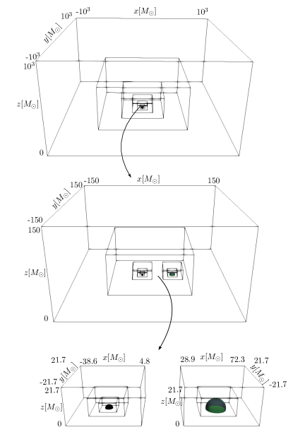
Figure 1: A schematic overview of the grid setup employed in the BAM code. For BHNS systems the BH is resolved with extra refinement levels as compared to the NS. The simulations presented in this article have one additional refinement level for the BH. The finest levels show the BH horizon as ‘black’ contour and the NS as the ‘green’ contour. In all simulations we employ bitant symmetry to save computational costs.

Table 1: Grid configurations. The first column gives the configuration name in the form ‘EOSQmassratio’ where mass ratio is defined as Q$=M^{BH}/M^{NS}_{g}$ and the ‘$\uparrow$’ indicates a (aligned) spinning BH. The next eight columns give the number of levels $L$, the number of moving box levels $L_{\rm mv}$, the number of points in the nonmoving boxes $n$, the number of points in the moving boxes $n_{\rm mv}$, the grid spacing $h_{9}$ ($h_{5}$) in the finest level covering the NS, the grid spacing $h_{10}$ ($h_{6}$) in the finest level covering the BH, the grid spacing $h_{0}$ in the coarsest level, and the outer boundary position $R_{0}$. The grid spacing and the outer boundary position are given in units of $M_{\odot}$.

Name	$L$	$L_{\rm mv}$	$n$	$n_{\rm mv}$	$h_{9}$	$h_{10}$	$h_{0}$	$R_{0}$
EOS1Q2.95	11	3	256	128	0.156	0.078	80.	10240.
EOS3Q2.98	11	3	256	128	0.156	0.078	80.	10240.
SLyQ2	11	3	256	128	0.156	0.078	80.	10240.
SLyQ2↑	11	3	256	128	0.156	0.078	80.	10240.
SLyQ2.84	11	3	256	128	0.156	0.078	80.	10240.
SLyQ2.84↑	11	3	256	128	0.156	0.078	80.	10240.
Poly$\kappa 101.45\Gamma 2$Q2	11	3	256	128	0.188	0.094	96.	12288.
HBQ2-R1	11	3	192	96	0.208	0.104	106.67	10240.
HBQ2-R2	11	3	256	128	0.156	0.078	80.	10240.
HBQ2-R3	11	3	288	144	0.139	0.069	71.11	10240.
Name	$L$	$L_{\rm mv}$	$n$	$n_{\rm mv}$	$h_{5}$	$h_{6}$	$h_{0}$	$R_{0}$
SLyQ4.76	7	4	160	128	0.125	0.063	4.	320.

The computational domain is divided into a hierarchy of cell centered nested Cartesian grids with refinement factor of $2$. The hierarchy consists of $L$ levels of refinement indexed by $l=0,...,L-1$. Each level has one or more Cartesian grids with constant grid spacing $h_{l}$ and $n$ (or $n^{\rm mv}$) points per direction. The grids are properly nested such that the coordinate extent of any grid at level $l,l>0$, is completely covered by the grids at level $l-1$. Refinement levels $l>l^{\rm mv}$ can be dynamically moved and follow the motion of the compact objects according to “moving boxes” technique Brügmann et al. (2008). In this article, we set $l^{\rm mv}=7~{}(2)$. Furthermore, to adequately resolve the BH and the region around it, extra refinement levels can be added only for the BH. In all the simulations presented in this article we add one extra level for the BH. Figure 1 shows a schematic of the refinement grid structure for a typical BHNS simulation in BAM. Moreover, we use bitant symmetry, i.e., reflection across z=0 plane, in the simulations to half the computational costs. In Tab. 1 we list the grid configurations used in this article.

The IDs are evolved with the Z4c formulation of the Einstein equations for the evolution system as described in Sec. (II.1). Constraint damping scheme with values of $\kappa_{1}\in[0.045-0.065]$ and $\kappa_{2}=0$ are used. These values are used based on the suggestions in the detailed 1D numerical analysis of Ref. Weyhausen et al. (2012) and the tests performed in this article, cf. Fig. 2. The combined use of artificial dissipation and constraint damping terms is important (and in some cases essential) to avoid instabilities arising from constraint violating ID inside the BH. BAM  implements a Kreiss-Oliger dissipation of the form 0.5 $\times$ 2^-6 ($\Delta x$)⁶ ($\partial_{x}^{6}+\partial_{y}^{6}+\partial_{z}^{6}$) for all the gravitational field variables at each intermediate Runge–Kutta timestep, where $\Delta x$ is the grid separation Gustafsson et al. (1995).

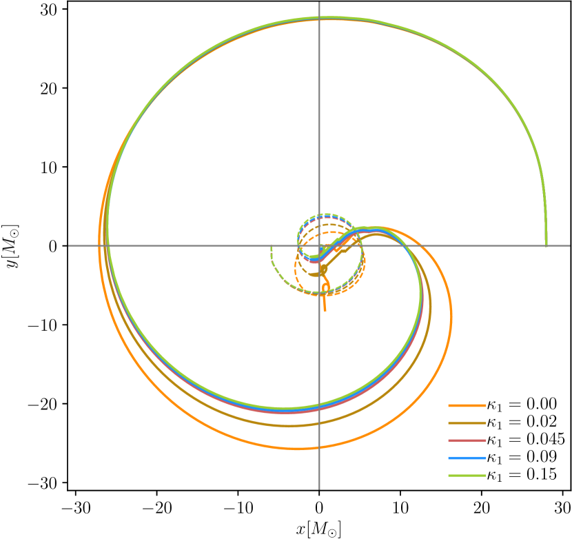
Figure 2: Puncture tracks of the BH (dashed line) and the NS (solid line) for the tests (setup SLyQ4.76) with different constraint damping parameters using the Z4c formulation. Larger values for the $\kappa_{1}$ parameter help in reducing the drift of the center-of-mass that is introduced due to initial constraint violations inside the BH.

We use Sommerfeld boundary conditions Hilditch et al. (2013), the method-of-lines for the time integration with fourth-order Runge-Kutta integrator and fourth-order finite differences for approximating spatial derivatives. A Courant-Friedrich-Lewy (CFL) factor of $0.25$ is employed for all runs Brügmann et al. (2008); Cao et al. (2008). Moreover, the time stepping utilizes the Berger-Collela scheme, enforcing mass conservation across the refinement boundaries Berger and Oliger (1984); Dietrich et al. (2015). GWs are extracted using the curvature scalar $\Psi_{4}$, cf. Sec. III of Brügmann et al. (2008).

The numerical fluxes for the GRHD system, as described in Sec. (II.2), are constructed with a flux-splitting approach based on the local Lax-Friedrich (LLF) scheme. We perform the flux reconstruction with a fifth-order WENOZ algorithm Borges et al. (2008) on the characteristic fields Jiang (1996); Suresh (1997); Mignone et al. (2010) to obtain high-order convergence Bernuzzi and Dietrich (2016). For low density regions and around the moment of merger, we switch to a primitive reconstruction scheme that is more stable but less accurate, i.e., from a scheme with potentially higher order convergence that uses the characteristic fields to a second-order LLF scheme that simply uses, the primitive variables Bernuzzi and Dietrich (2016).

In our simulations the NS is surrounded by an artificial atmosphere, e.g., Thierfelder et al. (2011a); Font et al. (2000); Dimmelmeier et al. (2002). The artificial atmosphere outside of the star is chosen as a fraction of the initial central density of the star as $\rho_{atm}\equiv f_{atm}\cdot\rho_{c}(t=0)$. The atmosphere pressure and internal energy is computed by employing the zero-temperature part of the EOS. The fluid velocity within the atmosphere is set to zero. At the start of the simulation, the atmosphere is added before the first evolution step. During the recovery of the primitive variables from the conservative variables, a point is set to atmosphere if the density is below the threshold $\rho_{thr}\equiv f_{thr}\cdot\rho_{atm}$. In this article, we are using $f_{atm}=10^{-13}$ and $f_{thr}=10^{2}$ in all the configurations.

III.2 Upgrades to simulate BHNS systems

We construct BHNS IDs using the public version of the LORENE code. LORENE employs multi-domain spectral methods to obtain the solution to the elliptic equations Bonazzola et al. (1998); Grandclement et al. (2002). The first BHNS IDs constructed using LORENE are described in Grandclément (2006). Due to the modular architecture of BAM and LORENE, both codes have been easily extended to read and interpolate the spectral ID onto the Cartesian grid of BAM. To import the spectral configurations from LORENE onto our Cartesian simulation grid, we first construct our simulation grid and note the positions of each grid point. Then we evaluate the geometric and the hydrodynamic fields at these positions based on their spectral coefficients. Lastly, the excised BH region is filled with constraint-violating ID, using the “smooth junk” technique Etienne et al. (2007).

As LORENE uses the excision technique for BHs when constructing IDs, the BH interior is removed from the computational domain to avoid pathologies due to the physical singularity and one applies appropriate inner boundary conditions at the excision surface Gourgoulhon et al. (2002); Grandclement et al. (2002). Within BAM, however, we are using the moving puncture approach so that valid data are also required in the excised region of the ID. To circumvent this issue we fill the excised interior with arbitrary but smooth data and evolve it with standard puncture gauge choices as described in Sec. (II.1). During the evolution, we then use the constraint damping properties of the Z4c formulation to reduce effects of the initial constraint violation inside the BH Gundlach et al. (2005); Weyhausen et al. (2012); Cao and Hilditch (2012).

For filling the excised interior, we perform a seventh-order polynomial extrapolation of all the field values radially using uniform points from $r\geq r_{AH}$. The extrapolating polynomial is given explicitly by Lagrange’s formula,

$$f_{n-1}(r_{i})=\sum^{n}_{i=1}L^{n}_{i}(r)f(r_{i})$$ (18)

where $L^{n}_{i}$ is

$$L^{n}_{i}(r)=\prod^{n}_{\begin{subarray}{c}j=1\\ j\neq i\end{subarray}}\frac{r-r_{j}}{r_{i}-r_{j}}.$$

The Lagrange formula is not implemented straightforwardly, but instead via Neville’s algorithm since it is computationally more efficient; the procedure is described in detail in Ref. Press et al. (1992).

IV Code Validation

Table 2: BHNS configurations. The first column refers to the configuration name. The next five columns provide the physical properties of the BH and the NS: the BH area mass $M^{BH}$, the BHs’ dimensionless spin magnitude $\chi^{BH}$ (note we only achieved maximal spins of 0.4 in our tests), baryonic mass of the NS $M^{NS}_{b}$, gravitational mass of the NS $M^{NS}_{g}$ and the NS’s compactness $\mathcal{C}$. The last four columns give the residual eccentricity $e$ in the ID, the initial GW frequency $M\omega^{0}_{22}$, the Arnowitt-Deser-Misner (ADM) mass $M_{\text{ADM}}$, and the ADM angular momentum $J_{\text{ADM}}$. ‘-’ marks the unavailability of eccentricity estimate due to a very short evolution.

Name	$M^{BH}$	$\chi^{BH}$	$M^{NS}_{b}$	$M^{NS}_{g}$	$\mathcal{C}(\frac{M}{R})$	$e$	$M\omega^{0}_{22}$	$M_{\text{ADM}}$	$J_{\text{ADM}}$
SLyQ4.76	6.45	0	1.5	1.354	0.174	-	0.16525	7.7306	28.53
EOS1Q2.95	5	0	1.9	1.694	0.195	0.014	0.05441	6.6413	32.46
EOS3Q2.98	5	0	1.9	1.679	0.202	0.015	0.05424	6.6268	32.19
SLyQ2	2.7	0	1.5	1.354	0.174	0.009	0.05530	4.0169	14.01
SLyQ2↑	2.7	0.4	1.5	1.354	0.174	0.011	0.05517	4.0692	16.86
SLyQ2.84	3.85	0	1.5	1.354	0.174	0.011	0.07754	5.1543	18.61
SLyQ2.84↑	3.85	0.4	1.5	1.354	0.174	0.018	0.07708	5.2283	24.21
Poly$\kappa 101.45\Gamma 2$Q2	2.8	0	1.509	1.403	0.145	0.006	0.03696	4.1728	16.56
HBQ2	2.7	0	1.493	1.350	0.172	0.009	0.05522	4.0129	13.97

To test the validity of our evolution of the filled BHNS system, we perform a comparison with the SXS:BHNS:0002 setup from the SXS collaboration’s BHNS catalog SXS and the setup HBQ2M135 obtained with the SACRA code Kyutoku et al. (2010). Apart from those setups we also evolve other configurations with varying mass ratio, EOS, and spin of the BH. All these setups are tabulated in Tab. 2.

IV.1 Constraints and Mass Conservation

Einstein Constraints:

In Fig. 3 (top and middle panels) we show the evolution of the Hamiltonian and Momentum constraint violations for the HBQ2 setup using different resolutions; cf. Tab. 1 for details. While we find a monotonic decrease of the Hamiltonian constraint for increasing resolution and that the Hamiltonian constraints decrease over time due to constraint damping, the Momentum constraint violations stay at the level of the initial data without noticeable change during the evolution.

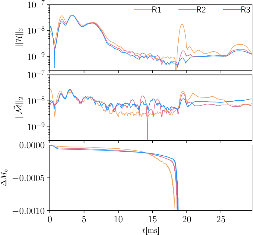
Figure 3: The upper panel shows the $L^{2}$ volume norm of the Hamiltonian constraint, $||\mathcal{H}||_{2}$. The middle panel shows the Euclidean norm of the $L^{2}$ volume norms of the Cartesian components of the momentum constraint, $||\vec{\mathcal{M}}||_{2}=\sqrt{||\mathcal{M}^{x}||^{2}_{2}+||\mathcal{M}^{y}||^{2}_{2}+||\mathcal{M}^{z}||^{2}_{2}}$. The bottom panel shows the evolution of the error in the baryonic mass and stays below 0.01% until the merger. All the quantities here are evaluated on refinement level 3 for HBQ2 setup.

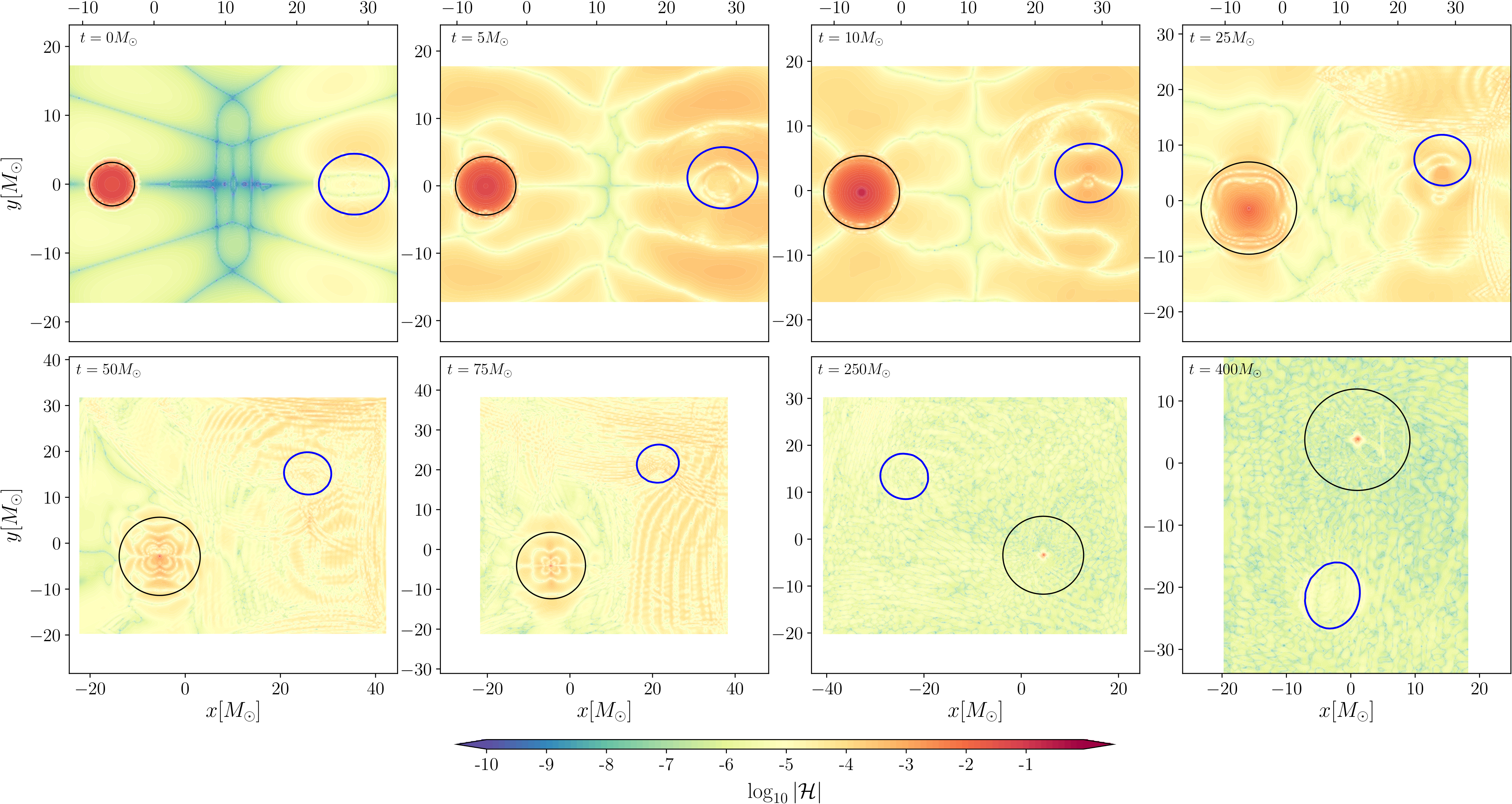
Figure 4: Hamiltonian constraint evolution for the SLyQ4.76 configuration. The black contour marks the apparent horizon of the BH and the blue contour marks the ‘surface’ of the star and corresponds to $\rho=1.462314\times 10^{14}$ g$\cdot$cm^-3. The constraint is computed on the moving level 4 which covers both the compact objects. The apparent horizon radius changes as it is time dependent due to gauge evolution.

For a more detailed understanding about the impact of the BH stuffing and the transition of the early part during the numerical simulation, we present in Fig. 4 the Hamiltonian constraint around the BHNS system at different timesteps for the SLyQ4.76 configuration. As evident from the $t=0$ representation, there are large constraint violations due to the filling of the BH. These constraint violations are within the apparent horizon (marked as black contour). During the course of the evolution, the constraint violation is decreasing inside the BH due to the transition towards the moving puncture gauge. At latest around $\sim 250M_{\odot}$, we find that only the puncture shows large constraint violations.

Considering the evolution of the NS, we find that generally the constraint violation around and inside the NS (blue contour) are not noticeably larger than compared to the surrounding spacetime. Finally, it is worth pointing out that we notice effects of the grid structure of the initial data solver, which is clearly visible in the first two panels, and that we see small reflections of the constraint violation, cf. panel corresponding to $t=75M_{\odot}$.

Overall, while the constraint damping properties of the Z4c evolution scheme lead to a reduction of the constraint violations even within the stuffed BH, we do find that small constraint violations leave the inner part of the BH. Therefore, in contrast to previous works, e.g. Etienne et al. (2009, 2007); Faber et al. (2007), it seems that the exact stuffing and BH filling does have an influence on the dynamical evolution.

Mass Conservation:

The bottom panel of Fig. 3 shows the difference of the baryonic mass during the evolution. Interestingly, we find a small decrease of the baryonic mass during the first few milliseconds of our simulation. This decrease is increasing with resolution and spoils the convergence. After this decrease the mass conservation increases up to the merger of the system when the NS gets disrupted. Because of our particular gauge choice and the usage of an artificial atmosphere, mass is not part of the computational domain once it falls inside the BH Thierfelder et al. (2011b); Dietrich and Brügmann (2014); Dietrich and Bernuzzi (2015).

IV.2 Gravitational-Wave Accuracy

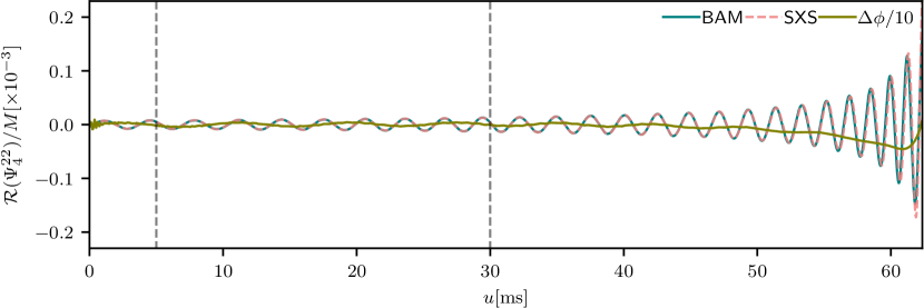
Figure 5: Comparison of $\Psi_{4}^{22}$ from SXS catalog (ID-SXS:BHNS:0002) with BAM’s Poly$\kappa 101.45\Gamma 2$Q2 setup. The alignment interval is marked with vertical dashed lines.

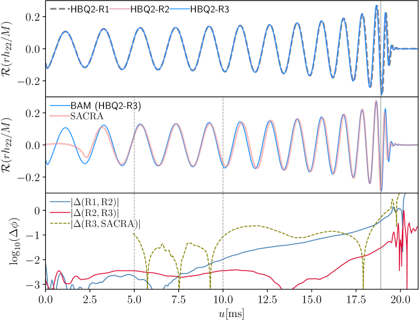
Figure 6: Top: Waveform ($rh_{22}$) comparison among the various BAM resolutions for the HBQ2 configuration. Middle: Comparison of $rh_{22}$ from SACRA (HBQ2M135 Kyutoku et al. (2010)) with BAM’s HBQ2-R3 configuration. Bottom: Phase difference among the various BAM resolutions for the HBQ2 configuration as well as between SACRA and BAM’s HBQ2-R3 configuration. Overall, the phase difference with the SACRA waveform and for the lower BAM resolution (R1-R2) stays $\lesssim 0.5$ rad until the merger whereas for the higher BAM resolution (R2-R3) it stays $\lesssim 0.04$ rad until the merger. The alignment interval is marked with vertical dashed lines and the moment of merger is marked by the solid vertical line.

Figure 5 shows a comparison of the (2,2)-mode of the curvature scalar $\Psi_{4}$ for the BAM evolved Poly$\kappa 101.45\Gamma 2$Q2 setup and the SXS:BHNS:0002 setup from the SXS catalog. Comparing the phase difference between our new BAM simulation and SXS:BHNS:0002, we find phase difference up to the end of the simulation (which corresponds to the merger) of up to $\sim 0.5$ rad.

Figure 6, top panel, shows the comparison of the GW strain $rh_{22}$ from BAM’s HBQ2 simulation for the three employed resolutions R1, R2, and R3. The middle panel shows the comparison of $rh_{22}$ from BAM’s HBQ2-R3 simulation with the HBQ2M135 setup from SACRA. Here the SACRA waveform has been aligned with the BAM waveform in the window marked by vertical dashed-lines as shown in the middle panel of Fig. 6. The bottom panel shows the phase difference for this comparison (olive dashed-line) is $\lesssim 0.5$ rad until the merger. It also shows the phase difference among different BAM resolutions for the HBQ2 configuration. We note that we do not find a clear convergence order for the GW phase, but that, in particular, during the last cycles the phase difference between resolutions R2 and R3 is significantly smaller than between R1 and R2. Furthermore, the overall phase difference is with $\approx 0.5\ \rm{rad}$ for the two lowest resolutions and $\approx 0.04\ \rm rad$ for the two highest resolutions, surprisingly small. Hence, we suggest that there are two possible origins for the missing convergence: (i) The stuffing of the BH at $t=0$ adds a constraint violation that to some extend leave the apparent horizon and effects the overall convergence properties. Such an effect will be investigated through the comparison with another type of initial data that either uses a different stuffing formalism or, ideally, uses puncture initial data as in Refs. Kyutoku et al. (2010). (ii) The phase error is overall smaller than during our previous BNS simulations, which could indicate that the dominant second order error found in previous simulations is absent or suppressed in the case of our BHNS simulations. To investigate this options, we would also need further simulations that go beyond the computational resources available to us for this project.

IV.3 Example Simulations

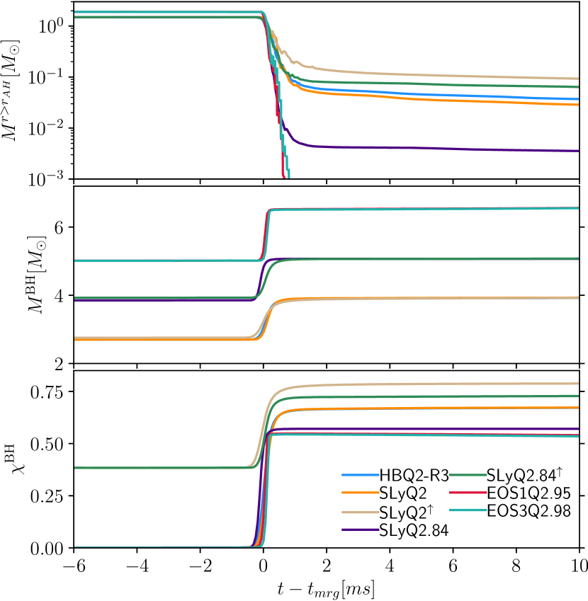
Figure 7: Evolution of the rest mass of the material located outside the apparent horizon (top) , horizon mass (middle) and the dimensionless spin of the BH (bottom) with appropriate time shift; in these plots the time at the onset of the merger is taken as the time origin.

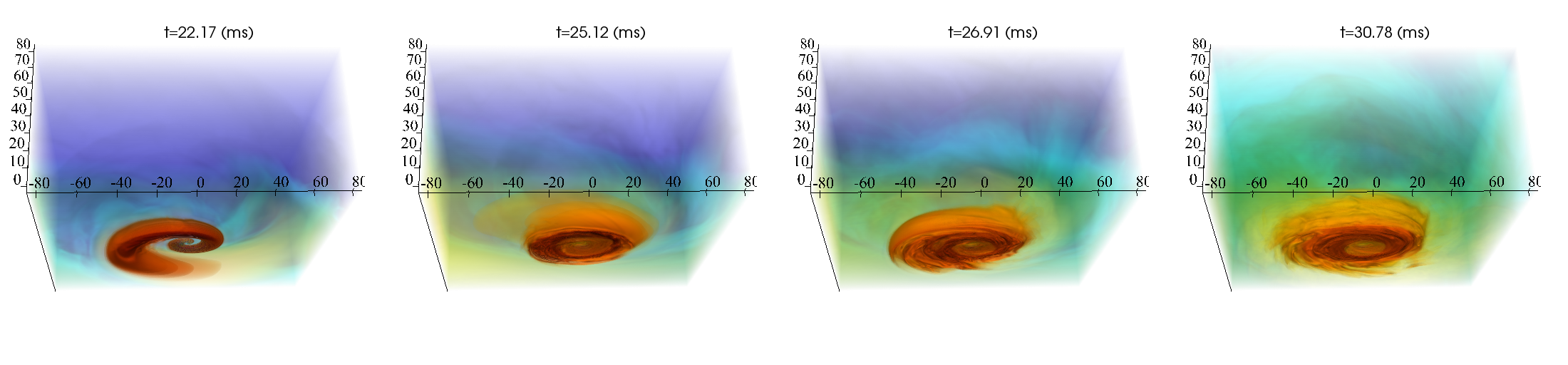
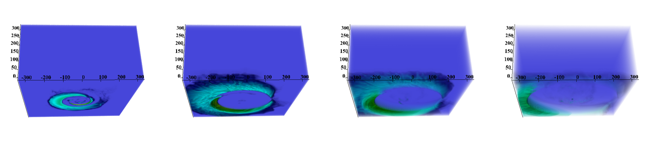
Figure 8: Baryon density ($\rho$) evolution of the bound (Top) and unbound matter (Bottom) for the SLyQ2^↑ configuration at selected timesteps. The 3D-volume consists only of the half-volume that we evolve in the simulations. Specifically, top panel domain consists of $x\in[-80M_{\odot},80M_{\odot}]$, $y\in[-80M_{\odot},80M_{\odot}]$, $z\in[0M_{\odot},80M_{\odot}]$ and bottom panel domain consists of $x\in[-320M_{\odot},320M_{\odot}]$, $y\in[-320M_{\odot},320M_{\odot}]$ and $z\in[0M_{\odot},320M_{\odot}]$. The merger for this setup happens $\sim$ 22 ms.

Table 3: Ejecta and Merger remnants. The first column gives the configuration name and the next five columns list the key quantities: for the ejecta; the unbound mass $M_{\text{ej}}$, its mass-weighted velocity $\bar{v}_{\rm ej}$; and for the merger remnants, the disk-mass $M^{r>r_{\text{AH}}}$, the final BH mass $M^{\text{BH}}$ and its dimensionless spin $\chi^{\text{BH}}$. All the quantities are computed $\sim$ 10 ms after the merger. ‘-’ marks the unavailability of data.

Name	$M_{\text{ej}}$	$\bar{v}_{\rm ej}$	$M^{r>r_{\text{AH}}}$	$M^{\text{BH}}$	$\chi^{\text{BH}}$
	$[10^{-3}M_{\odot}]$	$[c]$	$[M_{\odot}]$	$[M_{\odot}]$
SLyQ4.76	$<$0.1	-	$<$10-5	8.103	0.384
EOS1Q2.95	0.13	0.21	0.0004	6.559	0.540
EOS3Q2.98	0.16	0.24	0.0002	6.553	0.535
SLyQ2	0.37	0.15	0.0286	3.929	0.673
SLyQ2↑	2.45	0.15	0.0927	3.923	0.788
SLyQ2.84	0.30	0.18	0.0035	5.070	0.571
SLyQ2.84↑	5.04	0.22	0.0637	5.075	0.728
HBQ2-R1	0.95	-	0.0427	3.919	0.672
HBQ2-R2	0.59	0.20	0.0382	3.919	0.672
HBQ2-R3	0.44	0.14	0.0369	3.921	0.672

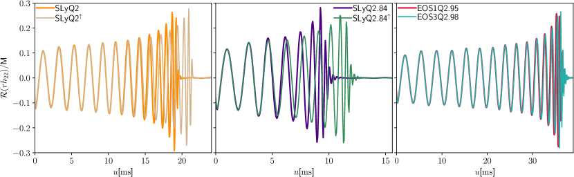
Figure 9: (2,2)-mode of the GW strain $rh_{22}$ for six configurations with varying mass ratio, EOS, and spin of the BH (Tab. 2). GWs are abruptly damped when there is tidal disruption of the NS, e.g., SLyQ2 and SLyQ2^↑ setups whereas BH ringdown is more prominent for high masses ratio cases where the NS is simply swallowed.

We also evolve six additional configurations apart from the three configurations that we use for comparisons and tests. These configurations explore different mass ratios, EOSs, and BH spins (0 and 0.4). The parameters are chosen to favor tidal disruption of the NS (within the possibilities of our ID solver) leading possibly to larger amounts of unbound matter and more massive accretion disks. We would like to note here that the initial residual eccentricities for all the setups evolved in this article are $\mathcal{O}[10^{-3}]$-$\mathcal{O}[10^{-2}]$. The exact values are listed in Tab. 2 and are computed using the trajectories of the compact objects. No eccentricity reduction procedure has been applied to obtain the IDs. Figure 7 shows the evolution of the baryon matter and the BH properties close to the merger and $\sim 10$ms after the merger for all the setups where the postmerger evolution is available. In Tab. 3 we list the disk masses ($M^{r>r_{\text{AH}}}$), the unbound matter ($M_{\text{ej}}$), the mass-weighted ejecta velocity ($\bar{v}_{\rm ej}$), and the postmerger BH properties for the different setups for quantitative comparison, cf. Sec. IIC of Ref. Chaurasia et al. (2018) and references therein for details.

For the highest mass ratio BHNS system (SLyQ4.76) that we simulate the unbound matter and disks are negligible ($<10^{-4}M_{\odot}$ and $<10^{-5}M_{\odot}$, respectively). This is true in general for high mass ratio BHNS systems where the NS is barely subject to any tidal disruption if the companion BH is nonspinning. Lower mass ratio setups lead to disks that increase with decreasing mass ratio. The disk mass is further increased for increasing spin of the BH, i.e., as expected we find aligned spin BH leads to larger disk mass. We find a good agreement between the disk mass as reported for HBQ2M135 (see Ref. Kyutoku et al. (2010), Tab. VIII, $M_{\rm disk}=0.032$) and our HBQ2 setup evolved using BAM. The trend in the ejected mass and its average velocity is more complicated and can vary by 50% among different resolutions. However, a general trend is again that with spin of the BH the amount of unbound matter increases.

The postmerger BH properties for the HBQ2M135 (see Ref. Kyutoku et al. (2010), Tab. VIII, $M_{\rm BH}=3.957M_{\odot}$ and spin $\chi_{\rm BH}=0.67$) are in good agreement with our BAM evolved HBQ2 setup. In high mass ratio mergers, where the compact objects are initially irrotational the final spin of the BH is smaller as compared to lower mass ratio setups or setups where the companion BH is initially spinning. This can be understood as follows: In systems with high mass ratio the NS is not much tidally disrupted and therefore the matter is directly swallowed by the BH. Due to this, the BH is perturbed and undergoes the ringdown phase associated with emission of quasinormal modes. Hence, more GWs are emitted and carry away energy and angular momentum from the system, which leads to a smaller final BH spin. Whereas for lower mass ratios or systems where the BH is spinning, the NS is tidally disrupted leading to an absence of BH ringdown waveforms related to the BH quasinormal modes in the merger and the ringdown phases, cf. Fig. 8. Here the GW amplitude damps abruptly after the inspiral phase when the disrupted material forms a relatively low density and nearly axisymmetric matter distribution around the BH, suppressing GW emission. This leads to the final BH to have larger spins as more angular momentum is available to the system. The waveforms shown in Fig. 9 for the remaining six configurations show the abrupt damping of the GWs for the cases where the NS is tidally disrupted. Furthermore, they follow the expected trends; aligned spin systems SLQ2^↑ and SLyQ3^↑ have a delayed merger as compared to their non-spinning counterparts SLQ2 and SLyQ3 respectively. Overall, the disk mass and postmerger BH property estimates are more robust as compared to the ones for unbound matter.

Finally, Fig. 8 shows the 3D time evolution of the bound (top row) and the unbound (bottom row) matter for the SLQ2^↑ configuration. Due to the comparable masses for a BHNS system (Q$=2$) and the aligned spin of the BH, the NS is tidally disrupted before the merger (first column). This disruption also causes noticeable ejecta that leaves the system. The bound matter then forms a disk surrounding the BH and the unbound matter, mostly expected to be neutron-rich, expands further (second and third columns). In the final stages, the disk still having angular momentum support slowly accretes onto the BH while the ejected matter starts to leave the shown part of the computational domain (fourth columns). Most of the material that is unbound and that will leave the system originates from the tidal tail of the NS due to strong torque. Because of this mechanism, the ejected material is contained within a small azimuthal angle and the ejecta is not distributed axisymmetrically, but as seen in Fig. 8, there is also clear poloidal dependence of the ejected material. Hence, it will be of importance that kilonova models for BHNSs not only incorporate a $\theta$ dependence Kasen et al. (2017); Wollaeger et al. (2018); Perego et al. (2017); Bulla (2019); Kawaguchi et al. (2019); Dietrich et al. (2020); Wollaeger et al. (2021), but also a $\phi$-dependence of the ejecta profiles, e.g., using full 3D profiles from numerical-relativity simulations.

V Summary

In this paper, we presented the first set of BHNS simulations performed with the BAM code. In total, we evolved nine configurations of which we use three for code comparison and tests. We find that BAM evolutions are in good agreement with SACRA simulations, also using the moving puncture gauge, and with excision simulations done with SpEC by the SXS collaboration.

In our simulations, the Z4c scheme with its constraint damping properties has been essential to be able to evolve the stuffed BH. Stuffing was necessary since we used excision ID while the simulations have been performed with the moving puncture gauge. With the Z4c scheme, the overall quality of the simulation seemed good and potentially at the quality that is required for waveform model development. However, we had difficulties in producing adequately convergent initial configurations, hence, a clear quantitative assessment of the numerical uncertainties beyond comparison with previously published data and the simple computation of GW phase differences between different resolutions have not been possible. We suspect this to be caused by excision initial data produced with LORENE. Therefore, we plan more tests with newer solvers like the FUKA solver Papenfort et al. (2021); Fuk in the future. Finally, we find that for the BAM evolved setups the disk mass and the postmerger BH properties are robustly estimated and are consistent with the published literature.

Appendix A GW200115

While this work was being finalized, the announcement of GW200105 and GW200115 Abbott et al. (2021) enhanced further the interest in the simulation of BHNS systems. For this purpose and in preparation of visualizations for public outreach, we have simulated a system consisting of a non-spinning BH with a mass of $6.1M_{\odot}$ and an irrotational NS with a mass of $1.4M_{\odot}$ described by the SLy EOS. These parameters are broadly consistent with the extracted parameters of GW200115. We present snapshots of the simulation in Fig. 10 and refer to a full animation including also the GW signal to the material released during the announcement of GW200115.

As visible in Fig. 10 and in agreement with Ref. Abbott et al. (2021) as well as the non-detection of an electromagnetic signal, e.g., Coughlin et al. (2020); Kasliwal et al. (2020); Anand et al. (2021); Paterson et al. (2021), we find that the NS gets swallowed completely by the BH without being tidally disrupted. Hence, we find no noticeable disk surrounding the final BH ($M_{\rm disk}\lesssim 10^{-5}M_{\odot}$) and no noticeable ejecta material ($M_{\rm ej}\lesssim 5\times 10^{-4}M_{\odot}$).

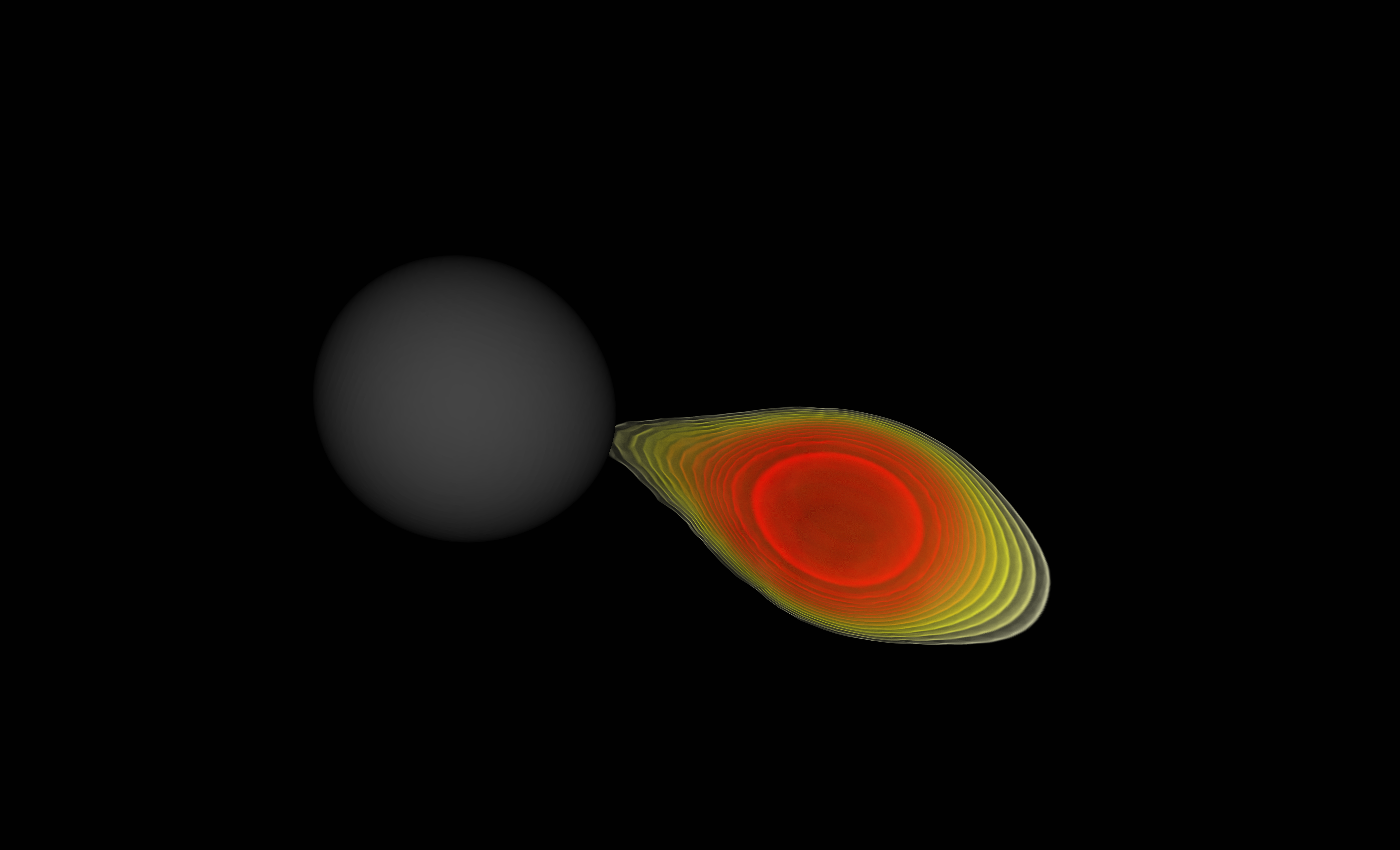
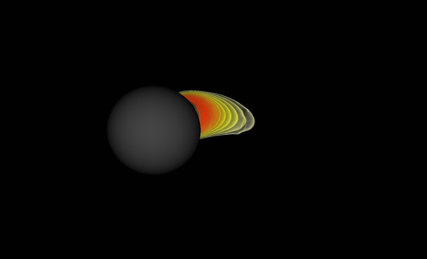
Figure 10: 3D volume rendering of the rest mass density for our GW200115-like system. We visualize the BH as a contour line of the lapse function with $\alpha=0.37$.