UVES analysis of red giants in the bulge globular cluster NGC 6522

Abstract

Context. NGC 6522 is a moderately metal-poor bulge globular cluster ([Fe/H]$\sim$$-$1.0), and it is a well-studied representative among a number of moderately metal-poor blue horizontal branch clusters located in the bulge. The NGC 6522 abundance pattern can give hints on the earliest chemical enrichment in the central Galaxy.

Aims. The aim of this study is to derive abundances of the light elements C and N; alpha elements O, Mg, Si, Ca, and Ti; odd-Z elements Na and Al; neutron-capture elements Y, Zr, Ba, La, and Nd; and the r-process element Eu. We verify if there are first- and second-generation stars: we find clear evidence of Na-Al, Na-N, and Mg-Al correlations, while we cannot identify the Na-O anti-correlation from our data.

Methods. High-resolution spectra of six red giants in the bulge globular cluster NGC 6522 were obtained at the 8m VLT UT2-Kueyen telescope with both the UVES and GIRAFFE spectrographs in FLAMES+UVES configuration. In light of Gaia data, it turned out that two of them are non-members, but these were also analysed. Spectroscopic parameters were derived through the excitation and ionisation equilibrium of Fe I and Fe II lines from UVES spectra. The abundances were obtained with spectrum synthesis. Comparisons of abundances derived from UVES and GIRAFFE spectra were carried out.

Results. The present analysis combined with previous UVES results gives a mean radial velocity of v${}^{\rm hel}_{\rm r}$ = $-$15.62$\pm$7.7 km s^-1 and a metallicity of [Fe/H] = $-$1.05$\pm$0.20 for NGC 6522. Mean abundances of alpha elements for the present four member stars are enhanced with [O/Fe]=+0.38, [Mg/Fe]=$\approx$+0.28, [Si/Fe]$\approx$+0.19, and [Ca/Fe]$\approx$+0.13, together with the iron-peak element [Ti/Fe]$\approx$+0.13, and the r-process element [Eu/Fe]=+0.40. The neutron-capture elements Y, Zr, Ba, and La show enhancements in the +0.08 $<$ [Y/Fe] $<$ +0.90, 0.11 $<$ [Zr/Fe] $<$ +0.50, 0.00 $<$ [Ba/Fe] $<$ +0.63, 0.00 $<$ [La/Fe] $<$ +0.45, and -0.10 $<$ [Nd/Fe] $<$ +0.70 ranges. We also discuss the spread in heavy-element abundances.

1 Introduction

The Galactic bulge formation was probably a result of early mergers and/or dissipative collapse combined with a buckling bar, as suggested by the excellent modern data now available in the innermost parts of the Galaxy (Queiroz et al. 2020a,b, Rojas-Arriagada et al. 2020, Pérez-Villegas et al. 2020, Kunder et al. 2020, Savino et al. 2020 - see also review by Barbuy et al. 2018a), and chemodynamical models (e.g. Fragkoudi et al. 2020, Debattista et al. 2020, Baba & Kawata 2020). Within this context, globular clusters are important tracers of the early formation of the Galactic bulge, assuming that most of them were formed in situ. In particular, their abundance pattern could give hints as to the early nucleosynthesis processes in the Galaxy.

The globular cluster NGC 6522 located in the Galactic bulge was identified by Baade (1946) as having a type II stellar population given its colour-magnitude diagram (CMD); hence, it falling into the Population II class defined in Baade (1944). Despite such an early identification of this cluster, it has not been widely studied since then.

NGC 6522 is an old globular cluster, with a moderate metallicity of [Fe/H]$\sim$$-$1.0, and a blue horizontal branch. Several other such clusters are present in the Galactic bulge, such as NGC 6558 (Rich et al. 1998, Barbuy et al. 2007, 2018b), HP 1 (Barbuy et al. 2006, 2016) , AL 3 (Ortolani et al. 2006), Terzan 9 (Ernandes et al. 2019), and UKS 1 (Fernández-Trincado et al. 2020). Rossi et al. (2015) presented a study gathering these inner globular clusters, that might represent the earliest stellar populations in the Galaxy. Based on their derived proper motions, Rossi et al. (2015) concluded that the inner bulge globular clusters have clearly lower transverse motions and spatial velocities than halo clusters, and they appear to be trapped in the bulge bar.

Pérez-Villegas et al. (2020) computed the orbits of 78 inner Galaxy globular clusters, following the selections given in Bica (2016). It was found that most of the confirmed bulge-population clusters are confined in the bar region but are not supporting the bar structure. For each cluster, a set of 1000 initial conditions were generated, following the Monte Carlo technique and taking into account the observational uncertainties. NGC 6522 has a 99.8% probability of being a bulge member, and most of the orbits among the different initial conditions do support the bar shape. A study of the origin of Galactic globular clusters by Massari et al. (2019) also identified NGC 6522 as having been formed in the main bulge and not, for example, in the Gaia-Enceladus that merged with the Galaxy about 10 Gyr ago. At the same time, it was confirmed to be an old cluster by Kerber et al. (2018): 14.1, 14.2 Gyr for [Fe/H]= $-$1.0, $-$1.15 from BaSTI isochrones (Pietrinferni et al. 2004, 2006) and 12.1, 12.4 Gyr for [Fe/H]=$-$1.0, $-$1.15 from Dartmouth isochrones (Dotter et al. 2008). This old age indicates that NGC 6522 was formed 4 Gyr prior relatively to the estimated age of the bar formation of 8$\pm$2 Gyr by Buck et al. (2018) and $\sim$8 Gyr ago by Bovy et al. (2019). Therefore, the fact that NGC 6522 follows the bar probably indicates that it was confined within the bar when the latter formed.

Barbuy et al. (2009) analysed eight member stars based on FLAMES-GIRAFFE (Pasquini et al. 2002) spectra, included in the survey by Zoccali et al. (2008). Even with these low-resolution spectra (as compared with the UVES spectra analysed later) it was possible to detect some enrichment in s-process elements, which Chiappini et al. (2011a, hereafter C11) interpreted as a possible signature of an early generation of fast rotating stars (the so-called spinstars). This was based on the idea that, as the age-metallicity relation in the bulge was expected to be steeper than in the halo, it would already be possible to reach metallicities as large as [Fe/H] $\sim-$1 on a very short timescale. It was then suggested that in the bulge, globular clusters at [Fe/H] $\sim-$1.0 would already represent tracers of the earliest chemical enrichment phases. Subsequently, we obtained UVES spectra for four of the stars previously analysed in Barbuy et al. (2009) and C11. The re-analysis of these stars based on higher resolution and higher signal-to-noise (S/N) spectra, obtained with the UVES spectrograph at the Very Large Telescope was then presented in Barbuy et al. (2014) where some enrichment of s-process elements in the very old NGC 6522 cluster has been confirmed, although smaller than what was suggested in the earlier low-resolution spectra. It was then necessary to expand the sample to better constrain the nature of the stars that have polluted this very old cluster. With this aim, during our first UVES observations we also obtained parallel observations with the FLAMES-GIRAFFE spectrograph, and new candidate members were identified. These, in turn, were observed with UVES in a new run. In this work, we present results for six stars in NGC 6522 obtained in 2016 with the FLAMES-UVES spectrograph (Dekker et al. 2000). Our main aim is to study the abundance signatures of heavy elements in the cluster.

Furthermore, NGC 6522 was recently shown by Kerber et al. (2018) to have at least two stellar populations in proportions of 86% as second generation (2G) and 14% as first generation (1G). For this reason, we inspected possible Na-O anti-correlations and Na-Al, Na-N, and Mg-Al correlations (Gratton et al. 2012 and references therein) among the present sample stars together with stars analysed in Barbuy et al. (2014).

Finally, we compare element abundance derivation from UVES and GIRAFFE spectra for stars observed with both instruments (in their common wavelength region) to check for further use of the lower resolution spectra. Additionally, in Table 14 in the appendix we list stars identified to be candidate members of the cluster, observed with FLAMES-GIRAFFE, selected from their radial velocities together with Gaia collaboration (2018, 2021) proper motions.

The observations are described in Sect. 2. Photometric stellar parameters’ effective temperature and gravity are derived in Sect. 3. Spectroscopic parameters are derived in Section 4, and abundance ratios are computed in Sect. 5. A discussion is presented in Sect. 6, and conclusions are drawn in Sect. 7.

2 Observations

In Barbuy et al. (2009), eight stars of NGC 6522 observed with the GIRAFFE spectrograph, within the list of over 600 bulge stars analysed by Zoccali et al. (2008) (programs 71.B-0617 and 73.B-0074, PI: A. Renzini) were studied. Four of these were re-observed at higher resolution with UVES and analysed in Barbuy et al. (2014), in programme 88.D-0398 (PI: B. Barbuy) in 2012. From GIRAFFE stars observed in the same field within this same programme, we identified stars with radial velocities and metallicities that could be cluster members. In program 097.D-0175 (PI: B. Barbuy), we observed five of these stars, plus star B118, which was previously studied at a moderate resolution in Barbuy et al. (2009). The log-book of observations is given in Table 1.

The UVES spectra were obtained using the FLAMES setup centred at 580 nm, with a coverage ranging from 480 nm to 680 nm. The 2012 GIRAFFE spectra were obtained using setups HR11 (559.7-584.0 nm) and HR12 (582.1-614.6 nm), and the 2016 GIRAFFE observations used setups HR11, HR13 (612.0-640.5 nm), and HR14A (630.8-670.1 nm), all with a mean resolving power of R $\approx$ 22,000.

The UVES data were reduced with the UVES pipeline v5.7.0 within the REFLEX ambient. The extracted spectra were treated, normalised, rest-frame aligned, and combined using the method described in Section 2.3 of Cantelli (2019). Cosmic-ray removal was done by sigma rejection. Radial velocities were measured using the upper wavelength chip of the UVES red arm, through the IRAF task fxcor, using the Arcturus spectrum as template (Hinkle et al. 2000). The measurements for each star and each exposure and the heliocentric radial velocities computed through the IRAF task rvcorrect are reported in Table 2.

For completeness, and thanks to the Gaia collaboration (2018, 2021) measurements, we were able to proceed to a more robust verification of membership. In Table 3, we list the proper motions ($\mu_{\alpha}\cos\delta$ and $\mu_{\delta}$) and G magnitude from Gaia Early Data Release 3 (EDR3, Gaia Collaboration 2020). With the precision improvement of Gaia EDR3 on proper motions, we recalculated the mean values for NGC 6522. We selected stars within 15 arcmin of the cluster centre and applied the Gaussian mixture models (GMM) to separate the cluster stars from field stars. With this method, we recalculated the cluster proper motion as $\mu_{\alpha}\cos\delta=2.55\pm 0.08$ mas yr^-1 and $\mu_{\delta}=$-$6.45\pm 0.07$ mas yr^-1. Also, the cluster and field distributions allowed us to determine the membership probability for each star. As shown in Table 3, and in the point-vector diagram of Figure 1, stars 234816 and 244523 turn out to be non-members. This shows the power of Gaia, given that these two stars have the very compatible metallicities and radial velocities, coinciding with the other four member stars in the CMD. This is even more striking given that only 0.5% of field stars show a metallicity of [Fe/H]$\mathrel{\hbox{\raise 2.15277pt\hbox{$<$}\hbox to0.0pt{\hss\lower 2.15277pt\hbox{$\sim$}}}}$$-$1.0 in the Galactic bulge (Barbuy et al. 2018a).

A mean heliocentric radial velocity of v${}^{\rm hel}_{\rm r}$ = $-$16.96 km s^-1 is found for the four UVES sample member stars. A mean value of v${}^{\rm hel}_{\rm r}$ = $-$14.3$\pm$3.3 km s^-1 was obtained from UVES spectra of four stars analysed in Barbuy et al. (2014). By combining the present data with these four stars, namely, B-107, B-128, B-122 and B-130, with v${}^{\rm hel}_{\rm r}$ = $-$7.626, $-$14.651, $-$18.043, and $-$16.808 km s^-1, respectively, we obtain a mean value of v${}^{\rm hel}_{\rm r}$ = -15.62 km s^-1. A range of velocities between v${}^{\rm hel}_{\rm r}$ = $-$7.63 and $-$22.57 km s^-1 gives a dispersion of $\pm$7.7 km s^-1. A similar range of radial velocities was detected in Fernández-Trincado et al. (2019), including stars with $-$21.97 $<$ v${}^{\rm hel}_{\rm r}$ $<$ $-$6.61 km s^-1.

The GIRAFFE data were retrieved from the ESO reduced data archive. The extracted spectra belonging to the same setups were then corrected for radial velocity, normalised, and combined by the median. In the appendix, we give a list of new candidate member stars observed with GIRAFFE in 2012 and 2016, within a radial velocity range of $-$14.5$\pm$12 km s^-1, that are confirmed members from proper motions.

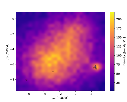
Figure 1: Gaia proper motions at the location of NGC 6522. The background is the proper motion density plot within 8 arcmin of the cluster centre. Blue crosses are the member sample stars, and red crosses are the non-member ones.

Table 1: Log of the spectroscopic observations of programs 088.D-0398(A) and 097.D-0175(A), carried out in 2011-2012 and 2016, respectively. The seeing and airmasses reported are the mean values along the exposures.

Date	UT	Julian	exp	Air-	Seeing
		date	(s)	mass	(′′)
Program 088.D-0398(A)
2011-10-08	00:45:54	2455842.53187	2750	1.462	0.82′′
2011-10-08	01:34:37	2455842.56571	2750	1.853	1.29′′
2012-03-06	07:38:32	2455992.81843	2750	1.579	1.15′′
2012-03-06	08:28:44	2455992.85329	2750	1.260	0.93′′
2012-03-07	07:47:56	2455993.82495	2750	1.489	0.81′′
2012-03-07	08:39:16	2455993.86060	2750	1.270	0.73′′
2012-03-25	08:31:47	2456011.85541	2750	1.087	0.64′′
Program 097.D-0175(A)
2016-05-17	07:22:18	2457525.80716	2400	1.007	0.40′′
2016-05-17	08:05:08	2457525.83690	2400	1.033	0.47′′
2016-05-17	08:52:35	2457525.86985	2400	1.099	0.47′′
2016-07-11	02:33:35	2457580.60666	2400	1.028	0.96′′
2016-07-21	03:27:16	2457590.64394	2400	1.016	0.51′′
2016-07-21	04:43:37	2457590.69696	2400	1.112	0.54′′
2016-07-21	06:33:32	2457590.75246	2400	1.373	0.54′′
2016-07-22	04:48:26	2457591.70031	2400	1.131	0.48′′
2016-07-22	05:40:15	2457591.73629	2400	1.288	0.45′′
2016-07-22	06:33:29	2457591.77326	2400	1.574	0.63′′

Table 2: Observed and heliocentric radial velocities of the UVES sample stars, in each of the 10 UVES exposures, and the mean heliocentric radial velocity.

OGLE n∘		234816		244523		244819		256289		B118		402370
Date	UT	Observed and Heliocentric radial velocity (${\rm km.s^{-1}}$)
		vobs	vhel	vobs	vhel	vobs	vhel	vobs	vhel	vobs	vhel	vobs	vhel
17-05-2016	07:22:18.596	$-$31.90	$-$15.21	$-$29.59	$-$12.89	$-$39.18	$-$22.49	$-$31.56	$-$14.87	$-$36.48	$-$19.79	$-$27.20	$-$10.51
17-05-2016	08:05:08.353	$-$31.98	$-$15.36	$-$29.66	$-$13.95	—	—	$-$31.75	$-$15.13	$-$36.61	$-$19.99	$-$27.53	$-$10.92
17-05-2016	08:52:35.292	$-$31.67	$-$15.13	$-$29.39	$-$12.85	$-$39.15	$-$22.61	$-$31.17	$-$14.63	$-$36.36	$-$19.82	$-$27.20	$-$10.66
11-07-2016	02:33:35.361	$-$06.85	$-$15.93	$-$04.61	$-$13.68	$-$13.99	$-$23.07	$-$06.42	$-$15.49	$-$10.98	$-$20.05	$-$02.02	$-$11.09
21-07-2016	03:27:16.562	$-$01.53	$-$15.27	0.76	$-$12.99	$-$08.47	$-$22.22	01.48	$-$12.27	$-$05.48	$-$19.22	02.69	$-$11.06
21-07-2016	04:43:37.414	$-$01.36	$-$15.24	0.77	$-$13.11	$-$08.14	$-$22.03	$-$0.92	$-$14.80	$-$05.25	$-$19.13	02.70	$-$11.19
21-07-2016	06:33:32.375	$-$1.33	$-$15.33	0.55	$-$13.46	$-$8.21	$-$22.21	$-$0.81	$-$14.82	$-$5.11	$-$19.11	2.84	$-$11.18
22-07-2016	04:48:26.611	$-$01.04	$-$15.37	01.11	$-$13.22	$-$08.38	$-$22.71	$-$0.54	$-$14.87	$-$05.36	$-$19.69	03.78	$-$10.55
22-07-2016	05:40:15.273	$-$01.39	$-$15.80	0.26	$-$14.15	$-$08.26	$-$22.67	$-$0.79	$-$15.20	$-$5.18	$-$19.59	02.89	$-$11.52
22-07-2016	06:33:29.572	$-$0.88	$-$15.36	1.11	$-$13.37	$-$08.66	$-$23.14	$-$0.44	$-$14.92	$-$05.12	$-$19.60	3.48	$-$11.00
Mean vhel			$-$15.40		$-$13.37		$-$22.57		$-$14.70		$-$19.60		$-$10.97

Table 3: Identifications and Gaia proper motions; Gaia G and Johnson B and V magnitudes and membership probability. Stars from Barbuy et al. (2009, 2014) are also included.

OGLE	Name	pmRA	pmDEC	$Gmag$	$V$	$B$	$\mathcal{P}_{Member}$
	Present work
234816		$-6.1170$	$-8.3550$	$15.6950$	$16.401$	$17.781$	0
244523		$-3.0400$	$-6.9400$	$15.3813$	$15.988$	$17.283$	0
244819		$2.6380$	$-6.6090$	$15.6814$	$16.306$	$17.614$	100
256289		$2.5830$	$-7.1310$	$15.3887$	$15.918$	$17.192$	98
402322	B118	$2.4800$	$-6.5720$	$15.3817$	$16.011$	$17.331$	100
402370		$2.4900$	$-6.6590$	$15.5926$	$16.226$	$17.551$	100
Stars from Barbuy et al. (2014)
402361	B107	$2.8460$	$-6.8850$	$15.3375$	$15.980$	$17.292$	100
244582	B122	$2.4820$	$-6.0110$	$15.3401$	$16.000$	$17.354$	99
402607	B128	$2.4810$	$-6.4190$	$15.6001$	$16.260$	$17.621$	100
402531	B130	$3.0100$	$-6.1770$	$15.6871$	$16.300$	$17.597$	100
	Other stars from Barbuy et al. (2009)
412752	B008	$2.6170$	$-6.4500$	$15.4115$	$15.990$	$17.402$	100
–	B108	$3.3340$	$-6.2990$	$15.1898$	$16.290$	$18.313$	99
–	B134	$0.7350$	$-5.0020$	$15.5082$	$16.040$	$17.367$	0
244829	F121	$2.2580$	$-7.0090$	$15.7923$	$16.400$	$17.849$	99

3 Photometric stellar parameters

3.1 Temperatures

The selected stars, their OGLE and 2MASS designations, coordinates, and $VIJHK_{\rm s}$ magnitudes are given in Table 4. $V$ and $I$ data were collected from the Optical Gravitational Lensing Experiment (OGLE) survey, the OGLE-II release, Field Bul-SC45 centered at 18:03:33.0, $-$30:05:00 from Udalski et al. (2002). 2MASS $J$, $H$, and $K_{\rm s}$ are from Skrutskie et al. (2006), and VVV $J$, $H$, and $K_{\rm s}$ magnitudes are from the Vista Variables in the Via Lactea survey (Saito et al. 2012). Table 3 reports the Gaia (2018, 2020) G magnitudes and deduced B magnitudes by applying the transformation $G_{\rm mag}-V_{C}=f(B-V)$ from Riello et al. (2021). In Fig. 2, we show the location in $B$, $V$ of the sample stars, in the CMD of NGC 6522 from data observed in F435W and F555W with the Hubble Space Telescope, and converted to $B$ and $V$ by Piotto et al. (2002).

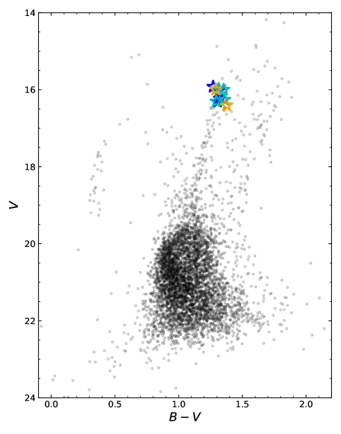
Figure 2: NGC 6522 Colour-magnitude diagram $V$ versus $B-V$ by Piotto et al. (2002) with the location of the observed stars. Present four stars: blue. Four stars from Barbuy et al. (2014): cyan. Two non-member stars: orange.

Photometric effective temperatures and bolometric corrections were derived from $V-I$, $V-K$, and $J-K$ using the colour-temperature calibrations of Alonso et al. (1999, hereafter AAM99) and Casagrande et al. (2010, hereafter C10). For the transformation of $V-I$ from the Cousins to Johnson system, we used ($V-I$)_C=0.778($V-I$)_J (Bessell 1979). $J$,$H$, and $K_{S}$ 2MASS magnitudes and colours were transformed from the 2MASS system to the California Institute of Technology (CIT), and from this to TCS (Telescopio Carlos Sánchez), following Carpenter (2001) and Alonso et al. (1998). The VVV $JHK_{s}$ colours were transformed to the 2MASS $JHK_{s}$ system using relations by Soto et al. (2013) and then transformed to CIT as above.

The derived photometric effective temperatures, which are adopted as initial guesses, resulting from relations from AAM99 and C10 are both listed in Table 5. The differences in effective temperatures, in the $\Delta$T_eff(C10-AAM99) sense, are of +64.7 K, +54.2 K and $\pm$140 K for $V-I$, $V-K$ and $J-K,$ respectively. These temperatures are used only as a guide to start fitting them from the Fe I and Fe II lines.

3.2 Gravities

For a derivation of photometric gravities, we used the classical formula, adopting T_eff,⊙=5770 K, M_∗=0.85 M_⊙, and M_bol,⊙ = 4.75. For the cluster, we used a distance modulus of ($m-$M)₀ = 14.40 and a reddening of E(B-V)=0.52 and A_V = 1.61, based on Kerber et al. (2018). Bolometric corrections were derived using AAM99 and C10 assuming BC${}_{\rm V,\odot}=$-$0.07$, M${}_{\rm V,\odot}=4.81$, and M${}_{\rm I,\odot}=4.10$ from Willmer (2018). The computed bolometric magnitudes and gravities are given in Table 5.

Table 4: Identifications, coordinates, and magnitudes. $JHK_{s}$ from both 2MASS and VVV surveys.

OGLE	---2MASS ID	$\alpha_{2000}$	---$\delta_{2000}$	---$V$	---$I$	---$J$	---$H$	---$K_{\rm s}$	---$J_{\rm VVV}$	---$H_{\rm VVV}$	$K_{\rm VVV}$
234816	18032652-3006385	18:03:26.52	$-$30:06:38.1	16.401	14.604	13.198	12.488	12.302	13.1735	12.5075	12.3052
244523	18032757-3003455	18:03:27.56	$-$30:03:45.1	15.988	14.325	12.667	11.872	12.274	13.0323	12.4093	12.233
244819	18033354-3002254	18:03:33.51	$-$30:02:25.2	16.306	14.672	13.020	12.284	11.421	13.3148	12.6694	12.499
256289	—	18:03:31.58	$-$30:00:51.0	15.918	14.337	—	—	—	13.0892	12.4721	12.289
402322	18034225-3003403	18:03:42.25	$-$30:03:40.0	16.011	14.313	13.056	12.305	12.142	12.9661	12.324
402370	18034235-3002088	18:03:42.35	$-$30:02:08.5	16.226	14.554	13.391	12.673	12.550	13.2643	12.628

Table 5: Photometric stellar parameters derived using the calibrations by Alonso et al. (1999) (AAM99) and Casagrande et al. (2010) (C10) for $V-I$, $V-K$, $J-K$, bolometric corrections, bolometric magnitudes and corresponding gravity log $g$.

star	T($V-I$)	T($V-K$)	T($J-K$)	T($V-K$)	T($J-K$)	log(Teff)	${\rm BC_{V}}$	${\rm M_{bol}}$	log g	Calib
		2MASS	2MASS	VVV	VVV	(mean)
	(K)	(K)	(K)	(K)	(K)
234816	$4517.1$	$4504.8$	$4693.7$	$4501.0$	$4579.4$	$3.655$	$-0.475$	$0.86$	$2.363$	AAM99
	$4600.0$	$4568.4$	$4843.0$	$4564.5$	$4712.6$	$3.668$	$-0.477$	$0.86$	$2.414$	C10
244523	$4792.5$	$4848.0$	$7391.8$	$4799.3$	$4806.5$	$3.681$	$-0.344$	$0.32$	$2.249$	AAM99
	$4854.4$	$4912.6$	$7372.1$	$4865.1$	$4969.3$	$3.732$	$-0.351$	$0.32$	$2.453$	C10
244819	$4858.8$	$4027.3$	$3340.5$	$4749.2$	$4746.3$	$3.687$	$-0.319$	$0.62$	$2.391$	AAM99
	$4917.7$	$4039.6$	$3115.6$	$4815.7$	$4902.1$	$3.639$	$-0.325$	$0.61$	$2.199$	C10
256289	$4986.7$	—	—	$4928.7$	$4805.2$	$3.698$	$-0.277$	$0.19$	$2.264$	AAM99
	$5042.1$	—	—	$4990.7$	$4967.9$	$3.699$	$-0.279$	$0.18$	$2.264$	C10
402322	$4715.8$	$4698.8$	$4638.5$	$4681.9$	$4686.9$	$3.674$	$-0.376$	$0.37$	$2.242$	AAM99
	$4782.2$	$4765.6$	$4780.3$	$4748.8$	$4835.3$	$3.680$	$-0.383$	$0.37$	$2.266$	C10
402370	$4772.5$	$4887.1$	$4873.3$	$4786.4$	$4778.9$	$3.679$	$-0.352$	$0.57$	$2.341$	AAM99
	$4835.4$	$4950.6$	$5043.1$	$4852.4$	$4938.6$	$3.692$	$-0.359$	$0.56$	$2.393$	C10

Table 6: Final UVES spectroscopic parameters.

star	-Teff	-log g	-[FeI/H]	-[FeII/H]	-[Fe/H]	${\rm v_{t}}$
	(K)					km s-1
234816	4650	2.25	$-$1.03	$-$1.08	$-$1.05	1.65
244523	4800	2.00	$-$1.10	$-$1.12	$-$1.11	2.30
244819	4690	2.30	$-$1.23	$-$1.19	$-$1.21	1.51
256289	4770	2.10	$-$1.12	$-$1.11	$-$1.11	1.25
B118	4820	2.20	$-$1.18	$-$1.16	$-$1.17	2.10
402370	4700	2.20	$-$1.15	$-$1.16	$-$1.15	1.15

4 Spectroscopic stellar parameters

The equivalent widths (EW) of Fe I and Fe II lines were measured using IRAF. The EWs, together with wavelength (Å); excitation potential (eV), damping constant C₆ and oscillator strengths from VALD3 (Piskunov et al. 1995, Ryabchikova et al. 2015), National Institute of Standards & Technology (NIST, Martin et al. 2002) and Kurúcz (1993), and adopted values are given in Table C. For Fe I, we chose NIST values when available, otherwise they are from VALD3. In most cases, these coincide with the value from Kurucz, as can be seen in Table C. For Fe II, values from Meléndez & Barbuy (2009) are used. The solar abundances were adopted from Grevesse & Sauval (1998), including $\epsilon$(Fe)=7.50 for Fe, except for A(O)=8.76 for oxygen from Steffen et al. (2015).

The models were interpolated in the MARCS model atmospheres grid (Gustafsson et al. 2008). We adopted the spherical and mildly CN-cycled set ([C/Fe]$=-0.13$, [N/Fe]$=+0.31$). These models consider [$\alpha$/Fe]=+0.20 for [Fe/H]=-0.50 and [$\alpha$/Fe]=+0.40 for [Fe/H]$\leq-$1.00. The LTE abundance analysis and the spectrum synthesis calculations were performed using the code described in Barbuy et al. (2018c). The code is an update of the Meudon ABON2 code by M. Spite, continously improved along the years, which adopts local thermodynamic equilibrium (LTE). In Trevisan et al. (2011), the calculation of lines and in particular the continuum opacity calculation were cross-checked with the code by the Uppsala group BSYN/EQWI (Edvardsson et al. 1993, and updates until that date). The basic atomic line list is from VALD3 (Ryabchikova et al. 2015). Molecular lines of CN (A²$\Pi$-X²$\Sigma$), C₂ Swan (A³$\Pi$-X³$\Pi$), TiO (A³$\Phi$-X³$\Delta$) $\gamma$, TiO (B³$\Pi$-X³$\Delta$) $\gamma$’, TiO $\alpha$ C³$\Delta-$X³$\Delta,$ and TiO $\beta$ c¹$\Phi-$a¹$\Pi$ systems are taken into account, as described in Barbuy et al. (2018c).

We initially adopted the photometric effective temperature and gravity, and then further constrained the temperature by imposing an excitation equilibrium for Fe I lines and gravities by imposing ionisation equilibrium from lines of Fe I and Fe II. Microturbulence velocities v_t (km s^-1) were determined by cancelling the trend of Fe I abundance versus EW. Fits to the observed spectra in regions containing the Fe II lines were carried out, as shown in Fig. 3 for star 256289. The good match of the Fe II lines indicates that these lines correspond to the equivalent widths measured, that they are not plagued by blends, and that the stellar parameters are suitable. The final spectroscopic parameters T_eff, log g, [Fe I/H], [Fe II/H], [Fe/H] and v_t values are reported in Table 6. An example of excitation and ionisation equilibrium using Fe I and Fe II lines is shown in Fig. 4 for star B118.

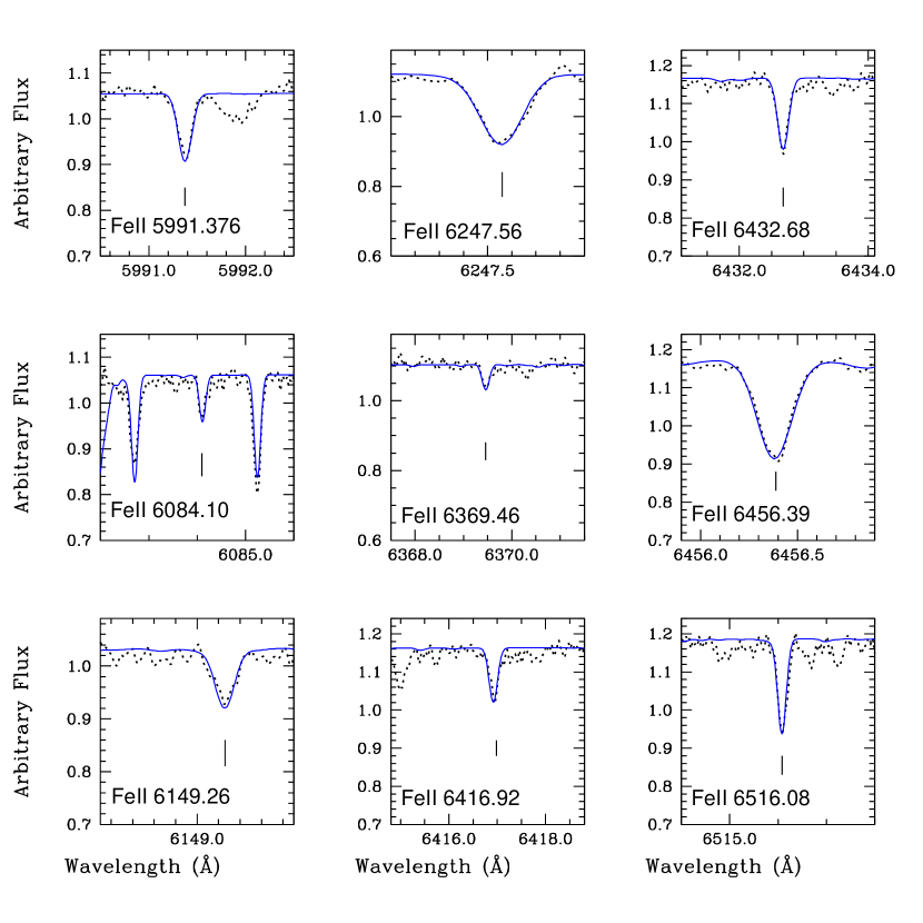
Figure 3: Fe II lines in star 256289.

Figure 4: Excitation and ionisation equilibrium in star B118.

5 Abundance ratios

Abundances ratios were obtained by means of line-by-line spectrum synthesis calculations compared to the observed spectra. The abundance derivation details are explained below, and the results are reported in Table 7 for C, N, and O; and Table 8 for the $\alpha$-elements O, Mg, Si, Ca, Ti, odd-Z elements Na, Al, and heavy elements Y, Zr, Ba, La, Nd, and Eu.

5.1 Carbon, nitrogen, and oxygen

Table 7: Carbon, nitrogen, and oxygen abundances derived from C₂ (0,1), CN (5,1), and [OI] lines.

line	---$\lambda$(Å)	--234816	--244523	--244819	--256289	--B118	--402370
C2(0,1)	-5635.5	-$\leq$+0.0	-$\leq$+0.2	-$\leq$+0.2	-$\leq$+0.2	-$\sim$+0.2	-$\leq$+0.0
CN(5,1)	-6332.2	-$\leq$+0.8	-$\leq$+0.8	-$\leq$+1.2	-$\leq$+0.3	-$\leq$+0.8	-$\leq$+0.3
[OI]	-6300.3	+0.60	+0.40	+0.40	+0.40	—	+0.40

Table 7 gives the results for C, N, and O abundances. The carbon abundances were estimated from the molecular C₂(0,1) Swan bandhead at 5635.5 Å. These bandheads are faint, and in these stars they allow us to give an upper limit only. The atomic C I 5380.3 Å lines are essentially absent in these stars and cannot be used. The nitrogen abundance is derived from the CN(5,1) red system bandhead at 6332.2 Å. For the oxygen-forbidden line at [OI] 6300.311 Å, a selection among the original spectra where telluric lines did not contaminate the line was needed, since most of the observations were contaminated. A few spectra were retrieved showing a clean [OI] 6300.311 Å line, and the oxygen abundance was derived. Figure 5 shows fits to C₂, CN and [OI] lines for star 244819.

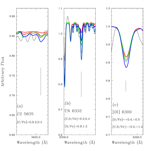
Figure 5: C, N, and O lines in star 244819: Panel (a): C₂ 5635 Å computed with ([C/Fe], [N/Fe], [O/Fe]) = (0.0, 0.8, 0.4), (0.2, 0.8, 0.4) in red, (0.2, 1.2, 0.4) in green, (0.4, 1.2, 0.4) in blue. Panel (b): CN 6332 Å computed with: (0.2, 0.8, 0.4) in red, (0.2, 1.2, 0.4) in green, (0.4, 0.8, 0.4) and (0.4, 1.2, 0.4) in blue. Panel (c): [OI] 6300 Å computed with (0.2, 0.8, 0.4) in red, (0.2, 1.2, 0.4) in green, (0.2, 1.2, 0.5) in blue. In all cases, black dotted lines are the observed spectra.

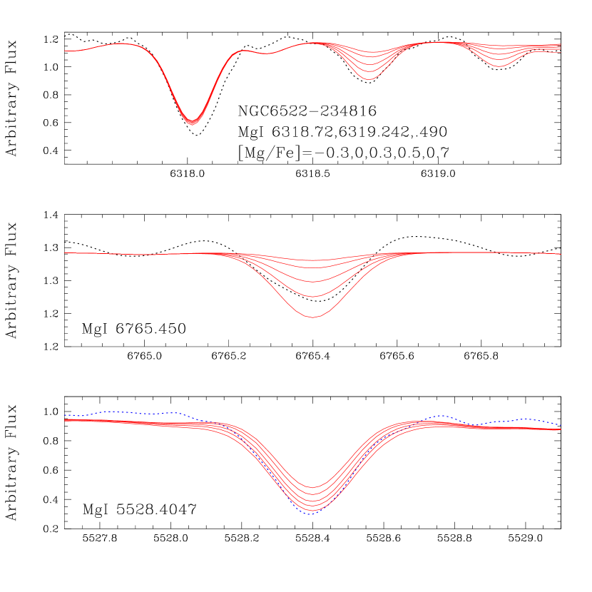
Figure 6: Fits to Mg I lines in star 234816.

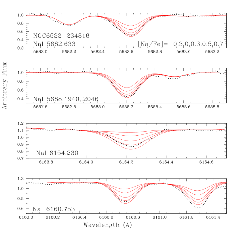
Figure 7: Fits to Na I lines in star 234816.

5.2 Odd-Z and alpha elements

Line-by-line abundances of the odd-Z elements Na and Al and alpha elements Mg, Si, Ca, and Ti are reported in Table 8. Ti is an iron-peak element, but given its behaviour following the alpha-elements, it is often considered as an alpha.

For star 234816, there is a clear overenhancement of the alpha elements as well as of the r element Eu. Figure 6 shows the MgI lines studied showing agreement for a high enhancement of [Mg/Fe]=+0.7. The odd-Z elements Na and Al are also enhanced in this star, with [Na/Fe]=[Al/Fe]=+0.5, as illustrated for Na lines in Figure 7.

We exhaustively remeasured equivalent widths using other tools than IRAF, and we redetermined stellar parameters, and even with somewhat different stellar parameters. Models of (T_eff, log g, [Fe/H], v_t) = (4530 K, 2.2, $-$1.04, 1.2 km.s^-1) and (4440 K , 2.02, $-$0.78, 1.11 km.s^-1) were employed in Cantelli (2019), and the overenhancement in alpha elements persists.

5.3 Heavy elements

Line-by-line abundances of Y, Zr, Ba, La, Nd, and Eu are reported in Table 8. In Table 9 the mean abundances are reported, including results from Barbuy et al. (2014). Below we describe details on the lines of the heavy elements studied.

Barium, Lanthanum and Europium: The hyperfine structure (HFS) for the studied lines of Ba II 5853.675, 6141.713 and 6496.897 Å and Eu II 6645.064 Å were taken into account. For Ba II 5853.675, we computed the splitting of lines by employing a code made available by Andrew McWilliam (McWilliam et al. 2013). For Ba II 6141.713 Å and Ba II 6496.897 Å lines, as well as for La II lines, the HFS structure was reported in Barbuy et al. (2014), and for Eu II 6645.064 Å the HFS was adopted from Hill et al. (2002). For Ba II 5853.675 Å, the magnetic dipole A-factor, and the electric quadrupole B-factor were adopted from Biehl (1976) and Rutten (1978), as given in Table 15. The nuclear spin is I=1.5 and the isotopic nuclides Ba¹³⁸ and Ba¹³⁷ Ba¹³⁶, Ba¹³⁵ and Ba¹³⁴ contribute with 71.7% and 11.23%, 7.85%, 6.59%, 2.42%, respectively (Asplund et al. 2009). The hyperfine splitting applies only to the odd-Z nuclides Ba¹³⁵ and Ba¹³⁷. The line list taking into account hyperfine structure for Ba II 5853.675 Å is given in Table 16.

Figures 8, 9, 10, 11, and 12 show, respectively, the fits to the Y I and Y II, three Ba II, La II, Nd II lines, and Eu II studied lines in the six sample stars.

Strontium: We carefully inspected the Sr lines and give the conclusions here. The line Sr I 6503.989 Å is in the wing of another line and is very shallow; Sr I 6791.016 Å is also very shallow, and only at higher S/N it could be used (as we did in Barbuy et al. 2014). We here describe the blends contained in the Sr I 6550.244 Å line in detail. In Figure 13, we show that: a) despite the presence of several TiO lines from the $\gamma$, $\gamma$’, $\alpha,$ and $\beta$ systems, they are faint, given that TiO only gets stronger is very cool stars. To take the TiO lines into account, we adopted [O/Fe], [Ti/Fe] from Table 9; b) There are lines of Mn II, Cr I, Ca I, Fe II, Sc II, Ni I, Si I, and Tm II, but all of these are extremely faint and do not influence the strength of the blend; c) The Nd II 6550.178 Å line is not very strong, but it does contribute to the strength of the blend. We used three Nd II lines to derive [Nd/Fe] for the sample stars, and the fits are presented in Fig. 11. The resulting mean Nd abundance is then fixed in order to compute the Sr abundance. In Fig. 13, we show the Nd line for the abundance derived and also for a +0.1 or +0.2dex increase; d) The main contributors to a blend are C₂ and CN lines. Although the C and N abundances are upper limits, by adopting these values the blend is strong. The computations were done for [C/Fe]=0.2 and [N/Fe]=0.8 (that are the upper limits given in Table 5). Since C and N are anticorrelated we compute also with [C/Fe]=0.1 and [N/Fe]=0.9 and [C/Fe]=0.3 and [N/Fe]=0.7: the strong variation in the C₂ and CN line strengths make the derivation of Sr abundance very uncertain. The identified lines are C₂ Swan system (v’,v”) = (2,5): R3(30) 6550.660, R2(31) 6550.398 and R1(32) 6550.296 and CN red system (v’,v”) = (6,2): Q1(22) 6550.269 Å; e) In conclusion, we estimate values of [Sr/Fe]=+1.6 for star 244816 and [Sr/Fe]=+0.7 for star B118 but these cannot be considered reliable.

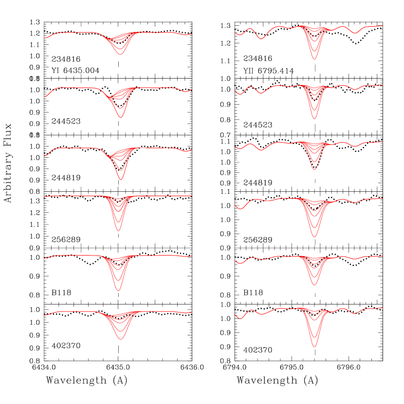
Figure 8: Fits to Y I 6435.004, and Y II 6795.414 Å in the six sample stars. Observed spectra (black dotted lines) are compared with synthetic spectra (red lines) computed for [Y/Fe]=$-$0.3,0,0.3,0.5,0.8,1.0.

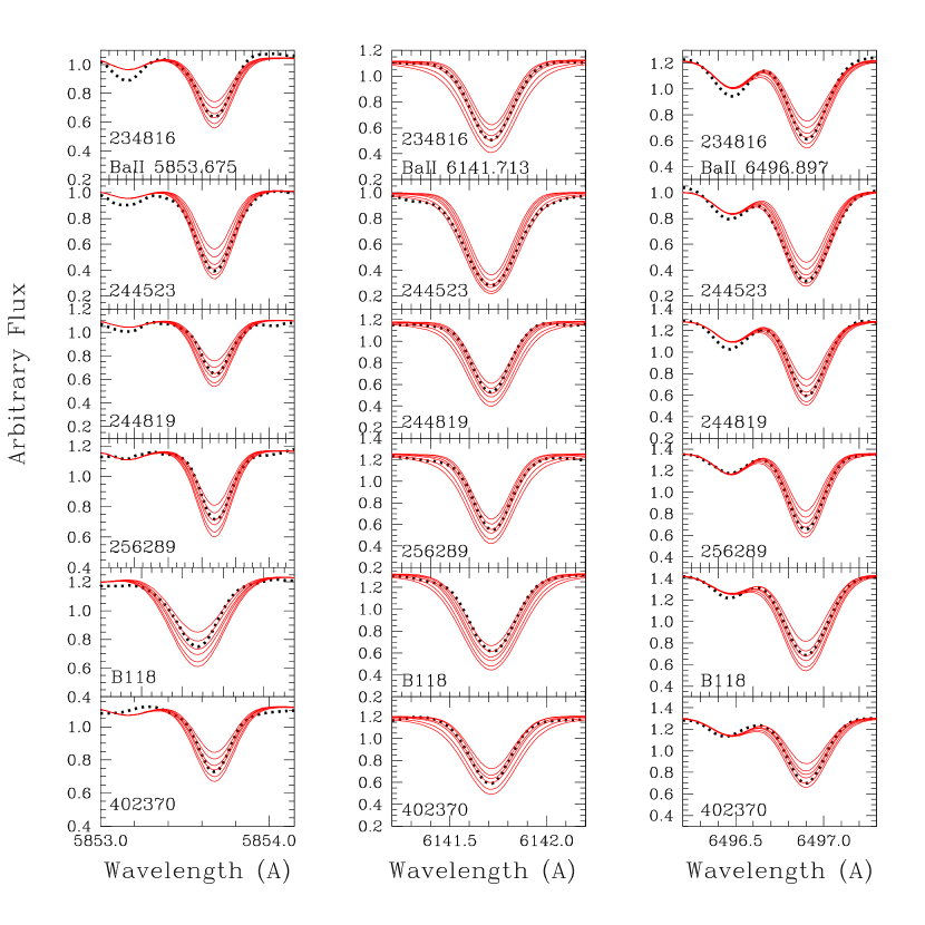
Figure 9: Fits to Ba II 5853.675, 6141.713 and 6496.897 Å in the six sample stars. Observed spectra (black dotted lines) are compared with synthetic spectra (red lines) computed for [Ba/Fe]=$-$0.3,0,0.3,0.5,0.8,1.0.

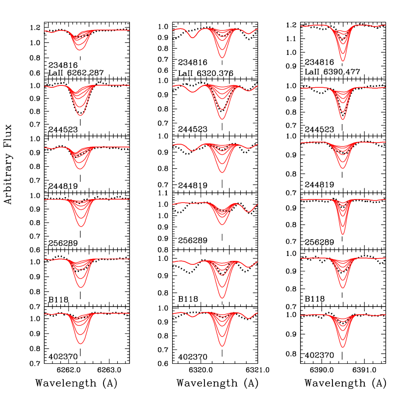
Figure 10: Fits to La II 6262.287, 6320.376, and 6390.477 Å in the six sample stars. Observed spectra (black dotted lines) are compared with synthetic spectra (red lines) computed for [La/Fe]=$-$0.3,0,0.3,0.5,0.8,1.0.

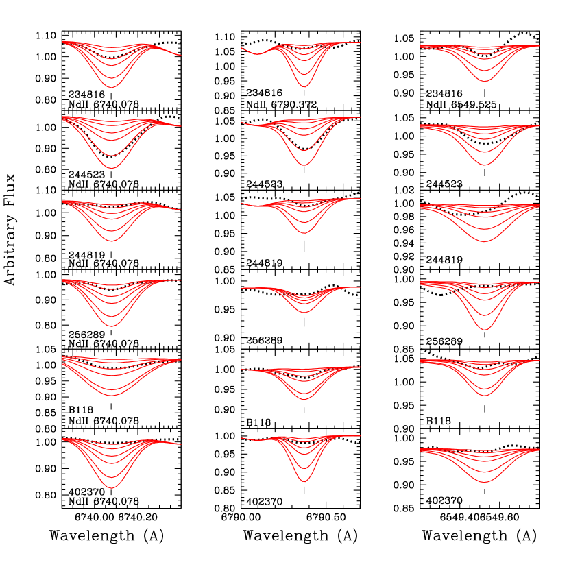
Figure 11: Fits to Nd II 6740.078, 6790.372 and 6549.525 Å in the six sample stars. Observed spectra (black dotted lines) are compared with synthetic spectra (red lines) computed for [Nd/Fe]=$-$0.3,0,0.3,0.5,0.8,1.0.

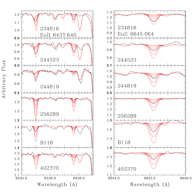
Figure 12: Fits to Eu II 6437.650 and 6645.064 Å in the six sample stars. Observed spectra (black dotted lines) are compared with synthetic spectra (red lines) computed for [Eu/Fe]=$-$0.3,0,0.3,0.5,0.8,1.0.

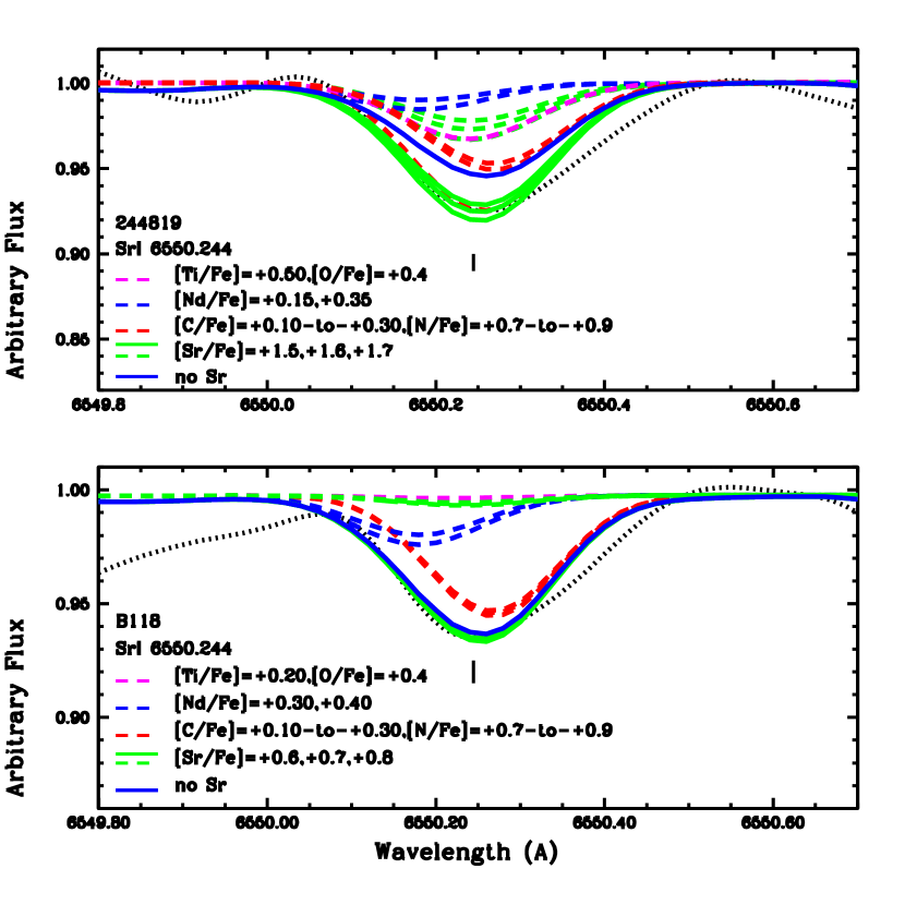
Figure 13: Sr I 6550.244 Å line in stars 244819 and B118, showing the contribution of blends to the line. Observed spectra (black dotted lines) are compared to synthetic spectra for lines as indicated in the panels. Dashed lines correspond to the contribution of a particular element only. Full lines correspond to all lines included. The values [Sr/Fe]=+1.6$\pm$0.1 for 244819 and [Sr/Fe]=+0.7$\pm$0.1 for B118 are indicated by full green lines. These results are not considered reliable, however, due to blends.

Table 8: Abundances in the six UVES sample stars.

species	$\lambda$ (Å)	--$\chi_{ex}$ (eV)	log gf	234816	244523	244819	256289	B118	402370
NaI	5682.633	2.10	$-$0.71	+0.50	+0.00	+0.30	$-$0.40	+0.30	$-$0.30
NaI	5688.194	2.10	$-$1.40	+0.50	$-$0.30	+0.30	$-$0.30	+0.30	$-$0.30
NaI	5688.205	2.10	$-$0.45	+0.50	$-$0.30	+0.30	$-$0.30	+0.30	$-$0.30
NaI	6154.230	2.10	$-$1.56	+0.50	+0.15	+0.50	$-$0.30	+0.30	+0.00:
NaI	6160.753	2.10	$-$1.26	+0.50	+0.25	+0.30	$-$0.30	+0.30	$-$0.30
AlI	6696.185	4.02	$-$1.58	+0.50	+0.30	+0.40	$-$0.30	+0.60	$-$0.30
AlI	6696.788	4.02	$-$1.42	+0.50	—	+0.40	—	—	$-$0.30
AlI	6696.788	4.02	$-$2.72	+0.50	—	+0.40	—	—	$-$0.30
AlI	6698.673	3.14	$-$1.65	+0.50	+0.30	+0.40	$-$0.10	+0.60	$-$0.30
MgI	5528.405	4.34	$-$0.50	+0.70	+0.00	+0.30	+0.30	+0.60	+0.30
MgI	6318.720	5.11	$-$2.10	+0.70	+0.45	+0.30	+0.30	+0.30	+0.30
MgI	6319.242	5.11	$-$2.36	+0.70	+0.30	+0.30	+0.30	+0.30	—
MgI	6319.490	5.11	$-$2.80	+0.70	+0.30	+0.30	+0.30	+0.30	+0.30
MgI	6765.450	5.75	$-$1.94	+0.50	—	—	—	—	+0.25
SiI	5665.555	4.92	$-$2.04	+0.50	—	—	+0.20	+0.20	+0.20
SiI	5666.690	5.62	$-$1.74	+0.50	—	—	—	+0.30	+0.30
SiI	5690.425	4.93	$-$1.87	+0.50	—	—	+0.25	+0.30	+0.20
SiI	5948.545	5.08	$-$1.30	+0.50	+0.30	+0.30	+0.20	+0.30	+0.10
SiI	6142.494	5.62	$-$1.50	+0.50	+0.50	+0.30	+0.30	+0.30	+0.30
SiI	6145.020	5.61	$-$1.45	+0.50	+0.35	+0.30	+0.25	+0.40	+0.30
SiI	6155.142	5.62	$-$0.85	+0.50	+0.35	+0.30	+0.00	+0.30	+0.15
SiI	6237.328	5.61	$-$1.01	+0.50	+0.40	—	+0.15	+0.30	+0.05
SiI	6243.823	5.61	$-$1.30	+0.50	+0.40	+0.20	+0.15	+0.25	+0.30
SiI	6414.987	5.87	$-$1.13	+0.50	+0.45	—	+0.25	+0.30	+0.30
SiI	6721.844	5.86	$-$1.17	+0.50	+0.45	—	+0.15	+0.55	+0.30
CaI	5601.277	2.53	$-$0.52	+0.50	$-$0.30	$-$0.30	$-$0.15	+0.00	+0.12
CaI	5867.562	2.93	$-$1.55	+0.50	+0.20	+0.15	+0.10	$-$0.05	$-$0.10
CaI	6102.723	1.88	$-$0.79	+0.30	$-$0.30	+0.00	+0.30	+0.00	+0.00
CaI	6122.217	1.89	$-$0.20	+0.30	$-$0.30	+0.00	+0.00	+0.00	+0.00
CaI	6156.030	2.52	$-$2.39	+0.40	+0.30	—	+0.05	+0.00	+0.25
CaI	6161.295	2.51	$-$1.02	+0.50	+0.30	+0.30	+0.30	+0.30	+0.30
CaI	6162.167	1.89	$-$0.09	+0.40	$-$0.30	+0.00	+0.40	+0.15	+0.30
CaI	6166.440	2.52	$-$0.90	+0.50	+0.15	+0.15	+0.00	+0.10	+0.00
CaI	6169.044	2.52	$-$0.54	+0.50	+0.00	+0.30	+0.30	+0.25	+0.00
CaI	6169.564	2.52	$-$0.27	+0.50	$-$0.20	+0.15	+0.30	+0.00	+0.00
CaI	6439.080	2.52	+0.3	+0.50	$-$0.30	+0.00	+0.40	$-$0.20	+0.30
CaI	6455.605	2.52	$-$1.35	+0.60	+0.30	—	+0.30	+0.40	+0.15
CaI	6464.679	2.52	$-$2.10	+0.00	—	—	+0.00	—	—
CaI	6493.788	2.52	-2.44	+0.30	+0.00	+0.30	+0.30	$-$0.20	+0.10
CaI	6499.654	2.52	$-$0.85	+0.50	+0.10	+0.30	+0.25	+0.00	+0.10
CaI	6572.779	0.00	$-$4.32	—	+0.30	+0.30	+0.00	+0.30	+0.00
CaI	6717.687	2.71	$-$0.61	—	+0.30	+0.30	…	+0.50	+0.50
TiI	5689.459	2.29	$-$0.44	+0.50	+0.00	+0.30	—	+0.30	+0.00
TiI	5866.449	1.07	$-$0.84	+0.50	+0.15	+0.30	+0.00	+0.10	+0.00
TiI	5922.108	1.05	$-$1.46	+0.50	+0.20	+0.15	+0.00	+0.30	+0.00
TiI	5941.750	1.05	$-$1.5	+0.60	+0.30	+0.30	+0.00	+0.30	+0.00
TiI	5965.825	1.88	$-$0.42	+0.50	+0.30	+0.10	+0.00	+0.30	+0.10
TiI	5978.539	1.87	$-$0.53	+0.50	+0.35	+0.25	+0.00	+0.30	+0.00
TiI	6064.623	1.05	$-$1.94	+0.60	+0.30	+0.10	—	—	+0.00
TiI	6091.169	2.27	$-$0.42	+0.60	+0.30	+0.10	+0.00	+0.20	+0.00
TiI	6126.214	1.07	$-$1.43	+0.55	+0.30	+0.15	+0.10	+0.30	+0.00
TiI	6258.110	1.44	$-$0.36	+0.30	+0.05	$-$0.30	$-$0.15	$-$0.30	+0.15
TiI	6261.106	1.43	$-$0.48	+0.60	+0.20	+0.05	$-$0.10	+0.00	+0.00
TiI	6266.010	1.75	$-$2.98	—	—	—	—	—	—
TiI	6303.767	1.44	$-$1.57	+0.50	+0.30	+0.25	+0.00	+0.30	+0.00
TiI	6312.240	1.46	$-$1.60	+0.60	+0.30	+0.30	+0.10	+0.30	+0.00
TiI	6336.113	1.44	$-$1.74	+0.55	—	+0.30	—	+0.20	$-$0.15
TiI	6508.150	1.43	$-$2.05	—	—	—	—	—	—
TiI	6554.238	1.44	$-$1.22	+0.35	+0.30	+0.15	—	+0.40	$-$0.30
TiI	6556.077	1.46	$-$1.07	+0.50	+0.30	+0.30	+0.00	+0.30	+0.00
TiI	6599.113	0.90	$-$2.09	+0.60	+0.40	+0.30	+0.00	+0.35	+0.00
TiI	6743.127	0.90	$-$1.73	+0.50	+0.30	+0.30	+0.00	+0.30	$-$0.10
TiII	5336.771	1.58	$-$1.70	+0.50	+0.10	+0.30	+0.00	—	+0.30
TiII	5381.0212	1.57	$-$2.08	+0.50	+0.10	+0.30	+0.00	$-$0.30	+0.00
TiII	5418.751	1.58	$-$2.13	+0.50	+0.30	+0.50	+0.20	$-$0.20	+0.10
TiII	6491.580	2.06	$-$2.10	+0.35	+0.30	+0.30	+0.30	+0.40	+0.15
TiII	6559.576	2.05	$-$2.35	+0.35	+0.30	+0.30	+0.30	+0.30	+0.30
TiII	6606.970	2.06	$-$2.85	+0.50	+0.30	—	+0.20	+0.25	+0.15
Y I	6435.004	0.07	$-$0.82	+0.50	+0.80	+0.80	$-$0.15	+0.30	+0.30
Y II	6795.414	1.74	$-$1.19	+0.30	+0.50	+1.00:	+0.30	+0.40	+0.00
Zr I	6127.475	0.15	$-$1.06	+0.50	—	—	+0.15	+0.50:	—
Zr I	6134.585	0.00	$-$1.426	+0.65	—	—	+0.10	+0.50:	—
Zr I	6140.535	0.52	$-$1.6	—	—	—	+0.10	—	—
Zr I	6143.252	0.07	$-$1.1	+0.65	—	—	+0.10	+0.50	—
Ba II	5853.675	0.60	$-$1.1	+0.50	+0.65	+0.30	+0.30	+0.15	+0.60
Ba II	6141.713	0.70	$-$0.08	+0.50	+0.60	+0.30	+0.30	+0.00	+0.60
Ba II	6496.897	0.60	$-$0.32	+0.60	+0.65	+0.50	+0.50	+0.30	+0.80
La II	6262.287	0.40	$-$1.60	+0.40	+1.00	+0.40	+0.00	+0.60	+0.00
La II	6320.376	0.17	$-$1.56	+0.30	+0.80	+0.30	+0.00	+0.50	+0.00
La II	6390.477	0.32	$-$1.41	+0.40	+0.90	+0.40	+0.00	+0.60	+0.10
Nd II	6549.525	0.06	$-$2.01	+0.30	+0.60	—	+0.00	+0.30	+0.00
Nd II	6740.078	0.06	$-$1.53	+0.00	+0.80	+0.30	+0.00	+0.30	+0.00
Nd II	6790.372	0.18	$-$1.77	+0.30	+0.80	+0.00	+0.00	+0.30	-0.30
Eu II	6173.029	1.32	$-$0.86	+0.80:	—	—	—	—	—
Eu II	6437.640	1.32	$-$0.32	+0.80	+0.80	+0.50	+0.40	+0.50	+0.50:
Eu II	6645.064	1.38	+0.12	+0.80	+0.50	+0.50	+0.45	+0.60	+0.50

Table 9: Mean abundances of C, N, odd-Z elements Na, Al, $\alpha$-elements O, Mg, Si, Ca, Ti, and heavy elements Y, Zr, Ba, La, and Eu. The four stars analysed in Barbuy et al. (2014) are also included. For the mean values, only the eight member stars were considered.

star

[C/Fe]

[N/Fe]

[Na/Fe]

[Al/Fe]

[O/Fe]

[Mg/Fe]

[Si/Fe]

[Ca/Fe]

[TiI/Fe]

[TiII/Fe]

[Y/Fe]

[Zr/Fe]

[Ba/Fe]

[La/Fe]

[Nd/Fe]

[Eu/Fe]

The two non-member stars

234816

$<$0.2

+0.80

+0.50

+0.50

+0.60

+0.66

+0.50

+0.42

+0.52

+0.45

+0.40

+0.60

+0.53

+0.36

+0.20

+0.80

244523

$<$0.2

$<$0.8

-0.04

+0.30

+0.40

+0.26

+0.40

+0.02

+0.26

+0.18

+0.65

—

+0.63

+0.90

+0.70

+0.65

Four stars from the present work

244819

$<$0.2

$<$1.2

+0.34

+0.40

+0.40

+0.30

+0.28

+0.14

+0.19

+0.34

+0.90

—

+0.36

+0.36

+0.15

+0.50

256289

$<$0.2

$<$0.3

$-$0.32

$-$0.20

+0.40

+0.30

+0.19

+0.18

+0.00

+0.17

+0.08

+0.11

+0.36

+0.00

+0.00

+0.43

B118

$\mathrel{\hbox{\raise 2.15277pt\hbox{$<$}\hbox to0.0pt{\hss\lower 2.15277pt\hbox{$\sim$}}}}$0.2

$<$0.8

+0.30

+0.60

—

+0.40

+0.32

+0.10

+0.23

+0.09

+0.35

+0.50

+0.15

+0.57

+0.30

+0.55

402370

$<$0.0

$<$0.3

$-$0.24

$-$0.30

+0.40

+0.29

+0.23

+0.13

$-$0.02

+0.16

+0.15

—

+0.66

+0.03

-0.10

+0.50

Four stars from Barbuy et al. (2014)

B-107

+0.00

—

+0.03

+0.28

+0.50

+0.33

+0.17

+0.16

+0.03

+0.17

+0.32

+0.20

+0.45

+0.20

—

+0.40

B-122

$-$0.20

+0.70

+0.09

+0.18

+0.20

+0.10

+0.06

+0.00

+0.03

+0.15

+0.20

+0.10

+0.05

+0.35

—

+0.30

B-128

+0.10

+0.60

+0.01

+0.08

+0.23

+0.23

+0.14

+0.20

+0.05

+0.17

+0.43

+0.40

+0.55

+0.35

—

+0.30

B-130

+0.00

+0.70

+0.05

+0.26

+0.50

+0.27

+0.13

+0.15

+0.03

+0.18

+0.23

+0.00

+0.22

+0.00

—

+0.20

Mean

$\sim$+0.14

+0.66

+0.09

+0.24

+0.38

+0.28

+0.19

+0.13

+0.07

+0.18

+0.33

+0.23

+0.35

+0.23

+0.09

+0.40

Table 10: Heavy element abundance ratios.

star	[Ba/La]	[Ba/Eu]	[La/Eu]	[Y/Ba]	[Y/La]
234816	+0.17	$-$0.27	$-$0.44	$-$0.13	+0.04
244523	$-$0.27	$-$0.02	+0.25	+0.02	$-$0.25
244819	+0.00	$-$0.14	$-$0.14	+0.54	+0.54
256289	+0.36	$-$0.07	$-$0.43	$-$0.28	+0.08
B118	$-$0.42	$-$0.40	+0.02	+0.20	$-$0.22
402370	+0.63	+0.16	$-$0.47	-0.51	+0.12
B-107	+0.25	+0.05	$-$0.20	$-$0.13	+0.12
B-122	$-$0.30	$-$0.25	+0.05	+0.15	$-$0.15
B-128	+0.20	+0.25	+0.05	$-$0.12	+0.08
B-130	+0.22	+0.02	$-$0.20	+0.01	+0.23

5.4 Errors

Uncertainties in spectroscopic parameters are given in Table 12 for star NGC 6522: 402370. For each stellar parameter, we adopted the usual uncertainties as for similar samples (Barbuy et al. 2014, 2016, 2018b): $\pm$100 K in effective temperature, $\pm$0.2 on gravity, and $\pm$0.2 km s^-1 on the microturbulence velocity. Errors were computed by employing models with these modified parameters, with changes of $\Delta$T${\rm eff}$=+100 K, $\Delta$log g =+0.2, $\Delta$v_t = 0.2 km s^-1, and recomputing lines of different elements. The error given is the abundance difference needed to reach the adopted abundances. Uncertainties due to non-LTE effects are negligible for these stellar parameters as discussed in Ernandes et al. (2018). The same error analysis and estimations can be applied to other stars in our sample. A more careful discussion is required for Ba. The heavy element abundances for star B118 reported in Table 11 show that the abundance ratios are confirmed from one work to another, except for Ba. This is due to the use of strong lines that fall in the saturated part of the curve of growth, where the abundance is a function of the square root of the number of atoms; the bottom of the lines reaches a maximum, and the increase of abundance causes an increase in the line wings. Therefore, abundance derivations from strong lines are in general avoided, since they are too sensitive to stellar parameters and spectral resolution. The La lines are, on the other hand, faint and they are at least not affected by the same problem.

Finally, it is important to note that the main uncertainties in stellar parameters are due to uncertainties in the effective temperature, as can be seen in Table 5. The second most important source of error are the EWs, given the limited S/N of the spectra, which can be estimated using the formula from Cayrel (1988): $\sigma_{EW}$ = 1.5 $\sqrt{FWHM.\delta_{x}}/(S/N)$, where $\delta_{x}$ is the pixel size. The difference in the mean metallicities between the present work and Barbuy et al. (2014) are probably due to a difference in the measurements of EWs, and in particular in the placement of continua.

Table 11: Heavy element results for star B118 from Barbuy et al. (2009, B09), Chiappini et al. (2011, C11), Ness et al. (2014, N14) and present work.

work	Teff	log g	[Fe/H]	vrmt	[Y/Fe]	[Zr/Fe]	[Sr/Fe]	[Ba/Fe]	[La/Fe]	[Eu/Fe]
B09	4700	2.6	$-$0.84	1.30	—	—	—	+1.00	+0.50	+0.50
C11	same	same	same	same	+0.50	—	+1.50	same	same	same
N14	5000	2.25	$-$1.04	2.45	+0.30	—	—	+0.30	+0.55	+0.40
this	4820	2.20	$-$1.17	2.10	+0.25	+0.50	+0.70	+0.15	+0.57	+0.55

Comparison between results from UVES and GIRAFFE spectra: For the sample stars, we have the UVES spectra ranging from 4800-5800 Å, with a gap at 5777-5824 Å, and the GIRAFFE spectra in the setups H11 (5597-5840) and H12 (5821-6146) only. Therefore, since most lines used for the stellar parameter analysis are in the UVES red arm, and most lines for deriving abundances are also in the UVES red arm, we cannot compare the stellar parameter derivation. Moreover, we only compare the main lines in common between the two sets of spectra, which are located at $\lambda$$<$6142 Å.

By comparing the abundances for a list of lines in common between UVES and GIRAFFE, we give another indicator of uncertainty. In Table 13, we compare the abundances derived from UVES spectra to those derived from GIRAFFE spectra. The results show an excellent agreement. In order to be clear, the stellar parameters are much better derived from UVES spectra, in particular because of the measurement of the Fe II lines; whereas, given a set of stellar parameters, the abundances from the same lines at the different resolutions are both reliable.

Table 12: Abundance uncertainties for star N6522:402370, for uncertainties of $\Delta$T_eff = 100 K, $\Delta$log g = 0.2, $\Delta$v_t = 0.2 km s^-1 and corresponding total error. The errors are to be added to reach the reported abundances.

Element	$\Delta$T	$\Delta$log $g$	-$\Delta$vt	-($\sum$x2)1/2
	100 K	0.2 dex	0.2 kms-1
(1)	(2)	(3)	(4)	(5)
[FeI/H]	$-$0.10	+0.01	+0.05	+0.11
[FeII/H]	+0.10	$-$0.07	+0.04	+0.13
[C/Fe]	+0.02	+0.02	+0.00	+0.03
[O/Fe]	+0.00	+0.05	+0.00	+0.05
[NaI/Fe]	+0.05	+0.00	+0.00	+0.05
[AlI/Fe]	+0.06	+0.00	+0.00	+0.06
[MgI/Fe]	+0.00	+0.01	+0.00	+0.01
[SiI/Fe]	+0.03	+0.00	+0.00	+0.03
[CaI/Fe]	+0.08	+0.00	+0.01	+0.08
[TiI/Fe]	+0.12	+0.01	+0.00	+0.12
[TiII/Fe]	$-$0.05	+0.07	+0.00	+0.09
[YI/Fe]	+0.15	+0.04	+0.00	+0.10
[YII/Fe]	+0.20	+0.15	+0.00	+0.25
[ZrI/Fe]	+0.20	$-$0.01	+0.00	+0.20
[BaII/Fe]	+0.10	+0.15	$-$0.15	+0.23
[LaII/Fe]	+0.05	+0.15	+0.00	+0.16
[LaII/Fe]	+0.12	+0.05	+0.00	+0.13
[EuII/Fe]	$-$0.05	+0.05	+0.00	+0.07

Table 13: Comparison of abundances from UVES and GIRAFFE.

species	$\lambda$ (Å)	234816	234816	244523	244523	244819	244819	256289	256289	B118	B118	402370	402370
		UVES	GIRAFFE	UVES	GIRAFFE	UVES	GIRAFFE	UVES	GIRAFFE	UVES	GIRAFFE	UVES	GIRAFFE
Na I	5682.633	+0.50	+0.50	+0.00	+0.00	+0.30	+0.30	-0.40	$-$0.30	+0.30	+0.40	$-$0.30	+0.00
Na I	5688.194	+0.50	+0.50	$-$0.30	+0.00	+0.30	+0.30	$-$0.30	$-$0.30	+0.30	+0.50	$-$0.30	+0.00
Na I	5688.205	+0.50	+0.50	$-$0.30	+0.00	+0.30	+0.30	$-$0.30	$-$0.30	+0.30	+0.50	$-$0.30	+0.00
Si I	5665.555	+0.50	+0.50	—	+0.35	—	+0.35	+0.20	+0.00	+0.20	+0.35	+0.20	+0.00
Si I	5666.690	+0.50	—	—	—	—	—	—	+0.00	+0.30	+0.00	+0.30	+0.30
Si I	5690.425	+0.50	+0.50	—	+0.50	—	+0.35	+0.25	+0.20	+0.30	+0.30	+0.20	—
Si I	5948.545	+0.50	+0.00	+0.30	+0.15	+0.30	+0.30	+0.20	+0.00	+0.30	+0.15	+0.10	+0.00
Si I	6142.494	+0.50	+0.50	+0.50	—	+0.30	—	+0.30	—	+0.30	+0.15	+0.30	+0.30
Ca I	5601.277	+0.50	+0.50	$-$0.30	+0.10	$-$0.30	+0.30	$-$0.15	+0.15	+0.00	+0.30	+0.12	+0.00
Ca I	5867.562	+0.50	+0.50	+0.20	+0.30	+0.15	+0.30	+0.10	+0.10	$-$0.05	+0.30	$-$0.10	+0.00
Ca I	6102.723	+0.30	+0.30	$-$0.30	+0.00	+0.00	+030	+0.30	+0.30	+0.00	+0.15	+0.00	+0.15
Ca I	6122.217	+0.30	+0.30	$-$0.30	+0.00	+0.00	+0.30	+0.00	+0.15	+0.00	+0.00	+0.00	+0.00
Ti I	5689.459	+0.50	+0.50	+0.00	+0.30	+0.30	+0.30	—	—	+0.30	+0.30	+0.00	—
Ti I	5866.449	+0.50	+0.50	+0.15	+0.20	+0.30	+0.30	+0.00	+0.00	+0.10	+0.15	+0.00	+0.00
Ti I	5922.108	+0.50	+0.50	+0.20	+0.45	+0.15	+0.30	+0.00	+0.00	+0.30	+0.30	+0.00	+0.00
Ti I	5941.750	+0.60	+0.50	+0.30	+0.50	+0.30	+0.30	+0.00	+0.20	+0.30	—	+0.00	+0.00
Ti I	5965.825	+0.50	+0.50	+0.30	+0.30	+0.10	+0.30	+0.00	+0.00	+0.30	+0.30	+0.10	+0.00
Ti I	5978.539	+0.50	+0.50	+0.35	+0.30	+0.25	+0.30	+0.00	+0.00	+0.30	+0.30	+0.00	+0.00
Ti I	6064.623	+0.60	+0.50	+0.30	+0.30	+0.10	+0.30	—	+0.00	—	+0.15	+0.00	+0.00
Ti I	6091.169	+0.60	+0.50	+0.30	+0.30	+0.10	+0.30	+0.00	—	+0.20	+0.30	+0.00	+0.00
Ti I	6126.214	+0.55	+0.50	+0.30	+0.30	+0.15	+0.30	+0.10	+0.00	+0.30	+0.30	+0.00	+0.00
Zr I	6127.475	+0.50	+0.50	—	+0.30	—	—	+0.15	+0.30	+0.50:	+0.50:	—	—
Zr I	6134.585	+0.65	+0.50	—	+0.50	—	—	+0.10	—	+0.50:	—	—	—
Zr I	6140.535	—	—	—	—	—	—	+0.10	—	—	—	—	—
Zr I	6143.252	+0.65	+0.50	—	—	—	—	+0.10	—	+0.50	+0.30	—	—
Ba II	5853.675	+0.50	+0.50	+0.50	+0.60	+0.30	+0.30	+0.30	+0.30	+0.00	+0.20	+0.60	+0.30
Ba II	6141.713	+0.50	+0.40	+0.40	—	+0.30	—	+0.30	—	$-$0.30	$-$0.30	+0.60	+0.15

6 Discussion

The inspection on abundances of heavy elements in NGC 6522 was triggered by the variation in Ba abundances reported in Barbuy et al. (2009). In C11, we tentatively tried to connect these abundances with the s-process nucleosynthesis calculations in spinstars first presented by Pignatari et al. (2008) and computed by Frischknecht et al. (2012). We did so for a spinstar of 40 M_⊙, a metallicity of [Fe/H] = $-$3.8, and a rotational velocity of V_rot = 500 km.s^-1. The lower resolution data (R$\sim$22,000) from GIRAFFE spectra were compatible with the s-process yields of spinstars boosted by up to four orders of magnitude with respect to a non-rotating star of the same mass and metallicity (see their Fig. 2).

A next step was presented in Barbuy et al. (2014), where the analysis of higher resolution data from UVES (R$\sim$45,000), was studied in terms of an extended grid of spinstar models from Frischknecht et al. (2016). This paper reported enhancement of the heavy elements Sr, Y, La, and Ba measurable in stellar spectra. The new results were shown to be compatible with expectations from massive spinstars, but allowing for other mechanisms to be invoked.

In a third step using the observations of 2012, besides the four stars observed with UVES and reported in Barbuy et al. (2014), we also identified possible new cluster member stars from the GIRAFFE spectra. In 2016, we obtained new UVES observations of six such newly identified member stars, which we analyse here.

6.1 Analysis of the present results

We derived a mean metallicity of [Fe/H]=$-$1.16$\pm$0.05, somewhat lower than the B09, B14, and Fernández-Trincado et al. (2019) values of [Fe/H]= -1.0, -0.95 and -1.04, respectively, and closer to the value of [Fe/H] = -1.15 from Ness et al. (2014). By gathering the metallicities of the present four member stars and the other four stars from Barbuy et al. (2014), we obtain [Fe/H]=$-$1.05$\pm$0.20.

The mean abundances for the six sample stars, as well as the four stars studied in Barbuy et al. (2014), are reported in Table 9. In the mean we see a normal expected enhancement of the bona fide alpha elements O and Mg, and a mild enhancement of Si and Ca (and Ti, noting that Ti behaves as an alpha, but it is an iron-peak element). There has been evidence that the alpha elements O and Mg formed during the hydrostatic phases of massive stars nucleosynthesis are more enhanced than the other alpha elements, Si, Ca, and Ti, which are formed predominantly during explosive nucleosynthesis (Woosley & Weaver 1995, McWilliam 2016).

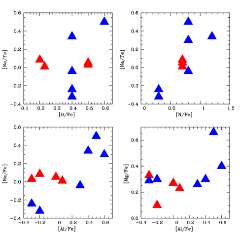
Figure 14: [Na/Fe] versus [O/Fe] anti-correlation in NGC 6522 stars compared with stars in NGC 6121; and [Na/Fe] versus [N/Fe], [Al/Fe] and [Mg/Fe] versus [Al/Fe] correlations. Symbols: blue-filled triangles represent the present results for NGC 6522; red-filled triangles denote results for NGC 6522 from Barbuy et al. (2014).

The enhancements of N, Na, and Al vary from star to star, indicating that some stars are probably second generation ones. We note that the enhancement in N is also due to a large scatter in its early enrichment history (e.g. Cescutti & Chiappini 2010) as well as stellar evolution effects. In Fig. 14, we do not find a clear anti-correlation between the [O/Fe] and [Na/Fe] ratios in our stellar sample, such as, for instance, in NGC 6121, which is a well-populated cluster in this diagram (Carretta et al. 2009). In Fig. 14,we also show the correlated abundance signatures of [Al/Fe] versus [Na/Fe], [N/Fe] versus [Na/Fe], and [Mg/Fe] versus [Al/Fe]. These diagrams confirm the presence of at least two stellar populations in NGC 6522, as found by Kerber et al. (2018) from photometry.

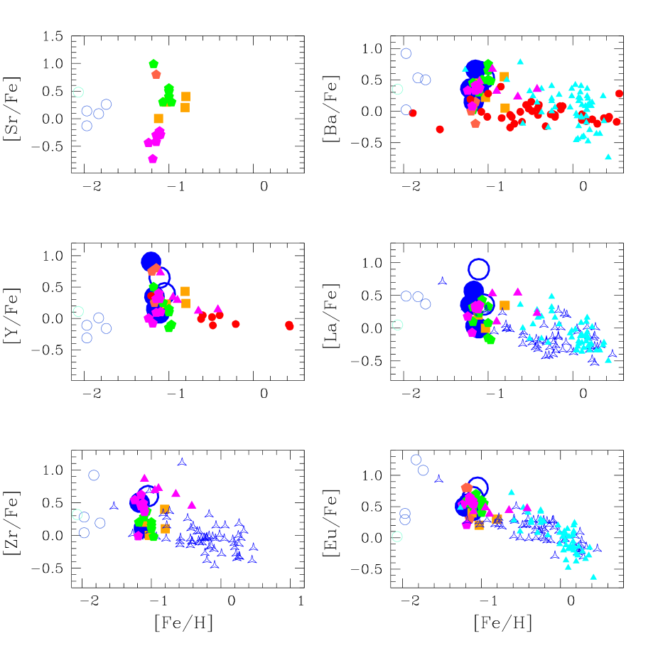
Figure 15: [Sr,Y,Zr,Ba,La,Eu/Fe] versus [Fe/H] in bulge stars. Symbols: Large, blue-filled circles mark present results of NGC 6522 member stars; large, blue open circles represent the present results of non-member stars. Field stars: Blue open triangles represent red giants by Johnson et al. (2012); magenta-filled triangles represent red giants by Siqueira-Mello et al. (2016); cyan-filled triangles denote red giants by van der Swaelmen et al. (2016); red-filled circles show dwarfs by Bensby et al. (2017); light blue open circles mark metal-poor giants by Howes et al. (2016); acquamarine open circles show metal-poor giants by Lamb et al. (2017). Globular cluster stars: Orange-filled squares show NGC 6522 (Barbuy et al. 2014); green-filled pentagons mark HP 1 (Barbuy et al. 2016); tomato-filled pentagons represent NGC 6558 (Barbuy et al. 2018); magenta-filled pentagons show M62 (Yong et al. 2014).

For the heavy elements, we present the plot of abundances including the new results. In Fig. 15, we compare the present results on heavy element abundances of Sr, Y, Zr, La, Ba, and Eu relative to Fe, together with those from Barbuy et al. (2014) for another four stars in NGC 6522. Literature abundances from field bulge red giants are from Johnson et al. (2012), for Zr, La, and Eu in Plaut’s field, Siqueira-Mello et al. (2016), van der Swaelmen et al. (2016), and metal-poor giants from Howes et al. (2016) and Lamb et al. (2017). Also included are the abundances Bensby et al. (2017 and references therein) for 39 microlensed bulge dwarfs and subgiants that are older than 9.5 Gyr, selected among their 90 stars. Finally, abundances in the bulge globular cluster HP 1 (Barbuy et al. 2016), NGC 6558 (Barbuy et al. 2018b), and M62 (Yong et al. 2014) are also shown.

From Fig. 15, the most striking feature is the abundance variation of Sr, Y, Zr, and to lesser extent Ba and La at the metallicity of [Fe/H] $\sim$ $-$1.0, where the bulge globular clusters are found. For Sr, we report literature data only, given the unreliability of Sr derivation in the present sample due to blends with CN and C₂ lines. We note that the spread is clearly larger in halo metal-poor stars with [Fe/H]$\mathrel{\hbox{\raise 2.15277pt\hbox{$<$}\hbox to0.0pt{\hss\lower 2.15277pt\hbox{$\sim$}}}}$-2.5 (Cescutti et al. (2013), Hansen et al. (2014). For Eu, the behaviour of [Eu/Fe] versus [Fe/H] is more well-defined, indicating a spread at low metallicities and a declining abundance ratio with increasing metallicities.

From Table 9 and Fig. 15, we find that a) Y tends to be enhanced, showing strong star-to-star variations; b) Ba tends to be enhanced, showing star-to-star variations. and c) Eu is enhanced similarly to the alpha elements O and Mg.

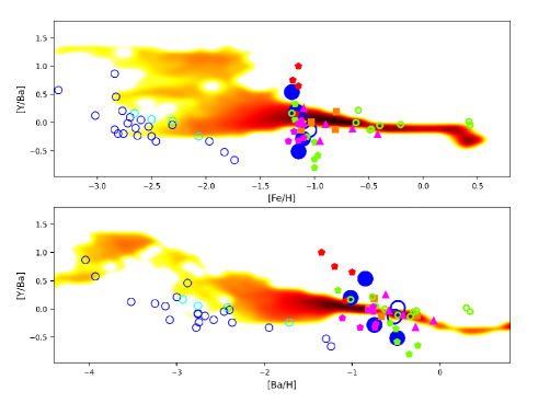
Figure 16: [Y/Ba] vs. [Fe/H] (upper panel) and [Y/Ba] versus [Ba/H] (lower panel). Symbols: Large blue-filled circles show present results on NGC 6522 member stars; large blue open circles show present results on non-member stars. Field stars: Magenta-filled triangles denote red giants by Siqueira-Mello et al. (2016); green open circles mark dwarfs by Bensby et al. (2017); light blue open circles show metal-poor giants by Howes et al. (2016); acquamarine open circles represent metal-poor giants by Lamb et al. (2017). Globular cluster stars: Orange-filled squares show NGC 6522 (Barbuy et al. 2014); green-filled pentagons represent HP 1 (Barbuy et al. 2016); tomato-filled pentagons show NGC 6558 (Barbuy et al. 2018); magenta-filled pentagons represent M62 (Yong et al. 2014). The underlying coloured model corresponds to calculations for nucleosynthesis taking place in spinstars and in MRD supernovae (Cescutti et al. 2018 and references therein).

As mentioned, Y and Ba variations are compatible with a large number of nucleosynthesis processes, with the member stars 244819 and B118 showing [Y/Ba] excesses of +0.54 and +0.35, respectively. The observation of more heavy elements would be necessary to differentiate between the potential astrophysical sources. The variation in [Y/Ba] data compared with a chemical evolution model for the Galactic bulge is shown in Figure 16.

We note that in C11 there was no model, but instead a calculation for only one mass and that was showing the impact of rotation already. The argument was that even if that calculation was done for a very metal-poor metallicity, because in the bulge the metallicity grows quickly, we would see its effect in the very old bulge stars at [Fe/H] $-$1.0 as well.

In Fig. 16, we present the result of stochastic models, as presented in Cescutti et al. (2018). This can be summarised as follows. The nucleosynthesis adopted for the s process from rotating massive stars comes from Frischknecht et al. (2016). In this set of yields, the s process for massive stars is computed for a rotation velocity of v_ini/v_crit = 0.4 and is composed of a grid of four stellar masses (15, 20, 25, and 40 M_⊙) and three metallicities (solar metallicity, 10^-3, 10^-5) (Cescutti & Chiappini 2014, Cescutti et al. 2013). The model considers the enrichment produced by r-process events as originated from magneto-rotationally driven supernovae (MRD SNe; see Winteler et al 2012, Nishimura et al. 2017); MRD SNe are assumed to be 10% of all the SNe II. The model also takes into account the s-process production from 1.5 to 3 M_⊙ stars and SNIa enrichment, as in Cescutti et al. (2006). In summary, this model considers the fact that the enrichment in heavy elements takes place both in spinstars and in MRD supernovae.

A spread in abundances of these elements is observed in metal-poor halo stars (e.g. François et al. 2003; Cescutti & Chiappini 2014; Rizzutti et al. 2021) and is expected from spinstar models (Frischknecht et al. 2012, 2016; Choplin et al. 2018, Limongi $\&$ Chieffi 2018) and from the contribution of neutrino-driven winds in CCSNe (e.g. Roberts et al. 2010). The observed heavy element abundance ratios tend to show a higher spread of abundance ratios at the metallicity of NGC 6522 relative to the models.

However, the models presented in Fig. 16 were optimised for old field stars of the Galactic bulge, adopting the same nucleosynthesis that worked well for the Galactic halo (Cescutti et al. 2013). Although this model is not specifically made for a globular cluster, it is still useful. For instance, it shows the extension of the dispersion that the enrichment due to rotating massive stars can produce on these abundance ratios. The goal is to show that the predicted scatter is indeed compatible with the dispersion observed in NGC 6522. However, this scatter in field stars seems to appear at lower metallicities (see Barbuy et al. 2018 where our model is compared with field bulge stars). It is then plausible that other physical mechanisms are at play in the cluster evolution (involving dynamical effects, and mass loss through winds). The model for the field bulge stars would just give an idea of the mean cluster abundances but not its scatter. A detailed description of the models presented in Fig. 16, with a focus on the expected differences in the abundance ratio scatter in the bulge and halo, will be presented in Cescutti et al. (2021, in preparation).

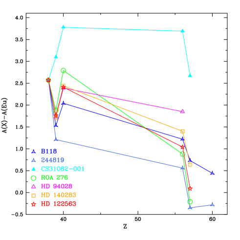
Figure 17: A(X)-A(Eu) versus atomic number Z for stars B118 and 244819 compared with stars CS 31082-001, ROA 276, HD 94028, HD 140283, and HD 122563. All abundances are normalised to the Sr abundance of B118. Symbols are identified in the figure panel.

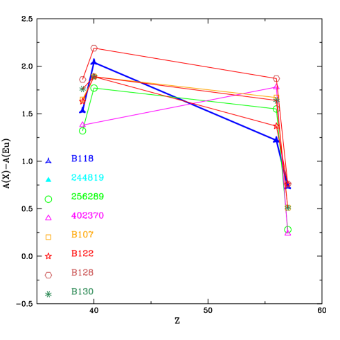
Figure 18: A(X)-A(Eu) versus atomic number Z for star B118 compared with the other seven sample stars. The abundances are not normalised. Symbols are identified in the figure panel.

In order to better interpret the heavy-element abundances of star B118, in Fig. 17 we show the abundance pattern of stars 244819 and B118 in terms of A(X)-A(Eu) (where A(X)=log(N_X/N_H+12), in a diagram idealised by Honda et al. (2007) and Roederer et al. (2010, their Fig. 11). In this figure, A(X)-A(Eu) versus Z of 244819 and B118 are compared with data from the typical r-element star CS 31082-001 (Hill et al. 2002), and the typical LEPP star HD 122563 (Honda et al. 2007, Montes et al. 2007), the identified spinstar-enriched star ROA 276 in $\omega$ Centauri (Yong et al. 2017), and the reference dwarf stars HD 94028 and HD 140283 (Peterson et al. 2020; Siqueira-Mello et al. 2015). First of all, Figure 17 indicates that 244819 and B118 are weakly enriched in r elements. Figure 18 shows A(X)-A(Eu) versus Z for the four member stars from this paper plus the four stars from Barbuy et al. (2014) for Y, Zr, Ba, and La. It shows that the sample stars essentially follow the same pattern, whereas 244819 and B118 show a larger abundance difference between first peak and second peak elements.

Spite et al. (2018) suggested that the heavy element enrichment should take place first due to a pure r process, followed by an enrichment of first-peak elements only, and that this second mechanism would be detectable only in weak-r-process stars. On the other hand, spinstars could be progenitors of magneto-rotational supernovae, but in case the conditions do not allow r-process elements to form in the final explosion, it is also possible that we can only observe the signature of the s-process production in spinstars today.

There are a number of points that it is important to consider in our analysis. First of all, the s-process efficiency in spinstars varies greatly if we consider different theoretical stellar yields. While for instance the s-process production in models by Frischknecht et al. (2016) and Choplin et al. (2018) would stop in the Ba mass region, in models by Limongi $\&$ Chieffi (2018) heavier elements up to lead could be produced. This uncertainty of course affects Galactic chemical evolution (GCE) predictions (e.g. Cescutti et al. 2013, Rizzuti et al. 2019, Prantzos et al. 2020, Rizzuti et al. 2021). Additionally, CCSNe generated from slowly rotating progenitors or spinstars can also eject other nucleosynthesis components made before the SN explosion (similarly to the intermediate neutron capture process or i process - see e.g. Roederer et al. 2016 and Banerjee et al 2018) or by explosion (similarly to the zoo of neutrino-driven wind components - see e.g. Qian $\&$ Wasserburg 2008, Farouqi et al. 2009, Roberts et al. 2010, Arcones $\&$ Montes 2011). As we mentioned earlier, all of these processes may contribute to the production of Sr, Y, and Zr, while at low metallicities the i process can potentially produce elements across the whole mass region below and beyond Fe, including Sr, Y, Zr, and Ba, in different types of stars (e.g. Abate et al. 2016, Roederer et al. 2016, Clarkson et al. 2018, Banerjee et al 2018). For instance, the high [Ba/La] in stars 256289, 402370, B-107, B-128, and B-130 would be compatible with the i process (see e.g. Hampel et al. 2016).

Alternative possibilities of neutron-capture element enrichment are the magneto-rotationally driven explosions of core-collapse supernovae (Winteler et al. 2012), or s process taking place in asymptotic giant branch (AGB) stars and subsequent mass transfer within a binary system (e.g. Cristallo et al. 2015). A study on possible nucleosynthesis processes is given in Hansen et al. (2014).

This makes the observation of more elements per stellar target and at high resolution of different stars in globular clusters such as NGC 6522 crucial. Within this scenario the large star-to-star variations of heavy-element enrichment could be a natural outcome of an intrinsic scatter of s-process efficiencies in spinstars or the varying contribution of different processes active before and during SN explosions in massive stars. On the other hand, when abundances of several heavy elements are available it becomes possible to disentangle the dominant nucleosynthesis component(s) that made the whole observed abundance pattern (see e.g., Roederer et al. 2016, Peterson et al. 2020). Stars in NGC 6522 are carriers of the same signatures of the nucleosynthesis processes active in the early galaxy and observed in halo stars, even if they are more metal-rich as a result of a steeper age-metallicity relation in the Galactic bulge (as suggested in C11).

6.2 The two non-member stars 234816 and 244523

The stars 234816 and 244523 have the correct magnitudes, radial velocities and metallicities to be members of NGC 6522. However, the Gaia proper motions reported in Table 3 rule out their membership.

Could these two stars be former members that are evaporating from the cluster? Madrid et al. (2017) studied evaporation rates as a function of galactocentric distance R_GC and time and predicted a very high evaporation at low R_GC due to the strong tidal field in the central parts of the Galaxy. NGC 6522 is estimated to have a mass of 5.93$\times$10⁴ M_⊙ (Gnedin & Ostriker 1997), which is not high for a globular cluster. It is located at R_GC $\approx$ 1 kpc and has an age above 12.1 - 12.4 Gyr using Dotter et al. (2008) isochrones and even older (with 14.1 - 14.2 Gyr) using BaSTI isochrones (Kerber et al. 2018). It can be seen from Fig. 6 of Madrid et al. (2017) that the evaporation rate in a bulge cluster like NGC 6522 should be extremely high. It is therefore acceptable to suggest that the two stars could be evaporating from the cluster. However, a more detailed orbital calculation would be needed to check this possibility, such as the one carried out by Hanke et al. (2020). In particular, star 234816 has different alpha-element abundances and should not be a member.

7 Conclusions

We derived a mean metallicity of [Fe/H]=$-$1.16$\pm$0.05 from the four sample stars. Combined with the other four stars from Barbuy et al. (2014), the result is a mean metallicity of [Fe/H]=$-$1.05$\pm$0.20.

Among the six stars analysed, two of them are indicated to be non-members from Gaia proper motions; still, they have the correct magnitude, radial velocity, and metallicity to be members. Only a fraction of about 0.5% of stars in the Galactic bulge have metallicities below [Fe/H]$\mathrel{\hbox{\raise 2.15277pt\hbox{$<$}\hbox to0.0pt{\hss\lower 2.15277pt\hbox{$\sim$}}}}$-1.0 (Barbuy et al. 2018a). Therefore, we suggest that these stars could be evaporating from the cluster; but even so, we do not include their abundances in the discussion below. Star 244523 has abundances compatible with the member stars. Star 234816 shows different high alpha-element abundances, and it could be an intruder; hence, it could have been a bulge star with the correct magnitude and metallicity to be considered a member before we had Gaia measurements, but it was eventually revealed as a non-member star.

For the present results on the four confirmed member stars, together with those by Barbuy et al. (2014), the alpha-elements show enhancements of [O/Fe]=+0.38, [Mg/Fe]=$\approx$+0.28, [Si/Fe]$\approx$+0.19, and [Ca/Fe]$\approx$+0.13, [Ti/Fe]$\approx$+0.13. A higher enhancement in O and Mg, and a lower one in Si, Ca, and Fe can be explained by their formation in hydrostatic conditions for the former, and in explosive nucleosynthesis for the latter (e.g. Woosley & Weaver 1995; McWilliam 2016).

The r-process element Eu is enhanced by [Eu/Fe]=+0.40. The $\alpha$-element enhancements in O and Mg, together with that of the r-process element Eu, are indicative of a fast early enrichment by type II supernovae. With regard to the indicators of multiple stellar populations, we suggest that Na shows an anti-correlation with O, and more clearly a correlation with N and Al, whereas Mg and Al are also correlated.

A main objective of this study is the verification of the enhancement of s-element abundances, and the possibility of an early enrichment by spinstars. The neutron-capture elements typically indicated as s-process elements are enhanced with [Y/Fe]=+0.33, [Zr/Fe]=+0.23, [Ba/Fe]=+0.35, and [La/Fe]=+0.23. In addition to this observation we find the following:

a) There are significant relative abundance variations between neutron-capture elements, where [Y/Ba] is particularly enhanced in two stars.

b) [Ba/Eu] = $-$0.14, $-$0.07, $-$0.40, +0.16, in the four member stars, as a measure of the s- to r- process nucleosynthesis, tends to be slightly below solar. This result is still compatible with the interpretation given in B09 and C11 that their production cannot be attributed to the r-process only, as first suggested by Truran (1981) for very old stars.

As discussed in C11, the presence of s-process element enhancements in very old stars could be due to an s-process enrichment of the primordial matter from which the cluster formed, processed in spinstars (e.g. Frischknecht et al. 2016). Alternatively, the production of heavy elements could be due to a combination of different nucleosynthesis processes, in particular for the atomic mass region of Sr. Another possibility would be to have spinstars producing the s-process elements during its hydrostatic phase and producing the r-process elements at the supernova explosion, and therefore to be the source of both. This is possible if the spinstars rotate fast enough to produce an MHD explosion with the right conditions to produce an r process (Nishimura et al. 2017 and references therein). However, within this scenario it is extremely uncertain to predict the observed relative contribution of the s-process and r-process elements, since the r-process-rich material could be ejected asymmetrically and/or could carry a large range of efficiency in r-process production. Therefore, a possible outcome could be that the final enrichment produced by such a spinstar and magnetic-rotationally driven (MRD) SN is dominated by the r-process signature, because of higher yields of the MRD SNe compared to those of the s process (Spite et al. 2018). On the other hand, the enrichment of the local interstellar medium could also be s-process rich, depending on the spatial distribution of different nucleosynthesis products in the SN ejecta. Finally, nucleosynthesis taking place in AGB stars and the i process might be alternative possibilities that should be further inspected.

Taking into account the different uncertainties at play, we confirm the conclusions from Barbuy et al. (2014) that the observed abundances are compatible with the s-process production in spinstars. However, we cannot rule out that the same enrichment signature could be produced by a combination of nucleosynthesis processes active in the early generations of stars.

Appendix A Candidate members observed with GIRAFFE

The radial velocities of GIRAFFE observations were measured by fitting the cross-correlation peak with the solar spectra available at the ESO portal, and the heliocentric radial velocities were derived. The final heliocentric radial velocities of GIRAFFE spectra were determined by taking the average of the mean heliocentric velocity of each setup. This method showed a better agreement with their counterparts in the more reliable UVES spectra velocities. Signal to noise was measured in points of continua in each of the setups, resulting in a mean S/N$\sim$ 70 in the HR11 setup and S/N$\sim$ 93 in the HR12 setup.

We applied a selection of stars with radial velocities within $\pm$12 Km/s of that of NGC 6522 to both the 2012 and the 2016 observations. On the selected sample, we combined the radial velocities with Gaia proper motions to derive membership probabilities. Table 14 reports the selected stars, their identification, coordinates, magnitudes, and respective heliocentric radial velocities.

Table 14: OGLE and 2MASS numbers, coordinates, magnitudes including $JHK_{s}$ from both 2MASS and VVV surveys, and final radial velocities for stars observed with GIRAFFE in 2012 and 2016.

OGLE	---2MASS ID	$\alpha_{2000}$	---$\delta_{2000}$	---$V$	---$I$	---$J$	---$H$	---$K_{\rm s}$	---$J_{\rm VVV}$	---HVVV	KVVV	v${}_{\rm r}^{hel}$	BJohnson	member
GIRAFFE SAMPLE
				GIRAFFE sample (2012)
244853	18033424-3002109	18:03:34.13	$-$30:02:11.1	16.085	14.457	11.304	10.994	11.374	—	—	—	$-$11.79	17.363	99.5
402384	18034256-3001409	18:03:42.55	$-$30:01:40.5	16.055	14.388	13.259	12.506	12.336	13.0877	12.4530	12.2813	-20.04	17.402	99.0
				GIRAFFE sample (2016)
244551	18033361-3002389	18:03:33.61	$-$30:02:38.9	16.134	14.455	13.321	12.551	12.523	13.1628	12.5364	12.3582	-8.63	17.486	97.8
244555	18033467-3002305	18:03:34.67	$-$30:02:32.2	16.536	14.480	11.436	10.595	10.478	—	—	—	$-$2.33	18.231	99.3
244813	—	18:03:29.00	$-$30:02:28.3	16.147	14.578	—	—	—	13.1904	12.5908	12.4422	$-$10.80	17.365	43.7
256298	18033214-3000350	18:03:32.13	$-$30:00:34.9	16.038	14.430	13.133	12.306	12.173	13.1264	12.4863	12.2987	$-$22.39	17.329	99.8
402371	18033854-3002075	18:03:38.57	$-$30:02:07.3	16.065	14.417	12.932	12.218	12.254	13.1894	12.6119	12.4397	$-$17.52	17.394	99.6
402508	18034025-3003178	18:03:40.16	$-$30:03:18.1	16.278	14.590	11.112	11.373	11.216	12.8682	12.0634	12.1385	$-$4.32	17.593	91.9

Appendix B Hyperfine structure of Ba II lines

Table 15: Atomic constants for BaII used to compute hyperfine structure. A constants are from Rutten (1978), B constants from Biehl (1976), and B constants not available in the literature are assumed as null.

species	$\lambda$ (Å)	Lower level	J	A(mK)	A(MHz)	B(mK)	B(MHz)	Upper level	J	A(mK)	A(MHz)	B(mK)	B(MHz)
135BaII	5853.668	5d 2D3/2	3/2	3.56	106.7261	0	0	6p 2P∘3/2	3/2	+3.47	104.028	+2.2	65.9544
137BaII	5853.668	5d 2D3/2	3/2	3.97	119.0176	0	0	6p 2P∘3/2	3/2	+3.88	116.3195	+3.25	97.4326
135BaII	6141.713	5d 2D5/2	5/2	1.49	44.6691	0	0	6p 2P∘3/2	3/2	+3.47	104.028	+2.2	65.9544
137BaII	6141.713	5d 2D5/2	5/2	1.66	49.7655	0	0	6p 2P∘3/2	3/2	+3.88	116.3195	+3.25	97.4326

Table 16: Hyperfine structure for Ba II 5853.675 Å line.

5853.675 $\rm\AA$; $\chi$=0.604321 eV
log gf(total) = $-$1.10
$\lambda$ ($\rm\AA$)	log gf	iso
5853.673	$-$2.3441	135
5853.674	$-$2.3441	135
5853.674	$-$2.7421	135
5853.673	$-$2.1400	135
5853.677	$-$2.1400	135
5853.676	$-$2.0431	135
5853.671	$-$2.1980	135
5853.679	$-$2.1980	135
5853.675	$-$1.5959	135
5853.673	$-$2.3441	137
5853.674	$-$2.3441	137
5853.674	$-$2.7421	137
5853.673	$-$2.1400	137
5853.677	$-$2.1400	137
5853.676	$-$2.0431	137
5853.670	$-$2.1980	137
5853.680	$-$2.1980	137
5853.674	$-$1.5959	137
5853.675	$-$2.7562	134
. 5853.675	$-$2.2451	136
5853.675	$-$1.2845	138

In Table 15, we give the hyperfine structure constants for the BaII 5853.675 Å line, and in Table 16 we report the list of lines sub-divided due to the hyperfine structure, thus completing the similar results for the 6141.713 and 6496.897 AA lines reported in Barbuy et al. (2014).

Appendix C Equivalent widths and atomic data

[x]l@rrrrl@r@rrrrrrrrr Equivalent widths of Fe I and Fe II lines employed, their wavelengths, excitation potential (eV), oscillator strengths,and van der Waals broadening constant C₆ adopted.
continued.
species $\lambda$ $\chi_{ex}$ loggf --C₆ 234816 244523 244819 256289 402322 402370
species $\lambda$ $\chi_{ex}$ loggf --C₆ 234816 244523 244819 256289 402322 402370
(Å) (eV) KUR VALD NIST ADOPT

Fe I 5853.15 1.48 —$-$5.280— --$-$5.13 --0.174E-31 43.4 13.9 — — 9.6 —
Fe I 5856.08 4.29 $-$1.640$-$1.328$-$1.328 $-$1.64 -0.423E-30 38.3 — — — 17.4 —
Fe I 5858.78 4.22 $-$2.260$-$2.260— $-$2.26 0.376E-30 5.0 — — — — —
Fe I 5859.60 4.55 $-$0.386$-$0.418— $-$0.60 0.674E-30 66.8 66.8 — — 46.7 —
Fe I 5861.11 4.28 $-$2.450$-$2.450— $-$2.45 0.415E-30 7.0 — — — — —
Fe I 5881.28 4.61 $-$1.840$-$1.840— $-$1.84 0.415E-30 99. — — — 10.4 —
Fe I 5902.48 4.59 $-$1.810$-$1.810— $-$1.81 0.708E-30 6.6 — — — 10.2 —
Fe I 5905.67 4.65 $-$0.730$-$0.730$-$0.77 $-$0.73 0.623E-30 65.9 38.7 32.9 30.3 31.2 —
Fe I 5916.25 2.45 $-$2.994$-$2.994$-$2.99 $-$2.99 0.428E-31 98.4 43.2 65.9 61.5 46.3 56.5
Fe I 5927.79 4.65 $-$1.090$-$1.090$-$1.07 $-$1.09 0.786E-30 27.6 42.0 9.7 — 16.1 12.4
Fe I 5929.67 4.55 $-$1.410$-$1.410$-$1.38 $-$1.38 0.644E-30 45.4 35.7 26.1 — 13.0 10.6
Fe I 5930.18 4.65 $-$0.230$-$0.230— $-$0.23 0.784E-30 110.5 — — 60.8 54.9 46.7
Fe I 5934.65 3.93 $-$1.170$-$1.170$-$1.12 $-$1.12 0.234E-30 64.0 71.7 57.1 — 73.0 41.7
Fe I 5952.72 3.98 $-$1.440$-$1.440$-$1.39 $-$1.39 0.249E-30 50.9 46.7 47.2 39.6 30.5 43.7
Fe I 5956.69 0.86 $-$4.605$-$4.605$-$4.61 $-$4.60 0.948E-32 133.2 97.5 70.8 — 72.2 70.3
Fe I 5975.35 4.84 $-$0.822$-$1.292— $-$0.82 0.300E-31 37.1 42.0 26.3 39.5 44.3 36.3
Fe I 5983.68 4.55 $-$1.521$-$0.485— $-$0.78 0.622E-30 99. 119.2 42.0 45.3 28.0 23.1
Fe I 5987.06 4.79 $-$0.654$-$0.432— $-$0.42 0.102E-29 99. — 40.0 — 33.9 37.2
Fe II 5991.38 3.15 $-$3.557$-$3.540$-$3.60 $-$3.54 0.775E-32 18.4 18.4 19.6 29.0 27.2 8.9
Fe I 6003.01 3.88 $-$1.120$-$1.120— $-$1.12 0.211E-30 91.2 81.1 62.5 63.8 75.3 44.2
Fe I 6005.54 2.59 $-$2.922$-$3.602— $-$3.61 0.300E-31 18.4 29.7 18.4 24.3 20.8 14.9
Fe I 6008.56 3.88 $-$1.291$-$0.982— $-$0.99 0.300E-31 89.3 81.7 — 61.3 — 55.1
Fe I 6012.21 2.22 $-$4.200$-$4.038$-$4.04 $-$3.94 0.362E-31 — — — 17.8 — —
Fe I 6020.17 4.61 $-$0.270$-$0.270— $-$0.27 0.300E-31 62.8 92.0 64.3 — 90.2 —
Fe I 6024.05 4.55 $-$0.120$-$0.120— $-$0.11 0.606E-30 99.9 — 81.9 — 68.7 77.8
Fe I 6027.06 4.07 $-$1.210$-$1.089$-$1.09 $-$1.09 0.273E-30 65.6 54.1 — 52.3 42.8 39.0
Fe I 6056.01 4.73 $-$0.460$-$0.460— $-$0.46 0.849E-30 51.2 39.2 51.0 42.7 42.5 25.1
Fe I 6065.49 2.61 $-$1.530$-$1.530$-$1.530 $-$1.53 0.477E-31 145.0 116.9 116.0 — 131.3 112.4
Fe I 6078.50 4.79 $-$0.481$-$0.323— $-$0.40 0.951E-30 60.1 47.5 50.5 — 60.2 53.0
Fe I 6079.00 4.65 $-$1.120$-$1.120$-$1.10 $-$1.10 0.710E-30 47.5 18.1 20.0 — 28.2 12.7
Fe I 6082.71 2.22 $-$3.573$-$3.573$-$3.57 $-$3.57 0.300E-31 59.9 59.1 42.5 — 36.9 26.3
Fe II 6084.11 3.20 $-$3.808$-$3.780 $-$3.90 $-$3.79 0.787E-32 7.9 19.1 9.1 15.1 12.0 5.2
Fe I 6093.64 4.61 $-$1.500$-$1.500$-$1.47 $-$1.47 0.638E-30 17.0 10.8 3.7 14.8 14.2 10.2
Fe I 6094.37 4.65 $-$1.940$-$1.940$-$1.92 $-$1.92 0.703E-30 11.7 99.0 — — — 2.3
Fe I 6136.99 2.20 $-$2.950$-$2.950$-$2.950 $-$2.95 0.282E-31 — — — 75.8 — —
Fe I 6137.70 2.59 $-$1.403$-$1.403$-$1.403 $-$1.40 0.457E-31 110.4 158.0 131.0 122.2 — 120.7
Fe II 6149.25 3.89 $-$2.724$-$2.720$-$2.80 $-$2.69 0.943E-32 15.6 34.3 17.6 20.0 18.9 12.1
Fe I 6151.62 2.18 $-$3.299$-$3.299$-$3.30 $-$3.30 0.305E-31 84.0 108.9 60.0 57.8 68.4 50.7
Fe I 6157.73 4.08 $-$1.260$-$1.260$-$1.22 $-$1.25 0.261E-30 71.1 24.5 59.8 43.4 59.8 43.2
Fe I 6159.38 4.61 $-$1.970$-$1.970— $-$1.85 0.625E-30 12.1 99.0 — — 11.5 5.0
Fe I 6165.36 4.14 $-$1.550$-$1.474$-$1.47 $-$1.55 0.284E-30 40.7 32.4 33.7 24.1 26.3 23.8
Fe I 6173.33 2.22 $-$2.880$-$2.880$-$2.88 $-$2.88 0.882E-30 — — — 75.8 80.1 —
Fe I 6180.21 2.73 $-$2.780$-$2.586$-$2.65 $-$2.65 0.519E-31 82.6 94.8 60.0 52.1 81.3 49.0
Fe I 6187.99 3.94 $-$2.204$-$1.720$-$4.16 $-$1.72 0.211E-30 63.6 42.9 30.0 — 20.2 29.4
Fe I 6200.31 2.61 $-$2.437$-$2.437$-$1.67 $-$2.44 0.507E-31 — — — 75.5 134.1 —
Fe I 6213.43 2.22 $-$2.660$-$2.482$-$2.48 $-$2.49 0.311E-31 111.6 89.2 — 92.0 99.4 87.7
Fe I 6219.28 2.20 $-$2.433$-$2.433$-$2.43 $-$2.43 0.305E-31 83.0 143.6 98.4 98.3 — 97.3
Fe I 6220.78 3.88 $-$2.460$-$2.460— $-$2.46 0.192E-30 19.7 — — — 9.8 6.7
Fe I 6226.73 3.88 $-$2.220$-$2.220— $-$2.20 0.191E-30 36.6 13.9 17.3 22.1 21.1 9.2
Fe I 6229.23 2.84 $-$2.970$-$2.805$-$2.805 $-$2.97 0.571E-31 54.5 49.4 28.4 37.3 24.0 28.8
Fe I 6240.65 2.22 $-$3.380$-$3.233$-$3.17 $-$3.21 0.309E-31 75.8 66.0 56.0 51.1 50.2 49.7
Fe I 6246.32 3.60 $-$0.960$-$0.733$-$0.88 $-$0.88 0.133E-30 119.2 117.3 92.4 93.0 — 91.6
Fe II 6247.56 3.89 $-$2.329$-$2.310$-$2.40 $-$1.98 0.881E-32 22.4 51.1 31.8 47.8 50.1 22.3
Fe I 6252.56 2.40 $-$1.687$-$1.687$-$1.687 $-$1.69 0.366E-31 51.3 126.6 130.0 118.7 145.6 119.7
Fe I 6254.25 2.28 $-$2.480$-$2.443$-$2.426 $-$2.43 0.326E-31 166.0 129.7 — 113.1 113.5 107.9
Fe I 6265.14 2.18 $-$2.550$-$2.550$-$2.55 $-$2.53 0.295E-31 170.3 118.1 104.2 — 93.5 85.4
Fe I 6270.23 2.86 $-$2.710$-$2.464$-$2.61 $-$2.61 0.575E-31 76.1 70.1 57.5 57.5 61.4 54.8
Fe I 6271.28 3.33 $-$2.950$-$2.703$-$2.70 $-$2.81 0.945E-31 30.1 34.8 11.4 — 8.2 17.3
Fe I 6297.80 2.22 $-$2.740$-$2.740$-$2.74 $-$2.74 0.304E-31 106.6 100.4 98.6 81.8 90.4 74.6
Fe I 6301.50 3.65 $-$0.672$-$0.718$-$0.72 $-$0.60 0.138E-30 109.0 108.3 101.6 95.3 182.0 95.1
Fe I 6302.50 3.69 $-$1.131$-$0.968— $-$0.91 0.145E-30 90.2 82.9 — 72.4 — —
Fe I 6311.50 2.83 $-$3.230$-$3.141$-$3.14 $-$3.22 0.551E-31 71.9 31.1 20.0 26.0 22.0 13.2
Fe I 6315.31 4.14 $-$1.232$-$1.232$-$1.232 $-$1.23 0.265E-30 44.4 27.0 39.2 42.2 44.6 35.5
Fe I 6315.81 4.08 $-$1.710$-$1.710$-$1.66 $-$1.66 0.243E-30 38.8 40.8 25.0 — 31.6 15.4
Fe I 6322.69 2.59 $-$2.426$-$2.426$-$2.43 $-$2.43 0.485E-31 — — — 74.6 96.5 —
Fe I 6335.33 2.20 $-$2.230$-$2.177$-$2.18 $-$2.18 0.295E-31 135.3 96.1 120.0 — — 105.0
Fe I 6336.83 3.69 $-$1.050$-$0.856$-$0.86 $-$1.05 0.143E-30 94.9 107.9 98.3 83.9 — 79.7
Fe I 6344.15 2.43 $-$2.923$-$2.923$-$2.923 $-$2.92 0.366E-31 81.1 81.8 62.0 61.9 68.5 61.8
Fe I 6355.03 2.85 $-$2.420$-$2.350$-$2.29 $-$2.29 0.549E-31 90.9 93.2 90.0 68.7 83.0 48.2
Fe II 6369.46 2.89 $-$4.253$-$4.160$-$4.29 $-$4.11 0.742E-32 …. — — 15.5 23.1 —
Fe I 6380.74 4.19 $-$1.400$-$1.376$-$1.38 $-$1.38 0.277E-30 74.3 141.1 — 35.8 27.2 14.7
Fe I 6392.54 2.28 $-$4.030$-$4.030— $-$4.03 0.313E-31 42.2 26.6 — — 28.6 11.5
Fe I 6393.60 2.43 $-$1.620$-$1.432$-$1.576 $-$1.58 0.361E-31 156.4 134.6 — 120.9 135.0 123.1
Fe I 6400.00 3.60 $-$0.520$-$0.290$-$0.290 $-$0.29 0.402E-30 — — — 111.7 — —
Fe I 6408.02 3.69 $-$0.970$-$1.018$-$1.02 $-$1.00 0.139E-30 88.8 75.0 — 82.4 88.7 —
Fe I 6411.11 4.73 $-$2.026$-$1.935— $-$2.21 0.679E-30 — — — — — —
Fe I 6411.65 3.65 $-$0.820$-$0.595$-$0.72 $-$0.72 0.132E-30 128.7 111.8 102.0 95.6 109.0 96.2
Fe II 6416.92 3.89 $-$2.740$-$2.650$-$2.90 $-$2.64 0.930E-32 28.3 36.4 20.5 26.1 44.0 19.8
Fe I 6419.94 4.73 $-$0.240$-$0.240$-$0.27 $-$0.25 0.675E-30 54.0 60.2 54.2 52.9 66.6 45.7
Fe I 6421.35 2.28 $-$2.027$-$2.027$-$2.027 $-$2.03 0.310E-31 122.5 121.9 120.0 — — 108.1
Fe I 6430.85 2.18 $-$2.006$-$2.006$-$2.006 $-$2.01 0.281E-31 137.9 129.9 131.0 — 130.0 113.3
Fe II 6432.68 2.89 $-$3.708$-$3.520$-$3.50 $-$3.57 0.742E-32 35.3 28.6 32.3 32.8 36.0 29.0
Fe II 6456.38 3.90 $-$2.075$-$2.100$-$2.20 $-$2.05 0.930E-32 41.4 33.9 27.2 51.9 54.7 24.7
Fe I 6469.20 4.83 $-$0.770$-$0.770$-$0.81 $-$0.81 0.802E-30 63.1 18.1 30.3 — 33.4 27.3
Fe I 6475.62 2.56 $-$2.940$-$2.942$-$2.94 $-$2.94 0.400E-31 95.2 75.1 76.2 57.8 88.0 49.8
Fe I 6481.87 2.28 $-$2.984$-$2.984$-$2.98 $-$2.98 0.305E-31 98.9 50.2 76.2 67.3 78.8 —
Fe I 6494.98 2.40 $-$1.273$-$1.273$-$1.273 $-$1.27 0.340E-31 155.2 138.2 157.4 138.7 140.0 140.1
Fe II 6516.08 2.89 $-$3.450$-$3.320$-$3.37 $-$3.31 0.742E-32 52.2 55.3 29.3 55.2 48.9 35.1
Fe I 6518.37 2.83 $-$2.750$-$2.460$-$2.30 $-$2.30 0.516E-31 58.1 102.4 — 48.2 56.4 —
Fe I 6533.93 4.56 $-$1.460$-$1.460$-$1.430 $-$1.43 0.497E-30 34.7 6.1 13.7 — — 18.6
Fe I 6546.24 2.76 $-$1.650$-$1.536$-$1.54 $-$1.54 0.472E-31 131.8 106.9 112.2 106.3 — 111.2
Fe I 6569.21 4.73 $-$0.420$-$0.127$-$0.45 $-$0.45 0.622E-30 73.6 82.9 60.6 59.3 — 38.1
Fe I 6574.23 0.99 — $-$5.023$-$5.004 $-$5.00 0.129E-31 — — — 48.2 — —
Fe I 6575.02 2.59 $-$2.820$-$2.710$-$2.710 $-$2.71 0.468E-31 — — — 66.9 67.3 —
Fe I 6581.21 1.48 $-$4.860$-$4.679$-$4.68 $-$4.85 0.142E-31 75.2 43.8 33.9 — 41.2 16.2
Fe I 6591.31 4.59 $-$2.070$-$2.070— $-$2.00 0.476E-30 4.1 — — — — 2.9
Fe I 6593.87 2.43 $-$2.422$-$2.422$-$2.42 $-$2.42 0.341E-31 115.0 99.0 — 86.9 87.2 82.4
Fe I 6597.56 4.79 $-$1.070$-$1.070$-$1.05 $-$1.05 0.701E-30 46.0 31.5 — 19.8 — 8.4
Fe I 6608.04 2.28 $-$4.030$-$4.030— $-$4.03 0.294E-31 16.7 33.8 7.4 16.3 18.2 10.5
Fe I 6609.11 2.56 $-$2.692$-$2.692$-$2.69 $-$2.69 0.385E-31 94.6 29.4 — 69.3 54.9 67.1
Fe I 6627.54 4.55 $-$1.680$-$1.680— $-$1.68 0.437E-30 13.3 — 10.7 — — 9.4
Fe I 6678.00 2.69 $-$1.470$-$1.418$-$1.418 $-$1.42 0.428E-31 160.0 200.0 124.0 120.9 130.0 117.4
Fe I 6699.14 4.59 $-$2.190$-$2.101$-$2.101 $-$2.10 0.452E-30 5.2 — — — — —
Fe I 6705.10 4.61 $-$1.470$-$1.382— $-$1.06 0.467E-30 38.1 30.1 — 26.4 — 3.3
Fe I 6726.67 4.61 $-$0.952$-$1.094— $-$1.09 0.447E-30 32.5 36.4 — — — 18.7
Fe I 6739.52 1.56 $-$4.950$-$4.794$-$4.79 $-$4.80 0.147E-31 42.7 18.5 — — — 8.9